An improved measurement of baryon acoustic oscillations from the correlation function of galaxy clusters at $z\sim 0.3$

Abstract

We detect the peak of baryon acoustic oscillations (BAO) in the two-point correlation function of a spectroscopic sample of $25226$ clusters selected from the Sloan Digital Sky Survey. Galaxy clusters, as tracers of massive dark matter haloes, are highly biased structures. The linear bias $b$ of the sample considered in this work, that we estimate from the projected correlation function, is $b\,\sigma_{8}=1.72\pm 0.03$. Thanks to the high signal in the cluster correlation function and to the accurate spectroscopic redshift measurements, we can clearly detect the BAO peak and determine its position, $s_{p}$, with high accuracy, despite the relative paucity of the sample. Our measurement, $s_{p}=104\pm 7\,\mathrm{Mpc}\,h^{-1}\,$, is in good agreement with previous estimates from large galaxy surveys, and has a similar uncertainty. The BAO measurement presented in this work thus provides a new strong confirmation of the concordance cosmological model and demonstrates the power and promise of galaxy clusters as key probes for cosmological applications based on large scale structures.

1 Introduction

The clustering of cosmic structures is one of the most powerful tools to constrain cosmology. In particular, the signal of the baryon acoustic oscillations (BAO) in the two-point correlation function acts as a standard ruler, providing geometric cosmological constraints. The accuracy in the determination of the position of the BAO peak depends mainly on statistical uncertainties. By now the most accurate measurements have been obtained with large spectroscopic samples of galaxies (e.g. Eisenstein et al., 2005; Cole et al., 2005; Percival et al., 2007, 2010; Sánchez et al., 2009; Kazin et al., 2010; Beutler et al., 2011; Blake et al., 2011; Padmanabhan et al., 2012; Anderson et al., 2012, 2014) at low redshifts, $z<1$, and with Ly$\alpha$ forest in quasar spectra at higher redshifts (e.g. Slosar et al., 2013; Delubac et al., 2014).

In recent analyses also galaxy clusters have been considered as probes for the large scale matter distribution (Angulo et al., 2005). As tracers of the biggest collapsed structures, they are more strongly clustered than galaxies. Measurements of the two-point correlation function of galaxy clusters have provided the first weak detections of the BAO peak. Estrada et al. (2009) and Hütsi (2010) measured, respectively, the two-point correlation function and the power spectrum of the MaxBCG photometric catalogue, consisting of $\sim 14000$ galaxy clusters (Koester et al., 2007). Both works claimed a BAO detection with a significance of $1.5<\sigma<2$. Using a similar number of objects and in an more extended redshift range, Hong et al. (2012) detected the BAO peak in the two-point correlation function of the spectroscopic cluster catalogue provided by Wen et al. (2009), with a confidence of $1.8\,\sigma$.

In this paper we present new measurements of the clustering of galaxy clusters, up to the BAO scale, using the largest spectroscopic sample currently available. As we will show, the BAO peak is clearly detected at a scale $s_{p}\approx 105\,\mathrm{Mpc}\,h^{-1}$.

The paper is organized as follows. In §2 we describe the selected cluster sample used for this work, while the data analysis is outlined in §3. In §4 we present our clustering measurements, we derive cosmological constraints from the position of the BAO peak and we compare them to previous studies. In §5 we compare the cluster clustering with the clustering of Luminous Red Galaxies (LRG), and we investigate the impact of photometric redshift errors. Finally, in §6 we summarize our results.

Figure 1: Left panel: the angular distribution of galaxy clusters from the spectroscopic (blue dots) and photometric (red dots) samples analysed in this work. Right panel: zoomed region of $5\times 5$ square degrees. Grey points show the angular positions of galaxies from the SDSS DR8 photometric sample, selected in the redshift shell $0.15<z<0.25$, as indicated by the colour map. Blue and red circles represent the angular projection of the cluster radii $r_{200}$, from the spectroscopic (blue) and photometric (red) samples, estimated using our fiducial cosmology.

2 Data

We consider the spectroscopic cluster sample provided by Wen, Han, & Liu (2012) (WHL12), that has been extracted from the Sloan Digital Sky Survey (SDSS) III (Aihara et al., 2011). The cluster candidates are identified by deprojecting the transversal overdensities, using the information on photometric redshifts. Clusters are included in the sample if they satisfy two conditions: i) $N_{200}\geq 8$, where $N_{200}$ is the number of galaxy members inside the radius $r_{200}$, at which the average density is $200$ times the background density, and ii) $R_{L^{*}}\geq 12$, where $R_{L^{*}}$ is the ratio between $L_{200}$, the r-band luminosity inside $r_{200}$, and $L^{*}$, the characteristic r-band luminosity of galaxies (see Blanton et al., 2003). The cluster centre is determined by the position of the brightest cluster galaxy (BCG), while its photometric redshift is the median value of the photometric redshifts of its galaxy members. A spectroscopic redshift is then assigned to a cluster if it has been measured for its BCG.

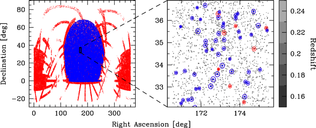
The total number of detected clusters in the whole photometric sample is $132683$, in the redshift range $0.05<z<0.8$. The detection rate increases with the cluster mass. Using X-ray and weak-lensing measurements available for a subsample of clusters, WHL12 showed that the sample is complete for $M_{200}\gtrsim 2\cdot 10^{14}M_{\odot}$ in the redshift range $0.1<z<0.42$, while the detection rate decreases down to $\sim 75\%$ for the minimum mass of the sample, $M_{200}=6\cdot 10^{13}M_{\odot}$ (see WHL12 for more details on the detection algorithm adopted). For this work, we use a subsample of clusters extracted from the WHL12 spectroscopic sample. Specifically, we consider the complete spectroscopic cluster sample from the Northern Galactic Cap, with measured redshifts in the range $0.1<z<0.42$. Moreover, we use only the SDSS stripes with at least $50\%$ of the clusters with spectroscopic redshift assigned. This is to obtain the largest contiguous area and to minimize possible selection effects. The final number of objects in our selected sample is $25226$. The left panel of Fig. 1 shows the angular distribution of the spectroscopic cluster sample (blue dots) analysed in this work, compared to the entire photometric sample (red dots), while the right panel shows a zoomed $5\times 5$ square degrees region, where grey dots represent galaxies from the SDSS DR8 photometric survey, and blue and red circles represent the angular projection of the cluster radii $r_{200}$, from the spectroscopic (blue) and photometric (red) samples, estimated using our fiducial cosmology.

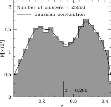
The main properties of the spectroscopic sample used for this work are summarized in Table 1. The photometric sample is used to compute the sampling rate, as described in §3.3. In Fig. 2 we show the redshift distribution of the selected spectroscopic clusters. The bimodal shape is due to the presence of two main spectroscopic targets in SDSS-II: the main sample that peaks around $z\sim 0.12$ (Strauss et al., 2002), and the LRG sample that covers the redshift range $0.2<z<0.5$ (Eisenstein et al., 2001).

3 Analysis

3.1 Two-point correlation function in real-space and redshift-space

We estimate the redshift-space two-point correlation function, $\xi(s)$, using the Landy & Szalay (1993) estimator:

$$\xi(s)\,=\,\frac{1}{RR(s)}\times\left[DD(s)\frac{n_{r}^{2}}{n_{d}^{2}}-2DR(s)\frac{n_{r}}{n_{d}}+RR(s)\right]\,,$$ (1)

where $DD(s)$, $DR(s)$ and $RR(s)$ are the numbers of weighted data-data, data-random and random-random pairs within a separation $s\pm\Delta s/2$, where $\Delta s$ is the bin size, and $n_{r}$ and $n_{d}$ are the weighted number density of random and cluster sample, respectively. To compute comoving distances and bias (see §3.5), we assume a flat $\Lambda$ cold dark matter (CDM) model with the mass density parameter $\Omega_{M}=0.3$, the baryon density parameter $\Omega_{b}=0.045$, the Hubble constant $H_{0}=70\,\mathrm{km}\,\mathrm{s}^{-1}\,\mathrm{Mpc}^{-1}$, the primordial perturbation spectral index $n_{s}=1$, and the linear power spectrum amplitude $\sigma_{8}=0.8$.

To derive the real-space clustering, we measure the projected correlation function:

$$w_{p}(r_{p})\,=\,\int_{0}^{\pi_{max}}\mathrm{d}\pi^{\prime}\xi(r_{p},\pi^{\prime})\,,$$ (2)

where $\xi(r_{p},\pi)$ is the measured two-point correlation function in the directions perpendicular, $r_{p}$, and parallel, $\pi$, to the line-of-sight. The real-space two-point correlation function, $\xi(r)$, is then obtained from $w_{p}$ assuming a power-law model, $\xi(r)=(r/R_{0})^{-\gamma}$, where $R_{0}$ and $\gamma$ are the correlation length and the power-law index, respectively. With the above assumption, the relation between $\xi$ and $w_{p}$ can be derived analytically:

$$w_{p}(r_{p})\,=\,r_{p}\left(\frac{R_{0}}{r_{p}}\right)^{\gamma}\frac{\Gamma(\frac{1}{2})\Gamma(\frac{\gamma-1}{2})}{\Gamma(\frac{\gamma}{2})}\,,$$ (3)

where $\Gamma$ is the Euler’s gamma function.

Figure 2: The redshift distribution of the selected galaxy clusters (histogram). The solid line shows the smoothed redshift distribution obtained adopting a Gaussian filter. See WHL12 for further details on the redshift distribution of the galaxy samples used to detect the clusters.

Table 1: Main properties of the spectroscopic cluster sample used for this work. See §2 for more details.

$\#$ objects	$25226$
Area $[\mathrm{deg}^{2}]$	$\sim 8400$
$z$ range	$0.1<z<0.42$
$\tilde{z}$	$0.268$
$R_{L^{*}}^{min}$	$12$
$M_{min}$	$6\cdot 10^{13}M_{\odot}$

3.2 Random sample

To measure the two-point correlation function of our sources, we have to construct a sample of randomly distributed objects (see Eq. 1), taking into account the selection function of the sample. As a fair approximation, we can factorise the random sample distributions into the angular and redshift components separately.

The angular mask is reconstructed with the software MANGLE (Swanson et al., 2008). Using the SDSS coordinates system $(\lambda,\eta)$, we decompose the angular distribution of clusters in rectangular elements of equal area, that are then randomly filled. We do not apply any weights to take into account sector completeness when creating the random sample.

We assign redshifts to the random objects sampling the mean redshift distribution of the catalogue. The latter has been obtained grouping the data in $100$ redshift bins and smoothing the distribution with a Gaussian kernel three times larger than the bin size. Reducing the value of this parameter has the effect to lower the clustering signal in the radial direction. The impact of this effect is however negligible, considering the estimated uncertainties in our measurements. To minimize the effect of shot noise, we construct a random sample ten times denser than the cluster sample. Fig. 2 shows the redshift distribution of the cluster sample (histogram) and the smoothed distribution (solid line) used for the construction of the random sample.

3.3 Weights

In this analysis, we apply three different weights to correct for i) the effects of a mass-dependent detection rate in the cluster selection algorithm, ${W}_{M_{200}}$ (see WHL12), and for ii) the spectroscopic sampling rate, as a function of the cluster richness, ${W}_{N_{200}}$, and of the stripe location, ${W_{S}}$, separately. We derive the above quantities directly from the data, comparing the photometric and spectroscopic cluster samples. For each cluster, the total weight assigned is:

$$w_{i}(R_{L^{*}},N_{200},stripe)={W}_{M_{200}}^{-1}\cdot{W}_{N_{200}}^{-1}\cdot{W}_{S}^{-1}\,.$$ (4)

The net effect is to increase the number of low mass structures, whose sampling rate is lower with respect to the more massive structures, in the spectroscopic sample. This slightly reduces the clustering normalization, up to $\sim 10\%$. On the contrary, we find that the BAO peak position is not affected by the details of the weighting scheme adopted.

3.4 Error estimates

The errors on the clustering measurements are estimated with the jackknife method (see e.g. Norberg et al., 2009). The covariance matrix for the jackknife estimator is:

$$C_{ij}\,=\,\frac{N_{sub}-1}{N_{sub}}\sum_{k=1}^{N}(\xi_{i}^{k}-\bar{\xi}_{i})(\xi_{j}^{k}-\bar{\xi}_{j})\,,$$ (5)

where $\xi_{i}^{k}$ is the value of the correlation function at the i-th bin for the k-th subsample, and $\bar{\xi}_{i}$ is the mean value of the subsamples.

We construct $N_{sub}=140$ resamplings of our cluster catalogue by dividing the original sample in $N_{sub}$ regions (i.e. $5$ subvolumes for each of the $28$ SDSS stripes considered) and excluding recursively one of them. Increasing the number of subregions provides a less scattered estimate of the covariance matrix. As verified directly, the value of $N_{sub}$ adopted here is large enough to assure the convergence of the results. We extensively test the jackknife algorithm exploited in this work using the LasDamas mock catalogues (McBride et al., 2009), finding that the quoted errors are conservative estimates.

3.5 Models

In the following sections, we describe the models used to derive clustering parameters and cosmological constraints from the projected correlation function and the BAO peak. The analysis is performed applying a Monte Carlo Markov Chain (MCMC) technique, using the full covariance matrix. We adopt a standard likelihood, $\mathscr{L}\propto\exp(-\chi^{2}/2)$, where the function $\chi^{2}$ is defined as follows:

$$\chi^{2}=\sum_{i=0}^{i=n}\sum_{j=0}^{j=n}(\xi_{i}-\hat{\xi}_{i})C^{-1}_{ij}(\xi_{j}-\hat{\xi}_{j})\,,$$ (6)

where $\xi_{i}$ is the correlation function measured in the i-th bin, $\hat{\xi}_{i}$ is the model and $C^{-1}_{ij}$ is the inverted covariance matrix.

3.5.1 The cluster bias

To measure the bias factor, $b$, we model the projected correlation function assuming a linear biasing model,

$$w_{p}(r_{p})=b^{2}w_{p}^{DM}(r_{p})\,,$$ (7)

where $w_{p}^{DM}$ is the DM projected correlation function (e.g. Marulli et al., 2013). When assessing the bias through Eq. 7, the upper limit of the integration in Eq. 2, $\pi_{max}$, has to be fixed. The impact of this parameter choice is not significant, considering the estimated uncertainties. Nevertheless, a finite value of $\pi_{max}$ introduces unavoidable systematic errors, as the effect of redshift-space distortions (RSD) can not be entirely washed out by the integration. The net effect is a spurious scale-dependence in the estimated bias. To minimize the impact of such a systematics, instead of using Eq.7 we model directly the projected correlation function as follows:

$$w_{p}(r_{p})\,=\,b^{2}\int_{0}^{\pi_{max}}\mathrm{d}\pi^{\prime}\xi^{\rm DM}(r_{p},\pi^{\prime})\,,$$ (8)

where the value of $\pi_{max}$ is the same as the one used to measure $w_{p}(r_{p})$ and $\xi^{\rm DM}(r_{p},\pi)$ is the redshift-space DM correlation function in the directions perpendicular and parallel to the line of sight. RSD are introduced with the dispersion model (Kaiser, 1987; Hamilton, 1992; Davis & Peebles, 1983), following Marulli et al. (2012). The linear DM correlation function is obtained by Fourier transforming the matter power spectrum computed with the software CAMB (Lewis & Bridle, 2002). The linear RSD parameter is estimated assuming a $\Lambda{\mathrm{CDM}}$ cosmology, i.e. $\beta=\Omega_{M}(z)^{\gamma}/b$, with $\gamma=0.545$.

As extensively tested, this method is able to compensate for the effect of RSD when integrating up to a finite value of $\pi_{max}$, providing an approximately scale-independent bias in the range of scales considered.

3.5.2 Cosmological constraints from the BAO peak

In this section, we descibe two different methods to detect the BAO peak and extract cosmological information. Results obtained with both the methods are presented in §4.2.

Empirical model

We consider an empirical model similar to the one proposed by Sánchez et al. (2012), which is used to interpolate the function $\xi(s)$ at the BAO scales:

$$\xi(s)\,=\,B+\left(\frac{s}{s_{0}}\right)^{-\gamma}+\frac{N}{\sqrt{2\pi\sigma^{2}}}\exp\left(-\frac{(s-s_{m})^{2}}{2\sigma^{2}}\right)\,,$$ (9)

where the parameters $s_{0}$ and $\gamma$ model the shape of the correlation at small scales, $B$ takes into account a possible negative correlation at large scales, and $s_{m}$, $\sigma$, and $N$ are the parameters of the Gaussian function used to model the BAO feature. We note that the true BAO peak position, $s_{p}$, is shifted to smaller scales with respect to the Gaussian median value $s_{m}$.

The empirical model given by Eq. 9 can be used to accurately detect the BAO peak position. To directly compare our measurements with previous studies, we compute also the dimensionless variable:

$$y_{s}=\frac{r_{s}}{D_{V}}\,,$$ (10)

that results to be independent of the fiducial cosmology assumed to derive comoving coordinates (see e.g. Sánchez et al., 2012). The distance $D_{V}$ is defined as:

$$D_{V}=\left[(1+z)^{2}D_{A}(z)^{2}\frac{cz}{H(z)}\right]^{\frac{1}{3}}\,,$$ (11)

where $D_{A}$ is the angular diameter distance and $H(z)$ is the Hubble function.

Physical model

To extract the full cosmological information embedded in the position of the BAO peak, we consider a theoretical model that includes the cluster bias, the effects of RSD and geometric distortions due to a possible incorrect assumption of the fiducial cosmology. The adopted model is the following:

$$\xi_{cl}(s)\,=\,b^{2}\,\left(1+\frac{2}{3}\beta+\frac{1}{5}\beta^{2}\right)\xi_{DM}(\alpha s)\,,$$ (12)

where $b$ is the linear bias factor, $\alpha$ is the ratio between the test and fiducial values of $D_{V}$ and it is used to model geometric distortions, and $\beta$ is the linear distortion parameter described in §3.5.1. The non-linear DM correlation function, $\xi_{DM}$, is computed using the software MPTbreeze (Crocce & Scoccimarro, 2008), based on the renormalized perturbation theory (Crocce & Scoccimarro, 2006). This method has already been used in previous works aimed at extracting cosmological information from the position of the BAO peak (see e.g. Eisenstein et al., 2005; Beutler et al., 2011; Blake et al., 2011).

To compare with previous studies, we exploit this method to derive also other parameters such as $y_{s}$ (see also §3.5), and the acoustic parameter $A(z)$, defined as follows:

$$A(z)\equiv\frac{100D_{V}(z)\sqrt{\Omega_{M}h^{2}}}{cz}\,.$$ (13)

This parameter results to be independent of $H_{0}$, since $D_{V}\propto H_{0}^{-1}$ (see e.g. Eisenstein et al., 2005; Blake et al., 2011).

Figure 3: The projected correlation function of galaxy clusters (black dots). The dashed grey line shows the best-fit linear model defined by Eq. 3, while the other three lines are the best-fit models obtained through Eq. 8 for three different values of the mass density parameter, $\Omega_{M}=0.25,0.3,0.35$.

4 Results

In this section, we present the main results of our analysis. We start focusing on the small scale clustering, estimating the linear bias from the projected correlation function at $r_{p}<30\,\mathrm{Mpc}\,h^{-1}\,$. Then, we move to larger scales, detecting the BAO peak and extracting cosmological information. Finally, we compare our measurements with previous studies.

Figure 4: Left panel: the redshift-space two-point correlation function of galaxy clusters (black dots), multiplied by $s^{2}$ to magnify the BAO peak; error bars are the square root of the diagonal elements of the covariance matrix, multiplied by $s^{2}$. The dashed green line is the best-fit empirical model obtained through Eq. 9. The blue line is the best-fit physical model given by Eq. 12, while the dot-dashed red line shows the no-BAO prediction, obtained with the fitting formula by Eisenstein & Hu (1999). Right panel: $\Delta\chi^{2}$ as a function of $D_{V}$, for the physical (blue line) and the no-BAO (red line) models. The BAO peak is detected with a $\sim 2.5\sigma$ confidence level.

4.1 Projected correlation function and bias

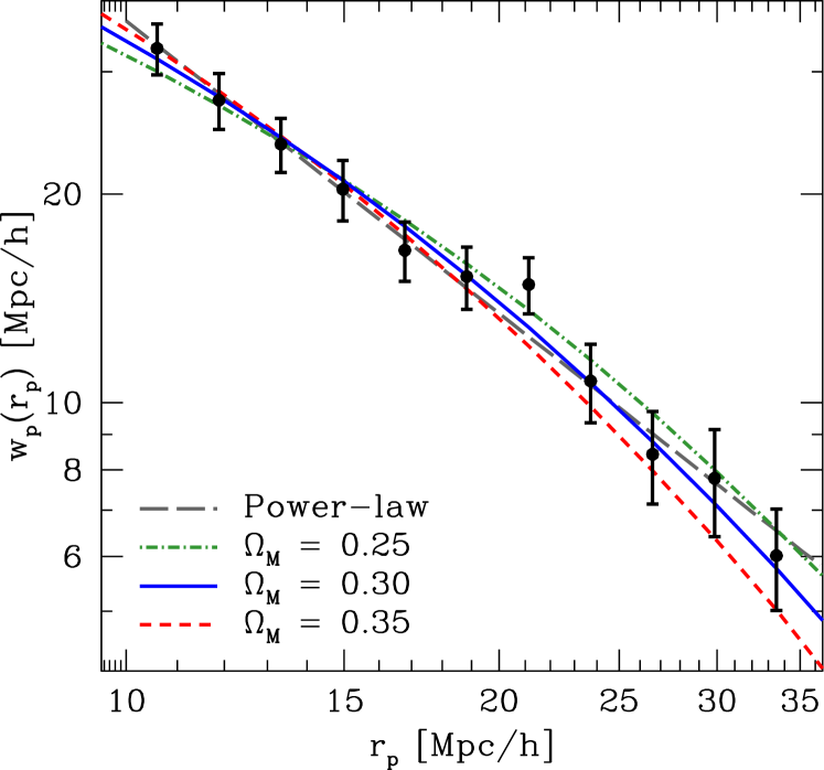
Fig. 3 shows the projected correlation function, $w_{p}(r_{p})$, estimated through Eq. 2. The error bars are the square root of the diagonal elements of the covariance matrix given by Eq. 5, i.e. $\sigma_{i}\,=\,\sqrt{C_{ii}}$. We derive the correlation length, $R_{0}$, and the power-law index, $\gamma$, assuming a power-law model for the real-space clustering, thus fitting the projected correlation function using Eq. 3. The result of the fit, obtained in the range of scales $10<r_{p}[\mathrm{Mpc}\,h^{-1}]<30$, is shown by the dashed grey line.

In Eq. 2 we set the upper limit of the integration to the value $\pi_{max}=40\,\mathrm{Mpc}\,h^{-1}$. We investigated the impact of this assumption and of the scale range used for the fit, repeating the procedure for different values of $\pi_{max}$ and of the scale limits. We find that our results are only marginally affected by these parameters. The maximum variation in $R_{0}$ and $\gamma$ is of the order of $7\%$, when $\pi_{max}$ and the scale limits are changed inside reasonable ranges (i.e. $20<\pi_{max}[\,\mathrm{Mpc}\,h^{-1}\,]<60$, $5<r_{p}[\,\mathrm{Mpc}\,h^{-1}\,]<60$).

We estimate the linear bias parameter, $b$, using the method described in §3.5.1. The DM correlation function is computed assuming the same fiducial cosmology used to measure comoving distances. The best-fit value of the bias, with 1$\sigma$ uncertainties, is $b\,\sigma_{8}=1.72\pm 0.03$, corresponding to a minimum $\chi^{2}$ value of $6.7$, with $10$ degrees of freedom. The best-fit values of $R_{0}$, $\gamma$ and $b\,\sigma_{8}$ are reported in Table 2.

To investigate the impact of the mass density parameter, we repeat the same measurement for $\Omega_{M}=0.25$ and $\Omega_{M}=0.35$. The three best-fit models corresponding to the three assumed values of $\Omega_{M}$ are shown in Fig. 3 with different lines, as indicated by the labels. The measured $w_{p}(r_{p})$ results to be only marginally affected by geometric distortions when changing $\Omega_{M}$, while this is not the case for the model. Therefore, the best-fit value of the bias does depend on $\Omega_{M}$ (e.g. Marulli et al., 2012). The best-fit values we obtain are the following: $b\,\sigma_{8}(\Omega_{M}=0.25)=1.55\pm 0.03$ and $b\,\sigma_{8}(\Omega_{M}=0.35)=1.88\pm 0.04$. In particular, we find that the best-fit bias values derived for different $\Omega_{M}$ are the ones that keep the value of $\beta$ approximately constant. The correspondent $\chi^{2}$ are: $\chi^{2}(\Omega_{M}=0.25)=8.6$ and $\chi^{2}(\Omega_{M}=0.35)=9.9$, respectively. The minimum of $\chi^{2}$ is obtained for $\Omega_{M}=0.3$, thus favouring the fiducial cosmology assumed in this work. In the next section we will perform a more detailed analysis, modelling the large scale clustering and constraining directly $\Omega_{M}$, with a full MCMC method, finding consistent results.

We notice that our analysis shows a lower clustering with respect to the estimates by Estrada et al. (2009) and Hong et al. (2012). This is due to the lower mass limit in our cluster sample, that results in a lower bias.

4.2 The BAO peak

4.2.1 Fitting with the empirical model

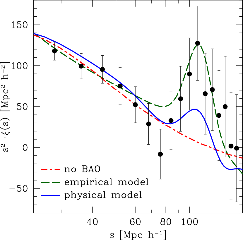
The left panel of Fig. 4 shows the redshift-space two-point correlation function, $\xi(s)$, multiplied by $s^{2}$, in order to magnify the BAO peak. We start fitting the clustering data with the empirical model given by Eq. 9, in the scale range $20<s[\,\mathrm{Mpc}\,h^{-1}\,]<180$, using a MCMC technique. The result of the fit is shown by the dashed green line. The best-fit value of the peak position is $s_{p}=104\pm_{6}^{7}\,\mathrm{Mpc}\,h^{-1}\,$, after marginalizing over the other $5$ parameters of the model. When using linear instead of logarithmic binning, the BAO peak results slightly shifted to higher values. However, the effect is of the order of $2\%$, well below the estimated accuracy on the BAO peak position, that is of the order of $7\%$. We also fit the data with the same empirical model but without the Gaussian part. The $\Delta\chi^{2}$ gives a confidence level for the full model between $2$ and $3\sigma$.

Our measurement is in good agreement with the previous detection by Hong et al. (2012). Moreover, thanks to the higher cluster density in our sample, that is larger by a factor of two, the uncertainty in the position of the BAO peak is significantly lower.

4.2.2 Fitting with the physical model

We now fit the measured correlation function with the physical model described in §3.5. Cosmological information is encoded in $\Omega_{M}h^{2}$, in the linear bias $b$, and in the shift parameter, $\alpha$, that traces geometrical distortions. All the other cosmological parameters are kept fixed to the Planck values: $H_{0}=67.4\,\mathrm{km\,s^{-1}\,Mpc^{-1}}$, $\Omega_{b}=0.02207h^{2}$, $n_{s}=0.96$ and $\sigma_{8}=0.83$ (Planck Collaboration, 2013).

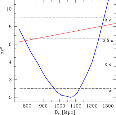
The best-fit parameters are summarized in Table 2. The reported values are the medians of the MCMC parameter distributions, while the $1\sigma$ errors span from the $16th$ to the $86th$ percentiles. The solid blue line in the left panel of Fig. 4 shows the result of the fit obtained using the MPTbreeze software to estimate $\xi_{DM}(r)$, while the red one has been obtained using the fitting formula given by Eisenstein & Hu (1999) with no BAO. As shown in the right panel of Fig. 4, the BAO feature is detected with a $\sim 2.5\sigma$ confidence level, in agreement with what obtained with the empirical model. We achieve a distance measure of $D_{V}=1031\pm_{92}^{84}$. Constraints on the distortion parameters $y_{s}$ are of the order of $7\%$, in good agreement with the value obtained with the empirical model in §3.5. Fitting in the range $20<s[\,\mathrm{Mpc}\,h^{-1}\,]<180$, we obtain a $10\%$ constraint on the mass density parameter, $\Omega_{M}h^{2}=0.15\pm_{0.02}^{0.03}$, after marginalizing over the other two model parameters $\alpha$ and $b$ (see §3.5). Reducing the fitting range has the effect of slightly worsening the constraints.

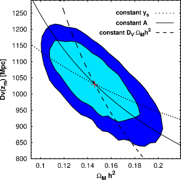
Fig. 5 shows the $1$ and $2\sigma$ marginalized probability contours in the $\Omega_{M}h^{2}-D_{V}$ plane. The dotted line indicates the points with constant $y_{s}$, i.e. it represents the degeneracy direction between parameters that would occur if the fit was driven by the BAO feature only. The dashed line shows the opposite case in which the fit is driven only by the shape of the two-point correlation function. As it can be seen, the orientation of the parameter degeneracy obtained in this work lies approximately in the middle between these two extremes, closely following the solid line of costant $A$ (Eq. 13). In Table 2 we report the best-fit values of the cosmological parameters, as well as the estimated uncertainties derived from the MCMC analysis after marginalizing over all the free parameters of the fit. As it can be seen, the estimated value of $b$ is consistent with the one derived in §4.1 by fitting the projected correlation function at smaller scales.

Figure 5: Marginalized probability contours at $1$ and $2\sigma$ for $\Omega_{M}h^{2}-D_{V}$, obtained fitting Eq. 12 in the scale range $20<s[\,\mathrm{Mpc}\,h^{-1}\,]<180$. The red cross marks the median values of the two parameters from the MCMC realizations. The dotted line is obtained keeping fixed $y_{s}$ at the best-fit value, indicating a pure BAO-scale driven fit. The continuous line shows the same but for the parameter $A$ (Eq. 13). The dashed line is obtained keeping fixed the value of $D_{V}\Omega_{M}h^{2}$.

Table 2: Best-fit parameters and 1 $\sigma$ uncertainties obtained from the projected and redshift-space two-point correlation functions of the selected spectroscopic cluster sample. For more details see §3.5.1 and §3.5.2.

Statistics	Parameters	Best-fit values, $1\sigma$ uncertainties
	$R_{0}$ $[\,\mathrm{Mpc}\,h^{-1}\,]$	$11.4\pm 0.4$
$w_{p}(r_{p})$	$\gamma$	$2.3\pm 0.1$
	$b\,\sigma_{8}$	$1.72\pm 0.03$
	$s_{p}$ $[\,\mathrm{Mpc}\,h^{-1}\,]$	$104\pm_{6}^{7}$
	$D_{V}(\tilde{z})$ $[\mathrm{Mpc}]$	$1031\pm_{92}^{84}$
$\xi(s)$	$y_{s}$	$0.147\pm_{0.008}^{0.010}$
	$A(\tilde{z})$	$0.48\pm_{0.03}^{0.03}$
	$\Omega_{M}\,h^{2}$	$0.15\pm_{0.02}^{0.03}$
	$b\,\sigma_{8}$	$1.6\pm_{0.2}^{0.1}$

4.3 Comparison with previous BAO measurements

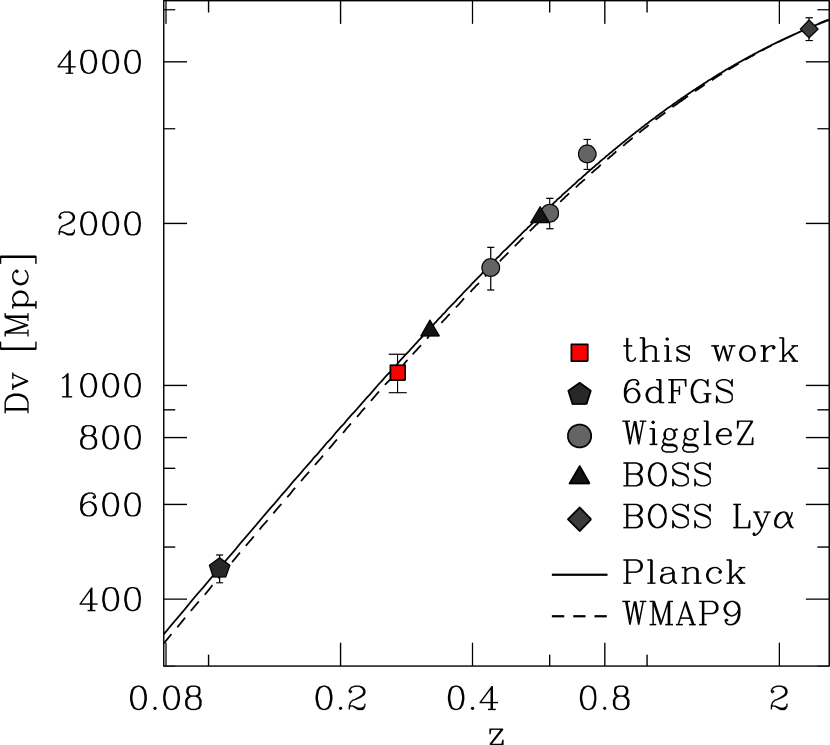
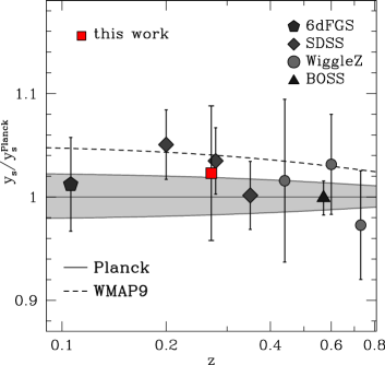
To compare our measurements with similar results in the literature, we estimate the dimensionless variable $y_{s}=s_{p}/D_{V}$ as described in §3.5, assuming the median redshift of the sample, $\tilde{z}=0.268$, as the reference redshift. In our fiducial cosmological framework, we have $y_{s}=0.147\pm_{0.008}^{0.010}$, as reported also in Table 2.

In Fig. 6 we compare our measurements (red squares) of $D_{V}$ (left panel) and $y_{s}$ (right panel) with previous estimates from large galaxy surveys at different redshifts. The $y_{s}$ values are normalized to the $\Lambda\mathrm{CDM}$ prediction, $y_{s}^{\rm ref}(z)$, evaluated through CAMB using the Planck cosmological parameters (Planck Collaboration, 2013). The shaded area is obtained changing the mass density parameter in the range ${\Omega_{M}-0.04,\Omega_{M}+0.04}$, where the central value is set to the Planck value $\Omega_{M}h^{2}=0.1423$. All the measurements appear compatible with the $\Lambda{\mathrm{CDM}}$ predictions for both WMAP9 and Planck parameters. As it can be seen, the uncertainties estimated in this work are competitive with what found with large galaxy surveys, despite the sparseness of the spectroscopic cluster sample considered. However, due to the present uncertainties, we are not yet able to distinguish between the two sets of cosmological parameters given by WMAP9 and Planck.

Figure 6: $D_{V}$ (left panel) and $y_{s}$ (right panel) as a function of redshift. Comparison of our measurements (red square) with previous estimates from large galaxy samples (grey/black symbols): 6dF Galaxy Survey ($z=0.106$ by Beutler et al. 2011), SDSS ($z=0.2,0.35$ by Percival et al. 2010; $z=0.278$ by Kazin et al. 2010), WiggleZ ($z=0.44,0.6$ and $0.73$ by Blake et al. 2011) and BOSS ($z=0.35,z=0.57$ by Anderson et al. 2012) and BOSS $Ly\alpha$ ($z=2.34$ by Delubac et al. 2014). Solid and dashed lines show the $\Lambda{\mathrm{CDM}}$ predictions obtained adopting the Planck and WMAP9 parameters, respectively. The $y_{s}(z)$ values are normalized to the Planck values. The shaded area is obtained changing the mass density parameter in the range $\{\Omega_{M}-0.04,\Omega_{M}+0.04\}$, where the central value is set to the Planck value $\Omega_{M}h^{2}=0.1423$.

5 Discussion

The cluster centres of the spectroscopic sample analysed in this work are determined by the positions of the BCGs (see §2). Therefore, the cluster clustering presented in previous sections corresponds exactly to the clustering of the BCG sample, that is about a subsample of LRGs. The latter has obviously a larger level of shot-noise compared to a full LRG sample. Thus, it is worth wondering if there is any advantage of using a sparse cluster sample, instead of a larger galaxy sample, for BAO analyses. We address this question in §5.1, where we compare directly the two-point correlation function measured in a large LRG sample to the one of a subsample of BCGs. Finally, in §5.2 we compare the clustering of our spectroscopic cluster sample with a larger photometric sample, investigating the impact of photometric redshift errors.

5.1 Clusters vs LRGs

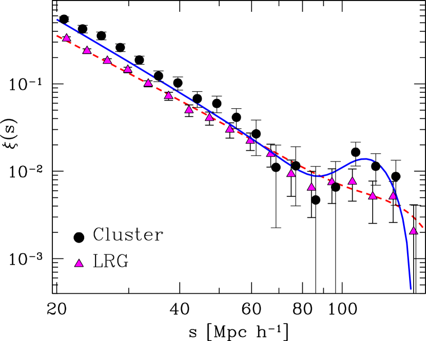
For any clustering analysis, the WHL12 spectroscopic cluster sample can be considered just as a particularly selected subsample of LRGs. To investigate the impact of such a selection on the detection of the BAO peak, we consider here the large LRG sample by Kazin et al. (2010). The catalogue consists of $\sim 66000$ galaxies extracted from the SDSS Data Release 7, in the redshift range $0.16<z<0.36$. To avoid any possible systematic effect, we restrict our analysis to the Northern Galactic Cap, reducing the number of objects to $\sim 59000$, with a median redshift of $\tilde{z}=0.278$. Then, we identify the BCGs included in the LRG sample, thus obtaining the analogous of a spectroscopic cluster catalogue. This BCG catalogue contains $\sim 15000$ objects, with a median absolute magnitude larger that that of the LRG sample. The redshift-space two-point correlation functions of the LRG (magenta triangles) and BCG (black dots) samples are compared in the left panel of Fig. 7. The two populations show a different linear bias, $b_{BCG}/b_{LRG}\sim 1.16$. Moreover, while the $1\sigma$ error bars are smaller for the LRGs, due to their higher number density, the BAO peak is significantly better determined for the BCG sample. Following the same analysis performed in §3.5.2, we find that the significance of the BAO detection in the LRG sample is at less than $1.5\sigma$ level, and the error on the BAO peak results more than two times larger relative to the one obtained with the BCG sample. To investigate the robustness of our data reduction and clustering measurements, we compare our results with the literature (Kazin et al., 2010), finding good agreement and confirming that our jackknife method slightly overpredicts the uncertainties relative to external methods based on mock catalogues, thus providing conservative estimates for the errors.

To further investigate the differences between BCG and LRG clustering, we extract two subsamples of LRGs with the same number of objects, one totally random and the other reproducing the BCG absolute magnitude distribution. Then we measure the two-point correlation function for both the samples, and we repeat the BAO analysis. In both cases, we find that the BAO peak is less accurately determined with respect to the BCG case. We conclude that BCGs, or equivalently galaxy clusters, are optimal tracers to detect the BAO peak. This is due to the dynamical state of these objects, that have significantly lower peculiar velocities with respect to other galaxies. Indeed, as we verified directly, the Fingers of God feature is almost absent in the BCG sample analysed here. This is the crucial property that can reduce the width of the BAO peak, thus improving the significance of the detection. Actually, such a small scale effect can directly impact the large scale clustering, as clearly shown in Fig. 7.

Figure 7: Comparison between the redshift-space two-point correlation functions of cluster (black dots) and LRG (magenta triangles) spectroscopic samples (left panel), and between spectroscopic (black dots) and photometric (magenta triangles) cluster samples (right panel). The lines show the best-fit empirical models obtained through Eq. 9, for spectroscopic clusters (blue lines) and photometric clusters/LRG (dashed red lines).

5.2 Spectroscopic sample vs photometric sample

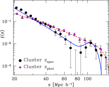
The effect of small scale dynamics on the two-point correlation function appears quite similar to the one of redshift errors (Marulli et al., 2012). Thus, for what we have seen in §5.1, we expect that photometric redshift errors can have a significant impact also at the BAO scales. To investigate this effect, we consider the large photometric cluster sample provided by WHL12, that contains more than $120000$ objects identified using a Friends-of-Friends algorithm. The redshift of the identified galaxy clusters is the mean of the photometric redshifts of their components. The cluster photometric redshifts result highly scattered around the spectroscopic redshifts, with a standard deviation of $\sim 0.015$, as estimated in Wen et al. (2012).

The right panel of Fig. 7 shows the comparison between the redshift-space two-point correlation function of photometric (magenta triangles) and spectroscopic (black dots) cluster samples, in the redshift range $0.1<z<0.42$. The number of photometric clusters is almost twice bigger than the spectroscopic one. However, as it can be seen, the large photometric redshift errors reduce the clustering slope (Marulli et al., 2012) and, most importantly, they broaden the BAO feature, causing a loss of information at the BAO scale. Indeed, the larger number of clusters does not compensate for the poor redshift measurements.

Finally, to further test this effect, we add Gaussian redshift errors to the spectroscopic sample, repeating the analysis for different values of the error. We find that the determination of the BAO peak is quite robust for redshift errors lower than $0.005$, and then it rapidly degrades.

6 Conclusions

In this paper we presented new measurements of the two-point correlation function of a spectroscopic sample of galaxy clusters, selected from the SDSS (WHL12) in the redshift range $0.1<z<0.42$. From the projected correlation function, we derive the correlation length and the power-law index of the real-space clustering, and the linear bias factor. As shown in Fig. 4, we could clearly detect the BAO peak. Fitting the measured $\xi(s)$ with an empirical model with a Gaussian function at the BAO scale, we find $s_{p}=104\pm_{6}^{7}\,\mathrm{Mpc}\,h^{-1}\,$, $y_{s}=0.147\pm_{0.008}^{0.010}$ and $D_{V}=1031\pm_{92}^{84}\,\mathrm{Mpc}\,h^{-1}\,$. We test two different methods to analyse the BAO feature, both providing compatible constraints. We estimate a confidence level in the BAO detection of $\sim 2.5\sigma$, despite the sparseness of the spectroscopic cluster sample considered. This is comparable to what obtained from many large galaxy surveys, though the latest measurements provide even stronger constraints, e.g. SDSS DR11 LRGs and QSO Ly-$\alpha$ provide $\sim 7\sigma$ and $\sim 5\sigma$ BAO detection, respectively (Anderson et al., 2014; Delubac et al., 2014). Overall, our measurements appear consistent with all previous studies and with the $\Lambda\mathrm{CDM}$ predictions. Our error estimates are quite conservative, due to the method used to compute the covariance matrix. The goodness of our results is due to the high clustering signal (i.e. high bias) of the cluster sample analysed, and to the accuracy in the spectroscopic redshift measurements. Indeed, as we have verified directly, the BAO peak is weakly constrained when using larger LRG or photometric cluster catalogues. This result shows that galaxy clusters are powerful cosmological probes for the detection of BAO, even with a fairly limited statistics, and highly competitive with respect to galaxies. Future massive surveys such as Euclid (Laureijs et al., 2011; Amendola et al., 2013) and eROSITA (Merloni et al., 2012) will allow this approach to be fully exploited in several open key questions (e.g. the dark energy equation of state). Accurate forecasts on the cosmological constraints achievable by these future cluster surveys will be provided in a future work. Moreover, thanks to the ongoing BOSS program, we plan to enrich the spectroscopic cluster sample analysed in this work, providing new BAO constraints at different redshifts, and as a function of the cluster richness.

References

- Aihara et al. (2011) Aihara H., Allende Prieto C., An D., et al., 2011, ApJS, 193, 29
- Amendola et al. (2013) Amendola, L., Appleby, S., Bacon, D., et al. 2013, Living Reviews in Relativity, 16, 6
- Anderson et al. (2012) Anderson L., Aubourg E., Bailey S., et al., 2012, MNRAS, 427, 3435
- Anderson et al. (2014) Anderson, L., Aubourg, É., Bailey, S., et al. 2014, MNRAS, 441, 24
- Angulo et al. (2005) Angulo, R. E., Baugh, C. M., Frenk, C. S., et al. 2005, MNRAS, 362, L25
- Beutler et al. (2011) Beutler F., Blake C., Colless M., et al., 2011, MNRAS, 416, 3017
- Blake et al. (2011) Blake C., Kazin E. A., Beutler F., et al., 2011, MNRAS, 418, 1707
- Blanton et al. (2003) Blanton M. R., Hogg D. W., Bahcall N. A., et al., 2003, ApJ, 592, 819
- Cole et al. (2005) Cole S., et al., 2005, MNRAS, 362, 505
- Crocce & Scoccimarro (2006) Crocce M., & Scoccimarro R. 2006, PhRvD, 73, 063519
- Crocce & Scoccimarro (2008) Crocce M., Scoccimarro R., 2008, PhRvD, 77, 023533
- Davis & Peebles (1983) Davis, M., & Peebles, P. J. E. 1983, ApJ, 267, 465
- Delubac et al. (2014) Delubac, T., Bautista, J. E., Busca, N. G., et al. 2014, arXiv:1404.1801
- Eisenstein & Hu (1999) Eisenstein, D. J., & Hu, W. 1999, ApJ, 511, 5
- Eisenstein et al. (2001) Eisenstein, D. J., Annis, J., Gunn, J. E., et al. 2001, AJ, 122, 2267
- Eisenstein et al. (2005) Eisenstein D. J., et al., 2005, ApJ, 633, 560
- Estrada et al. (2009) Estrada J., Sefusatti E., Frieman J. A., 2009, ApJ, 692, 265
- Hamilton (1992) Hamilton, A. J. S. 1992, ApJL, 385, L5
- Hong et al. (2012) Hong T., Han J. L., Wen Z. L., et al., 2012, ApJ, 749, 81
- Hütsi (2010) Hütsi G., 2010, MNRAS, 401, 2477
- Kaiser (1987) Kaiser, N. 1987, MNRAS, 227, 1
- Kazin et al. (2010) Kazin E. A., Blanton M. R., Scoccimarro R., et al., 2010, ApJ, 710, 1444
- Koester et al. (2007) Koester, B. P., McKay, T. A., Annis, J., et al. 2007, ApJ, 660, 239
- Komatsu et al. (2011) Komatsu, E., Smith, K. M., Dunkley, J., et al. 2011, ApJS, 192, 18
- Landy & Szalay (1993) Landy S. D., Szalay A. S., 1993, ApJ, 412, 64
- Laureijs et al. (2011) Laureijs R., Amiaux J., Arduini S., et al., 2011, ArXiv e-prints
- Lewis & Bridle (2002) Lewis A., Bridle S., 2002, PhRvD, 66, 103511
- Marulli et al. (2012) Marulli, F., Bianchi, D., Branchini, E., et al. 2012, MNRAS, 426, 2566
- Marulli et al. (2013) Marulli, F., Bolzonella, M., Branchini, E., et al. 2013, A&A, 557, A17
- McBride et al. (2009) McBride, C., Berlind, A., Scoccimarro, R., et al. 2009, Bulletin of the American Astronomical Society, 41, #425.06
- Merloni et al. (2012) Merloni, A., Predehl, P., Becker, W., et al. 2012, arXiv:1209.3114
- Norberg et al. (2009) Norberg P., Baugh C. M., Gaztañaga E., Croton D. J., 2009, MNRAS, 396, 19
- Padmanabhan et al. (2012) Padmanabhan N., Xu X., Eisenstein D. J., et al., 2012, MNRAS, 427, 2132
- Percival et al. (2007) Percival W. J., Cole S., Eisenstein D. J., Nichol R. C., Peacock J. A., Pope A. C., Szalay A. S., 2007, MNRAS, 381, 1053
- Percival et al. (2010) Percival W. J., Reid B. A., Eisenstein D. J., et al., 2010, MNRAS, 401, 2148
- Planck Collaboration (2013) Planck Collaboration, 2013, arXiv:1303.5076
- Sánchez et al. (2009) Sánchez A. G., Crocce M., Cabré A., Baugh C. M., Gaztañaga E., 2009, MNRAS, 400, 1643
- Sánchez et al. (2012) Sánchez A. G., Scóccola C. G., Ross A. J., et al., 2012, MNRAS, 425, 415
- Sánchez et al. (2011) Sánchez E., Carnero A., García-Bellido J., et al., 2011, MNRAS, 411, 277
- Slosar et al. (2013) Slosar, A., Iršič, V., Kirkby, D., et al. 2013, J. Cosm. Astro-Particle Phys., 4, 26
- Smith et al. (2003) Smith R. E., Peacock J. A., Jenkins A., et al., 2003, MNRAS, 341, 1311
- Strauss et al. (2002) Strauss, M. A., Weinberg, D. H., Lupton, R. H., et al. 2002, AJ, 124, 1810
- Swanson et al. (2008) Swanson M. E. C., Tegmark M., Hamilton A. J. S., Hill J. C., 2008, MNRAS, 387, 1391
- Wen et al. (2009) Wen, Z. L., Han, J. L., & Liu, F. S. 2009, ApJS, 183, 197
- Wen et al. (2012) Wen Z. L., Han J. L., Liu F. S., 2012, ApJS, 199, 34