Corner Detection and Arc Approximation of Planar Data Set

Maurizio Scarparo

ย  {onecolabstract} The aim of this paper is to present a new method of approximation of planar data set using only arcs or segments. The first problem we are trying to solve is the following: the CNC machines can work only with simple curves (arcs or segments, indeed). So, if we have a contour of an object and we want to cut, for example, glass or metal following that profile, we need a continuous curve composed by linear or circular paths only. Moreover, we want to minimize the number of these paths. The second problem is the following: the contour of an object is detected by a specific laser, which collects a discrete data set. The laser detects a good approximation of a point if this point is not a corner of the object. So in many cases our data set will not contain the real corners. Our task is to present a method on how to find these particular points. A third purpose is to study the regularity of the approximating curve, which can be G1superscript๐บ1G^{1} or C0superscript๐ถ0C^{0} continuous. The entire method is developed using single arcs, segments and in certain cases biarcs, in order to ensure the smoothness of the final path.

Keywords: arcs, biarcs, least-square fitting, point approximation, corner detection, digital curves

Contacts: maurizio.scarparo24@gmail.com ย ย ย ย ย ย ย ย 

1 Introduction

The problem of approximation of planar data set has been already studied by several authors, such as Les A. Piegl, Wayne Tiller, Hyungjun Park, D. Meek, D. Walton (see page 17). In their articles these authors explain the biarc model and how to apply it in CNC machining. One of the most powerful methods, introduced by Piegl and Tiller, consists in finding the least square B-spline and approximating this one with biarcs (see [7], [8], [9]). The problem of corner detection has also been studied by authors such as C. Harris, M. Stephens, H. Freeman, L. Davis. However, we decided to analyze these problems in a different way. The first task was to elaborate a new method of approximating a planar data set without using B-splines. Indeed, we found out that the B-spline method is very powerful when the data set has no corner points, but it is quite difficult to get a good approximation when the data set is not smooth. Moreover, we found out that the approximation heavily depends on the data set and on the choice of the tangent vectors, so we wanted to cancel the dependence on the vectors. We also discovered that single arcs are better than biarcs if we want to minimize the number of paths. Secondly, we wanted to develop a straightforward method for corner detection in a planar data set captured by a laser. As already explained in the abstract, this data set may not include the exact corner points, because of the laser errors. This is the main difference between our algorithm and the methods explained in [1], [2], [6], [11], [12]: all methods developed there need the corner points to be included in the data set. We noticed that this problem has been carefully studied for digital images using pixel properties, but as far as we know there are not many articles concerning this topic outside image analysis.

2 Least square constrained arcs

The first time we try to approximate a planar data set with only biarcs we can find out an inconvenient: if the distance between two consecutive points is small and the tangent vectors are quite different, the biarc between the two points will be serpentine, that means useless and insignificant for a good approximation. So the first step is to forget the biarc model for a while and to focus on the least square constrained arcs. Let ๐0subscript๐0\mathbf{P}_{0} 111Notation: ๐i=[xi,yi]subscript๐๐‘–subscript๐‘ฅ๐‘–subscript๐‘ฆ๐‘–\mathbf{P}_{i}=[x_{i},y_{i}], ๐1subscript๐1\mathbf{P}_{1}, โ€ฆโ€ฆ\dots, ๐N+1subscript๐๐‘1\mathbf{P}_{N+1} be N+2๐‘2N+2 distinct planar points. We want to find one particular arc with initial point ๐0subscript๐0\mathbf{P}_{0}, final point ๐N+1subscript๐๐‘1\mathbf{P}_{N+1}, approximating ๐1subscript๐1\mathbf{P}_{1}, โ€ฆโ€ฆ\dots, ๐Nsubscript๐๐‘\mathbf{P}_{N} and minimizing an objective error function. Let R๐‘…R, ๐‚๐‚\mathbf{C}, be respectively the radius and the center of our arc. The function we want to minimize is the following:

fโ€‹(t)=โˆ‘k=1N|Rโˆ’โ€–๐kโˆ’๐‚โ€‹(t)โ€–|2.๐‘“๐‘กsuperscriptsubscript๐‘˜1๐‘superscript๐‘…normsubscript๐๐‘˜๐‚๐‘ก2f(t)=\sum_{k=1}^{N}{\bigg{|}R-\parallel\mathbf{P}_{k}-\mathbf{C}(t){\parallel}\bigg{|}}^{2}. (1)

The variable t๐‘กt represents the distance between the centre C๐ถC and the segment ๐0โ€‹๐N+1ยฏยฏsubscript๐0subscript๐๐‘1\overline{\mathbf{P}_{0}\mathbf{P}_{N+1}}. In particular, let d=โ€–๐N+1โˆ’๐0โ€–๐‘‘normsubscript๐๐‘1subscript๐0d=\ \parallel\mathbf{P}_{N+1}-\mathbf{P}_{0}\parallel be the distance between ๐0subscript๐0\mathbf{P}_{0} and ๐N+1subscript๐๐‘1\mathbf{P}_{N+1}, let ๐ฎ๐ฎ\mathbf{u} be the normalized vector

๐ฎ=๐N+1โˆ’๐0d๐ฎsubscript๐๐‘1subscript๐0๐‘‘\mathbf{u}=\frac{\mathbf{P}_{N+1}-\mathbf{P}_{0}}{d} (2)

and let ๐ฎโ€ฒsuperscript๐ฎโ€ฒ{\mathbf{u}}^{\prime} be the ฯ€2๐œ‹2\frac{\pi}{2} counterclockwise rotation of ๐ฎ๐ฎ\mathbf{u}. Then, the center ๐‚๐‚\mathbf{C} can be represented by the following:

๐‚โ€‹(t)=๐0+d2โ€‹๐ฎ+tโ€‹๐ฎโ€ฒ.๐‚๐‘กsubscript๐0๐‘‘2๐ฎ๐‘กsuperscript๐ฎโ€ฒ\mathbf{C}(t)=\mathbf{P}_{0}+\frac{d}{2}\mathbf{u}+t{\mathbf{u}}^{\prime}. (3)

Let us discuss about the objective function (1). This is a non negative continous function on โ„โ„\mathds{R}. One can think that f๐‘“f depends on two unknown R๐‘…R and ๐‚๐‚\mathbf{C}; however, since the initial point of our arc is ๐0subscript๐0\mathbf{P}_{0} and the final one is ๐N+1subscript๐๐‘1\mathbf{P}_{N+1}, the radius depends on the center and

Rโ€‹(t)=โ€–๐0โˆ’๐‚โ€‹(t)โ€–=โ€–๐N+1โˆ’๐‚โ€‹(t)โ€–.๐‘…๐‘กnormsubscript๐0๐‚๐‘กnormsubscript๐๐‘1๐‚๐‘กR(t)=\ \parallel\mathbf{P}_{0}-\mathbf{C}(t)\parallel\ =\ \parallel\mathbf{P}_{N+1}-\mathbf{C}(t)\parallel. (4)

So, according to (4), the function f๐‘“f in (1) becomes

fโ€‹(t)=Nโ€‹โ€–๐0โˆ’๐‚โ€‹(t)โ€–2+โˆ‘k=1Nโ€–๐kโˆ’๐‚โ€‹(t)โ€–2โˆ’2โ€‹โ€–๐0โˆ’๐‚โ€‹(t)โ€–โ€‹โˆ‘k=1Nโ€–๐kโˆ’๐‚โ€‹(t)โ€–.๐‘“๐‘ก๐‘superscriptdelimited-โˆฅโˆฅsubscript๐0๐‚๐‘ก2superscriptsubscript๐‘˜1๐‘superscriptdelimited-โˆฅโˆฅsubscript๐๐‘˜๐‚๐‘ก22delimited-โˆฅโˆฅsubscript๐0๐‚๐‘กsuperscriptsubscript๐‘˜1๐‘delimited-โˆฅโˆฅsubscript๐๐‘˜๐‚๐‘ก\begin{split}f(t)=\ &N{\parallel\mathbf{P}_{0}-\mathbf{C}(t)\parallel}^{2}+\sum_{k=1}^{N}{\parallel\mathbf{P}_{k}-\mathbf{C}(t)\parallel}^{2}\\ &-2\parallel\mathbf{P}_{0}-\mathbf{C}(t)\parallel\sum_{k=1}^{N}{\parallel\mathbf{P}_{k}-\mathbf{C}(t)\parallel}.\end{split} (5)

According to Weierstrass theorem, f๐‘“f admits minimum on each compact set [a,b]โŠ‚โ„๐‘Ž๐‘โ„[a,b]\subset\mathds{R}. Moreover, one can easily see that the first derivative of f๐‘“f is always continuous on โ„โ„\mathds{R} if the center ๐‚โ€‹(t)๐‚๐‘ก\mathbf{C}(t) and the points ๐ksubscript๐๐‘˜\mathbf{P}_{k} are distinct for every k=0,1,โ€ฆ,N+1๐‘˜01โ€ฆ๐‘1k=0,1,\dots,N+1. We will prove that f๐‘“f admits finite limits at ยฑโˆžplus-or-minus\pm\infty and these limits are the same.

Theorem 2.1.

f๐‘“f has finite limit at ยฑโˆžplus-or-minus\pm\infty and

limtโ†’ยฑโˆžfโ€‹(t)=โˆ‘i=1N[๐ฎโ€ฒโ‹…(๐0โˆ’๐i)]2,subscriptโ†’๐‘กplus-or-minus๐‘“๐‘กsuperscriptsubscript๐‘–1๐‘superscriptdelimited-[]โ‹…superscript๐ฎโ€ฒsubscript๐0subscript๐๐‘–2\lim_{t\to\pm\infty}f(t)=\sum_{i=1}^{N}{\bigg{[}\mathbf{u}^{\prime}\cdot{(\mathbf{P}_{0}-\mathbf{P}_{i})}\bigg{]}}^{2}, (6)

where โ‹…โ‹…\cdot means the standard scalar product in โ„2superscriptโ„2{\mathds{R}}^{2}.

Proof.

We have that

โ€–๐0โˆ’๐‚โ€‹(t)โ€–2=โ€–d2โ€‹๐ฎ+tโ€‹๐ฎโ€ฒโ€–2=t2+d24,โ€–๐iโˆ’๐‚โ€‹(t)โ€–2=t2+2โ€‹tโ€‹[๐ฎโ€ฒโ‹…(๐0โˆ’๐i+d2โ€‹u)]+โ€–๐0โˆ’๐i+d2โ€‹uโ€–2.formulae-sequencesuperscriptdelimited-โˆฅโˆฅsubscript๐0๐‚๐‘ก2superscriptdelimited-โˆฅโˆฅ๐‘‘2๐ฎ๐‘กsuperscript๐ฎโ€ฒ2superscript๐‘ก2superscript๐‘‘24superscriptdelimited-โˆฅโˆฅsubscript๐๐‘–๐‚๐‘ก2superscript๐‘ก22๐‘กdelimited-[]โ‹…superscript๐ฎโ€ฒsubscript๐0subscript๐๐‘–๐‘‘2usuperscriptdelimited-โˆฅโˆฅsubscript๐0subscript๐๐‘–๐‘‘2u2\begin{split}&{\parallel\mathbf{P}_{0}-\mathbf{C}(t)\parallel}^{2}={\bigg{\|}\frac{d}{2}\mathbf{u}+t\mathbf{u}^{\prime}\bigg{\|}}^{2}=t^{2}+\frac{d^{2}}{4},\\ &{\parallel\mathbf{P}_{i}-\mathbf{C}(t)\parallel}^{2}=t^{2}+2t\bigg{[}\mathbf{u}^{\prime}\cdot\bigg{(}\mathbf{P}_{0}-\mathbf{P}_{i}+\frac{d}{2}\textbf{u}\bigg{)}\bigg{]}\\ &+{\bigg{\|}\mathbf{P}_{0}-\mathbf{P}_{i}+\frac{d}{2}\textbf{u}\bigg{\|}}^{2}.\end{split} (7)

Let ๐ƒi=๐0โˆ’๐i+d2โ€‹usubscript๐ƒ๐‘–subscript๐0subscript๐๐‘–๐‘‘2u\mathbf{D}_{i}=\mathbf{P}_{0}-\mathbf{P}_{i}+\frac{d}{2}\textbf{u}. We notice that f๐‘“f is the sum of N๐‘N functions fiโ€‹(t)subscript๐‘“๐‘–๐‘กf_{i}(t) such that

fiโ€‹(t)=(โ€–๐0โˆ’๐‚โ€‹(t)โ€–โˆ’โ€–๐iโˆ’๐‚โ€‹(t)โ€–)2=subscript๐‘“๐‘–๐‘กsuperscriptnormsubscript๐0๐‚๐‘กnormsubscript๐๐‘–๐‚๐‘ก2absentf_{i}(t)={(\|\mathbf{P}_{0}-\mathbf{C}(t)\|-\|\mathbf{P}_{i}-\mathbf{C}(t)\|)}^{2}=
=(g0โ€‹(t)โˆ’giโ€‹(t))2,absentsuperscriptsubscript๐‘”0๐‘กsubscript๐‘”๐‘–๐‘ก2={(g_{0}(t)-g_{i}(t))}^{2},

where

g0โ€‹(t)=t2+d24,giโ€‹(t)=t2+2โ€‹tโ€‹(uโ€ฒโ‹…๐ƒi)+โ€–๐ƒiโ€–2.formulae-sequencesubscript๐‘”0๐‘กsuperscript๐‘ก2superscript๐‘‘24subscript๐‘”๐‘–๐‘กsuperscript๐‘ก22๐‘กโ‹…superscriptuโ€ฒsubscript๐ƒ๐‘–superscriptnormsubscript๐ƒ๐‘–2\begin{split}g_{0}(t)=&\sqrt{t^{2}+\frac{d^{2}}{4}},\\ g_{i}(t)=&\sqrt{t^{2}+2t\big{(}\textbf{u}^{\prime}\cdot{\mathbf{D}_{i}}\big{)}+{\|\mathbf{D}_{i}\|}^{2}}.\end{split} (8)

Multiplying fiโ€‹(t)subscript๐‘“๐‘–๐‘กf_{i}(t) by (g0โ€‹(t)+giโ€‹(t))2(g0โ€‹(t)+giโ€‹(t))2superscriptsubscript๐‘”0๐‘กsubscript๐‘”๐‘–๐‘ก2superscriptsubscript๐‘”0๐‘กsubscript๐‘”๐‘–๐‘ก2\frac{{(g_{0}(t)+g_{i}(t))}^{2}}{{(g_{0}(t)+g_{i}(t))}^{2}} one obtains

fiโ€‹(t)=(g02โ€‹(t)โˆ’gi2โ€‹(t))2(g0โ€‹(t)+giโ€‹(t))2==(d24โˆ’2โ€‹tโ€‹(uโ€ฒโ‹…๐ƒi)โˆ’โ€–๐ƒiโ€–2)2(t2+d24+t2+2โ€‹tโ€‹(uโ€ฒโ‹…๐ƒi)+โ€–๐ƒiโ€–2)2subscript๐‘“๐‘–๐‘กsuperscriptsuperscriptsubscript๐‘”02๐‘กsuperscriptsubscript๐‘”๐‘–2๐‘ก2superscriptsubscript๐‘”0๐‘กsubscript๐‘”๐‘–๐‘ก2superscriptsuperscript๐‘‘242๐‘กโ‹…superscriptuโ€ฒsubscript๐ƒ๐‘–superscriptnormsubscript๐ƒ๐‘–22superscriptsuperscript๐‘ก2superscript๐‘‘24superscript๐‘ก22๐‘กโ‹…superscriptuโ€ฒsubscript๐ƒ๐‘–superscriptnormsubscript๐ƒ๐‘–22\begin{split}&f_{i}(t)=\frac{{(g_{0}^{2}(t)-g_{i}^{2}(t))}^{2}}{{(g_{0}(t)+g_{i}(t))}^{2}}=\\ =&{\frac{{\bigg{(}\frac{d^{2}}{4}-2t\big{(}\textbf{u}^{\prime}\cdot{\mathbf{D}_{i}}\big{)}-{\|\mathbf{D}_{i}\|}^{2}\bigg{)}}^{2}}{{\bigg{(}\sqrt{t^{2}+\frac{d^{2}}{4}}+\sqrt{t^{2}+2t\big{(}\textbf{u}^{\prime}\cdot{\mathbf{D}_{i}}\big{)}+{\|\mathbf{D}_{i}\|}^{2}}\bigg{)}}^{2}}}\end{split} (9)

By equation (9) one can easily see that

limtโ†’ยฑโˆžfiโ€‹(t)=(uโ€ฒโ‹…๐ƒi)2=(uโ€ฒโ‹…(๐0โˆ’๐i))2,subscriptโ†’๐‘กplus-or-minussubscript๐‘“๐‘–๐‘กsuperscriptโ‹…superscriptuโ€ฒsubscript๐ƒ๐‘–2superscriptโ‹…superscriptuโ€ฒsubscript๐0subscript๐๐‘–2\lim_{t\to\pm\infty}f_{i}(t)=\big{(}\textbf{u}^{\prime}\cdot{\mathbf{D}_{i}}\big{)}^{2}=\big{(}\textbf{u}^{\prime}\cdot(\mathbf{P}_{0}-\mathbf{P}_{i})\big{)}^{2}, (10)

and (6) is proved using limit properties on the sum. โˆŽ

Corollary 2.1.

The limit of f๐‘“f at ยฑโˆžplus-or-minus\pm\infty is zero if and only if all the points ๐1,โ€ฆ,๐Nsubscript๐1โ€ฆsubscript๐๐‘\mathbf{P}_{1},\dots,\mathbf{P}_{N} are collinear on the segment ๐0โ€‹๐N+1ยฏยฏsubscript๐0subscript๐๐‘1\overline{\mathbf{P}_{0}\mathbf{P}_{N+1}}.

Theorem 2.1 is quite important because we can say that, if L๐ฟL is the limit of f๐‘“f at ยฑโˆžplus-or-minus\pm\infty,

โˆ€ฮต>0โ€‹โˆƒtยฏโˆˆโ„:|t|>|tยฏ|โŸน|fโ€‹(t)โˆ’L|<ฮต.:for-all๐œ€0ยฏ๐‘กโ„๐‘กยฏ๐‘กโŸน๐‘“๐‘ก๐ฟ๐œ€\forall\ \varepsilon>0\ \exists\ \overline{t}\in\mathds{R}:|t|>|\overline{t}|\Longrightarrow|f(t)-L|<\varepsilon.

So the set Bโ€‹(0,|tยฏ|)={tโˆˆโ„:|t|โ‰ค|tยฏ|}๐ต0ยฏ๐‘กconditional-set๐‘กโ„๐‘กยฏ๐‘กB(0,|\overline{t}|)=\{t\in\mathds{R}:|t|\leq|\overline{t}|\} is compact, f๐‘“f is continuous on Bโ€‹(0,|tยฏ|)๐ต0ยฏ๐‘กB(0,|\overline{t}|) and admits minimum there. In order to find a minimum of f๐‘“f one can apply one of the optimization techniques, such as Newton or Quasi-Newton methods, BFGS methods and others. In literature, one can find many methods of building a least square circle given some planar points. One of the most efficient methods is Taubinโ€™s method, explained in detail in [15]. The method explained int this paper has one main difference with Taubinโ€™s: the least square arc is constrained, that is it passes through two given points. Taubinโ€™s arc is better than ours, because it minimizes the error on all the possible centers and radii, but in CNC approximation itโ€™s very difficult to find two consecutive Taubinโ€™s arcs connecting each other in a continuous way.

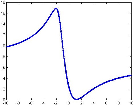
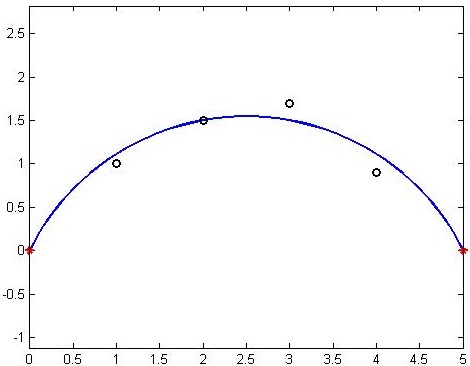
In the following page, there is a simple example of the function f๐‘“f and the related least square arc.

3 Searching longest arcs

In this section we want to explain how to apply least square constrained arcs in the approximation of a planar data set without corners (we suppose that the profile of our object is locally smooth). Suppose that ๐1,๐2,โ€ฆ,๐Nsubscript๐1subscript๐2โ€ฆsubscript๐๐‘\mathbf{P}_{1},\mathbf{P}_{2},\dots,\mathbf{P}_{N} are N๐‘N consecutive points approximating one section of the object contour.
Refer to caption
Refer to caption
Figure 1: Example of least square constrained arc passing through (0,0),ย (5,0) (on the left) and the relative function f๐‘“f (on the right).

The first step of the method consists in trying to approximate the first four points with a constrained arc (it starts from four because we already know that there always exists one arc passing through three points, eventually with infinite radius). We decide an error limit and we compute the distance of each point ๐ksubscript๐๐‘˜\mathbf{P}_{k} from the arc. If there exists one point whose distance is greater than our limit, we decrease the number of approximated points and, in this case, we build the arc passing through the first three points. Conversely, if all the points are within the error limit, we increase the number of approximated points and we try to build a longer arc. The method repeats these steps for each point ๐k,k=1,2,โ€ฆ,Nโˆ’2formulae-sequencesubscript๐๐‘˜๐‘˜12โ€ฆ๐‘2\mathbf{P}_{k},k=1,2,\dots,N-2. At the end we obtain a Nร—1๐‘1N\times 1 matrix M๐‘€M: in the ktโ€‹hsuperscript๐‘˜๐‘กโ„Žk^{th} place there will be the number of points that can be approximated with a single least square arc starting from ๐ksubscript๐๐‘˜\mathbf{P}_{k} โ€” included the first and the last points โ€”. We will set Mโ€‹(Nโˆ’1)=Mโ€‹(N)=0๐‘€๐‘1๐‘€๐‘0M(N-1)=M(N)=0. Here follows the algorithm (which needs at least four points in order to be applied):

  1. 1.

    Set i=1,k=3,fโ€‹lโ€‹aโ€‹g=1formulae-sequence๐‘–1formulae-sequence๐‘˜3๐‘“๐‘™๐‘Ž๐‘”1i=1,\ k=3,\ flag=1 and choose ฮต>0๐œ€0\varepsilon>0;

  2. 2.

    While iโ‰คNโˆ’2๐‘–๐‘2i\leq N-2 do

  3. 3.

    Set l=kโˆ’1๐‘™๐‘˜1l=k-1;

  4. 4.

    Find the center ๐‚๐‚\mathbf{C} and the radius R๐‘…R

    of the least square arc passing

    through ๐isubscript๐๐‘–\mathbf{P}_{i}, ๐i+ksubscript๐๐‘–๐‘˜\mathbf{P}_{i+k};

  5. 5.

    For j=1,โ€ฆ,l๐‘—1โ€ฆ๐‘™j=1,\dots,l

  6. 6.

    d=โˆฃRโˆ’โ€–๐i+jโˆ’๐‚โ€–โˆฃ๐‘‘delimited-โˆฃโˆฃ๐‘…normsubscript๐๐‘–๐‘—๐‚d=\ \mid R-\parallel\mathbf{P}_{i+j}-\mathbf{C}\parallel\mid;

  7. 7.

    If d>ฮต๐‘‘๐œ€d>\varepsilon set fโ€‹lโ€‹aโ€‹g=0๐‘“๐‘™๐‘Ž๐‘”0flag=0; break;

  8. 8.

    If fโ€‹lโ€‹aโ€‹g=0๐‘“๐‘™๐‘Ž๐‘”0flag=0

  9. 9.

    build the least square arc

    passing through ๐isubscript๐๐‘–\mathbf{P}_{i}, ๐i+kโˆ’1subscript๐๐‘–๐‘˜1\mathbf{P}_{i+k-1}

  10. 10.

    Mโ€‹(i)=k๐‘€๐‘–๐‘˜M(i)=k, fโ€‹lโ€‹aโ€‹g=1๐‘“๐‘™๐‘Ž๐‘”1flag=1, i=i+1๐‘–๐‘–1i=i+1;

  11. 11.

    If i=Nโˆ’2๐‘–๐‘2i=N-2 set k=2๐‘˜2k=2

    Else set k=3๐‘˜3k=3;

    Else

  12. 12.

    k=k+1๐‘˜๐‘˜1k=k+1;

  13. 13.

    If i+k>N๐‘–๐‘˜๐‘i+k>N

  14. 14.

    build the least square

    arc passing through

    ๐isubscript๐๐‘–\mathbf{P}_{i}, ๐i+kโˆ’1subscript๐๐‘–๐‘˜1\mathbf{P}_{i+k-1}

  15. 15.

    Mโ€‹(i)=k๐‘€๐‘–๐‘˜M(i)=k, i=i+1๐‘–๐‘–1i=i+1;

  16. 16.

    If i=Nโˆ’2๐‘–๐‘2i=N-2 set k=2๐‘˜2k=2

    Else set k=3๐‘˜3k=3;

  17. 17.

    Mโ€‹(Nโˆ’1)=0,Mโ€‹(N)=0formulae-sequence๐‘€๐‘10๐‘€๐‘0M(N-1)=0,\ M(N)=0.

One can notice that Mโ€‹(k)โ‰ฅ3๐‘€๐‘˜3M(k)\geq 3 for all k=1,โ€ฆ,Nโˆ’2๐‘˜1โ€ฆ๐‘2k=1,\dots,N-2, so that the worst case occurs when all the elements of M๐‘€M are equal to three. Next step is to decide how to choose the longest arcs.

4 Selection of longest arcs

We will explain the choice of longest arcs with two simple examples. Fix kโ‰ฅ1๐‘˜1k\geq 1 and suppose that Mโ€‹(k)=n๐‘€๐‘˜๐‘›M(k)=n, for a certain nโ‰ฅ3โˆˆโ„•๐‘›3โ„•n\geq 3\in\mathds{N}. Suppose also that Mโ€‹(i)<Mโ€‹(k)๐‘€๐‘–๐‘€๐‘˜M(i)<M(k) for all i=k+1,k+2,โ€ฆ,k+nโˆ’1๐‘–๐‘˜1๐‘˜2โ€ฆ๐‘˜๐‘›1i=k+1,k+2,\dots,k+n-1. This is the simplest case: the arc starting from ๐ksubscript๐๐‘˜\mathbf{P}_{k} is approximating an higher number of points than the nโˆ’1๐‘›1n-1 consecutive arcs, so it is good for an optimized approximation. Now suppose that an index j๐‘—j exists such that 1โ‰คjโ‰คnโˆ’11๐‘—๐‘›11\leq j\leq n-1 and Mโ€‹(k+j)>Mโ€‹(k)๐‘€๐‘˜๐‘—๐‘€๐‘˜M(k+j)>M(k). In this situation we canโ€™t say that the arc starting from ๐ksubscript๐๐‘˜\mathbf{P}_{k} is the best for our task. Let

S=โŒŠMโ€‹(k)2โŒ‹๐‘†๐‘€๐‘˜2S=\bigg{\lfloor}\frac{M(k)}{2}\bigg{\rfloor}

and let Iksubscript๐ผ๐‘˜I_{k} be the set

Ik={jโˆˆโ„•|k+1โ‰คjโ‰คk+S}.subscript๐ผ๐‘˜conditional-set๐‘—โ„•๐‘˜1๐‘—๐‘˜๐‘†I_{k}=\{j\in\mathds{N}\ |\ k+1\leq j\leq k+S\}.

Then, we decide to apply the following test: if Mโ€‹(j)โ‰คMโ€‹(k)๐‘€๐‘—๐‘€๐‘˜M(j)\leq M(k) for all jโˆˆIk๐‘—subscript๐ผ๐‘˜j\in I_{k}, the arc starting from ๐ksubscript๐๐‘˜\mathbf{P}_{k} is good for our approximation and we pass from ๐ksubscript๐๐‘˜\mathbf{P}_{k} to ๐k+Mโ€‹(k)โˆ’1subscript๐๐‘˜๐‘€๐‘˜1\mathbf{P}_{k+M(k)-1} with a single arc. We repeat the process on ๐k+Mโ€‹(k)โˆ’1subscript๐๐‘˜๐‘€๐‘˜1\mathbf{P}_{k+M(k)-1} (the new starting point). Conversely, if an index jโˆˆIk๐‘—subscript๐ผ๐‘˜j\in I_{k} exists such that Mโ€‹(j)>Mโ€‹(k)๐‘€๐‘—๐‘€๐‘˜M(j)>M(k) we pass directly from the point ๐ksubscript๐๐‘˜\mathbf{P}_{k} to ๐jsubscript๐๐‘—\mathbf{P}_{j} without any segments or arcs โ€” for the moment โ€” and we apply again the test on the new starting point ๐jsubscript๐๐‘—\mathbf{P}_{j}. This kind of selection is justified by the following fact: suppose there exists an index jโˆ‰Ik๐‘—subscript๐ผ๐‘˜j\notin I_{k} such that Mโ€‹(j)>Mโ€‹(k)๐‘€๐‘—๐‘€๐‘˜M(j)>M(k) and Mโ€‹(k)๐‘€๐‘˜M(k) is a high number (Mโ€‹(k)โ‰ฅ20๐‘€๐‘˜20M(k)\geq 20 for example ); then, the gap between ๐ksubscript๐๐‘˜\mathbf{P}_{k} and ๐jsubscript๐๐‘—\mathbf{P}_{j} can be so wide that we are not able to obtain a good approximation for all those points among them, so the test is applied only on the set Iksubscript๐ผ๐‘˜I_{k}.

Here follows the algorithm (N๐‘N is, as usual, the number of points we are approximating):

  1. 1.

    Set i=1๐‘–1i=1, G=M๐บ๐‘€G=M;

  2. 2.

    While i<N๐‘–๐‘i<N do

  3. 3.

    S=โŒŠMโ€‹(i)2โŒ‹๐‘†๐‘€๐‘–2S=\bigg{\lfloor}\frac{M(i)}{2}\bigg{\rfloor}, j=i+1๐‘—๐‘–1j=i+1, fโ€‹lโ€‹aโ€‹g=1๐‘“๐‘™๐‘Ž๐‘”1flag=1,

    e=i+Mโ€‹(i)โˆ’1๐‘’๐‘–๐‘€๐‘–1e=i+M(i)-1;

  4. 4.

    While jโ‰คi+S๐‘—๐‘–๐‘†j\leq i+S and fโ€‹lโ€‹aโ€‹g=1๐‘“๐‘™๐‘Ž๐‘”1flag=1 do

  5. 5.

    If Mโ€‹(j)โ‰คMโ€‹(i)๐‘€๐‘—๐‘€๐‘–M(j)\leq M(i) set j=j+1๐‘—๐‘—1j=j+1

    Else

  6. 6.

    Set fโ€‹lโ€‹aโ€‹g=0๐‘“๐‘™๐‘Ž๐‘”0flag=0;

  7. 7.

    for k=i,โ€ฆ,jโˆ’1๐‘˜๐‘–โ€ฆ๐‘—1k=i,\dots,j-1

    set Gโ€‹(k)=0๐บ๐‘˜0G(k)=0;

  8. 8.

    Set i=j๐‘–๐‘—i=j;

    e=i+Mโ€‹(i)โˆ’1๐‘’๐‘–๐‘€๐‘–1e=i+M(i)-1; break;

  9. 9.

    If fโ€‹lโ€‹aโ€‹g=1๐‘“๐‘™๐‘Ž๐‘”1flag=1

  10. 10.

    For k=i+1,โ€ฆ,eโˆ’1๐‘˜๐‘–1โ€ฆ๐‘’1k=i+1,\dots,e-1

    Gโ€‹(k)=0๐บ๐‘˜0G(k)=0;

  11. 11.

    Set i=e๐‘–๐‘’i=e;

In this algorithm we introduce a new matrix G๐บG. At the beginning, G๐บG is equal to M๐‘€M, but during the steps the element Gโ€‹(i)๐บ๐‘–G(i) may become null. This happens in two cases, if ๐ksubscript๐๐‘˜\mathbf{P}_{k} is a starting point:

  • โ€ข

    Mโ€‹(k)โ‰ฅMโ€‹(j)๐‘€๐‘˜๐‘€๐‘—M(k)\geq M(j) for all jโˆˆIk๐‘—subscript๐ผ๐‘˜j\in I_{k}. Then we set Gโ€‹(j)=0๐บ๐‘—0G(j)=0 for all j๐‘—j such that k+1โ‰คjโ‰คk+Mโ€‹(k)โˆ’2๐‘˜1๐‘—๐‘˜๐‘€๐‘˜2k+1\leq j\leq k+M(k)-2;

  • โ€ข

    there exists some index jโˆˆIk๐‘—subscript๐ผ๐‘˜j\in I_{k} such that Mโ€‹(k)<Mโ€‹(j)๐‘€๐‘˜๐‘€๐‘—M(k)<M(j). Then we set Gโ€‹(i)=0๐บ๐‘–0G(i)=0 for all iโˆˆIk๐‘–subscript๐ผ๐‘˜i\in I_{k} satisfying k+1โ‰คiโ‰คjโˆ’1๐‘˜1๐‘–๐‘—1k+1\leq i\leq j-1 and for i=k๐‘–๐‘˜i=k.

At the end of the process we obtain a Nร—1๐‘1N\times 1 matrix G๐บG with elements Gโ€‹(k)๐บ๐‘˜G(k) satisfying:

  • โ‹„โ‹„\diamond

    Gโ€‹(k)>0๐บ๐‘˜0G(k)>0, if there exists a single arc passing through the points ๐ksubscript๐๐‘˜\mathbf{P}_{k}, ๐k+Gโ€‹(k)โˆ’1subscript๐๐‘˜๐บ๐‘˜1\mathbf{P}_{k+G(k)-1} and approximating all the other points among them, i.e. if the point ๐ksubscript๐๐‘˜\mathbf{P}_{k} is a starting point for one arc;

  • โ‹„โ‹„\diamond

    Gโ€‹(k)=0๐บ๐‘˜0G(k)=0, if the point ๐ksubscript๐๐‘˜\mathbf{P}_{k} is not a starting point, so Gโ€‹(Nโˆ’1)=Gโ€‹(N)=0๐บ๐‘1๐บ๐‘0G(N-1)=G(N)=0.

Suppose now Gโ€‹(k)>0๐บ๐‘˜0G(k)>0 and Gโ€‹(k+Gโ€‹(k)โˆ’1)>0๐บ๐‘˜๐บ๐‘˜10G(k+G(k)-1)>0: then there exist two consecutive arcs (continous arcs) with common point ๐k+Gโ€‹(k)โˆ’1subscript๐๐‘˜๐บ๐‘˜1\mathbf{P}_{k+G(k)-1}. This is the best case: all points between ๐ksubscript๐๐‘˜\mathbf{P}_{k} and ๐k+Gโ€‹(k)โˆ’1+Gโ€‹(k+Gโ€‹(k)โˆ’1)โˆ’1subscript๐๐‘˜๐บ๐‘˜1๐บ๐‘˜๐บ๐‘˜11\mathbf{P}_{k+G(k)-1+G(k+G(k)-1)-1} are approximated within the tolerance. But what happens when two consecutive arcs donโ€™t have a common point? This is the next step: how to fill the gaps between the built arcs.

5 Constrained Biarcs

Before proceeding to the next step, we want to discuss about biarcs and their applications.

Definition 5.1.

We say that two circular arcs a1subscript๐‘Ž1a_{1}, a2subscript๐‘Ž2a_{2} form a constrained biarc passing through given points ๐ssubscript๐๐‘ \mathbf{P}_{s}, ๐esubscript๐๐‘’\mathbf{P}_{e} with unit tangent vectors ๐“ssubscript๐“๐‘ \mathbf{T}_{s}, ๐“esubscript๐“๐‘’\mathbf{T}_{e}, if they have a common point ๐2subscript๐2\mathbf{P}_{2} satisfying the following properties:

  • โˆ—โˆ—\ast

    a1subscript๐‘Ž1a_{1} starts from ๐ssubscript๐๐‘ \mathbf{P}_{s}, ends in ๐2subscript๐2\mathbf{P}_{2} and ๐“ssubscript๐“๐‘ \mathbf{T}_{s} is tangent to a1subscript๐‘Ž1a_{1} in ๐1subscript๐1\mathbf{P}_{1}, with orientation corresponding to a parametrization of a1subscript๐‘Ž1a_{1} from ๐ssubscript๐๐‘ \mathbf{P}_{s} to ๐2subscript๐2\mathbf{P}_{2};

  • โˆ—โˆ—\ast

    a2subscript๐‘Ž2a_{2} starts from ๐2subscript๐2\mathbf{P}_{2}, ends in ๐esubscript๐๐‘’\mathbf{P}_{e} and ๐“esubscript๐“๐‘’\mathbf{T}_{e} is tangent to a2subscript๐‘Ž2a_{2} in ๐esubscript๐๐‘’\mathbf{P}_{e}, with orientation corresponding to a parametrization of a2subscript๐‘Ž2a_{2} from ๐2subscript๐2\mathbf{P}_{2} to ๐esubscript๐๐‘’\mathbf{P}_{e};

  • โˆ—โˆ—\ast

    a1subscript๐‘Ž1a_{1} and a2subscript๐‘Ž2a_{2} have proportional tangent vectors in ๐2subscript๐2\mathbf{P}_{2} (i.e. the biarc is G1superscript๐บ1G^{1} continous in ๐2subscript๐2\mathbf{P}_{2}).

In this paper we will use the standard notation used by Piegl and Tiller in [7], [8]. The control points of the biarc are determined by

๐1=๐s+ฮฑโ€‹๐“s,subscript๐1subscript๐๐‘ ๐›ผsubscript๐“๐‘ \mathbf{P}_{1}=\mathbf{P}_{s}+\alpha\mathbf{T}_{s},
๐3=๐eโˆ’ฮฒโ€‹๐“e,subscript๐3subscript๐๐‘’๐›ฝsubscript๐“๐‘’\mathbf{P}_{3}=\mathbf{P}_{e}-\beta\mathbf{T}_{e},

with both ฮฑ๐›ผ\alpha and ฮฒ๐›ฝ\beta positive. Using this convention, the sweep angle of each arc of the biarc will always be in [0,ฯ€)0๐œ‹[0,\pi). Now, let ๐•=๐eโˆ’๐s๐•subscript๐๐‘’subscript๐๐‘ \mathbf{V}=\mathbf{P}_{e}-\mathbf{P}_{s}. We will prove that there always exists a biarc passing through ๐ssubscript๐๐‘ \mathbf{P}_{s}, ๐esubscript๐๐‘’\mathbf{P}_{e} when

๐“sโ‹…๐“eโ‰ 1โ‹…subscript๐“๐‘ subscript๐“๐‘’1\mathbf{T}_{s}\cdot\mathbf{T}_{e}\neq 1 (11)

and

๐•โ‹…๐•โ‰ 2โ€‹(๐•โ‹…๐“s)โ€‹(๐•โ‹…๐“e)๐“sโ‹…๐“eโˆ’1.โ‹…๐•๐•2โ‹…๐•subscript๐“๐‘ โ‹…๐•subscript๐“๐‘’โ‹…subscript๐“๐‘ subscript๐“๐‘’1\mathbf{V}\cdot\mathbf{V}\neq\frac{2(\mathbf{V}\cdot\mathbf{T}_{s})(\mathbf{V}\cdot\mathbf{T}_{e})}{\mathbf{T}_{s}\cdot\mathbf{T}_{e}-1}. (12)
Theorem 5.1.

Given two distinct planar points ๐ssubscript๐๐‘ \mathbf{P}_{s}, ๐esubscript๐๐‘’\mathbf{P}_{e} with associated unit vectors ๐“ssubscript๐“๐‘ \mathbf{T}_{s}, ๐“esubscript๐“๐‘’\mathbf{T}_{e} satisfying (11) and (12), there always exists a biarc passing through ๐ssubscript๐๐‘ \mathbf{P}_{s}, ๐esubscript๐๐‘’\mathbf{P}_{e} with tangents ๐“ssubscript๐“๐‘ \mathbf{T}_{s}, ๐“esubscript๐“๐‘’\mathbf{T}_{e}.

Proof.

Let ๐1=๐s+ฮฑโ€‹๐“ssubscript๐1subscript๐๐‘ ๐›ผsubscript๐“๐‘ \mathbf{P}_{1}=\mathbf{P}_{s}+\alpha\mathbf{T}_{s}, with ฮฑ>0๐›ผ0\alpha>0. Then itโ€™s sufficient to prove that there exists a point ๐3subscript๐3\mathbf{P}_{3} such that ๐3=๐eโˆ’ฮฒโ€‹๐“esubscript๐3subscript๐๐‘’๐›ฝsubscript๐“๐‘’\mathbf{P}_{3}=\mathbf{P}_{e}-\beta\mathbf{T}_{e}, ฮฒ>0๐›ฝ0\beta>0, and โ€–๐3โˆ’๐1โ€–=ฮฑ+ฮฒnormsubscript๐3subscript๐1๐›ผ๐›ฝ\parallel\mathbf{P}_{3}-\mathbf{P}_{1}\parallel=\alpha+\beta. This is equivalent to the condition

(๐3โˆ’๐1)โ‹…(๐3โˆ’๐1)=(ฮฑ+ฮฒ)2.โ‹…subscript๐3subscript๐1subscript๐3subscript๐1superscript๐›ผ๐›ฝ2(\mathbf{P}_{3}-\mathbf{P}_{1})\cdot(\mathbf{P}_{3}-\mathbf{P}_{1})={(\alpha+\beta)}^{2}.

Substituting the values of ๐1subscript๐1\mathbf{P}_{1}, ๐3subscript๐3\mathbf{P}_{3}, we find the condition

(๐•โˆ’ฮฑโ€‹๐“sโˆ’ฮฒโ€‹๐“e)โ‹…(๐•โˆ’ฮฑโ€‹๐“sโˆ’ฮฒโ€‹๐“e)=(ฮฑ+ฮฒ)2.โ‹…๐•๐›ผsubscript๐“๐‘ ๐›ฝsubscript๐“๐‘’๐•๐›ผsubscript๐“๐‘ ๐›ฝsubscript๐“๐‘’superscript๐›ผ๐›ฝ2(\mathbf{V}-\alpha\mathbf{T}_{s}-\beta\mathbf{T}_{e})\cdot(\mathbf{V}-\alpha\mathbf{T}_{s}-\beta\mathbf{T}_{e})={(\alpha+\beta)}^{2}.

Expliciting the products, we find

๐•โ‹…๐•โˆ’2โ€‹ฮฑโ€‹๐•โ‹…๐“sโˆ’2โ€‹ฮฒโ€‹๐•โ‹…๐“e+2โ€‹ฮฑโ€‹ฮฒโ€‹(๐“sโ‹…๐“eโˆ’1)=0.โ‹…๐•๐•โ‹…2๐›ผ๐•subscript๐“๐‘ โ‹…2๐›ฝ๐•subscript๐“๐‘’2๐›ผ๐›ฝโ‹…subscript๐“๐‘ subscript๐“๐‘’10\mathbf{V}\cdot\mathbf{V}-2\alpha\mathbf{V}\cdot\mathbf{T}_{s}-2\beta\mathbf{V}\cdot\mathbf{T}_{e}+2\alpha\beta(\mathbf{T}_{s}\cdot\mathbf{T}_{e}-1)=0.

So, expliciting ฮฒ๐›ฝ\beta:

ฮฒ=2โ€‹ฮฑโ€‹๐•โ‹…๐“sโˆ’๐•โ‹…๐•2โ€‹ฮฑโ€‹(๐“sโ‹…๐“eโˆ’1)โˆ’2โ€‹๐•โ‹…๐“e.๐›ฝโ‹…2๐›ผ๐•subscript๐“๐‘ โ‹…๐•๐•2๐›ผโ‹…subscript๐“๐‘ subscript๐“๐‘’1โ‹…2๐•subscript๐“๐‘’\beta=\frac{2\alpha\mathbf{V}\cdot\mathbf{T}_{s}-\mathbf{V}\cdot\mathbf{V}}{2\alpha(\mathbf{T}_{s}\cdot\mathbf{T}_{e}-1)-2\mathbf{V}\cdot\mathbf{T}_{e}}. (13)

Now, assume that exists ฮฑ>0๐›ผ0\alpha>0 such that ฮฒ>0๐›ฝ0\beta>0. Then, one can define the junction point ๐2subscript๐2\mathbf{P}_{2} as

๐2=ฮฒฮฑ+ฮฒโ€‹๐1+ฮฑฮฑ+ฮฒโ€‹๐3.subscript๐2๐›ฝ๐›ผ๐›ฝsubscript๐1๐›ผ๐›ผ๐›ฝsubscript๐3\mathbf{P}_{2}=\frac{\beta}{\alpha+\beta}\mathbf{P}_{1}+\frac{\alpha}{\alpha+\beta}\mathbf{P}_{3}.

Since โ€–๐2โˆ’๐1โ€–=ฮฑnormsubscript๐2subscript๐1๐›ผ\parallel\mathbf{P}_{2}-\mathbf{P}_{1}\parallel=\alpha and โ€–๐3โˆ’๐2โ€–=ฮฒnormsubscript๐3subscript๐2๐›ฝ\parallel\mathbf{P}_{3}-\mathbf{P}_{2}\parallel=\beta, we can build two arcs c1subscript๐‘1c_{1}, c2subscript๐‘2c_{2} satisfying the conditions of the Definition 5.1. โˆŽ

The proof of the theorem uses the following

Lemma 5.1.

Given two distinct planar points ๐ssubscript๐๐‘ \mathbf{P}_{s}, ๐esubscript๐๐‘’\mathbf{P}_{e} with associated unit vectors ๐“ssubscript๐“๐‘ \mathbf{T}_{s}, ๐“esubscript๐“๐‘’\mathbf{T}_{e} satisfying [11] and [12], there always exists a positive value of ฮฑ๐›ผ\alpha such that ฮฒ>0๐›ฝ0\beta>0, where ฮฒ๐›ฝ\beta is defined in equation [13].

Proof.

Let

ฮฑ1=๐•โ‹…๐•2โ€‹๐•โ‹…๐“s,ฮฑ2=๐•โ‹…๐“e๐“sโ‹…๐“eโˆ’1,formulae-sequencesubscript๐›ผ1โ‹…๐•๐•โ‹…2๐•subscript๐“๐‘ subscript๐›ผ2โ‹…๐•subscript๐“๐‘’โ‹…subscript๐“๐‘ subscript๐“๐‘’1\alpha_{1}=\frac{\mathbf{V}\cdot\mathbf{V}}{2\mathbf{V}\cdot\mathbf{T}_{s}},\ \alpha_{2}=\frac{\mathbf{V}\cdot\mathbf{T}_{e}}{\mathbf{T}_{s}\cdot\mathbf{T}_{e}-1},
K=๐•โ‹…๐“s๐“sโ‹…๐“eโˆ’1.๐พโ‹…๐•subscript๐“๐‘ โ‹…subscript๐“๐‘ subscript๐“๐‘’1K=\frac{\mathbf{V}\cdot\mathbf{T}_{s}}{\mathbf{T}_{s}\cdot\mathbf{T}_{e}-1}.

Then, by hypothesis, ฮฑ1โ‰ ฮฑ2subscript๐›ผ1subscript๐›ผ2\alpha_{1}\neq\alpha_{2}. From equation (13) we can write

ฮฒ=Kโ€‹ฮฑโˆ’ฮฑ1ฮฑโˆ’ฮฑ2.๐›ฝ๐พ๐›ผsubscript๐›ผ1๐›ผsubscript๐›ผ2\beta=K\frac{\alpha-\alpha_{1}}{\alpha-\alpha_{2}}.

There are three cases to be examined.

  • โˆ™โˆ™\bullet

    K > 0. We have ๐•โ‹…๐“s<0โ‹…๐•subscript๐“๐‘ 0\mathbf{V}\cdot\mathbf{T}_{s}<0, so ฮฑ1<0subscript๐›ผ10\alpha_{1}<0 and ฮฒ๐›ฝ\beta is positive for ฮฑ>maxโ€‹{ฮฑ2,0}๐›ผmaxsubscript๐›ผ20\alpha>\text{max}\{\alpha_{2},0\}. Notice that if ฮฑ1=ฮฑ2subscript๐›ผ1subscript๐›ผ2\alpha_{1}=\alpha_{2} one obtains ฮฒโ‰กK>0๐›ฝ๐พ0\beta\equiv K>0 regardless ฮฑ๐›ผ\alpha. In this case one arc of the biarc is degenerate (a segment), but the theorem doesnโ€™t concern this situation.

  • โˆ™โˆ™\bullet

    K < 0. We have ๐•โ‹…๐“s>0โ‹…๐•subscript๐“๐‘ 0\mathbf{V}\cdot\mathbf{T}_{s}>0, so ฮฑ1>0subscript๐›ผ10\alpha_{1}>0. There are three subcases:

    • โ€“

      ฮฑ2โ‰ค0<ฮฑ1subscript๐›ผ20subscript๐›ผ1\alpha_{2}\leq 0<\alpha_{1}. We choose ฮฑโˆˆ(0,ฮฑ1)๐›ผ0subscript๐›ผ1\alpha\in(0,\alpha_{1});

    • โ€“

      0<ฮฑ1<ฮฑ20subscript๐›ผ1subscript๐›ผ20<\alpha_{1}<\alpha_{2}. We choose ฮฑโˆˆ(ฮฑ1,ฮฑ2)๐›ผsubscript๐›ผ1subscript๐›ผ2\alpha\in(\alpha_{1},\alpha_{2});

    • โ€“

      0โ‰คฮฑ2<ฮฑ10subscript๐›ผ2subscript๐›ผ10\leq\alpha_{2}<\alpha_{1}. We choose ฮฑโˆˆ(ฮฑ2,ฮฑ1)๐›ผsubscript๐›ผ2subscript๐›ผ1\alpha\in(\alpha_{2},\alpha_{1}).

  • โˆ™โˆ™\bullet

    K = 0. We have ๐•โ‹…๐“s=0โ‹…๐•subscript๐“๐‘ 0\mathbf{V}\cdot\mathbf{T}_{s}=0, so

    ฮฒ=โˆ’๐•โ‹…๐•2โ€‹(๐“sโ‹…๐“eโˆ’1)โ€‹(ฮฑโˆ’ฮฑ2).๐›ฝโ‹…๐•๐•2โ‹…subscript๐“๐‘ subscript๐“๐‘’1๐›ผsubscript๐›ผ2\beta=\frac{-\mathbf{V}\cdot\mathbf{V}}{2(\mathbf{T}_{s}\cdot\mathbf{T}_{e}-1)(\alpha-\alpha_{2})}.

    We choose ฮฑ>maxโ€‹{ฮฑ2,0}๐›ผmaxsubscript๐›ผ20\alpha>\text{max}\{\alpha_{2},0\}.

โˆŽ

The condition of the lemma

๐•โ‹…๐•โ‰ 2โ€‹(๐•โ‹…๐“s)โ€‹(๐•โ‹…๐“e)๐“sโ‹…๐“eโˆ’1โ‹…๐•๐•2โ‹…๐•subscript๐“๐‘ โ‹…๐•subscript๐“๐‘’โ‹…subscript๐“๐‘ subscript๐“๐‘’1\mathbf{V}\cdot\mathbf{V}\neq\frac{2(\mathbf{V}\cdot\mathbf{T}_{s})(\mathbf{V}\cdot\mathbf{T}_{e})}{\mathbf{T}_{s}\cdot\mathbf{T}_{e}-1} (14)

can be read in a geometrical way. Let ฮธ1subscript๐œƒ1\theta_{1}, ฮธ2subscript๐œƒ2\theta_{2}, ฮธ3subscript๐œƒ3\theta_{3} be respectively the angles between (๐•,๐“s)๐•subscript๐“๐‘ (\mathbf{V},\mathbf{T}_{s}), (๐•,๐“e)๐•subscript๐“๐‘’(\mathbf{V},\mathbf{T}_{e}), (๐“s,๐“e)subscript๐“๐‘ subscript๐“๐‘’(\mathbf{T}_{s},\mathbf{T}_{e}). Then, from (14), we find

โ€–๐•โ€–2โ‰ 2โ€‹โ€–๐•โ€–2โ€‹cosโกฮธ1โ€‹cosโกฮธ2cosโกฮธ3โˆ’1,superscriptnorm๐•22superscriptnorm๐•2subscript๐œƒ1subscript๐œƒ2subscript๐œƒ31{\parallel\mathbf{V}\parallel}^{2}\neq 2\frac{{\parallel\mathbf{V}\parallel}^{2}\cos{\theta_{1}}\cos{\theta_{2}}}{\cos{\theta_{3}}-1},

or, simplifying,

cosโกฮธ3โ‰ 2โ€‹cosโกฮธ1โ€‹cosโกฮธ2+1.subscript๐œƒ32subscript๐œƒ1subscript๐œƒ21\cos{\theta_{3}}\neq 2\cos{\theta_{1}}\cos{\theta_{2}}+1. (15)

Itโ€™s easy to see that a necessary condition to have cosโกฮธ3=2โ€‹cosโกฮธ1โ€‹cosโกฮธ2+1subscript๐œƒ32subscript๐œƒ1subscript๐œƒ21\cos{\theta_{3}}=2\cos{\theta_{1}}\cos{\theta_{2}}+1 is that โˆ’1โ‰คcosโกฮธ1โ€‹cosโกฮธ2โ‰ค01subscript๐œƒ1subscript๐œƒ20-1\leq\cos{\theta_{1}}\cos{\theta_{2}}\leq 0. The condition (15) includes many cases, but in all of these situations one can solve the connection problem using two consecutive biarcs. Clearly, things get simpler when ฮฑ=ฮฒ๐›ผ๐›ฝ\alpha=\beta. In this situation, there are only two cases in which we canโ€™t build a single arc: ๐“sโ‹…๐“e=1โ‹…subscript๐“๐‘ subscript๐“๐‘’1\mathbf{T}_{s}\cdot\mathbf{T}_{e}=1 and ๐•โ‹…(๐“s+๐“e)=0โ‹…๐•subscript๐“๐‘ subscript๐“๐‘’0\mathbf{V}\cdot(\mathbf{T}_{s}+\mathbf{T}_{e})=0. In both cases we have to build two consecutive biarcs, i.e. four arcs, matching with G1superscript๐บ1G^{1} continuity. In general, one can define the biarc ratio r=ฮฑฮฒ๐‘Ÿ๐›ผ๐›ฝr=\frac{\alpha}{\beta} instead of choosing a value of ฮฑ๐›ผ\alpha to have ฮฒ>0๐›ฝ0\beta>0.

Refer to caption
Refer to caption
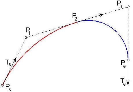
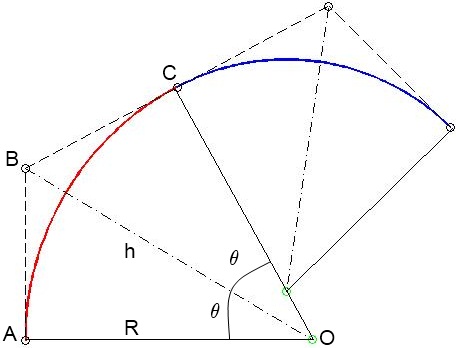
Figure 2: Example of constrained biarc passing through ๐s=(0,0)subscript๐๐‘ 00\mathbf{P}_{s}=(0,0), ๐e=(5,1)subscript๐๐‘’51\mathbf{P}_{e}=(5,1) with tangent vectors ๐“s=(1,1)subscript๐“๐‘ 11\mathbf{T}_{s}=(1,1), ๐“e=(0,โˆ’1)subscript๐“๐‘’01\mathbf{T}_{e}=(0,-1) (on the left) and construction of a biarc (on the right).

The ratio r๐‘Ÿr is very useful when we want to build a constrained biarc minimizing the distance from given planar points. An efficient algorithm has been studied by Hyungjun Park in [5]: itโ€™s called optimal single biarc fitting, and its approach is to search an optimized value of r๐‘Ÿr decreasing the width of the range of r๐‘Ÿr in each step. We will use this approach in the next steps.

6 Biarcs in Bรฉzier form

Let us consider the biarc in Figure 2 (on the right). Let ๐š๐›=๐โˆ’๐€โ€–๐โˆ’๐€โ€–๐š๐›๐๐€norm๐๐€\mathbf{ab}=\frac{\mathbf{B}-\mathbf{A}}{\|\mathbf{B}-\mathbf{A}\|}, ๐›๐œ=๐‚โˆ’๐โ€–๐‚โˆ’๐โ€–๐›๐œ๐‚๐norm๐‚๐\mathbf{bc}=\frac{\mathbf{C}-\mathbf{B}}{\|\mathbf{C}-\mathbf{B}\|}. Then we have

D=(๐š๐›,๐›๐œ)=cosโก2โ€‹ฮธ,๐ท๐š๐›๐›๐œ2๐œƒD=(\mathbf{ab},\mathbf{bc})=\cos{2\theta},

where ฮธ๐œƒ\theta is the half sweep angle of the biarc, and we suppose that ฮธโˆˆ[0,ฯ€2)๐œƒ0๐œ‹2\theta\in\big{[}0,\frac{\pi}{2}\big{)}. By bisection formulas one can find

cosโกฮธ=1+D2,sinโกฮธ=1โˆ’D2,tanโกฮธ=1โˆ’D1+D.formulae-sequence๐œƒ1๐ท2formulae-sequence๐œƒ1๐ท2๐œƒ1๐ท1๐ท\begin{split}\cos{\theta}=\sqrt{\frac{1+D}{2}},&\ \sin{\theta}=\sqrt{\frac{1-D}{2}},\\ \tan{\theta}=&\sqrt{\frac{1-D}{1+D}}.\end{split} (16)

So the explicit formula for ฮธ๐œƒ\theta becomes

ฮธ=arctanโก1โˆ’D1+D.๐œƒ1๐ท1๐ท\theta=\arctan{\sqrt{\frac{1-D}{1+D}}}.

Since R=hโ€‹cosโกฮธ๐‘…โ„Ž๐œƒR=h\cos{\theta} and โ€–๐โˆ’๐€โ€–=hโ€‹sinโกฮธnorm๐๐€โ„Ž๐œƒ\|\mathbf{B}-\mathbf{A}\|=h\sin{\theta} we can find the radius and the centre of the first arc:

R=1+D1โˆ’Dโ€‹โ€–๐โˆ’๐€โ€–,๐Ž=๐+Rcosโกฮธโ€‹๐š๐›โˆ’๐›๐œโ€–๐š๐›โˆ’๐›๐œโ€–.formulae-sequence๐‘…1๐ท1๐ทdelimited-โˆฅโˆฅ๐๐€๐Ž๐๐‘…๐œƒ๐š๐›๐›๐œnorm๐š๐›๐›๐œ\begin{split}R=&\sqrt{\frac{1+D}{1-D}}\|\mathbf{B}-\mathbf{A}\|,\\ \mathbf{O}=&\mathbf{B}+\frac{R}{\cos{\theta}}\frac{\mathbf{ab}-\mathbf{bc}}{\|\mathbf{ab}-\mathbf{bc}\|}.\end{split} (17)

Suppose ๐0=๐€subscript๐0๐€\mathbf{P}_{0}=\mathbf{A}, ๐1=๐subscript๐1๐\mathbf{P}_{1}=\mathbf{B}, ๐2=๐‚subscript๐2๐‚\mathbf{P}_{2}=\mathbf{C} and {w0,w1,w2}={1,cosโกฮธ,1}subscript๐‘ค0subscript๐‘ค1subscript๐‘ค21๐œƒ1\{w_{0},w_{1},w_{2}\}=\{1,\cos{\theta},1\}. Then we easily obtain the parametrization of the first arc:

๐†โ€‹(t)=โˆ‘i=02wiโ€‹๐iโ€‹Bi2โ€‹(t)โˆ‘i=02wiโ€‹Bi2โ€‹(t),tโˆˆ[0,1],formulae-sequence๐†๐‘กsuperscriptsubscript๐‘–02subscript๐‘ค๐‘–subscript๐๐‘–superscriptsubscript๐ต๐‘–2๐‘กsuperscriptsubscript๐‘–02subscript๐‘ค๐‘–superscriptsubscript๐ต๐‘–2๐‘ก๐‘ก01\mathbf{G}(t)=\frac{\sum\limits_{i=0}^{2}w_{i}\mathbf{P}_{i}B_{i}^{2}(t)}{\sum\limits_{i=0}^{2}w_{i}B_{i}^{2}(t)},\ t\in[0,1], (18)

where Binโ€‹(t)superscriptsubscript๐ต๐‘–๐‘›๐‘กB_{i}^{n}(t), i=0,โ€ฆ,n๐‘–0โ€ฆ๐‘›i=0,\dots,n, are the (n+1)๐‘›1(n+1) Bernstein polynomials defined by

Binโ€‹(t)=(ni)โ€‹tiโ€‹(1โˆ’t)(nโˆ’i),tโˆˆ[0,1].formulae-sequencesuperscriptsubscript๐ต๐‘–๐‘›๐‘กbinomial๐‘›๐‘–superscript๐‘ก๐‘–superscript1๐‘ก๐‘›๐‘–๐‘ก01B_{i}^{n}(t)={n\choose i}t^{i}{(1-t)}^{(n-i)},\ t\in[0,1].

Now remember that a biarc has five control points ๐0,โ€ฆ,๐4subscript๐0โ€ฆsubscript๐4\mathbf{P}_{0},\dots,\mathbf{P}_{4}, where the first and the last ones are the initial and final point of the biarc, ๐2subscript๐2\mathbf{P}_{2} is the junction point. Let us consider the characteristic functions ฯ‡[0,1]subscript๐œ’01\chi_{[0,1]}, ฯ‡(1,2]subscript๐œ’12\chi_{(1,2]}. Then we can express the biarc in Bรฉzier form:

๐โ€‹(t)=ฯ‡[0,1]โ€‹(2โ€‹t)โ€‹โˆ‘i=02wiโ€‹๐iโ€‹Bi2โ€‹(2โ€‹t)โˆ‘i=02wiโ€‹Bi2โ€‹(2โ€‹t)++ฯ‡(1,2]โ€‹(2โ€‹t)โ€‹โˆ‘i=24wiโ€‹๐iโ€‹Biโˆ’22โ€‹(2โ€‹tโˆ’1)โˆ‘i=24wiโ€‹Biโˆ’22โ€‹(2โ€‹tโˆ’1),tโˆˆ[0,1],formulae-sequence๐๐‘กsubscript๐œ’012๐‘กsuperscriptsubscript๐‘–02subscript๐‘ค๐‘–subscript๐๐‘–superscriptsubscript๐ต๐‘–22๐‘กsuperscriptsubscript๐‘–02subscript๐‘ค๐‘–superscriptsubscript๐ต๐‘–22๐‘กsubscript๐œ’122๐‘กsuperscriptsubscript๐‘–24subscript๐‘ค๐‘–subscript๐๐‘–superscriptsubscript๐ต๐‘–222๐‘ก1superscriptsubscript๐‘–24subscript๐‘ค๐‘–superscriptsubscript๐ต๐‘–222๐‘ก1๐‘ก01\begin{split}&\mathbf{B}(t)=\ \chi_{[0,1]}(2t)\frac{\sum\limits_{i=0}^{2}w_{i}\mathbf{P}_{i}B_{i}^{2}(2t)}{\sum\limits_{i=0}^{2}w_{i}B_{i}^{2}(2t)}+\\ &+\chi_{(1,2]}(2t)\frac{\sum\limits_{i=2}^{4}w_{i}\mathbf{P}_{i}B_{i-2}^{2}(2t-1)}{\sum\limits_{i=2}^{4}w_{i}B_{i-2}^{2}(2t-1)},\ t\in[0,1],\end{split} (19)

where the weight vector is

{wi}i=04={1,cosโกฮธ1,1,cosโกฮธ2,1}superscriptsubscriptsubscript๐‘ค๐‘–๐‘–041subscript๐œƒ11subscript๐œƒ21\{w_{i}\}_{i=0}^{4}=\{1,\cos{\theta_{1}},1,\cos{\theta_{2}},1\}

and ฮธ1subscript๐œƒ1\theta_{1}, ฮธ2subscript๐œƒ2\theta_{2} are the half sweep angles of the two arcs.

In general, we can write a PCC continous curve as a finite sum of arcs using Bรฉzier form. Let Tiโ€‹fโ€‹(t)=fโ€‹(tโˆ’i)subscript๐‘‡๐‘–๐‘“๐‘ก๐‘“๐‘ก๐‘–T_{i}f(t)=f(t-i) be the translation of f๐‘“f. Then a PCC curve C๐ถC composed by n+1๐‘›1n+1 arcs has the form

Cโ€‹(t)={โˆ‘i=0nTiโ€‹ฯ‡[0,1)โ€‹(t)โ€‹Tiโ€‹Giโ€‹(t),ifย tโˆˆ[0,n)Gnโ€‹(1),ifย t=n,๐ถ๐‘กcasessuperscriptsubscript๐‘–0๐‘›subscript๐‘‡๐‘–subscript๐œ’01๐‘กsubscript๐‘‡๐‘–subscript๐บ๐‘–๐‘กifย tโˆˆ[0,n)subscript๐บ๐‘›1ifย t=nC(t)=\left\{\begin{array}[]{l l}\sum\limits_{i=0}^{n}T_{i}\chi_{[0,1)}(t)T_{i}G_{i}(t),&\text{if $t\in[0,n)$}\\ G_{n}(1),&\text{if $t=n$}\end{array},\right. (20)

where

Giโ€‹(t)=โˆ‘j=02wiโ€‹jโ€‹๐iโ€‹jโ€‹Bj2โ€‹(t)โˆ‘j=02wiโ€‹jโ€‹Bj2โ€‹(t),tโˆˆ[0,1],formulae-sequencesubscript๐บ๐‘–๐‘กsuperscriptsubscript๐‘—02subscript๐‘ค๐‘–๐‘—subscript๐๐‘–๐‘—superscriptsubscript๐ต๐‘—2๐‘กsuperscriptsubscript๐‘—02subscript๐‘ค๐‘–๐‘—superscriptsubscript๐ต๐‘—2๐‘ก๐‘ก01G_{i}(t)=\frac{\sum\limits_{j=0}^{2}w_{ij}\mathbf{P}_{ij}B_{j}^{2}(t)}{\sum\limits_{j=0}^{2}w_{ij}B_{j}^{2}(t)},t\in[0,1], (21)

is a classical Bรฉzier rational curve, wiโ€‹jsubscript๐‘ค๐‘–๐‘—w_{ij} are determined in order to obtain arcs (cosine of the half sweep angles) and ๐iโ€‹jsubscript๐๐‘–๐‘—\mathbf{P}_{ij} are control points of the arc i๐‘–i (i.e. Giโ€‹(t)subscript๐บ๐‘–๐‘กG_{i}(t) is an arc with starting point ๐iโ€‹0subscript๐๐‘–0\mathbf{P}_{i0} and ending point ๐iโ€‹2subscript๐๐‘–2\mathbf{P}_{i2}). Moreover, to achieve continuity, the control points must satisfy ๐i,0โ‰ก๐iโˆ’1,2subscript๐๐‘–0subscript๐๐‘–12\mathbf{P}_{i,0}\equiv\mathbf{P}_{i-1,2}, i=1,2,โ€ฆ,n๐‘–12โ€ฆ๐‘›i=1,2,\dots,n.

7 Building the longest arcs

Recall that in the last step we found the matrix G๐บG: Gโ€‹(k)>0๐บ๐‘˜0G(k)>0 if ๐ksubscript๐๐‘˜\mathbf{P}_{k} is a starting point for some arc, Gโ€‹(k)=0๐บ๐‘˜0G(k)=0 otherwise. Now we want to build the longest arcs using G๐บG and to understand the regularity of our final curve. This is quite simple to do when Gโ€‹(k)>0๐บ๐‘˜0G(k)>0 and Gโ€‹(k+Gโ€‹(k)โˆ’1)>0๐บ๐‘˜๐บ๐‘˜10G(k+G(k)-1)>0. As we explained before, this is the case of two consecutive arcs matching with C0superscript๐ถ0C^{0} continuity. So we build the arc starting from ๐ksubscript๐๐‘˜\mathbf{P}_{k}, ending in ๐k+Gโ€‹(k)โˆ’1subscript๐๐‘˜๐บ๐‘˜1\mathbf{P}_{k+G(k)-1} and minimizing the error function f๐‘“f mentioned in section 2 on page 2. Then, we can progress to the next point with the same method, because we already know that the arc starting from ๐k+Gโ€‹(k)โˆ’1subscript๐๐‘˜๐บ๐‘˜1\mathbf{P}_{k+G(k)-1} exists. Generally, itโ€™s quite difficult that two consecutive longest arcs connect each others with C0superscript๐ถ0C^{0} continuity. So, the idea is to proceed in a different way according to the number of not approximated points between two consecutive arcs. We will explain better what we mean with two examples. Suppose that one of the longest arcs has its ending point in ๐ksubscript๐๐‘˜\mathbf{P}_{k} and that the consecutive arc starts from ๐k+1subscript๐๐‘˜1\mathbf{P}_{k+1}. In this case we can build a segment between the two points ๐ksubscript๐๐‘˜\mathbf{P}_{k}, ๐k+1subscript๐๐‘˜1\mathbf{P}_{k+1} in order to have C0superscript๐ถ0C^{0} continuity. Suppose now that an ending point is ๐ksubscript๐๐‘˜\mathbf{P}_{k} but the next starting point is ๐k+2subscript๐๐‘˜2\mathbf{P}_{k+2}. In this case, to achieve continuity, we build the arc passing through ๐ksubscript๐๐‘˜\mathbf{P}_{k}, ๐k+1subscript๐๐‘˜1\mathbf{P}_{k+1} and ๐k+2subscript๐๐‘˜2\mathbf{P}_{k+2}, which always exists. We find the worst case when the number of not approximated points is greater than 333. We can solve this problem in two different ways:

  • โˆ™โˆ™\bullet

    using constrained biarcs and optimal single biarc fitting;

  • โˆ™โˆ™\bullet

    reapplying the algorithms to this smaller section in order to find a new G๐บG and new approximating arcs.

Generally, the first approach is not ideal for an optimized curve. In fact, as we underlined at the beginning, the biarc approximation fails sometimes when the section to be approximated is quite small. However, using biarcs ensures G1superscript๐บ1G^{1} continuity, so the first method creates more regular curves. Here follows the algorithm. The matrix G๐บG is supposed to be Nร—1๐‘1N\times 1, with the last two elements equal to zero.

  1. 1.

    Set i=1๐‘–1i=1, k=0๐‘˜0k=0;

  2. 2.

    While iโ‰คN๐‘–๐‘i\leq N do

  3. 3.

    If Gโ€‹(i)=0๐บ๐‘–0G(i)=0 do 4, 5

  4. 4.

    i=i+1๐‘–๐‘–1i=i+1; k=k+1๐‘˜๐‘˜1k=k+1;

  5. 5.

    If i>N๐‘–๐‘i>N

  6. 6.

    i=iโˆ’1๐‘–๐‘–1i=i-1; k=kโˆ’1๐‘˜๐‘˜1k=k-1;

  7. 7.

    If k=1๐‘˜1k=1

    build the segment

    ๐iโˆ’1โ€‹๐iยฏยฏsubscript๐๐‘–1subscript๐๐‘–\overline{\mathbf{P}_{i-1}\mathbf{P}_{i}};

    k=0๐‘˜0k=0;

  8. 8.

    If k=2๐‘˜2k=2

    build the circle passing

    through ๐iโˆ’2subscript๐๐‘–2\mathbf{P}_{i-2}, ๐iโˆ’1subscript๐๐‘–1\mathbf{P}_{i-1}, ๐isubscript๐๐‘–\mathbf{P}_{i}

    k=0๐‘˜0k=0;

  9. 9.

    If kโ‰ฅ3๐‘˜3k\geq 3

    reapply the algorithms

    on the set

    {๐iโˆ’k+1,โ€ฆ,๐i}subscript๐๐‘–๐‘˜1โ€ฆsubscript๐๐‘–\{\mathbf{P}_{i-k+1},\dots,\mathbf{P}_{i}\}

    or try to approximate

    with biarcs;

    k=0๐‘˜0k=0;

  10. 10.

    i=i+1๐‘–๐‘–1i=i+1;

  11. 11.

    Else do 12, 13, 14, 15

  12. 12.

    If k=1๐‘˜1k=1

    build the segment ๐iโˆ’1โ€‹๐iยฏยฏsubscript๐๐‘–1subscript๐๐‘–\overline{\mathbf{P}_{i-1}\mathbf{P}_{i}};

    k=0๐‘˜0k=0;

  13. 13.

    If k=2๐‘˜2k=2

    build the circle passing

    through ๐iโˆ’2subscript๐๐‘–2\mathbf{P}_{i-2}, ๐iโˆ’1subscript๐๐‘–1\mathbf{P}_{i-1}, ๐isubscript๐๐‘–\mathbf{P}_{i}

    k=0๐‘˜0k=0;

  14. 14.

    If kโ‰ฅ3๐‘˜3k\geq 3

    reapply the algorithms on

    the set {๐iโˆ’k+1,โ€ฆ,๐i}subscript๐๐‘–๐‘˜1โ€ฆsubscript๐๐‘–\{\mathbf{P}_{i-k+1},\dots,\mathbf{P}_{i}\}

    or try to approximate

    with biarcs;

    k=0๐‘˜0k=0;

  15. 15.

    i=i+Gโ€‹(i)โˆ’1๐‘–๐‘–๐บ๐‘–1i=i+G(i)-1;

Refer to caption
Refer to caption
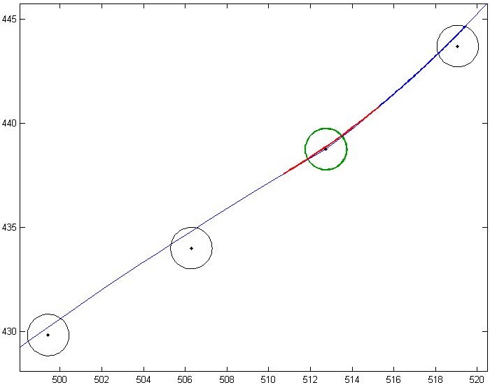
Figure 3: Example of good (on the left) and bad (on the right) junction points (green points). On the left the curve will have C0superscript๐ถ0C^{0} continuity. On the right, the red and blue curve is an example of smoothing biarc. Notice that the biarc is within the tolerance and that the final curve will be G1superscript๐บ1G^{1} continuous in the junction point.
Refer to caption
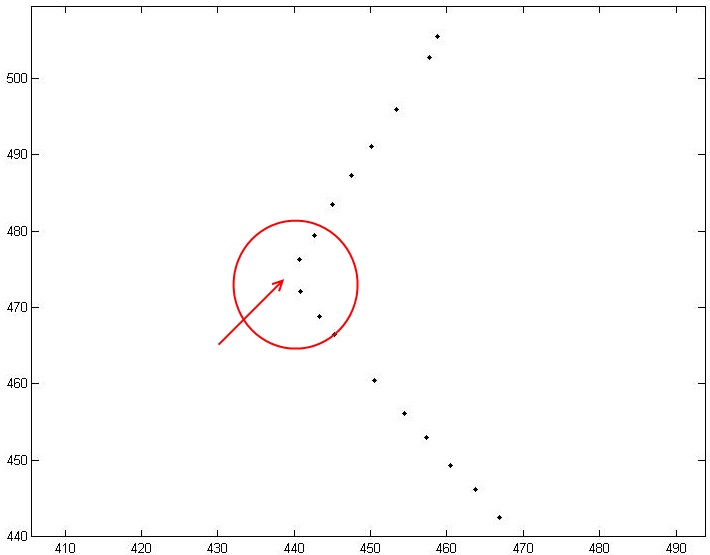
Figure 4: Example of smoothing arc in a neighbourhood of a bad point.

8 Regularity of the approximation

Before studying the regularity of the final curve, we need a brief summary. We start from a set of planar data points and we try to build all the possible arcs approximating any number of points (construction of matrix M๐‘€M). Then, we make a selection: we take in consideration only the longest arcs (construction of matrix G๐บG). Finally, if there are some points which havenโ€™t been approximated yet, we reapply all the previous steps in the missing sections, creating a continuous curve composed only by arcs or segments.

Clearly, itโ€™s quite difficult that all the section of the final curve join each other with C1superscript๐ถ1C^{1} continuity, because the approximation uses both arcs and segments. So the next problem we want to discuss is about how to smooth our junction points (j.p.). To do this we first need to recognize good j.p. from bad j.p. Let us fix a positive tolerance ฮต๐œ€\varepsilon and let ๐ksubscript๐๐‘˜\mathbf{P}_{k} be a junction point for some k๐‘˜k. Suppose that ๐ksubscript๐๐‘˜\mathbf{P}_{k} is the j.p. of two consecutive arcs Akโˆ’1subscript๐ด๐‘˜1A_{k-1}, Aksubscript๐ด๐‘˜A_{k} and let ๐“e,kโˆ’1subscript๐“๐‘’๐‘˜1\mathbf{T}_{e,k-1}, ๐“s,ksubscript๐“๐‘ ๐‘˜\mathbf{T}_{s,k} be respectively the final unit tangent vector of Akโˆ’1subscript๐ด๐‘˜1A_{k-1} and the initial unit tangent vector of Aksubscript๐ด๐‘˜A_{k}. We say that ๐ksubscript๐๐‘˜\mathbf{P}_{k} is a bad j.p. if

๐“s,kโ‹…๐“e,kโˆ’1=cosโกฯ‘<ฮต,โ‹…subscript๐“๐‘ ๐‘˜subscript๐“๐‘’๐‘˜1italic-ฯ‘๐œ€\mathbf{T}_{s,k}\cdot\mathbf{T}_{e,k-1}=\cos{\vartheta}<\varepsilon, (22)

where ฯ‘โˆˆ[0,ฯ€]italic-ฯ‘0๐œ‹\vartheta\in[0,\pi] is the angle between the two tangent vectors. For example, if ฮต=0.995๐œ€0.995\varepsilon=0.995, each angle greater than 6 degrees will be a bad angle. Each angle that doesnโ€™t satisfy (22) is called a good angle. Our task is to smooth out bad angles: we can only accept piecewise circular curves (PCC) whose junction points are good. This is a practical motivation: if the final object, whose profile is defined by our curve, has good junction points, itโ€™s easier to smooth out the entire contour, because the angles in good j.p. will be small enough. So if ๐ksubscript๐๐‘˜\mathbf{P}_{k} is a good j.p., we donโ€™t apply any changes to the PCC (see Figure 3 on the left). Otherwise, in order to increase the regularity of the curve in that particular point, we use biarcs. Indeed, as we have already explained, biarcs are G1superscript๐บ1G^{1} continuous, so they can regularize quite easily a C0superscript๐ถ0C^{0} continuous curve.

Suppose ๐ksubscript๐๐‘˜\mathbf{P}_{k} is a j.p. of two consecutive arcs Akโˆ’1subscript๐ด๐‘˜1A_{k-1}, Aksubscript๐ด๐‘˜A_{k} and let ฮด๐›ฟ\delta be a positive fixed tolerance. Then we can find two points ๐kโˆ’1subscript๐๐‘˜1\mathbf{Q}_{k-1}, ๐ksubscript๐๐‘˜\mathbf{Q}_{k} respectively on the arcs Akโˆ’1subscript๐ด๐‘˜1A_{k-1}, Aksubscript๐ด๐‘˜A_{k} satisfying โ€–๐kโˆ’1โˆ’๐kโ€–=โ€–๐kโˆ’๐kโ€–=ฮดnormsubscript๐๐‘˜1subscript๐๐‘˜normsubscript๐๐‘˜subscript๐๐‘˜๐›ฟ\|\mathbf{Q}_{k-1}-\mathbf{P}_{k}\|=\|\mathbf{Q}_{k}-\mathbf{P}_{k}\|=\delta, i.e. ๐kโˆ’1subscript๐๐‘˜1\mathbf{Q}_{k-1}, ๐ksubscript๐๐‘˜\mathbf{Q}_{k} are on the circumference with center ๐ksubscript๐๐‘˜\mathbf{P}_{k} and radius ฮด๐›ฟ\delta. The idea is to employ these two points as initial and final points of a biarc, starting from ๐kโˆ’1subscript๐๐‘˜1\mathbf{Q}_{k-1} and ending in ๐ksubscript๐๐‘˜\mathbf{Q}_{k} (see Figure 3 on the right). Moreover, we can easily compute the tangent vectors in ๐kโˆ’1subscript๐๐‘˜1\mathbf{Q}_{k-1} and ๐ksubscript๐๐‘˜\mathbf{Q}_{k} because we know the centers and the radius of Akโˆ’1subscript๐ด๐‘˜1A_{k-1}, Aksubscript๐ด๐‘˜A_{k} (a tangent vector of a circle is well-known). The biarc we build with this method regularize the PCC locally, in a neighbourhood of the j.p. ๐ksubscript๐๐‘˜\mathbf{P}_{k}.

Itโ€™s highly recommended to choose ฮด๐›ฟ\delta not too high nor too small. In the first case, we can obtain a biarc that doesnโ€™t satisfy the tolerance chosen at the beginning of the procedure โ€” remember that we are trying to build a PCC whose distance from the given points is less than a positive number we decide โ€”. In the second case we smooth out the curve with such a small radius that the approximating biarc would be very similar to our j.p., i.e. useless.

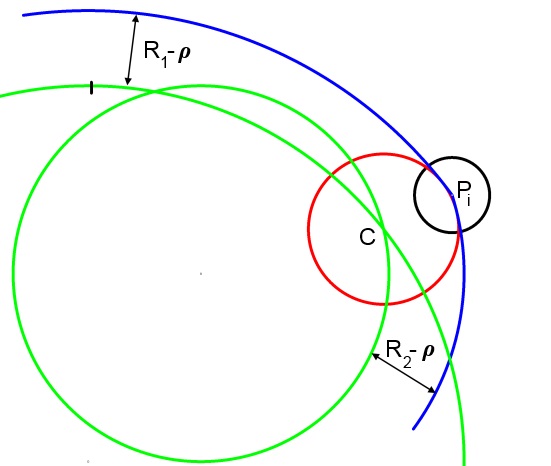
A second way to accomplish this task is to use simple arcs: given two arcs (possibly degenerate in segments) with a common j.p., itโ€™s always possible to build a simple arc approximating the j.p. within the tolerance and tangent to the other ones. If R1subscript๐‘…1R_{1}, R2subscript๐‘…2R_{2} are the radii of the two consecutive arcs, than we can increase or decrease them to obtain a new circle intersection whose distance from the two arcs is the same. This point will be the center of the tangent arc (see Figure 4).

9 Ensuring ๐‚๐ŸŽsuperscript๐‚0\mathbf{C^{0}} continuity and reducing the number of arcs

In the previous sections we discussed about how to find the longest arcs, how to fill the gaps among them and how to smooth the final curve. Now we want to describe a different method for approximating the data set, in order to build a C0superscript๐ถ0C^{0} continuous circular curve without any gap. This method tries to find a curve composed by a low number of arcs (not necessarily the minimum). This problem comes from a technical motivation: we want the CNC machine to perform a reduced number of movements. Clearly, minimizing the number of arcs means maximizing the number of approximated points for some arc. In this method we will use again the matrix M๐‘€M. The idea is quite simple but efficient. To fix ideas, suppose that Mโ€‹(1)=5๐‘€15M(1)=5. Then, we can build a least square arc starting from ๐1subscript๐1\mathbf{P}_{1}, ending in ๐5subscript๐5\mathbf{P}_{5} approximating ๐2,๐3,๐4subscript๐2subscript๐3subscript๐4\mathbf{P}_{2},\mathbf{P}_{3},\mathbf{P}_{4}. Suppose also that Mโ€‹(3)=3๐‘€33M(3)=3, Mโ€‹(4)=7๐‘€47M(4)=7, Mโ€‹(5)=4๐‘€54M(5)=4. Let A1subscript๐ด1A_{1} be the arc starting from ๐1subscript๐1\mathbf{P}_{1}, ending in ๐5subscript๐5\mathbf{P}_{5} and let A2subscript๐ด2A_{2} be the arc starting from ๐5subscript๐5\mathbf{P}_{5}, ending in ๐8subscript๐8\mathbf{P}_{8}. Then A1subscript๐ด1A_{1}, A2subscript๐ด2A_{2} will be C0superscript๐ถ0C^{0} continuous in ๐5subscript๐5\mathbf{P}_{5} and will approximate eight points in total. Now let A3subscript๐ด3A_{3} be the arc starting from ๐1subscript๐1\mathbf{P}_{1}, ending in ๐4subscript๐4\mathbf{P}_{4} and let A4subscript๐ด4A_{4} be the arc starting from ๐4subscript๐4\mathbf{P}_{4}, ending in ๐10subscript๐10\mathbf{P}_{10}. Then A3subscript๐ด3A_{3}, A4subscript๐ด4A_{4} will be C0superscript๐ถ0C^{0} continuous in ๐4subscript๐4\mathbf{P}_{4} and will approximate ten points in total. So A3subscript๐ด3A_{3}, A4subscript๐ด4A_{4} will be better than A1subscript๐ด1A_{1}, A2subscript๐ด2A_{2}, because they can approximate a higher number of points. Starting from the example we can develop the general case. Let S=Mโ€‹(i)๐‘†๐‘€๐‘–S=M(i), i=1,โ€ฆ,Nโˆ’2๐‘–1โ€ฆ๐‘2i=1,\dots,N-2, where N๐‘N is the number of points to be approximated. Then we can find a least square arc starting from ๐isubscript๐๐‘–\mathbf{P}_{i}, ending in ๐i+Sโˆ’1subscript๐๐‘–๐‘†1\mathbf{P}_{i+S-1}, and a least square arc starting from ๐i+Sโˆ’1subscript๐๐‘–๐‘†1\mathbf{P}_{i+S-1}, ending in ๐i+S+Mโ€‹(i+Sโˆ’1)โˆ’2subscript๐๐‘–๐‘†๐‘€๐‘–๐‘†12\mathbf{P}_{i+S+M(i+S-1)-2}. These two arcs will approximate S+Mโ€‹(i+Sโˆ’1)โˆ’1๐‘†๐‘€๐‘–๐‘†11S+M(i+S-1)-1 points in total. Now let j๐‘—j be an index such that i+2โ‰คjโ‰คi+Mโ€‹(i)โˆ’2๐‘–2๐‘—๐‘–๐‘€๐‘–2i+2\leq j\leq i+M(i)-2. We can build with the same technique two consecutive continuous arcs, the first one from ๐isubscript๐๐‘–\mathbf{P}_{i} to ๐jsubscript๐๐‘—\mathbf{P}_{j} and the second one from ๐jsubscript๐๐‘—\mathbf{P}_{j} to ๐j+Mโ€‹(j)โˆ’1subscript๐๐‘—๐‘€๐‘—1\mathbf{P}_{j+M(j)-1}, approximating jโˆ’i+1+Mโ€‹(j)โˆ’1=jโˆ’i+Mโ€‹(j)๐‘—๐‘–1๐‘€๐‘—1๐‘—๐‘–๐‘€๐‘—j-i+1+M(j)-1=j-i+M(j) points in total. So, if jโˆ’i+Mโ€‹(j)>S+Mโ€‹(i+Sโˆ’1)โˆ’1๐‘—๐‘–๐‘€๐‘—๐‘†๐‘€๐‘–๐‘†11j-i+M(j)>S+M(i+S-1)-1, these two arcs will be better than the first ones. Also here we will work with a new matrix G๐บG: at the beginning we set G=M๐บ๐‘€G=M; during the next steps, we will set Gโ€‹(j)=0๐บ๐‘—0G(j)=0 if Gโ€‹(j)๐บ๐‘—G(j) is not a starting point for some arcs (as we have already done in the previous sections).

  1. 1.

    Set i=1๐‘–1i=1, G=M๐บ๐‘€G=M;

  2. 2.

    While iโ‰คNโˆ’2๐‘–๐‘2i\leq N-2 do

  3. 3.

    Set S=Mโ€‹(i)๐‘†๐‘€๐‘–S=M(i), k=i๐‘˜๐‘–k=i, j=i+2๐‘—๐‘–2j=i+2;

  4. 4.

    Set Z=S+Mโ€‹(i+Sโˆ’1)โˆ’1๐‘๐‘†๐‘€๐‘–๐‘†11Z=S+M(i+S-1)-1;

  5. 5.

    While jโ‰คi+Mโ€‹(i)โˆ’2๐‘—๐‘–๐‘€๐‘–2j\leq i+M(i)-2 do

  6. 6.

    If jโˆ’i+Mโ€‹(j)>Z๐‘—๐‘–๐‘€๐‘—๐‘j-i+M(j)>Z

    k=j๐‘˜๐‘—k=j; Z=jโˆ’i+Mโ€‹(j)๐‘๐‘—๐‘–๐‘€๐‘—Z=j-i+M(j);

  7. 7.

    j=j+1๐‘—๐‘—1j=j+1;

  8. 8.

    For j=i+1,โ€ฆ,kโˆ’1๐‘—๐‘–1โ€ฆ๐‘˜1j=i+1,\dots,k-1

    Gโ€‹(j)=0๐บ๐‘—0G(j)=0;

  9. 9.

    For j=k+1,โ€ฆ,k+Wโ€‹(k)โˆ’2๐‘—๐‘˜1โ€ฆ๐‘˜๐‘Š๐‘˜2j=k+1,\dots,k+W(k)-2

    Gโ€‹(j)=0๐บ๐‘—0G(j)=0;

  10. 10.

    If iโ‰ k๐‘–๐‘˜i\neq k

    Gโ€‹(i)=kโˆ’i+1๐บ๐‘–๐‘˜๐‘–1G(i)=k-i+1;

  11. 11.

    i=k+Mโ€‹(k)โˆ’1๐‘–๐‘˜๐‘€๐‘˜1i=k+M(k)-1;

The matrix G๐บG determined in the algorithm is used then in the real approximation, and we can apply again the algorithm studied previously. As one can immediately notice, this method is better than the longest-arc-search algorithm if we take in consideration the regularity. Indeed, the final curve will be C0superscript๐ถ0C^{0} continuous. The worst case occurs when the final circular spline doesnโ€™t end precisely in the last point ๐Nsubscript๐๐‘\mathbf{P}_{N} but in ๐Nโˆ’1subscript๐๐‘1\mathbf{P}_{N-1}. In this situation we have to build a segment from ๐Nโˆ’1subscript๐๐‘1\mathbf{P}_{N-1} to ๐Nsubscript๐๐‘\mathbf{P}_{N} in order to achieve C0superscript๐ถ0C^{0} continuity.

10 Corner detection

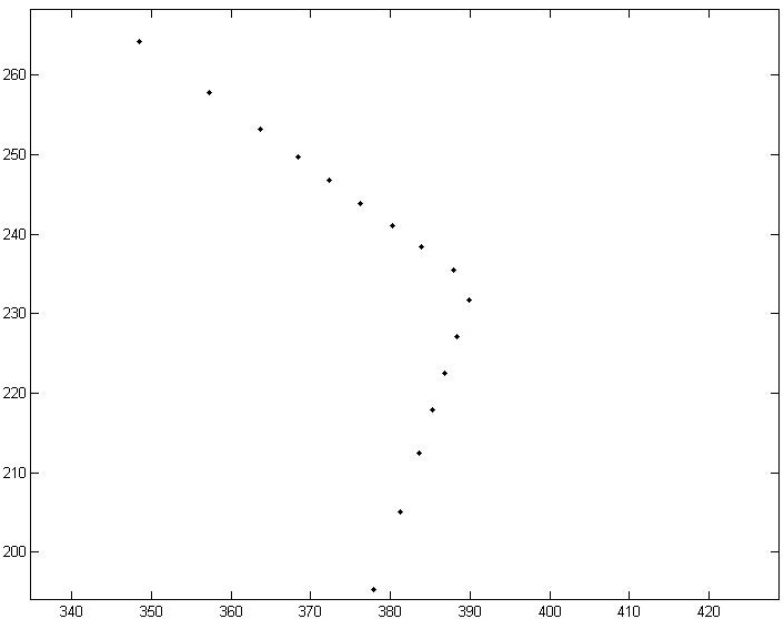
Up to now we have supposed that all the sections we want to approximate donโ€™t contain any corner points. In this paragraph we are going to explain how to detect corner points in the data set. This is not an easy problem, even when the points to be approximated are not affected by errors. We have to distinguish two different cases: the first one occurs when the data set actually contains corner points, i.e. there are some points that are also corners; the second one occurs when the corners are not in the data set, i.e. all the points are not corners. Itโ€™s easy to understand that the second case is more difficult and challenging than the first one. This case is caused by detection errors: several laser detectors canโ€™t give the exact position of corners. In presence of a corner, they create a sequence of points really close to it, but each of those points canโ€™t be considered as a good approximation of the corner. The first case can be solved with one of the algorithms explained in [1], [2], [6], [11], [12]. So, let us focus on the second case. The trivial idea is the following: suppose our data set is composed by N๐‘N distinct points ๐isubscript๐๐‘–\mathbf{P}_{i}; for each point we define two unit vectors

๐“1,i=๐iโˆ’1โˆ’๐iโ€–๐iโˆ’1โˆ’๐iโ€–,๐“2,i=๐i+1โˆ’๐iโ€–๐i+1โˆ’๐iโ€–,formulae-sequencesubscript๐“1๐‘–subscript๐๐‘–1subscript๐๐‘–normsubscript๐๐‘–1subscript๐๐‘–subscript๐“2๐‘–subscript๐๐‘–1subscript๐๐‘–normsubscript๐๐‘–1subscript๐๐‘–\begin{split}&\mathbf{T}_{1,i}=\frac{\mathbf{P}_{i-1}-\mathbf{P}_{i}}{\|\mathbf{P}_{i-1}-\mathbf{P}_{i}\|},\\ &\mathbf{T}_{2,i}=\frac{\mathbf{P}_{i+1}-\mathbf{P}_{i}}{\|\mathbf{P}_{i+1}-\mathbf{P}_{i}\|},\end{split}

and we compute the cosine of the angle ฮฑisubscript๐›ผ๐‘–\alpha_{i} between the two vectors, using the formula cosโกฮฑi=๐“1,iโ‹…๐“2,isubscript๐›ผ๐‘–โ‹…subscript๐“1๐‘–subscript๐“2๐‘–\cos{\alpha_{i}}=\mathbf{T}_{1,i}\cdot{\mathbf{T}_{2,i}}. Then, we say that ๐isubscript๐๐‘–\mathbf{P}_{i} is a corner if cosโกฮฑiโ‰ฅโˆ’ฮตsubscript๐›ผ๐‘–๐œ€\cos{\alpha_{i}}\geq-\varepsilon, where ฮต๐œ€\varepsilon is a positive value in [0,1)01[0,1). With few examples one can easily see that this condition is not sufficient to define corners, especially when the data set falls in the second case (when points are not corners). So we need another condition. The second requirement comes from a geometrical interpretation of curvature. We know that the curvature of a smooth curve at each point is the reciprocal of the radius of its osculating circle. If the curvature at the point x๐‘ฅx is a small number, then the curve will be similar to a line in x๐‘ฅx.

Refer to caption
Refer to caption
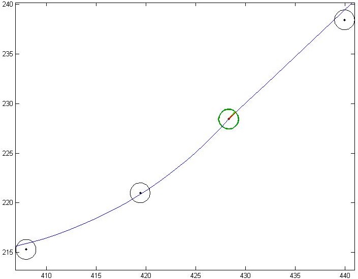
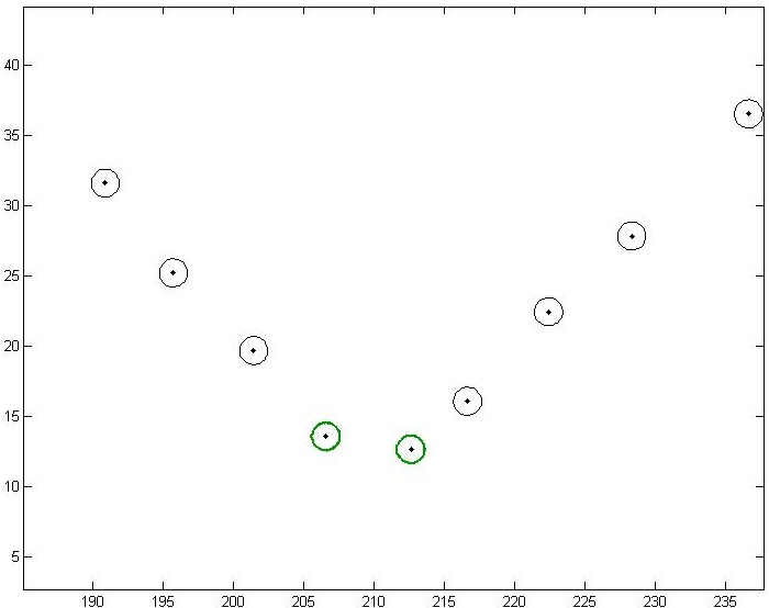
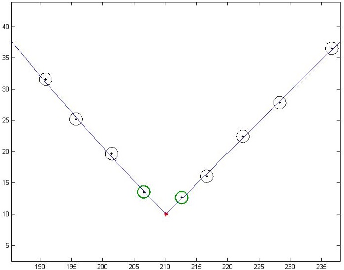
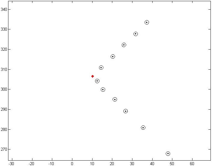
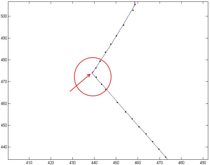
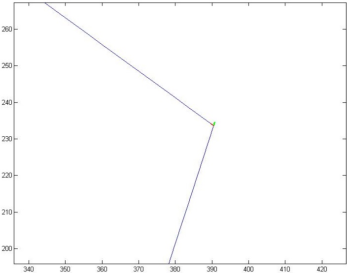
Figure 5: Example of undefined corner (on the left) and approximation of it (red point on the right). Here a tolerance of ฮด=1โ€‹mโ€‹m๐›ฟ1๐‘š๐‘š\delta=1\ mm was used. The green circles represent the anchor points detected by our algorithm using Rmโ€‹aโ€‹x=20โ€‹mโ€‹msubscript๐‘…๐‘š๐‘Ž๐‘ฅ20๐‘š๐‘šR_{max}=20\ mm and ฮต=0.98๐œ€0.98\varepsilon=0.98. The blue lines are least square contrained arcs.

Instead, if the curvature at x๐‘ฅx is high, then the curve will be similar to a small circle in x๐‘ฅx, i.e. the curve will quickly change direction. We will use the same principle to determine corner points.

Assume now that all the points of the data set have been captured by laser detector with constant step. Then, the distance from two consecutive points will be approximately the same. Let us choose two values ฮตโˆˆ[0,1)๐œ€01\varepsilon\in[0,1), Rmโ€‹aโ€‹x>0subscript๐‘…๐‘š๐‘Ž๐‘ฅ0R_{max}>0 and consider three consecutive points ๐iโˆ’1subscript๐๐‘–1\mathbf{P}_{i-1}, ๐isubscript๐๐‘–\mathbf{P}_{i}, ๐i+1subscript๐๐‘–1\mathbf{P}_{i+1} satisfying cosโกฮฑiโ‰ฅโˆ’ฮตsubscript๐›ผ๐‘–๐œ€\cos{\alpha_{i}}\geq-\varepsilon. Let R๐‘…R be the radius of the circle passing through those three points. We say that ๐isubscript๐๐‘–\mathbf{P}_{i} is an anchor point if R<Rmโ€‹aโ€‹x๐‘…subscript๐‘…๐‘š๐‘Ž๐‘ฅR<R_{max}.

Notice this: being an anchor point doesnโ€™t imply being a corner point. If ๐isubscript๐๐‘–\mathbf{P}_{i} is an anchor point, then itโ€™s quite probable that the actual corner point is in a neighbourhood of ๐isubscript๐๐‘–\mathbf{P}_{i}. In order to localize the corner we need two anchor points. Then, we compute ฮฑi+1subscript๐›ผ๐‘–1\alpha_{i+1}, ฮฑiโˆ’1subscript๐›ผ๐‘–1\alpha_{i-1} with the same technique described above. If cosโกฮฑi+1โ‰คcosโกฮฑiโˆ’1subscript๐›ผ๐‘–1subscript๐›ผ๐‘–1\cos{\alpha_{i+1}}\leq\cos{\alpha_{i-1}}, the two anchor points will be ๐isubscript๐๐‘–\mathbf{P}_{i} and ๐i+1subscript๐๐‘–1\mathbf{P}_{i+1}. Otherwise, they will be ๐isubscript๐๐‘–\mathbf{P}_{i} and ๐iโˆ’1subscript๐๐‘–1\mathbf{P}_{i-1}. Here one can understand the assumption that the distance from any two consecutive points is approximately the same: if the points are detected with adaptive steps techniques, itโ€™s hard to find a right value of Rmโ€‹aโ€‹xsubscript๐‘…๐‘š๐‘Ž๐‘ฅR_{max}.

After finding all the anchor points (two at a time), we use them to find corner points. Clearly, the corners need to be placed between these two points. The idea is to use another time the least square arcs. Suppose that ๐isubscript๐๐‘–\mathbf{P}_{i} and ๐i+1subscript๐๐‘–1\mathbf{P}_{i+1} are two consecutive anchor points. Let us consider the sets

ฮ›i,k={๐iโˆ’j:j=0,โ€ฆ,k},ฮ›i+1,h={๐i+j:j=1,โ€ฆ,h},formulae-sequencesubscriptฮ›๐‘–๐‘˜conditional-setsubscript๐๐‘–๐‘—๐‘—0โ€ฆ๐‘˜subscriptฮ›๐‘–1โ„Žconditional-setsubscript๐๐‘–๐‘—๐‘—1โ€ฆโ„Ž\begin{split}&\Lambda_{i,k}=\{\mathbf{P}_{i-j}:j=0,\dots,k\},\\ &\Lambda_{i+1,h}=\{\mathbf{P}_{i+j}:j=1,\dots,h\},\end{split}

where k,hโˆˆโ„•๐‘˜โ„Žโ„•k,\ h\in\mathds{N} and kโ‰ฅ2,hโ‰ฅ3formulae-sequence๐‘˜2โ„Ž3k\geq 2,\ h\geq 3. We want to increase k,h๐‘˜โ„Žk,\ h in order to build two arcs Ai,ksubscript๐ด๐‘–๐‘˜A_{i,k}, Ai+1,hsubscript๐ด๐‘–1โ„ŽA_{i+1,h} approximating respectively ฮ›i,ksubscriptฮ›๐‘–๐‘˜\Lambda_{i,k}, ฮ›i+1,hsubscriptฮ›๐‘–1โ„Ž\Lambda_{i+1,h} within a given positive tolerance ฮด๐›ฟ\delta. Notice this: the arcs we are building are not constrained arcs, i.e. they donโ€™t pass through any two given points. This time the best solution comes from Taubinโ€™s algorithm. For k=2,h=3formulae-sequence๐‘˜2โ„Ž3k=2,\ h=3, the solution is trivial because the circle passing through three distinct points always exists (degenerate in a line, eventually). So we try to increase k๐‘˜k and hโ„Žh (up to a maximum limit M๐‘€M) and we build Taubinโ€™s circles. If the distance between ฮ›i,ksubscriptฮ›๐‘–๐‘˜\Lambda_{i,k} and Ai,ksubscript๐ด๐‘–๐‘˜A_{i,k} is less than ฮด๐›ฟ\delta, k๐‘˜k need to be increased.

Otherwise, we decrease k๐‘˜k and, in this case, we build the three point circle. We do the same control for Ai+1,hsubscript๐ด๐‘–1โ„ŽA_{i+1,h}. At the end of the process, we will find two right values for k๐‘˜k and hโ„Žh and we will build the two corresponding arcs Ai,ksubscript๐ด๐‘–๐‘˜A_{i,k}, Ai+1,hsubscript๐ด๐‘–1โ„ŽA_{i+1,h}. These two arcs must intersect each other in two points. We select the nearest point to ๐isubscript๐๐‘–\mathbf{P}_{i}. This point will be the approximation of the corner point.

Pay attention to the fact that if the circles donโ€™t intersect each other, then there is something wrong in the data set or the algorithm detected two false anchor points. Another consideration: the corner points will be located approximately between the two anchor points because we used circles to find them: Taubinโ€™s method allows to create the best circle approximating a sequence of points, so itโ€™s reasonable to assume that Aisubscript๐ด๐‘–A_{i}, Ai+1subscript๐ด๐‘–1A_{i+1} are locally good approximations of the object contour.

  1. 1.

    Find two consecutive anchor points ๐isubscript๐๐‘–\mathbf{P}_{i}, ๐i+1subscript๐๐‘–1\mathbf{P}_{i+1};

  2. 2.

    Set k=3๐‘˜3k=3, h=4โ„Ž4h=4, fโ€‹lโ€‹aโ€‹gk=1๐‘“๐‘™๐‘Žsubscript๐‘”๐‘˜1flag_{k}=1, fโ€‹lโ€‹aโ€‹gh=1๐‘“๐‘™๐‘Žsubscript๐‘”โ„Ž1flag_{h}=1 , choose an integer Mโ‰ฅ4๐‘€4M\geq 4 and a tolerance ฮด>0๐›ฟ0\delta>0;

  3. 3.

    While k,hโ‰คM๐‘˜โ„Ž๐‘€k,\ h\leq M do

  4. 4.

    Find Taubinโ€™s circles Ai,ksubscript๐ด๐‘–๐‘˜A_{i,k}, Ai+1,hsubscript๐ด๐‘–1โ„ŽA_{i+1,h}

    approximating ฮ›i,ksubscriptฮ›๐‘–๐‘˜\Lambda_{i,k}, ฮ›i+1,hsubscriptฮ›๐‘–1โ„Ž\Lambda_{i+1,h};

  5. 5.

    If fโ€‹lโ€‹aโ€‹gk=1๐‘“๐‘™๐‘Žsubscript๐‘”๐‘˜1flag_{k}=1

  6. 6.

    If distโ€‹(Ai,k,ฮ›i,k)<ฮดdistsubscript๐ด๐‘–๐‘˜subscriptฮ›๐‘–๐‘˜๐›ฟ\text{dist}(A_{i,k},\Lambda_{i,k})<\delta

    k=k+1๐‘˜๐‘˜1k=k+1;

    else fโ€‹lโ€‹aโ€‹gk=0๐‘“๐‘™๐‘Žsubscript๐‘”๐‘˜0flag_{k}=0;

  7. 7.

    If fโ€‹lโ€‹aโ€‹gh=1๐‘“๐‘™๐‘Žsubscript๐‘”โ„Ž1flag_{h}=1

  8. 8.

    If distโ€‹(Ai+1,h,ฮ›i+1,h)<ฮดdistsubscript๐ด๐‘–1โ„Žsubscriptฮ›๐‘–1โ„Ž๐›ฟ\text{dist}(A_{i+1,h},\Lambda_{i+1,h})<\delta

    h=h+1โ„Žโ„Ž1h=h+1;

    else fโ€‹lโ€‹aโ€‹gh=0๐‘“๐‘™๐‘Žsubscript๐‘”โ„Ž0flag_{h}=0;

  9. 9.

    If fโ€‹lโ€‹aโ€‹gk=0๐‘“๐‘™๐‘Žsubscript๐‘”๐‘˜0flag_{k}=0 and fโ€‹lโ€‹aโ€‹gh=0๐‘“๐‘™๐‘Žsubscript๐‘”โ„Ž0flag_{h}=0

    return kโˆ’1๐‘˜1k-1, hโˆ’1โ„Ž1h-1; break;

  10. 10.

    Return kโˆ’1๐‘˜1k-1, hโˆ’1โ„Ž1h-1.

11 Testing the methods

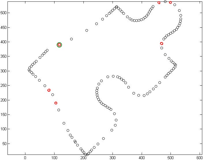
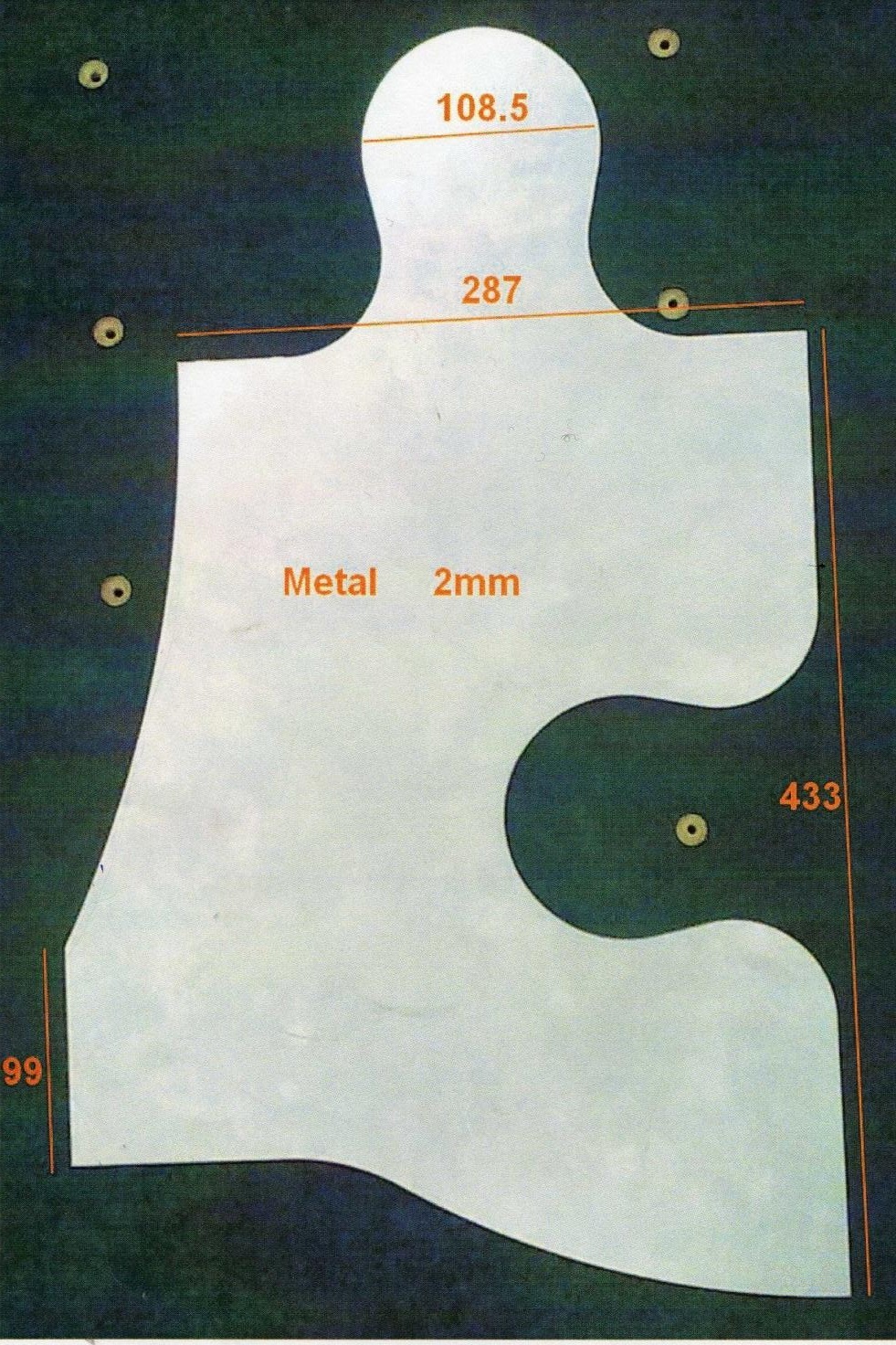
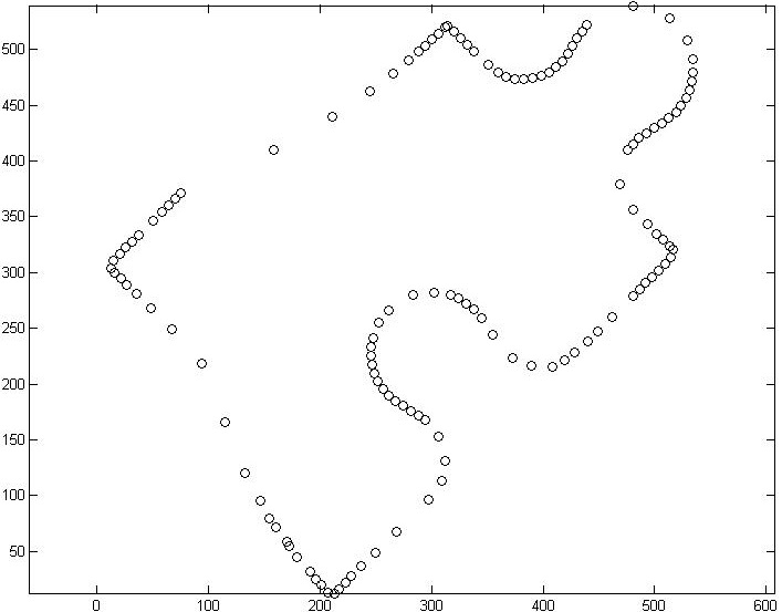
In this last section we want to give some examples of application of the two methods. First, we want to find a good approximation for the contour of the object represented in Figure 6 on the next page. We give a first rough approximation with 134 points captured by a laser detector (see Figure 6 again).
Refer to caption
Refer to caption
Figure 6: Metal 2D object to be approximated (on the left) and points captured by laser detector (on the right).
Refer to caption
Refer to caption
Figure 7: Improvement of the data set.
Refer to caption
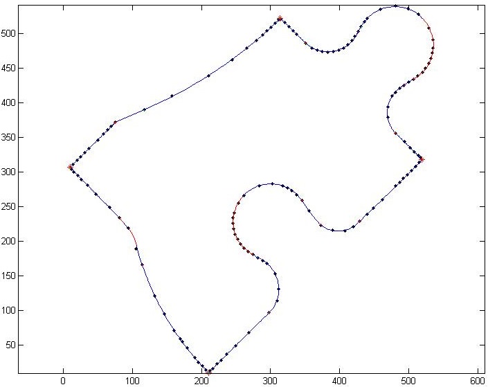
Figure 8: Approximation of the data set using longest arcs approach.

As one can see, this is a bad situation: the points are not uniform, i.e. they were determined with an adaptive method. We select this example because we want to show that the two methods also work in difficult cases. First, we try to improve the data set: since there are wide gaps between some points, we add six points (following a procedure that uses arc intersections) and we obtain the data set represented on Figure 7. Among the new points, the most important one is the green one, because the gap in that section of the contour is too wide to hope for a correct approximation. Secondly, we apply the detection algorithms and we find all five corner points. We use Rmโ€‹aโ€‹x=20โ€‹mโ€‹msubscript๐‘…๐‘š๐‘Ž๐‘ฅ20๐‘š๐‘šR_{max}=20mm, ฮต=0.9๐œ€0.9\varepsilon=0.9 (for detection of anchor points).

Table 1: Results with the first method.
Tolerance Arcs Segments Bad Points
1.5 mm 14 1 2
1 mm 17 3 6
0.5 mm 22 3 6
Table 2: Results with the second method.
Tolerance Arcs Segments Bad Points
1.5 mm 18 0 3
1 mm 21 1 2
0.5 mm 28 0 4

Notice this: adding the green points is crucial. Indeed, in this case the research of all the corner points fails, because the initial data set is ill-posed in a neighbourhood of one of the corners, i.e. there are not enough points to define a good approximation. Using the two methods, we find the results in Table222Here the tolerance is expressed in millimetres. Remember that 1 mm โ‰ˆ\approx 0.03937 Inches 1 and 2. As we expected, the number of arcs in the first method is less than the number of arcs in the second one. But using the second approach we create a continuous curve, so the number of segments is reduced.
Refer to caption
Refer to caption
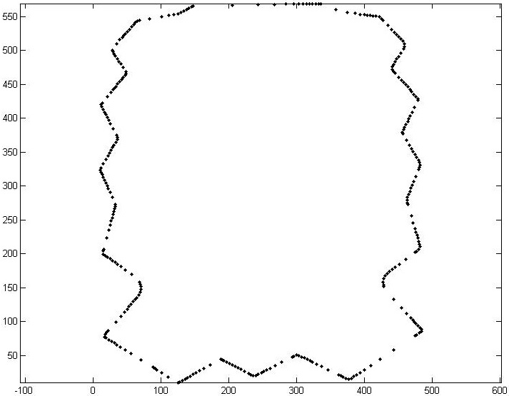
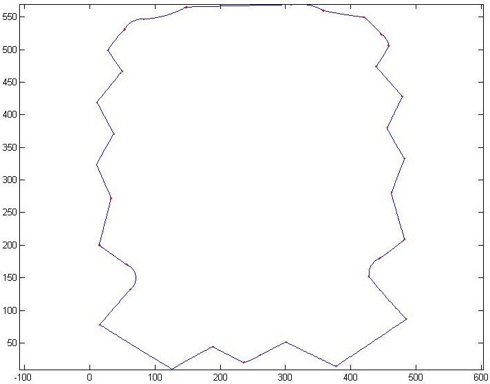
Figure 9: Contour of a wooden object (left) and approximation of it (right).
Refer to caption
Refer to caption
Figure 10: The true corners are not included in the data set.

Notice also that this method works better if the points are detected precisely. In our example, there are some detection errors, so it is better to use large error tolerance. If we try to use a tolerance smaller than 0.10.10.1, the final result is not reliable, because in the best case we would obtain a curve composed by arcs approximating a low number of points (three or four), so we would also have a high number of bad points.

Secondly, we want to approximate the contour of Figure 9. This time we donโ€™t need to build new points, because the sections between two consecutive corners are quite short and linear. However, we need to find a good approximation for corner points: as we can see in Figure 10 there is the same problem we faced in the other example, so the corner points are not included in the data set. Using Rmโ€‹aโ€‹x=20โ€‹mโ€‹msubscript๐‘…๐‘š๐‘Ž๐‘ฅ20๐‘š๐‘šR_{max}=20mm and ฮต=0.85๐œ€0.85\varepsilon=0.85 (for detection of anchor points) we find 18 corner points. After applying the second method, we have the results in Table 3.

Table 3: Results with the second method on the wooden object with ฮต=0.85๐œ€0.85\varepsilon=0.85.
Tolerance Arcs Segments Bad Points
1.5 mm 43 0 9
1 mm 46 0 10
0.5 mm 51 0 10
Table 4: Results with the second method on the wooden object with ฮต=0.9๐œ€0.9\varepsilon=0.9.
Tolerance Arcs Segments Bad Points
1.5 mm 38 0 4
1 mm 40 0 7
0.5 mm 43 0 7

We can notice that the number of bad points in Table 3 is quite high. This is justified by the fact that the algorithm detected only 18 corners, so at least three or four bad points should be corner points. Indeed, using ฮต=0.9๐œ€0.9\varepsilon=0.9 for detection of anchor points we find 21 corners and the results in Table 4.

Finally, we want to test the method in a simple case. The contour to be approximated is represented in Figure 11.
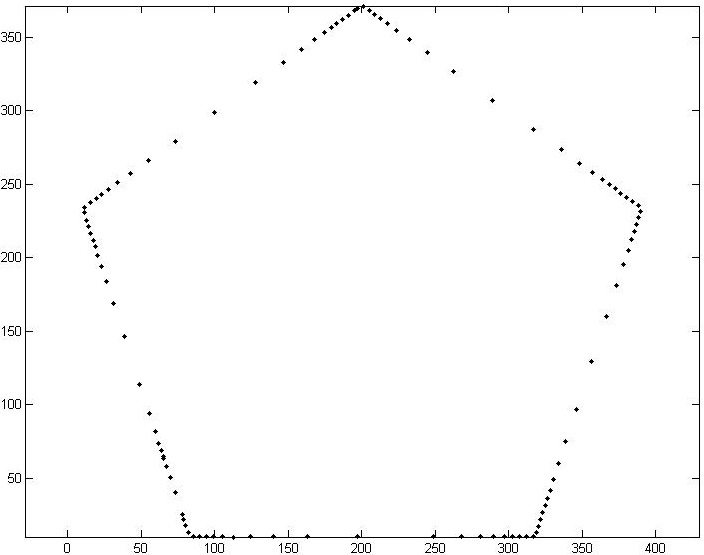
Refer to caption
Figure 11: Simple contour.

In this situation, the sections between two consecutive corners are simple lines, but there is still the problem of detecting the true corners, as we can notice in Figure 12. Using again Rmโ€‹aโ€‹x=20โ€‹mโ€‹msubscript๐‘…๐‘š๐‘Ž๐‘ฅ20๐‘š๐‘šR_{max}=20mm and ฮต=0.9๐œ€0.9\varepsilon=0.9 we find five corners and the results of Table 5.

Table 5: Results with the second method on the simple contour.
Tolerance Arcs Segments Bad Points
1.5 mm 5 0 0
1 mm 5 0 0
0.5 mm 5 0 0
Refer to caption
Refer to caption
Figure 12: Also in this case the corners are not included in the data set.

Conclusions

Two methods of approximation of a planar data set were presented. Both methods are based on arcs and segments. The first one searches the longest arcs in the data set and eventually fills the gaps among them using biarcs or segments. The second one creates a lower number of arcs but the final curve is more regular and C0superscript๐ถ0C^{0} continuous. Moreover, the number of segments is minimized. Finally, a method of corner detection was presented. The corners of the object contour are determined using circle intersections and Taubinโ€™s algorithm.

Aknowledgments

The author is very greatful to Professor C. Dagnino and Dr. D. Inaudi for their support and their suggestions.

References

  • [1] D. Chetverikov, A simple and efficient algorithm for detection of high curvature points in planar curves, Springer, Lecture notes in computer science, vol. 2756, 746-753, 2003
  • [2] H. Freeman, L. S. Davis, A corner-finding algorithm for chain-coded curves, IEEE Transactions on computers, 26:297-303, March 1977
  • [3] D. S. Meek, D. J. Walton, The family of biarcs that matches planar, two point G1superscript๐บ1G^{1} Hermite data, Elsevier, Journal of Computational and Applied Mathematics 212, 31-45, 2008
  • [4] C. J. Ong, Y. S. Wong, H. T. Loh, X. G. Hong, An optimization approach for biarc curve-fitting of B-spline curves, Elsevier, Computer-Aided Design, Vol. 28, 951-959, 1996
  • [5] H. Park, Error-bounded biarc approximation of planar curves, Elsevier, Computer-Aided Design, Vol. 36, 1241-1251, 2004
  • [6] G. V. Pedrosa, C. A. Z. Barcelos, Anisotropic diffusion for effective shape corner point detection, Elsevier, Patter Recognition Letters 31, 1658-1664, 2010
  • [7] L. A. Piegl, W. Tiller, Biarc approximation of NURBS curves, Elsevier, Computer-Aided Design, Vol. 34, 807-814, 2002
  • [8] L. A. Piegl, W. Tiller, Data approximation using biarcs, Springer-Verlag, Vol. 18, 59-65, 2002
  • [9] L. A. Piegl, W. Tiller, Least-Squares B-Spline Curve Approximation with Arbitrary End Derivatives, Springer-Verlag, Vol. 16, 109-116, 2000
  • [10] L. A. Piegl, W. Tiller, The NURBS book, Springer-Verlag, 1995
  • [11] A. Rosenfeld, E. Johnston, Angle detection on digital curves, IEEE Transactions on computers, 22:875-878, September 1973
  • [12] A. Rosenfeld, J. S. Weszka, An improved method of angle detection on digital curves, IEEE Transactions on computers, 24:940-941, September 1975
  • [13] J. R. Rossignac, A. A. G. Requicha, Piecewise-circular curves for geometric modeling, IBM J. Res. Develop., Vol. 31, 296-313, 1987
  • [14] X. Song, M. Aigner, F. Chen, B. Jรผttler, Circular spline fitting using an evolution process, Elsevier, Journal of Computational and Applied Mathematics 231, 423-433, 2008
  • [15] G. Taubin, Estimation of planar curves, surfaces, and nonplanar space curves defined by implicit equations with applications to edge and range image segmentation, IEEE Transactions on Patter Analysis and Machine Intelligence, Vol. 13, No. 11, November 1991
  • [16] Y. J. Tseng, Y. D. Chen, C. C. Liu, Numerically controlled machining of freeform curves using biarc approximation, Springer-Verlag, Vol. 17, 783-790, 2001