Attracting Lagrangian Coherent Structures on Riemannian manifolds
Abstract
It is a wide-spread convention to identify repelling Lagrangian Coherent Structures (LCSs) with ridges of the forward finite-time Lyapunov exponent (FTLE) field, and attracting LCSs with ridges of the backward FTLE. We show that in two-dimensional incompressible flows attracting LCSs appear as ridges of the forward FTLE field, too. This raises the issue of characterization of attracting LCSs from a forward finite-time Lyapunov analysis. To this end, we extend recent results by Haller & Sapsis (2011) Haller and Sapsis, 2011, regarding the relation between forward and backward maximal and minimal FTLEs, to both the whole finite-time Lyapunov spectrum and to stretch directions. This is accomplished by considering the singular value decomposition (SVD) of the linearized flow map. By virtue of geometrical insights from the SVD, we give a short and direct proof of the main result of Farazmand & Haller (2013) Farazmand and Haller, 2013, and prove a new characterization of attracting LCSs in forward time for Haller’s variational approach to hyperbolic LCSs Haller, 2011. We apply these results to the attracting FTLE ridge of the incompressible saddle flow.
Hyperbolic Lagrangian Coherent Structures (LCSs) are material surfaces that act as cores of mixing patterns in complex, unsteady and finite-time dynamical systems through material repulsion or attraction. In practice, repelling LCSs are often identified with ridges of the forward finite-time Lyapunov exponent (FTLE) field. Attracting LCSs are then defined as repelling LCSs in backward time. It is known that material structures experiencing strong shear induce large particle separation, and can hence appear as FTLE ridges as well. In the most frequently considered case of two-dimensional incompressible flows, we point out that also attracting LCSs are characterized by strong tangential particle separation, and may hence appear as forward FTLE ridges. We prove characterizations of attracting LCSs in forward time, which helps to determine the dynamical cause of particle separation.
I Introduction
In recent years, there has been an increasing interest in dynamical systems given on a finite time interval, driven by applications in geophysical fluid flows, biological models and engineering. Hyperbolic Lagrangian Coherent Structures (LCSs), i.e., codimension-one material surfaces with locally the strongest normal repulsion or attraction Haller and Yuan (2000), have been identified as the key structures governing transient pattern formation, transport and mixingPeacock and Haller (2013). As such, they are considered as finite-time analogues to stable and unstable manifolds of hyperbolic equilibria/trajectories in steady/unsteady flows admitting time-asymptotic solutions. Many approaches to numerical LCS detection have been developed, and most of them identify hyperbolic LCSs with ridges in scalar separation measure fields such as finite-time Lyapunov exponents (FTLEs)Haller (2001a); Shadden, Lekien, and Marsden (2005); Lekien, Shadden, and Marsden (2007), finite-size Lyapunov exponents (FSLEs)Joseph and Legras (2002), relative dispersionBowman (1999), and finite-time entropyFroyland and Padberg Gehle (2012).
A relation between hyperbolic LCSs and the FTLE field was first suggested by Haller Haller (2001a). The guiding intuition Haller (2001a, b) was that repelling LCSs should be indicated by curves (or surfaces) of (locally) maximal values—subsumed by an intuitive notion of ridges—of some separation measure, computed in forward time. In contrast, attracting LCSs were thought to be indicated by ridges obtained from a backward-time computation. This intuition has been adopted for the FTLE Shadden, Lekien, and Marsden (2005); Lekien, Shadden, and Marsden (2007), and is also present in the majority of approaches based on ridges of separation measures.
In this article, we show that in the two-dimensional incompressible case, strongly attracting structures necessarily induce strong particle separation and are hence indicated by forward FTLE ridges. This is in contradiction to the wide-spread hypothesis that any forward FTLE ridge corresponds to a repelling flow structure. There are several conceptual and computational issues related to that hypothesis Haller (2002); Branicki and Wiggins (2010); Haller (2011), including an example of an FTLE ridge induced by strong shear. To the best of our knowledge, the phenomenon of normally attracting forward FTLE ridges has been unknown and adds another aspect of mathematical inconsistency to purely ridge-based LCS approaches. After all, FTLE ridges may be induced by all sorts of dynamical phenomena, ranging from normal attraction via shear to normal repulsion.
Our example raises the question of how to determine attracting LCSs in a forward finite-time Lyapunov analysis. This question has been first considered in the context of the geodesic approach to hyperbolic LCSsFarazmand and Haller (2013). As we show in this work, one possible solution is to include principal directions in the LCS approach, as provided by the variational theory Haller (2011); Farazmand and Haller (2012a); Karrasch (2012) and the more recent geodesic theory of LCSs Haller and Beron-Vera (2012); Farazmand, Blazevski, and Haller (2014); Karrasch, Farazmand, and Haller .
In Section III, we extend recent results on the relation between forward and backward FTLEsHaller and Sapsis (2011) to both the whole finite-time Lyapunov spectrum and to associated principal directions. We develop the theory in the setting of Riemannian manifolds, which was first considered in Ref. Lekien and Ross, 2010 and is of interest in large-scale geophysical fluid flow applications. Our analysis strongly benefits from considering the singular value decomposition (SVD) of the deformation gradient tensor. Remarkably, even though the SVD is a well-established tool for the computation of Lyapunov spectra and Lyapunov vectors of time-asymptotic dynamical systems Greene and Kim (1987), its use in the finite-time context has been limited mostly to an alternative computation tool of the FTLE. Our analysis, however, also includes fields of subdominant singular values and singular vectors. This turns out to be of significant theoretical and computational advantageKarrasch, Farazmand, and Haller .
Section IV is devoted to the characterization of attracting LCSs in the geodesic Farazmand and Haller (2013); Blazevski and Haller (2014); Farazmand, Blazevski, and Haller (2014) and the variational Haller (2011) sense in forward time. In the first case, we provide a short and direct geometric proof of the main result of Ref. Farazmand and Haller, 2013. In the latter, the characterization is new and reveals that in two-dimensional incompressible flows, variational attracting LCSs satisfy ridge-type conditions for the forward FTLE field. We apply both approaches to the saddle flow discussed in Section II and show that both methods detect repelling and attracting LCSs correctly, irrespective of the orientation of a visual FTLE ridge.
II Example: A Nonlinear Incompressible Saddle
Consider dynamics around the autonomous, nonlinear, incompressible saddle, described by the HamiltonianKarrasch and Haller (2013)
Here, governs the strength of hyperbolicity, and localize the saddle behavior. Trajectories are given as solutions of the ordinary differential equation
We set the parameters to , and , and the resulting vector field on is shown in Fig. 1(a). Here, the origin is a hyperbolic steady state, with - and -axis as the classic stable and unstable manifolds, respectively. For any integration time, segments of the -axis centered around the origin are normally repelling, whereas similar segments of the -axis are normally attracting.
(a) 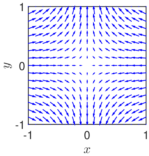
(b) 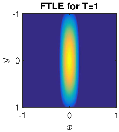
(c) 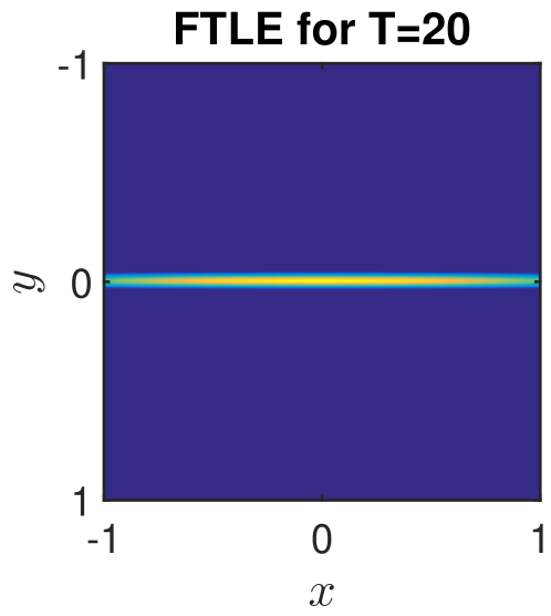
For (forward) integration time , we observe that the -axis appears visually as an FTLE ridge (Fig. 1(b)) and would be commonly misinterpreted as a repelling LCS on the time interval . This is in contradiction to its attracting nature. For a longer integration time of , the -axis appears visually as an FTLE ridge, while the -axis ridge seems to have disappeared, see Fig. 1(c).
For both integration times, however, segments of the respective complimentary axes can be shown to be FTLE height ridges Eberly et al. (1994). First, the directional derivatives of the FTLE field along the - and -axis in the respective normal direction vanish identically over the whole considered length. Second, the second-order directional derivatives are negative on and , respectively, see Fig. 2. Thus, locally around the origin, repelling and attracting material lines would be detected by a height ridge extraction algorithm, yielding a cross of ridges around the hyperbolic saddle. We will show later that segments of the normally atttracting -axis persist as an FTLE ridge for any integration time. As we demonstrated, for increasing integration time they shrink in length, eventually below grid resolution.
(a) 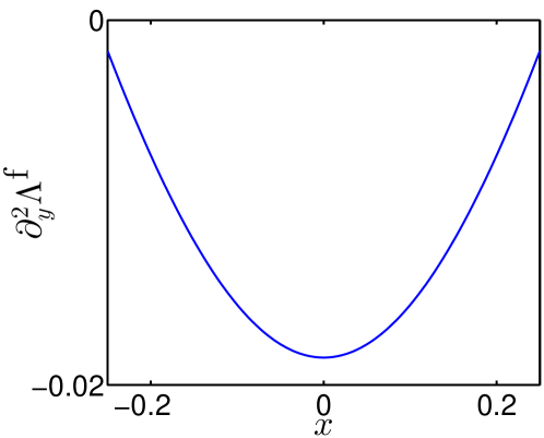
(b) 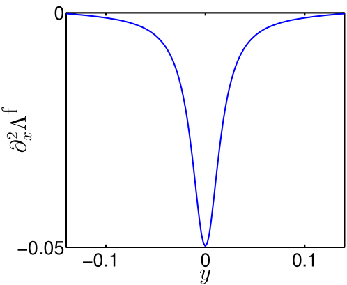
Based on this example, FTLE fields, which have been computed over a sufficiently long integration time, seem to indicate repelling or shearing material structures rather than attracting ones. In a flow with a priori unknown time scales or simply in a limited data set, however, it may be unclear whether the chosen/available integration time suffices to make the appearance of attracting LCSs as FTLE ridges unlikely. This in turn necessitates additional post-processing.
As indicated by this example and later theoretical results, defining attracting and repelling LCSs as FTLE ridges in backward and forward time, respectively, is mathematically inconsistent. This inconsistency does not restrict to the FTLE field as one representative of a separation measure. The reason is that separation measures do not indicate directions of stretching, but merely the pure fact of stretching. The orientation of a specified structure with respect to certain directions is defined only after its determination, and obviously cannot be obtained from the scalar field a priori. Additionally, in incompressible two-dimensional vector fields repulsion and attraction balance at each point, such that attracting structures come along with strong particle separation and may appear as ridges.
As we show in this work, one way to resolve this observed inconsistency is to consider directional information in LCS theory and computations.
III The Geometry of Linearized Deformation
In this section, we study finite-time flows on Riemannian manifolds. Thereby, we adopt the manifold framework of Ref. Lekien and Ross, 2010, where aspects related to the computation of the scalar FTLE field on non-Euclidean manifolds are discussed. We keep our presentation coordinate-free, and recall coordinate-representation issues in Appendix A.
Let be an -dimensional Riemannian manifold, i.e. a smooth manifold with a (Riemannian) metric. We denote the tangent space of at by . The metric gives rise to an inner product, and hence a norm, on each tangent space, and therefore induces a notion of angles between and length of tangent vectors.
Consider a nonautonomous velocity field on , defined on a finite time interval . The associated (particle) motion is then given by solutions of the ordinary differential equation
| (1) |
The -based flow map is denoted by and maps initial values from time to their position at time according to the unique solution of (1) passing through at time . Recall that the flow map is continuously differentiable in . In continuum mechanical terms, the flow map can be thought of as a one-parametric family of deformations of the flow domain Truesdell and Noll (2004).
Next, we consider the linearization of the flow map, also referred to as the deformation gradient (tensor) in continuum mechanics,
| or pointwise | ||||
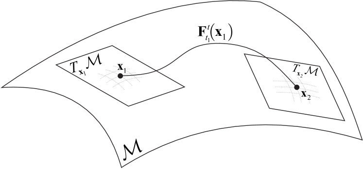
for , where the sub-index denotes push-forward Abraham, Marsden, and Ratiu (1988). Hence, the deformation-gradient tensor field is a vector bundle isomorphism over Abraham, Marsden, and Ratiu (1988), see Figs. 3 and 4 for illustrations.
In what follows, we study the dynamics from time to the final time , and abbreviate . In this setting, studying finite-time dynamics reduces to the (linearized) deformation analysis of a single iteration of a diffeomorphism.
Remark 1.
The fact that the deformation gradient is pointwise a mapping between two different vector spaces precludes formally to pose an eigenvalue problem for . When passing to a matrix representation of , the solution of the associated eigenvalue problem on depends on the choice of bases in the two tangent spaces with respect to which the matrix representation is computed. This phenomenon is also paraphrased as lack of objectivity/frame-invarianceMezic et al. (2010).
The linearized deformation effect of the flow map is best studied with the singular value decomposition (SVD) of , i.e.,
Here, and are pointwise orthogonal vector bundle homomorphisms, denotes the pointwise adjoint of with respect to the metric, and is a vector bundle isomorphism over . In orthonormal coordinates, and are represented by orthogonal matrices. The columns of , denoted by , are called right-singular vectors of , and the columns of , denoted by , are called left-singular vectors of . Right- and left-singular vectors form pointwise orthonormal bases of the corresponding tangent space. With respect to these bases, is represented pointwise by a diagonal matrix with positive entries , called the singular values of . In continuum mechanics, one also refers to them as stretch ratios (or principal stretches) and to the ’s and ’s as principal directions Truesdell and Noll (2004). Note, that we changed the order of indices compared to the usual SVD notation for consistency with literature related to finite-time Lyapunov analysis, see below.
It is worth recalling that the SVD is well-defined in the following sense, see, e.g., Ref. Trefethen and Bau, 1997, Thm. 4.1: requiring an ordering of the diagonal entries as above makes uniquely defined. Accordingly, an ordering of the normalized singular vectors is induced, which in turn are uniquely defined up to direction if the associated singular value is simple. Throughout this work, we assume the SVD of to be well-defined, and restrict, if necessary, our analysis to the open subset of the domain in which this holds true. This assumption guarantees the existence of two sets of (locally) smooth vector fields: the right-singular vector fields on , and the left-singular vector fields on . We choose to consider the scalar singular value fields to be defined on .
It is readily seen that right- and left-singular vectors are eigenvectors of right and left Cauchy–Green strain tensors, respectively, which are defined as
| (2) |
In contrast to , the right and left Cauchy–Green strain tensor fields are tangent bundle isomorphisms with base spaces and , respectively. Therefore, one can consider fiberwise eigenvalue problems, and Eq. (2) shows that right and left Cauchy–Green strain tensors, evaluated at and , respectively, have the same eigenvalues . They are related to the singular values of via .
The SVD can be reformulated in differential geometric notation as
| (3) |
One also says that and are -related, up to the non-vanishing, positive coefficient function . Eq. (3) states that the are mapped by onto and thereby stretched by , see Fig. 4.
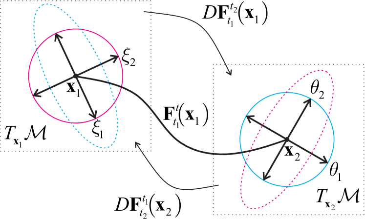
In words, and are the displacements around of, respectively, largest and smallest stretching under the linearized flow . At some point , the rate of largest stretching over the time interval of length is defined as
| (4) |
and is referred to as (forward) finite-time Lyapunov exponent (FTLE). If is incompressible, then the associated flow is volume-preserving, i.e., , and therefore ; see, e.g., Ref. Lee, 2012, Proposition 14.20, for the precise meaning of in the manifold framework. For two-dimensional incompressible flows we have in particular
| (5) |
Here and in the following, the superscript at singular value fields denotes the pointwise reciprocal.
Remark 2.
It is more common to introduce the FTLE and the principal directions via the eigendecomposition of than via the SVD of ; see Refs. Pobitzer et al., 2012; Ma and Bollt, 2014 for SVD-based approaches with a different focus. The SVD-approach has both theoretical and numerical advantages. First, is the natural object of study and its SVD gives the initial displacements of strongest and weakest stretching, together with their final displacements, see Fig. 4 and Remark 3 for another theoretical aspect. One numerical advantage is that the implementation of the SVD guarantees non-negative singular values and an orthogonal set of right- and left-singular vectors, in contrast to general eigendecomposition algorithms. Finally, SVD algorithms are less sensitive to perturbations than eigenvalue problem solversTrefethen and Bau (1997).
As mentioned in the Introduction, the flow map is also considered under backward integration, either from to , or from to . To keep our analysis related to the same time interval 111See also the discussion in Ref. Farazmand and Haller, 2013, we continue with our previous choice. The linearized deformation under the backward flow is then given by
| (6) |
where we have used by the chain rule and the orthogonality of and . Introducing backward singular value fields , defined on , we observe from Eq. (6) that the , obtained from the SVD of the forward , are exactly the backward principal directions. Furthermore, we have the relations
| (7) |
where denotes the pullback by Abraham, Marsden, and Ratiu (1988). Eqs. (7) relate all forward and backward principal stretches and directions to each other. Note the reversed ordering of -indices compared to the -indices, which is due to the fact that we keep the index order induced from the forward dynamics, see Fig. 4.
Remark 3.
In addition to the well-known advantages of SVD mentioned in Remark 2, another—seemingly overlooked—benefit from introducing deformation terms via the SVD of is that we obtain forward and backward stretch information from a single forward or backward time flow computation. This fact has been exploited recently for efficient and accurate LCS computations and trackingKarrasch, Farazmand, and Haller .
As a consequence, the backward FTLE is
| (8) |
which was first obtained in Ref. Haller and Sapsis, 2011, Prop. 1, and paraphrased there as: the largest backward FTLE equals the negative of the smallest forward FTLE . For two-dimensional incompressible flows, we re-derive Prop. 2 in Ref. Haller and Sapsis, 2011 from Eq. (5), i.e.,
| (9) |
Even though Eq. (9) has been derived earlierHaller and Sapsis (2011), a significant implication for visual FTLE ridge-based LCS approaches has been overlooked. For simplicity, suppose we identify a visual backward FTLE ridge at the final time, which is backward normally repelling. That is, is characterized by high -values relative to neighboring points off . Its flow-preimage at the initial time is a forward attracting LCS with high -values relative to neighboring points off , and thus appears as a visual forward FTLE ridge. Due to backward normal repulsion, is backward tangentially shrinking, and consequently may have a length on the scale of—or possibly below—computational resolution. Therefore, in practice the likeliness for a visually observable, attracting FTLE ridge depends on the ratio between the strength of hyperbolicity, the length of the FTLE ridge and the length of integration time. In any case, this does not affect the very fact that strongly forward attracting flow structures come along with high forward FTLE values, as demonstrated in Section II.
IV LCS Approaches Including Principal Directions
For most LCS approaches based on particle separation there are no explicit characterizations of attracting LCSs in forward time. In this section, we provide a short and direct proof of such a characterization for the geodesic approachFarazmand and Haller (2013), and the new corresponding result for the variational approachHaller (2011); Farazmand and Haller (2012b); Karrasch (2012). We revert the chronological order of the development of these two concepts, as the variational approach contains more mathematical conditions, covering those of the geodesic approach.
IV.1 Technical preliminaries
Definition 1 (Generalized maximum Eberly (1996)).
Let be a smooth scalar field, defined on some open subset , and be a smooth vector field on . Then is a generalized maximum of with respect to , if
Here, and denote, respectively, the first- and second-order Lie derivatives of with respect to at . A generalized minimum of is defined as a generalized maximum of .
The first- and second-order Lie derivatives correspond to directional derivatives. In the literature and the Euclidean case, they are also written as
Lemma 1.
Let and be smooth, normalized vector fields on some open subset and , respectively, and and be smooth scalar functions on and , respectively. Suppose the vector fields and the functions are -related, i.e. with a smooth, nowhere vanishing weight function , and or equivalently . Then the following equation holds for any and :
| (10) |
If (10) vanishes at , then
| (11) |
Proof.
IV.2 The relaxed variational/geodesic approach to hyperbolic LCSs
In the following, we will work with material surfaces, i.e., flow-invariant, time-parametric families of codimension-one submanifolds of , , satisfying for any .
Definition 2 (Strain- and stretch-surfaceFarazmand and Haller (2013)).
We call a material surface a forward strain- and stretch-surface if is everywhere normal to the right-singular vector fields and , respectively, i.e., for any one has, respectively,
| and |
We call a backward strain- and stretch-surface if is everywhere normal to the left-singular vector fields and , respectively, i.e., for any one has, respectively,
| and |
Strain-surfaces are normally repelling flow structures, while stretch-surfaces are normally attracting. Both types admit no Lagrangian shearHaller and Beron-Vera (2012). In dimension , strain- and stretch-surfaces are referred to as strain- and stretchlines. They have the local property, that they are pointwise aligned with the direction of strongest compression or stretching, respectively. In Ref. Farazmand, Blazevski, and Haller, 2014 it is shown that they also satisfy a global variational principle, and that they are null-geodesics of a Lorentzian metric. In dimension and higher, strain- and stretch-surfaces arise from a local variational principle, which compares candidate material surfaces to those perturbed in tangent orientation pointwise. Existence of (hyper-)surfaces orthogonal to a given (nonlinear) vector field as well as their numerical construction are challengingAbraham, Marsden, and Ratiu (1988); Palmerius, Cooper, and Ynnerman (2009), see Ref. Blazevski and Haller, 2014 for the local variational approach in dimension .
Theorem 1 (Farazmand and Haller, 2013, Theorem 1).
Forward strain-surfaces coincide with backward stretch-surfaces, and forward stretch-surfaces coincide with backward strain-surfaces.
Proof.
We prove only that backward strain-surfaces coincide with forward stretch-surfaces, the other statement can be shown analogously. The relation is equivalent to the fact that is the span of . is mapped bijectively to by by flow-invariance of . In turn, is spanned by and consequently orthogonal to . ∎
Example 1.
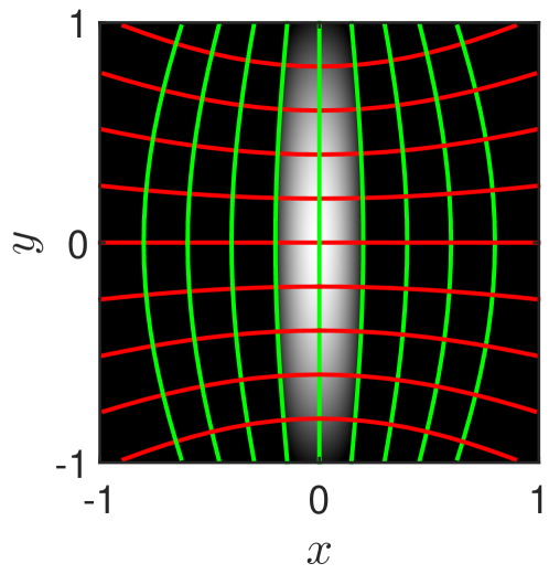
We apply the geodesic LCS approach to the saddle flow from Section II. Here, we only focus on checking the common hypothesis, that FTLE ridges computed in forward time correspond to repelling LCSs. in Fig. 5, we plot strainlines (red), which are normally repelling and do not pick up the visual FTLE ridge. In contrast, stretchlines, which are normally attracting, do align with the orientation of the visual ridge, which is picked up by the one passing through the saddle at the origin.
IV.3 The variational approach to hyperbolic LCSs
In Ref. Haller, 2011, hyperbolic LCSs are defined variationally as locally strongest normally repelling material lines. The local variational principle compares LCS candidate material surfaces to surfaces smoothly perturbed in position and tangent orientation.
Definition 3 (Variational hyperbolic LCSHaller (2011); Karrasch (2012)).
We call a compact material hypersurface a variational repelling LCS over if
-
1.
is a forward strain-surface, i.e. ,
-
2.
each is a generalized maximum of with respect to , i.e. and on , and
-
3.
at each one has .
We call a variational attracting LCS over if it is a variational repelling LCS over for the backward flow.
Note that the differentiability assumption on singular vector fieldsKarrasch (2012) is satisfied by our general hypothesis on simplicity of singular values. The third condition in Definition 3 requests that normal repulsion dominates tangential stretching.
Theorem 2 (Characterization of variational attracting LCSs).
Assume that is a variational attracting LCS over . Then the following statements hold:
-
1.
is a forward stretch-surface,
-
2.
each is a generalized minimum of with respect to , and
-
3.
at each one has .
Proof.
Corollary 1.
Let be a variational attracting LCS over for a two-dimensional incompressible velocity field. Then each satisfies in particular:
Corollary 1 states that variational attracting LCSs appear as curves of generalized maxima of the forward FTLE field, just as the variational repelling LCS. The distinction between these two types is via the direction field of differentiation. For attracting variational LCSs, the direction of largest stretching is tangential to the curve, as the direction of strongest attraction is normal to it. In contrast to the topological ridge approaches such as the height ridge, the variational approach, roughly speaking, selects ridges according to their orientation with respect to the directions of strongest attraction and repulsion, respectively.
Example 2.
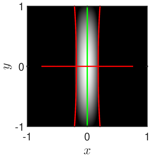
We apply the variational LCS approach to the saddle flow from Section II. In Fig. 6, we show curves of generalized maxima (red) of the forward FTLE w.r.t. (red) and w.r.t. (green). Irrespective of the orientation of the visual FTLE ridge, (parts of) the - and -axes are correctly detected as repelling and attracting LCSs, respectively. The vertical curves of generalized maxima of w.r.t. in Fig. 6 are discarded by checking for orthogonality with respect to (or, equivalently, for tangency with ). In general flows, this orthogonality requirement must be relaxed for numerical stabilityFarazmand and Haller (2012b).
V Conclusions
In this article, we showed that defining attracting and repelling LCSs as the ridges of scalar separation measure fields, computed in backward and forward time, respectively, is mathematically inconsistent. This adds to a collection of previously discovered issues in FTLE ridge-based LCS detection Haller (2002); Branicki and Wiggins (2010); Haller (2011); Norgard and Bremer (2012).
The reason for that inconsistency is the fact that separation measures reflect separation in an undirected fashion. The question, whether or not a certain structure of interest, such as a ridge, aligns with a certain direction field, can be answered only after the computation of the separation measure field and after the selection of the structure. In two-dimensional volume-preserving flows, the pointwise balance of particle separation and compression complicates the situation further. In this case, normally attracting material lines come along with large particle separation and may appear as ridges in separation measure fields.
This conceptual issue cannot be resolved by refinements in ridge notions, more accurate computations of separation measure fields, or improvements in numerical ridge extraction, but only by more involved LCS concepts. A natural extension of purely ridge-based LCS approaches is to incorporate principal directions in order to get a self-consistent notion of hyperbolic LCSs. In the recently developed geodesic approach Haller and Beron-Vera (2012); Farazmand and Haller (2012a); Blazevski and Haller (2014); Farazmand, Blazevski, and Haller (2014); Karrasch, Farazmand, and Haller , the principal direction fields are used to first define candidate structures. Only in a second step those structures are selected, which have the locally strongest intended dynamical impact. This way, normal repulsion and normal attraction are guaranteed from the beginning, while the second step guarantees the relevance for explaining finite-time pattern formation and transport.
Acknowledgements.
I would like to thank George Haller for support and helpful comments. Furthermore, I am grateful to Dan Blazevski, Florian Huhn, and especially Simon Eugster for fruitful discussions, to Joseph Lydon for proofreading the manuscript and to Mohammad Farazmand for sharing his strainline integration code. I am also thankful to Clancy Rowley for pointing out Ref. Trefethen and Bau, 1997.Appendix A Representation aspects in linearized deformation
In this section, we recall how to derive the metric representation of the deformation gradient, when is embedded in, say, Euclidean three-space, and the metric on is pulled back from that ambient space. As an example, we consider the two-dimensional sphere parametrized by geographical coordinates. Textbook references on the subject include Refs. Lee, 2012; Abraham, Marsden, and Ratiu, 1988, see also Ref. Lekien and Ross, 2010 for aspects on deformation gradient estimation on triangulated manifolds.
A.1 Preliminaries
Let be some -dimensional Euclidean vector space, and a basis. Then the matrix , , called the Gramian, is the metric representing matrix, which means the following.
Let and the unique representation of w.r.t. the basis . Then the -tuple is the coordinate representation of w.r.t. . Let with coordinate representations and . Then the inner product of and is given by
where the right-hand side is meant in terms of the usual matrix-multiplication. Note that the left-hand side is defined independently from any basis, but the right-hand side gives a recipe how to actually compute the inner product in coordinates.
The transformation given by the square root of yields a basis , , in which the inner product can be calculated in Euclidean fashion (recall that if a symmetric, (semi-)positive definite operator is given as , then the square root of is also referred to as the modulus of , and denoted by ). Indeed,
| (12) |
Because of Eq. (12), we refer to as the coordinate transformation to metric coordinates.
A.2 Pullback metrics
For convenience, we consider in the following exclusively , i.e., the Euclidean three-space with canonical inner product. We parametrize by the canonical embedding , and we refer to the three coordinate directions as . In these coordinates, the Riemannian metric is represented by
or, in other words, the metric representing matrix w.r.t. the canonical orthonormal dual basis is the identity matrix at each point.
Let be an embedded submanifold of , and assume for simplicity that (almost all of) can be described by a single parametrization , . Examples include the two-dimensional sphere of radius in geographical coordinates, i.e., longitude and latitude, and a three-dimensional spherical shell , . For definiteness, we consider only two-dimensional manifolds in the following.
With the parametrization , depending on parameters , and given in terms of -coordinates, the pushforward of vector fields in --coordinates by , is represented by
The pullback of differential forms by (in the dual --coordinates), as the dual mapping to the pushforward, is then represented by .
We turn into a Riemannian manifold, by pulling back the Euclidean metric by , i.e. . To compute in local coordinates, it suffices to compute the pullbacks of the canonical differential forms, for instance, . Their coordinates correspond to the respective column in the matrix representation of . A closer inspection of the emerging coefficients reveals that the metric representing matrix of can be computed formally as . Finally, the coordinate transformation to metric coordinates on the tangent space is given by .
A.3 Metric representations of deformation gradients
Let be the flow map as introduced in Section III. Consider the velocity field in Eq. (1) to be given in parameters, say, in longitude-latitude on the sphere, and to be computed in parameters as well. Then the Jacobian of in these coordinates is computed as
By the Courant–Fischer Min–Max TheoremAllaire and Kaber (2008), singular values and vectors of can be characterized as solutions of min-max-problems of
| (13) |
i.e., the deformation effect of at on a tangent vector . As usual, the norm of a tangent vector is given by . The question now is to which matrix representation to apply an svd-routine.
To this end, we transform the tangent vectors in Eq. (13) to metric coordinates, which yields:
| (14) |
where is the Euclidean norm of tuples. For the second identity, we substituted , or, equivalently, . Eq. (14) states that
is the metric representation of the deformation gradient. This can be used as input for an svd-routine. Finally, right- and left-singular vectors thus obtained need to be transformed to natural coordinates by and , respectively. After this step, they can be integrated to obtain strain- and stretchlines in the same parametrization as were given and initially.
A.4 Example
Consider the two-dimensional sphere of radius , , without the poles, with geographical parametrization given by
Then the pushforward of vector fields by (in --coordinates) is represented by
Thus, the metric representing matrix has the form
The diagonal form is a consequence of the orthogonality of the geographical parametrization, the deviation from the identity matrix is due to the lack of normalization. Clearly, the coordinate transformation to metric coordinates in the tangent space is then given by
| with inverse | ||||
Finally, the metric representation of the deformation gradient at , with coordinates , where , with coordinates , takes the form
| (15) |
References
- Haller and Sapsis (2011) G. Haller and T. Sapsis, “Lagrangian coherent structures and the smallest finite-time Lyapunov exponent,” Chaos 21, 023115 (2011).
- Farazmand and Haller (2013) M. Farazmand and G. Haller, “Attracting and repelling Lagrangian coherent structures from a single computation,” Chaos 23, 023101 (2013).
- Haller (2011) G. Haller, “A variational theory of hyperbolic Lagrangian Coherent Structures,” Physica D 240, 574–598 (2011).
- Haller and Yuan (2000) G. Haller and G. Yuan, “Lagrangian coherent structures and mixing in two-dimensional turbulence,” Physica D 147, 352–370 (2000).
- Peacock and Haller (2013) T. Peacock and G. Haller, “Lagrangian coherent structures: The hidden skeleton of fluid flows,” Physics Today 66, 41–47 (2013).
- Haller (2001a) G. Haller, “Distinguished material surfaces and coherent structures in three-dimensional fluid flows,” Physica D 149, 248–277 (2001a).
- Shadden, Lekien, and Marsden (2005) S. C. Shadden, F. Lekien, and J. E. Marsden, “Definition and properties of Lagrangian coherent structures from finite-time Lyapunov exponents in two-dimensional aperiodic flows,” Physica D 212, 271–304 (2005).
- Lekien, Shadden, and Marsden (2007) F. Lekien, S. C. Shadden, and J. E. Marsden, “Lagrangian coherent structures in n-dimensional systems,” J. Math. Phys. 48, 065404. 1–19 (2007).
- Joseph and Legras (2002) B. Joseph and B. Legras, “Relation between Kinematic Boundaries, Stirring, and Barriers for the Antarctic Polar Vortex,” J. Atmos. Sci. 59, 1198–1212 (2002).
- Bowman (1999) K. P. Bowman, “Manifold Geometry and Mixing in Observed Atmospheric Flows,” (1999), preprint.
- Froyland and Padberg Gehle (2012) G. Froyland and K. Padberg Gehle, “Finite-time entropy: A probabilistic approach for measuring nonlinear stretching,” Physica D 241, 1612–1628 (2012).
- Haller (2001b) G. Haller, “Lagrangian structures and the rate of strain in a partition of two-dimensional turbulence,” Physics of Fluids 13, 3365–3385 (2001b).
- Haller (2002) G. Haller, “Lagrangian coherent structures from approximate velocity data,” Physics of Fluids 14, 1851–1861 (2002).
- Branicki and Wiggins (2010) M. Branicki and S. Wiggins, “Finite-time Lagrangian transport analysis: stable and unstable manifolds of hyperbolic trajectories and finite-time Lyapunov exponents,” Nonlinear Processes in Geophysics 17, 1–36 (2010).
- Farazmand and Haller (2012a) M. Farazmand and G. Haller, “Computing Lagrangian coherent structures from their variational theory,” Chaos 22, 013128 (2012a).
- Karrasch (2012) D. Karrasch, “Comment on “A variational theory of hyperbolic Lagrangian Coherent Structures, Physica D 240 (2011) 574–598”,” Physica D 241, 1470–1473 (2012).
- Haller and Beron-Vera (2012) G. Haller and F. J. Beron-Vera, “Geodesic theory of transport barriers in two-dimensional flows,” Physica D 241, 1680–1702 (2012).
- Farazmand, Blazevski, and Haller (2014) M. Farazmand, D. Blazevski, and G. Haller, “Shearless transport barriers in unsteady two-dimensional flows and maps,” Physica D 278-279, 44–57 (2014).
- (19) D. Karrasch, M. Farazmand, and G. Haller, “Attraction-Based Computation of Hyperbolic Lagrangian Coherent Structures,” Journal of Computational Dynamics In press.
- Lekien and Ross (2010) F. Lekien and S. D. Ross, “The computation of finite-time Lyapunov exponents on unstructured meshes and for non-Euclidean manifolds,” Chaos 20, 017505 (2010).
- Greene and Kim (1987) J. M. Greene and J.-S. Kim, “The calculation of Lyapunov spectra,” Physica D 24, 213–225 (1987).
- Blazevski and Haller (2014) D. Blazevski and G. Haller, “Hyperbolic and elliptic transport barriers in three-dimensional unsteady flows,” Physica D 273-274, 46–62 (2014).
- Karrasch and Haller (2013) D. Karrasch and G. Haller, “Do Finite-Size Lyapunov Exponents Detect Coherent Structures?” Chaos 23, 043126– (2013).
- Eberly et al. (1994) D. Eberly, R. Gardner, B. Morse, S. Pizer, and C. Scharlach, “Ridges for image analysis,” J. Math. Imaging Vis. 4, 353–373 (1994).
- Truesdell and Noll (2004) C. Truesdell and W. Noll, The Non-Linear Field Theories of Mechanics, edited by S. S. Antman (Springer, 2004).
- Abraham, Marsden, and Ratiu (1988) R. Abraham, J. E. Marsden, and T. Ratiu, Manifolds, Tensor Analysis, and Applications, 2nd ed., Applied Mathematical Sciences, Vol. 75 (Springer, 1988).
- Mezic et al. (2010) I. Mezic, S. Loire, V. A. Fonoberov, and P. Hogan, “A New Mixing Diagnostic and Gulf Oil Spill Movement,” Science 330, 486–489 (2010).
- Trefethen and Bau (1997) L. N. Trefethen and D. Bau, Numerical linear algebra (SIAM, 1997).
- Lee (2012) J. M. Lee, Introduction to Smooth Manifolds, 2nd ed., Graduate Texts in Mathematics, Vol. 218 (Springer, 2012).
- Pobitzer et al. (2012) A. Pobitzer, R. Peikert, R. Fuchs, H. Theisel, and H. Hauser, “Filtering of FTLE for Visualizing Spatial Separation in Unsteady 3D Flow,” in Topological Methods in Data Analysis and Visualization II, Mathematics and Visualization, edited by R. Peikert, H. Hauser, H. Carr, and R. Fuchs (Springer, 2012) pp. 237–253.
- Ma and Bollt (2014) T. Ma and E. M. Bollt, “Differential Geometry Perspective of Shape Coherence and Curvature Evolution by Finite-Time Non-hyperbolic Splitting,” SIAM J. Appl. Dyn. Syst. 13, 1106–1136 (2014).
- Note (1) See also the discussion in Ref. \rev@citealpnumFarazmand2013.
- Farazmand and Haller (2012b) M. Farazmand and G. Haller, “Erratum and addendum to “A variational theory of hyperbolic Lagrangian coherent structures [Physica D 240 (2011) 574–598]”,” Physica D 241, 439–441 (2012b).
- Eberly (1996) D. Eberly, Ridges in Image and Data Analysis, Computational Imaging and Vision, Vol. 7 (Kluwer Academic Publishers, 1996).
- Palmerius, Cooper, and Ynnerman (2009) K. L. Palmerius, M. Cooper, and A. Ynnerman, “Flow field visualization using vector field perpendicular surfaces,” in Proceedings of the 25th Spring Conference on Computer Graphics, SCCG ’09 (ACM, 2009) pp. 27–34.
- Norgard and Bremer (2012) G. Norgard and P.-T. Bremer, “Second derivative ridges are straight lines and the implications for computing Lagrangian Coherent Structures,” Physica D 241, 1475 – 1476 (2012).
- Allaire and Kaber (2008) G. Allaire and S. M. Kaber, Numerical Linear Algebra, Texts in Applied Mathematics, Vol. 55 (Springer, 2008).