Dissecting galaxy formation models with Sensitivity Analysis – A new approach to constrain the Milky Way formation history

Abstract

We present an application of a statistical tool known as Sensitivity Analysis to characterize the relationship between input parameters and observational predictions of semi-analytic models of galaxy formation coupled to cosmological $N$-body simulations. We show how a sensitivity analysis can be performed on our chemo-dynamical model, ChemTreeN, to characterize and quantify its relationship between model input parameters and predicted observable properties. The result of this analysis provides the user with information about which parameters are most important and most likely to affect the prediction of a given observable. It can also be used to simplify models by identifying input parameters that have no effect on the outputs (i.e., observational predictions) of interest. Conversely, sensitivity analysis allows us to identify what model parameters can be most efficiently constrained by the given observational data set. We have applied this technique to real observational data sets associated with the Milky Way, such as the luminosity function of the dwarf satellites. The results from the sensitivity analysis are used to train specific model emulators of ChemTreeN, only involving the most relevant input parameters. This allowed us to efficiently explore the input parameter space. A statistical comparison of model outputs and real observables is used to obtain a “best-fitting” parameter set. We consider different Milky Way-like dark matter halos to account for the dependence of the best-fitting parameters selection process on the underlying merger history of the models. For all formation histories considered, running ChemTreeN with best-fitting parameters produced luminosity functions that tightly fit their observed counterpart. However, only one of the resulting stellar halo models was able to reproduce the observed stellar halo mass within 40 kpc of the Galactic center. On the basis of this analysis it is possible to disregard certain models, and their corresponding merger histories, as good representations of the underlying merger history of the Milky Way.

.

1. Introduction

The study of galaxy formation presents many theoretical challenges. A huge range of physical processes come into play, and often interact in nonlinear ways. Models of galaxy formation are rapidly growing in complexity to address both the physics we believe is required as well as the ever-expanding observational details (for a recent review, see Benson, 2010). A recent example of this observationally-driven model evolution came as a result of what is known as the “missing satellite problem” (Moore et al., 1999; Klypin et al., 1999). The overabundance of dark matter satellites in cosmological simulations with respect to the number of observed luminous satellites in, e.g., the Milky Way and M31 can be significantly alleviated thanks to the suppression of star formation in small halos that occurs during the epoch of re-ionization (Bullock et al., 2000; Gnedin, 2000). Current models of galaxy formation include phenomenological prescriptions to treat this process as one of their basic aspects. The luminosity-metallicity relation observed for Local Group dwarf galaxies is another example of complex physical processes that required the addition of new prescriptions to reproduce the available data sets (Dekel & Woo, 2003). Both model parameters and available observational constraints are growing at an extremely rapid pace.

Theoretical models include semi-analytic models such as ChemTreeN, Galform, or Galacticus (Tumlinson, 2010; Bower et al., 2010; Benson, 2012). These models use either extended Press-Schechter or N-body cosmological simulations to provide galaxy merger histories, and they apply prescriptions for the evolution of the baryonic components of the universe on top of this. Similarly, physics-rich cosmological simulations model the formation of galaxies in unprecedented detail, with a separate set of strengths and limitations. Both types of models are providing predictions about the distribution of observable quantities for galaxies – particularly Milky Way-type galaxies – in great detail. Recent examples include metallicity (Cooper et al., 2010; Font et al., 2011; Gómez et al., 2012a; Tissera et al., 2013b, a), stellar chemical abundances (Font et al., 2006), color profiles (Monachesi et al., 2013), luminosity and radial distributions of satellite galaxies (Koposov et al., 2008; Tollerud et al., 2008; Wang et al., 2013), and the degree of substructure in the phase-space of the stellar halo (Gómez et al., 2013).

Current and upcoming observational campaigns are providing tremendous amounts of data about the Milky Way and other galaxies. The Sloan Digital Sky Survey (SDSS), both through the photometric survey and the spectroscopic SEGUE project, has truly revolutionized our study of the Milky Way and its satellites, including finding many new ultra-faint dwarf galaxies (e.g. York et al., 2000; Belokurov et al., 2006, 2007; Bell et al., 2008; Yanny et al., 2009; Belokurov et al., 2010). SEGUE and the RAVE project (Steinmetz et al., 2006) have also provided velocity and metallicity information about huge numbers of stars, allowing new discoveries to be made (e.g. Carollo et al., 2008; Ivezić et al., 2008; Jurić et al., 2008; Carollo et al., 2010; Bond et al., 2010; Gómez et al., 2012b; Widrow et al., 2012; Siebert, 2012; Williams et al., 2013). The SDSS APOGEE project will extend our understanding of the chemical properties of the bulge, disk, and halo (Majewski et al., 2010), and the LAMOST spectroscopic project (Cui et al., 2012) will increase the number of halo stars found, supplementing the data taken by SEGUE and RAVE. In the future, the SkyMapper project (Keller et al., 2012), the Gaia satellite (Perryman et al., 2001), and their accompanying high-resolution spectroscopic follow-up campaigns (Barden et al., 2010; Gilmore et al., 2012) will produce even more detailed information about Milky Way stellar populations, providing a vastly larger and more uniform sample of high-resolution abundance measurements than currently exists (e.g., Frebel & Norris, 2013). In addition to the Milky Way and its satellites, detailed observations are being made of the stellar halos and satellite populations of other Milky Way-sized galaxies (e.g., Mouhcine et al., 2005; McConnachie et al., 2009; Radburn-Smith et al., 2011; Gilbert et al., 2012; Monachesi et al., 2013).

Taken together, recent and projected advances on all fronts in galaxy formation suggest that we are entering an era where robust statistical comparison between models and observations is essential. Several efforts are underway to develop the tools required for this enterprise (Henriques et al., 2009; Bower et al., 2010; Lu et al., 2012; Gómez et al., 2012a; Ruiz et al., 2013; Lu et al., 2013). In most of these works, the main goal was the identification of the “best” set of input parameters, or a region of best fit, within which a given set of observations could be successfully reproduced by a specific model. However, due to the growing complexity of the models and the non-linear coupling between physical processes therein, it is becoming increasingly important to incorporate statistical tools that allow one to identify and quantify the significance of relationships between input parameters and observable predictions. Sensitivity analysis is an example of this kind of statistical method, which provides a systematic and quantitative way of understanding the parameters that have the most influence in a given model and, in turn, could be most readily constrained with a given observational data set. It can also be used to simplify models by identifying input parameters that have minimal influence on the available set of outputs or observables.

In this work we demonstrate the use of sensitivity analysis in achieving the goals of both quantitatively and qualitatively understanding the relationships between input parameters and observable predictions for galaxy formation models – in particular, ChemTreeN, a semi-analytic model that has been used in several previous works (Tumlinson, 2006, 2010; Gómez et al., 2012a; Corlies et al., 2013). Such an analysis requires a very dense sampling of models within a high-dimensional space of input parameters. To make the project computationally feasible we supplement ChemTreeN with a statistical surrogate model known as a Gaussian process emulator. This tool can be used to give predictions for both model outputs and an attendant measure of uncertainty about these outputs at any point in the parameter space, and it is “trained” using a set of galaxy evolution models that span the required space (Bower et al., 2010; Gómez et al., 2012a, hereafter, G12). Through the combination of sensitivity analysis and Gaussian process model emulation, we can rapidly and reliably achieve our stated goals.

In addition to performing a sensitivity analysis, we apply our statistical machinery to an observational data set obtained from the Milky Way’s satellite dwarf galaxies. Guided by the results provided by the sensitivity analysis, we look for constraints on our model parameters from different observable quantities. As was previously shown by G12, we find that the best-fitting parameter values strongly depend on the merger history of the model being considered. Furthermore, we show how it is possible to constrain the formation history of the Milky Way by contrasting the best-fitting models to an independent set of observables.

This paper is structured as follows. Section 2 briefly describes the components of our galaxy evolution model, including the N-body simulations and the model itself. Section 3 describes the Gaussian process model emulator and our sensitivity analysis. Section 4 uses these models and statistical tools to understand the relationships between the input parameters and observable predictions made by the models, and Section 6 uses observations of the Milky Way dwarf galaxy population to show how these techniques could help us to constrain the Milky Way’s formation history as well as its properties at $z=0$. Finally, we discuss some of the limitations of this work and summarize our results in Section 7.

Throughout this study we work with both mock and real observational data sets. From now on we will refer to them as mock and real observables, respectively.

Table 1Main properties at $z=0$ of the four Dark Matter halos analyzed in this work.

Name	$R_{200}$	$M_{200}$	$c$	$z_{\rm LMM}$
$\text{MW}{1}$	381	1.63	12.2	2.1
$\text{MW}{2}$	378	1.59	9.2	3.5
$\text{MW}{3}$	347	1.23	15.5	2.0
$\text{MW}{4}$	366	1.44	13.6	3.0

Note. — From left to right, the columns give the simulation label, the virial radius of the dark matter halo, $R_{200}$, the mass within $R_{200}$, $M_{200}$, the concentration parameter, $c$, and the redshift of the last mayor merger, $z_{\rm LMM}$.

2. Numerical methods

Figure 1.— The different colored lines show the cumulative number of satellite galaxies as a function of absolute V-band magnitude, M_v, (left panel) and mean metallicity, $\langle$[Fe/H]$\rangle$, extracted from a set of 500 models used to train the model emulators. The black solid line shows the cumulative functions obtained from the fiducial model (see Table  2). The vertical black dashed lines indicate the values chosen to sample the respective cumulative functions.

In this Section we briefly describe the $N$-body simulations analyzed in this work, and also provide a brief summary of the main characteristics of our semi-analytical model ChemTreeN. For a detailed description of our numerical methods, we refer the reader to Tumlinson (2010), hereafter T10.

2.1. $N$-body simulations

Four separate simulations of the formation of Milky Way-like dark matter halos are analyzed in this work. The simulations were run using Gadget-2 (Springel, 2005) on a local computer cluster. Milky Way-like halos were first identified in a cosmological simulation with a particle resolution of $128^{3}$ within a periodic box of side 7.32 $h^{-1}$ Mpc. The WMAP3 cosmology (Spergel et al., 2007) was adopted, with matter density $\Omega_{m}=0.238$, baryon density $\Omega_{b}=0.0416$, vacuum energy density $\Omega_{\Lambda}=0.762$, power spectrum normalization $\sigma_{8}=0.761$, power spectrum slope $n_{s}=0.958$, and Hubble constant $H_{0}=73.2$ km s^-1 Mpc^-1. The candidates were selected to have gravitationally-bound dark matter halos with virial masses of M${}_{200}\approx 1.5\times 10^{12}$ M_⊙ at $z=0$ and no major mergers since $z=1.5$ - 2. These Milky Way-like dark matter halos were subsequently re-simulated at a resolution of $512^{3}$ by applying a multi-mass particle “zoom-in” technique. At this resolution, each dark matter particle in the highest-resolution region has a mass of $M_{p}=2.64\times 10^{5}$ M_⊙. Snapshots were generated at intervals of 20 Myr before $z=4$ and at 75 Myr intervals from $z=4$ to $z=0$. A six-dimensional friends-of-friends algorithm (Diemand et al., 2006) was applied to identify dark matter halos in each snapshot. The gravitational softening length was 100 comoving pc in all simulations. The main properties of the resulting dark matter halos are listed in Table  1.

Table 2Model Parameters.

Parameter	Fiducial Value	Range	Description	Explored
$z_{\rm r}$	10	5 – 19	Epoch of re-ionization	Yes
$f_{\rm bary}$	0.05	0 – 0.2	Baryonic mass fraction	Yes
$f_{\rm esc}$	50	0 – 110	Escape factor of metals	Yes
$\epsilon_{*}$	$1$	0.2 – 1.8	Star formation efficiency ($10^{-10}$ yr-1)	Yes
$m^{\rm II}_{\rm Fe}$	0.07	0.04 – 0.2	SN II iron yield ($M_{\odot}$)	Yes
$f_{\rm Ia}$	0.015	0.005 – 0.03	SN Ia probability	Yes
$\epsilon_{\rm SN}$	0.0015	0.0005 – 0.006	SNe energy coupling	Yes
$m^{\rm Ia}_{\rm Fe}$	0.5	$\cdots$	SN Ia iron yield ($M_{\odot}$)	No

2.2. Galactic chemical evolution model and particle tagging

In this work we use the semi-analytical model ChemTreeN, coupled to cosmological simulations, to follow the time evolution of the baryonic component of the stellar halos. In this context, a semi-analytic model consists of a set of coupled differential equations describing the evolution of baryons, including star formation and chemical enrichment, and derives its mass accretion histories and spatial information from the underlying N-body simulations. Processes such as star formation, stellar winds and chemical enrichment are introduced in the model through differential equations that are controlled via a set of adjustable input parameters. These parameters are commonly set to simultaneously match a range of observable quantities such as the galaxy luminosity functions (e.g. Bower et al., 2006) or a set of scaling relations (e.g. Kirby et al., 2011).

The general approach used in our models is to assume that each dark matter halo found in the simulations, and followed through the merger tree, possesses gas that has been accreted from the intergalactic medium (IGM), that this gas forms stars, that these stars return metals and energy to the host halo and to the larger environment, and that future generations of stars form with the now metal-enriched gas.

For every halo in the simulation, the star formation history is calculated using 10 timesteps between each redshift snapshot. At each timestep a star formation “parcel” is created with a single initial mass, metallically, and IMF. The metallicity for the parcel is derived from the present gas metallicity. Each parcel thus represents a single-age stellar population with a unique metallicity. When halos merge, their lists of parcels are concatenated. To explore the spatial, kinematic, and dynamical properties of stellar populations in the resulting halos “stars” are assigned to dark matter particles in the N-body simulation at each snapshot output. This is done by selecting a fraction of the most bound particles in each halo. The star formation that occurred between a given snapshot and the previous one is identified and an equal fraction of the newly formed stars is assigned to each of the selected particles. In this work only the $10\%$ most gravitationally bound particles in each halo are considered, in order to approximate the effect of stars forming deep in the potential well of the galaxy where dense gas would be most likely to collect.

What follows is a brief description of the physical prescriptions in ChemTreeN that are most relevant for this work. For more details about this model, we direct readers to our previous work (Tumlinson, 2006, 2010).

• Baryon Assignment

  The number of stars that a galaxy has formed throughout its history strongly depends on the amount of gas it contained. It is therefore important to define a prescription to model baryonic accretion into dark matter halos. Our models adopt a prescription based on that of Bullock & Johnston (2005) that heuristically takes into account the influence of a photoionizing background from the aggregate star formation in all galaxies. This model assigns a fixed mass fraction of baryons, $f_{\rm bary}$, to all dark matter halos before re-ionization, $z_{\rm r}$. After $z_{\rm r}$, gas accretion and therefore star formation are suppressed in small halos with a circular velocity below $v_{\rm c}=30$ km s^-1. Between $v_{\rm c}=30$ km s^-1 and 50 km s^-1, the assigned baryon fraction varies linearly from 0 to $f_{\rm bary}$. This baryon assignment is intended to capture the IGM “filtering mass” (Gnedin, 2000) below which halos are too small to retain baryons that have been heated to $T\gtrsim 10^{4}$ K by global re-ionization.

• Star Formation Efficiency

  Stars are formed with a constant efficiency, $\epsilon_{*}$, such that the mass formed into stars $M_{*}=\epsilon_{*}M_{\rm gas}\Delta t$ in time interval $\Delta t$. The star formation efficiency is equivalent to a timescale, $\epsilon_{*}=1/t_{*}$, on which baryons are converted into stars.

• Stellar Initial Mass Function

  An invariant stellar initial mass function (IMF) at all times and at all metallicities is assumed. The invariant IMF adopted is that of Kroupa (2001), $dn/dM\propto(m/M_{\odot})^{\alpha}$, with slope $\alpha=-2.3$ from $0.5$ – $140$ $M_{\odot}$ and slope $\alpha=-1.3$ from $0.1$ – $0.5$ $M_{\odot}$.

• Type Ia SNe

  Type Ia SNe are assumed to arise from thermonuclear explosions triggered by the collapse of a C/O white dwarf precursor that has slowly accreted mass from a binary companion until it exceeds the 1.4 $M_{\odot}$ Chandrasekhar limit. For stars that evolve into white dwarfs as binaries, the SN occurs after a time delay from formation that is roughly equal to the lifetime of the least massive companion. In our models, stars with initial mass $M=1.5-8$ $M_{\odot}$ are considered eligible to eventually yield a Type Ia SN. When stars in this mass range are formed, some fraction of them, $f_{Ia}$, are assigned status as a Type Ia and given a binary companion with mass obtained from a suitable probability distribution (Greggio & Renzini, 1983). The chemical evolution results are sensitive to the SN Ia probability normalization, $f_{Ia}$. The fiducial value of this parameter is fixed by normalizing to the observed relative rates of Type II and Type Ia SNe for spiral galaxies in the local universe (Tammann et al., 1994). This normalization gives a ratio of SN II to Ia of 6 to 1.

• Chemical Yields

  ChemTreeN tracks the time evolution of galaxies’ bulk metallicities by considering Fe as the proxy reference element. For Type Ia SNe with 1.5 – 8 $M_{\odot}$ the models adopt the W7 yields of Nomoto et al. (1997) for Fe, with 0.5 $M_{\odot}$ of Fe from each Type Ia SN. Type II SNe are assumed to arise from stars of 10 to 40 $M_{\odot}$, with mass yields provided by Tominaga (2009). They represent the bulk yields of core-collapse SNe with uniform explosion energy $E=10^{51}$ ergs. These models have $M=0.07$ – $0.15$ $M_{\odot}$ Fe per event.

• Chemical and Kinematic Feedback

  One possible cause of the observed luminosity-metallicity ($L$-$Z$) relation for Local Group dwarf galaxies is SN-driven mass loss from small dark matter halos (Dekel & Woo, 2003). To model this physical mechanism, ChemTreeN tracks mass loss due to SN-driven winds in terms of the number of SNe per timestep in a way that takes into account the intrinsic time variability in the star formation rate and rate of SNe from a stochastically sampled IMF. At each timestep, a mass of gas

  $$M_{\rm lost}=\epsilon_{\rm SN}\sum_{i}\dfrac{N^{i}_{\rm SN}E^{i}_{\rm SN}}{2v_{\rm circ}^{2}}$$ (1)

  becomes unbound and is removed permanently from the gas reservoir. Here $v_{\rm circ}$ is the maximum circular velocity of the halo, $N_{\rm SN}$ is the number of SNe occurring in a given timestep and $E_{\rm SN}$ is the energy released by those SNe. The only free parameter, $\epsilon_{\rm SN}$, expresses the fraction of the SN energy that is converted to kinetic energy retained by the wind as it escapes. The sum over index i sums over all massive stars formed in past timesteps that are just undergoing an explosion in the current timestep. Note that this approach allows for variations in the number and energy of SNe from timestep to timestep. The selective loss of metals that should arise when SNe drive their own ejecta out of the host galaxy is captured by the parameter $f_{\rm esc}$, which expresses the increased metallicity of the ejected winds with respect to the ambient interstellar medium. At each timestep, a total mass in iron $M^{\rm Fe}_{\rm lost}$ is removed from the gas reservoir of the halo:

  $$M^{\rm Fe}_{\rm lost}=f_{\rm esc}M_{\rm lost}\dfrac{M^{\rm Fe}_{\rm ISM}}{M_{\rm gas}}$$ (2)

  where $M^{\rm Fe}_{\rm ISM}$ is the total mass of iron in the ambient interstellar medium, $M_{\rm gas}\times 10^{\rm[Fe/H]}$ . This prescription ensures that, on average, the ejected winds are $f_{\rm esc}$ times more metal-enriched than the ambient interstellar medium. Alternatively, the fraction of metal mass lost from the halo is $f_{\rm esc}$ times higher than the total fraction of gas mass lost.

• Isochrones and Synthetic Stellar Populations

  To compare these model halos to observational data on the real Milky Way and its dwarf satellites, it is necessary to calculate the luminosities and colors of model stellar populations using pre-calculated isochrones and population synthesis models. Each star formation parcel possesses a metallicity, age, and a total initial mass distributed according to the assumed IMF. These three quantities together uniquely specify an isochrone and how it is populated. The models adopt the isochrones of Girardi et al. (2002, 2004) for the UBVRIJHK and SDSS ugriz systems, respectively, as published on the Padova group website. The lowest available metallicity in these isochrones is [Fe/H] = -2.3. Thus, this value is used to represent stellar populations with lower metallicities.

Table  2 summarizes the numerical values of the parameters used for our fiducial models, as well as the range of values over which they are allowed to vary.

3. Statistical Methods

In this Section we describe the statistical methods that are applied throughout the text. We start by reviewing the Gaussian process model emulation technique introduced in G12. We then describe in Section 3.2 a novel application of a technique known as Sensitivity Analysis which will allow us to characterize the input-output relationship of our chemo-dynamical model ChemTreeN.

3.1. Gaussian Process model emulator

In what follows we briefly describe how to train a Gaussian process model emulator (O’Hagan, 2006; Oakley & O’Hagan, 2002, 2004; Kennedy & O’Hagan, 2000) and we refer the reader to Gómez et al. (2012a) for a detailed description of the procedure (see also Bower et al., 2010). An emulator is constructed by conditioning a Gaussian process prior on a finite set of model outputs (or mock observables), collected at points dispersed throughout the parameter space. Once the emulator is trained it can rapidly give predictions of the model outputs, and an attendant measure of its uncertainty, at any point in the parameter space. In other words it acts as a statistical model of our much more computationally-expensive ChemTreeN model. Numerical implementations of Gaussian process emulators are computationally efficient, making it feasible to predict vast numbers of model outputs in a short period of time.

A Gaussian process is a stochastic process, all of whose finite-dimensional marginal distributions are multivariate normal – i.e., a single sample is normally distributed, a pair of samples have a two dimensional joint multivariate normal distribution, etc. Let $\mathcal{D}=\{\mathbf{x}_{1},\ldots,\mathbf{x}_{n}\}$ be a set of $n$ points in a $p$-dimensional input parameter space. We will refer to $\mathcal{D}$ as design. In this work a typical element of $\mathcal{D}$ is a 7-dimensional input parameter vector $\mathbf{x}=(z_{\rm r},~{}f_{\rm bary},~{}f_{\rm esc},~{}\epsilon_{*},~{}m^{\rm II}_{\rm Fe},~{}f_{\rm Ia},~{}\epsilon_{\rm SN},~{}m^{\rm Ia}_{\rm Fe})$. Let $\mathbf{Y}=\{y_{1},\ldots,y_{n}\}$ be the corresponding set of $n$ training values representing the model output at the design locations. For example, a typical element of $\mathbf{Y}$ is the cumulative number of Milky Way satellite galaxies at $M_{\rm v}\leq-5$, modeled by ChemTreeN at $\mathbf{x}\in\mathcal{D}$. The posterior distribution defining our emulator is

$$\mathcal{P}(\mathbf{Y}\mid\mathbf{x},\theta)\sim\mbox{GP}\left(m(\mathbf{x},\mathbf{\theta}),\Sigma(\mathbf{x},\mathbf{\theta})\right),$$

with

$$m(\mathbf{x}) =\mathbf{h}(\mathbf{x})^{T}\hat{\beta}+\mathbf{k}^{T}(\mathbf{x})\mathbf{C}^{-1}(\mathbf{Y}-{\bf H}\hat{\beta}),$$

$${\Sigma}(\mathbf{x}_{i},\mathbf{x}_{j}) =c(\mathbf{x}_{i},\mathbf{x}_{j})-\mathbf{k}^{T}(\mathbf{x}_{i})\mathbf{C}^{-1}\mathbf{k}(\mathbf{x}_{j})+\Gamma(x_{i},x_{j}),$$

$$\mathbf{C}_{ij} =c(\mathbf{x}_{i},\mathbf{x}_{j})$$ (3)

$$\Gamma(x_{i},x_{j}) =\left(\mathbf{h}(\mathbf{x_{i}})^{T}-\mathbf{k}^{T}(\mathbf{x_{i}})\mathbf{C}^{-1}{\bf H}\right)^{T}\left({\bf H}^{T}\mathbf{C}^{-1}{\bf H}\right)^{-1}$$

$$\left(\mathbf{h}(\mathbf{x_{j}})^{T}-\mathbf{k}^{T}(\mathbf{x_{j}})\mathbf{C}^{-1}{\bf H}\right),$$

$$\mathbf{k}(\mathbf{x})^{T} =\left(c(\mathbf{x}_{1},\mathbf{x}),\ldots,c(\mathbf{x}_{n},\mathbf{x})\right),.$$

Here, $m(\mathbf{x})$ is the posterior mean at $\mathbf{x}$, $\Sigma(\mathbf{x}_{i},\mathbf{x}_{j})$ is the posterior covariance between points $\mathbf{x}_{i}$ and $\mathbf{x}_{j}$, $\mathbf{C}$ is the $n\times n$ covariance matrix of the design $\mathcal{D}$, $\hat{\beta}$ are the maximum-likelihood estimated regression coefficients, $\mathbf{h}$ the basis of regression functions and ${\bf H}$ the matrix of these functions evaluated at the training points. The elements of the vector $\mathbf{k}(\mathbf{x})$ are the covariance of an output at $\mathbf{x}$ and each element of the training set.

To construct an emulator we need to fully specify our Gaussian process by choosing forms for the prior mean and covariance functions. We model the prior mean by linear regression with some basis of functions $\mathbf{h}(\mathbf{x})$. We use $\mathbf{h}(\mathbf{x})=\{1\}$ for simplicity. We specify a power exponential form for the covariance function,

$$c(\mathbf{x}_{i},\mathbf{x}_{j})=\theta_{0}\exp\left(-\frac{1}{2}\sum_{k=1}^{p}\left(\frac{|x_{i}^{k}-x_{j}^{k}|}{\theta^{k}}\right)^{\alpha}\right)+\delta_{ij}\theta_{N}.$$ (4)

Here $\theta_{0}$ is the marginal variance, the $\theta^{k}$ set characteristic length scales in each dimension in the parameter space and $\theta_{N}$ is a small term, usually called a nugget, added to ensure numerical convergence or to model some measurement error in the code output. The exponent $1\leq\alpha<2$ sets the roughness of the functions generated by the stochastic process. For this analysis we pick a value just less than $2$ which ensures smoothness. The shape of the covariance function sets how correlations between pairs of outputs vary as a function of the distances between the corresponding input vectors in the parameter space. The scales in the covariance function $\theta^{k}$ are estimated from the training data using maximum likelihood methods (Rasmussen & Williams, 2005).

A maximin Latin Hyper Cube (LHC) design is used to generate the training locations in the parameter space. This is an efficient design for space-filling in high dimensional parameter spaces. (Sacks et al., 1989; Santner et al., 2003). LHC sampling scatters $N$ points in a $p$-dimensional cube in such a way that all one and two-dimensional marginals have $N$ approximately uniformly-spaced points, while a regular grid would have only $N^{1/p}$ or $N^{2/p}$ distinct marginal points, respectively.

Following Gómez et al. (2012a) (see also B10), to compare the emulated model output to experimental data we define a univariate implausibility measure,

$$I^{2}(\mathbf{x})=\frac{({m}(\mathbf{x})-E[Y_{f}])^{2}}{{\Sigma}(\mathbf{x},\mathbf{x})+V[Y_{f}]},$$ (5)

where $Y_{f}$ represents the experimental or field data (real observables) that we seek to compare our model against, $E[Y_{f}]$ the expected value of $Y_{f}$ and $V[Y_{f}]$ the observational uncertainties. Large values of $I(\mathbf{x}_{t})$ indicate that the input parameter vector $\mathbf{x}_{t}$ is unlikely to give a good fit to the observable data. Note that $I(\mathbf{x})$ is a unit-less quantity.

The implausibility can be easily generalized to account for multivariate outputs. Consider a $t$-dimensional vector of model outputs $\mathbf{y(\mathbf{x})}=\{y_{1},\ldots,y_{t}\}$. Here, the elements of $\mathbf{y(\mathbf{x})}$ are, for example, the cumulative number of Milky Way satellite galaxies at $t$ different values of $M_{\rm v}$, modeled by ChemTreeN at $\mathbf{x}\in\mathcal{D}$. We extend our training set to be the $t\times n$ matrix $\mathbf{Y}=\{\mathbf{y(\mathbf{x}_{1})},\ldots,\mathbf{y(\mathbf{x}_{n})}\}$. We define the joint implausibility $J(\mathbf{x})$ for observables $\mathbf{Y_{f}}$ with measurement variance $V[\mathbf{Y_{f}}]$ and mean values $E[\mathbf{Y_{f}}]$:

$$J^{2}(\mathbf{x})=\left(E[\mathbf{Y_{f}}]-\mathbf{{m}}(\mathbf{x})\right)^{T}\\ \left(\mathbf{K}(\mathbf{x})+I\cdot V[\mathbf{Y_{f}}]\right)^{-1}\left(E[\mathbf{Y_{f}}]-\mathbf{{m}}(\mathbf{x})\right),$$ (6)

where $\mathbf{K}(\mathbf{x})$ represents the emulated $t\times t$ dimensional covariance matrix between the model outputs at the point $\mathbf{x}$ in the design space and $\mathbf{{m}}(\mathbf{x})$ is the $t$-dimensional emulator mean vector. This covariance-weighted combination of the multiple observables gives a reasonable indication of which input values $\mathbf{x}$ are predicted by the emulator to lead to model predictions close to the observed values $\mathbf{Y}$. Note that $J(\mathbf{x})$ is a $p$-dimensional scalar function, with $p$ the number of considered input parameters. For the optimal parameter vector $\mathbf{x}$, the quantity $J(\mathbf{x})^{2}$ has approximately a $\chi^{2}_{t}$ distribution (see discussion in G12), leading in the usual way to confidence sets in the input space. Following G12, we consider $75\%$ confidence sets.

Figure 2.— Main effects obtained from a seven-dimensional Gaussian process model emulator of ChemTreeN, where each dimension corresponds to a different input variable. The results were obtained using the simulation labeled MW1. The different panels show the results for different mock observables. From left to right, the columns correspond to eight different bins of the luminosity function. The corresponding mock observable is indicated on the top left corner of each panel. On each panel, the lines show the main effect associated with a different input variable, as indicated in the legend located at the bottom right corner. The range of each input variable has been normalized to the corresponding total extent, indicated in Table  2. From this figure it is possible to infer what parameters are most important to explaining the variability observed on each mock observable. Note as well that some parameters, such as $m_{\rm Fe}^{\rm II}$ and $f_{\rm Ia}$, do not show a strong influence on the values of the selected mock observables.

3.2. Sensitivity Analysis

Semi-analytical models are conceptually very simple. Individually, it may seem straightforward to forecast how variations of the input parameters associated with an adopted prescription can affect a given mock observable. However, the complex nonlinear couplings between different physical processes, in addition to the high dimensionality of the problem, can make this into an extremely challenging task. It is therefore desirable to implement techniques that allow one to statistically characterize the relationship between the input parameters and each mock observable. A sensitivity analysis is a very powerful technique for dissecting computer models (Smith et al., 2008), providing information about which parameters are the most important and most likely to affect the prediction of any given observable. It can also allow us to simplify our model by identifying input parameters that have little or no effect on the available set of outputs or mock observables. To carry out a sensitivity analysis (SA) on ChemTreeN, we follow the approach described by Schonlau & Welch (2006). Below we provide a short description of the method and we refer the reader to their work for more details.

The main goal of this analysis is to decompose the input-output relationship of ChemTreeN into a set of orthogonal quantities called main effects and interactions. These characterize how an output responds to variations of only a subset of input variables, allowing us to obtain a decomposition of the total variance observed. Main effects are those quantities in this expansion associated with variations of single input variables, and interactions or joint effects are those quantities associated with variations of two or more input variables.

Figure 3.— ANOVA decomposition (see 3.2) obtained from a seven dimensional Gaussian process model emulator of ChemTreeN, where each dimension corresponds to a different input variable. The results were obtained using the simulation labeled MW1. The different columns correspond to different mock observables, whereas rows are associated with either main effects or interactions. From left to right, the columns correspond to different bins of the luminosity function. We only consider up to two-variable interaction effects. Note that, for simplicity, not all interaction effects are shown. The different colors indicate the percentage of the total variance that can be explained by the corresponding effect. The total variance associated with each mock observable (column) has been normalized to one. This graphical representation of the ANOVA decomposition allows us to quickly identify what input parameters are more important in explaining the variability observed on each observable.

To apply a sensitivity analysis it is necessary to densely sample ChemTreeN over the whole range of interest of its input parameter space. With the ChemTreeN code, doing this rapidly becomes computationally prohibitive as the dimensionality of the input parameter space increases. Thus, we will perform a sensitivity analysis on the posterior mean associated with the corresponding Gaussian process model emulator, $\mathbf{m}(\mathbf{x},\mathbf{\theta})$. In what follows, for simplicity we will refer to the conditional mean as $m(\mathbf{x})$ and assume $t=1$, i.e., we will consider a single mock observable (see Section 3.1). Let us consider the effect of the subset of input variables $\mathbf{x}_{e}$, where $e$ denotes the indexes of the variables we are interested in. Note that $\dim(\{\mathbf{x}_{e},\mathbf{x}_{-e}\})=p$. The simplest approach to estimate the effect associated with $\mathbf{x}_{e}$ is to fix the remaining variables $\mathbf{x}_{-e}$ at a given value, e.g., their mid-ranges. However, the effect associated with the variables in $\mathbf{x}_{e}$ is likely to depend on the values chosen for $\mathbf{x}_{-e}$. Instead, effects are defined by averaging $m(\{\mathbf{x}_{e},\mathbf{x}_{-e}\})$ over $\mathbf{x}_{-e}$, ${\otimes_{\chi_{j}:~{}j\neq e}}$

$$\overline{m}_{\mathbf{x}_{e}}(\mathbf{x}_{e})=\int\limits_{\otimes_{\chi_{j}:~{}j~{}\neq~{}e}}m(\mathbf{x}_{e},\mathbf{x}_{-e})\,\prod_{j~{}\neq~{}e}\omega_{j}(x_{j})\,\mathrm{d}x_{j},$$ (7)

where $\omega_{j}(x_{j})$, with $j=1,\ldots,~{}p$, are a set of orthogonal weight functions, often chosen to be a uniform distributions, and

$$\chi=\otimes^{p}_{j=1}\,\chi_{j}$$ (8)

represent the domain of $m(\mathbf{x})$.

The effects defined in Equation 7 can be used to generate a decomposition of $m(\mathbf{x})$ into adjusted effects involving different numbers of input variables as follows:

$$\begin{split}m(\mathbf{x})=\mu_{0}+\sum_{j=1}^{p}\mu_{j}(x_{j})+\sum_{j=1}^{p-1}\sum_{j^{\prime}=j+1}^{p}\mu_{jj^{\prime}}(x_{j},x_{j^{\prime}})+\ldots+\\ \mu_{1,\ldots,p}(x_{1},\ldots,x_{p}),\end{split}$$ (9)

where

$$\mu_{0}=\int\limits_{\chi}m(\mathbf{x})~{}\omega(\mathbf{x})~{}\mathrm{d}\mathbf{x}$$ (10)

is an overall average,

$$\mu_{j}(x_{j})=\overline{m}_{j}(x_{j})-\mu_{0},~{}~{}{\rm for}~{}x_{j}\in\chi_{j}$$ (11)

is the adjusted main effect of $x_{j}$,

$$\begin{split}\mu_{jj^{\prime}}(x_{j},x_{j^{\prime}})=\overline{m}_{jj^{\prime}}(x_{j},x_{j^{\prime}})-\mu_{j}(x_{j})-\mu_{j^{\prime}}(x_{j^{\prime}})-\mu_{0},\\ {\rm for}~{}x_{j},x_{j^{\prime}}\in\chi_{j}\otimes\chi_{j^{\prime}},\end{split}$$ (12)

is the adjusted joint effect of $x_{j}$ and $x_{j^{\prime}}$ (often referred to as the first interaction), and so on. Note that each adjusted effect is just the corresponding effect corrected to remove all lower-order terms. An important property of the effects is that they are orthogonal with respect to the weight function, $\omega(\mathbf{x})$. This allows one to define a decomposition of the total variance of $m(\mathbf{x})$ as follows,

$$\begin{split}\int\limits_{\chi}[m(\mathbf{x})-\mu_{0}]^{2}~{}\omega(\mathbf{x})~{}{\rm d}\mathbf{x}=\sum_{j=1}^{p}\int\limits_{\chi_{j}}\mu_{j}^{2}(x_{j})~{}\omega_{j}~{}{\rm d}x_{j}+\\ \sum_{j=1}^{p-1}\sum_{j^{\prime}=j+1}^{p}~{}\int\limits_{\chi_{j}\otimes\chi_{j^{\prime}}}\mu_{jj^{\prime}}^{2}(x_{j},x_{j^{\prime}})~{}\omega_{j}(x_{j})~{}\omega_{j^{\prime}}(x_{j^{\prime}})~{}{\rm d}x_{j}~{}{\rm d}x_{j^{\prime}}+\ldots+\\ \int\limits_{\chi}\mu_{1,\ldots,p}^{2}(x_{1},\ldots,x_{p})\prod_{j=1}^{p}\omega_{j}(x_{j})~{}{\rm d}x_{j}.\end{split}$$ (13)

This ANalysis Of VAriance (ANOVA) decomposition offers a way to quantify the fraction of the total variance, shown on the left side of Eq. 13, that can be explained by variations of any single input variable or by a combination of two or more. Note that the larger the percentage, the more sensitive a mock observable is to the corresponding input variables.

Figure 4.— As in Figure 2, now for mock observables obtained from the cumulative number of satellite galaxies as a function of mean metallicity, $\langle$[Fe/H]$\rangle$.

Figure 5.— As in figure 3, for 4 bins of the cumulative number of satellite galaxies as a function of mean metallicity, $\langle$[Fe/H]$\rangle$.

4. Dissecting ChemTreeN – characterizing its input-output relationship

In what follows we will use the statistical tools described in the previous section to characterize in a quantitative way the relationships between input parameters and mock observable quantities produced by the ChemTreeN model. This is a useful exercise for several reasons. First, models of this sort are inexpensive compared to full-physics cosmological simulations, but take long enough to run (typically several hours) that sweeping through an entire range of parameter space is impractical, particularly if said parameter space has high dimensionality. As a result, models that produce a statistically good fit may only represent local maxima in probability, and thus other comparably good (or better) model parameter sets, and thus potentially interesting results, may be missed. Second, quantifying the relationships between input parameters (and combinations of parameters) and output values helps to highlight the most sensitive relationships between inputs and outputs, and to suggest areas where further experimentation with model prescriptions (possibly influenced by more physics-rich numerical simulations) would be particularly beneficial. Alternately, this allows us to find input parameters that have virtually no effect on the output values of interest, and which can be ignored in future experimentation. Third, performing such an analysis for the same ChemTreeN model using different N-body simulations helps both to identify universal commonalities and to find outputs where “implicit” parameters in the model (e.g., $z=0$ halo mass or merger history) are important.

In this section, we consider as mock observables the cumulative functions of the surviving satellites as a function of a) the absolute magnitude in the V-band and b) the satellite’s mean metallicity, $\langle[$Fe/H$]\rangle$. We will refer to them as the Luminosity Function (LF) and the Metallicity Function (MF), respectively. The advantage of using values of these cumulative functions as mock observables is that they are easy to emulate and, as we will show in what follows, they are most significantly influenced by a different set of input parameters. Once the relationship between these model outputs and input parameters has been established, we will turn our attention to a comparable set of real observables that have been extracted from a range of measurements of the Milky Way’s satellite galaxies.

Figure 6.— ANOVA decomposition obtained after coupling ChemTreeN with the dark matter-only N-body simulations MW1 (left) and MW2 (right). The same five dimensional design was used in both cases to create the training set. The different columns correspond to different mock observables, whereas rows are associated with either main effects or interactions. From left to right, the columns correspond to different bins of the luminosity function. Note that the ANOVA decomposition allows us to characterize the relationship between the input parameters and the desired model outputs, independently of the corresponding real observable values and the underlying formation history of our galactic model.

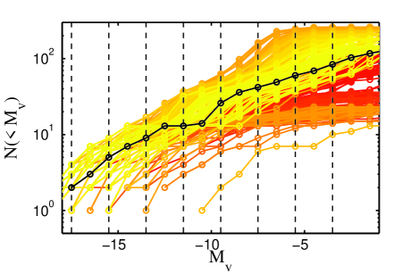
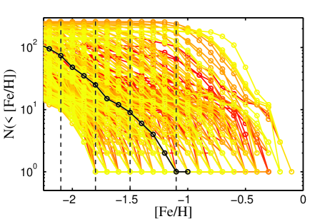
The first step in our analysis consists of constructing Gaussian process model emulators for the desired set of mock observables. The mock observables selected for emulation are values of the luminosity function and metallicity function at different locations of their respective domains. More precisely, we emulate the cumulative number of satellite galaxies above a range of values of M_v and $\langle$[Fe/H]$\rangle$. The respective values are indicated in Figure 1 with vertical black dashed lines. To train the emulators we created a training set consisting of $n=500$ models. These models were obtained after running ChemTreeN over 500 points dispersed throughout the input parameter space within the ranges specified in Table  2. This number of points was set to adequately balance the coverage of the input parameter space and the associated run time, and our results are insensitive to the number of training points (as long as a sufficient number are used). Each model of the training is computed after coupling ChemTreeN with the dark matter-only simulation MW1. We start by considering a seven-dimensional space of input parameters that includes the parameters flagged as “Yes” in Table  2. The resulting cumulative functions of all the training models are shown with different colors in Figure 1. As discussed in Section 3.1, a Gaussian process model emulator is a statistical model of ChemTreeN that allows us to obtain predictions of the desired model outputs, and an attendant measure of their uncertainty, at any point of the input parameter space. Once the model emulator is trained it is possible to compute the main effects and first interactions (joint influence of two parameters) as described in Section 3.2.

We train two different sets of model emulators. This is done by using outputs extracted either solely from the luminosity function or from the metallicity function. In Figure 2 we show the main effects computed for mock observables extracted from the luminosity function. Each panel corresponds to a different bin in the luminosity function, from most luminous (top left) to least luminous (bottom right). Each line is associated with a separate input parameter, as shown in the key. Each line tells us how the number of satellite galaxies at a given value of M_v varies as we vary a single input parameter of ChemTreeN, averaging the model emulator over the remaining six-dimensional input parameter space. For the purposes of comparison, the range within which each parameter is allowed to vary has been normalized from $0-1$. From the top left panel we can observe that, as expected, the number of satellite galaxies in the bright end of the luminosity function mainly depends on the value assigned to the baryon fraction, $f_{\rm bary}$. For this particular cosmological simulation, the cumulative number of satellites at M${}_{\rm v}=-17.5$ could take any value between 0 and $\sim 6$ simply by varying the value of this parameter within the range permitted by the emulator. We can also immediately see a much weaker dependence on the star formation efficiency, $\epsilon_{*}$. Note that the remaining parameters have almost no effect on this particular mock observable. As we move toward the faint end of the luminosity function (i.e., less negative values of M_v), the parameter $f_{\rm bary}$ becomes less important and the redshift of the epoch of reionization, $z_{\rm r}$, starts to take over. At M${}_{\rm v}=-3.5$, in the regime of the ultra faint dwarf galaxies, the number of satellite galaxies is strongly dominated by $z_{\rm r}$, with a much weaker dependence on $f_{\rm bary}$. Again, we find that variation of the remaining parameters does not significantly affect the cumulative number of galaxies in this magnitude bin.

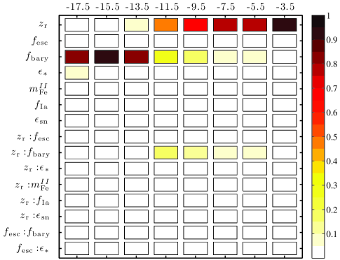
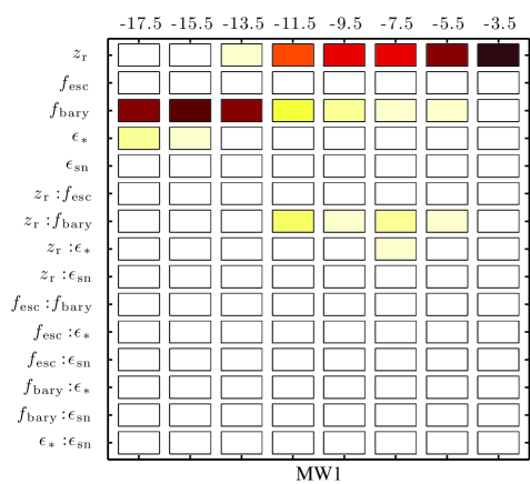
Figure 3 shows the relative magnitude of each of the seven main effects and the eight most important two-way interaction effects (as rows), for each luminosity bin level (as columns). The first column, for example, shows that over $95\%$ of the variance in the number of mock bright satellite galaxies in the V-band magnitude M${}_{\rm v}=17.5$ is accounted for by variation in the baryon fraction $f_{\rm bary}$, with most of the remainder accounted for by variations in star formation efficiency $\epsilon_{*}$. It is interesting to observe how, as we move toward fainter magnitudes, the fraction of variance explained by variations of $f_{\rm bary}$ decreases whereas the one associated with $z_{\rm r}$ increases. The transition takes place at around M${}_{\rm v}\approx-11.5$. At this M_v, the interaction effect $z_{\rm r}~{}:~{}f_{\rm bary}$ becomes important, indicating a coupling of both input parameters. This coupling can be clearly observed on the top right panel of Figure 2.

From Figure 3 we can infer that observables extracted from the luminosity function could only be used to constrain parameters such as $f_{\rm bary}$, $z_{\rm r}$ and, to a much lesser extent, $\epsilon_{*}$. In our models, the remaining four parameters cannot account for significant variations of the cumulative number of galaxies at any magnitude bin – or, taken another way, the observables we have chosen provide no meaningful constraints on these particular parameters. Thus, a different set of observables is required if we wish to constrain any of the remaining model parameters.

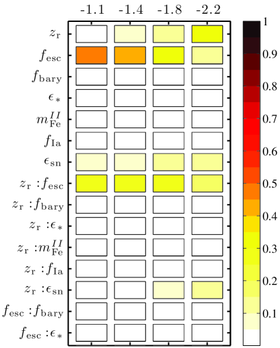
In Figure 4 we show the main effects computed for mock observables extracted from the metallicity function. The first panel shows that the cumulative number of satellite galaxies with $\langle$[Fe/H]$\rangle\geq-1.1$ strongly depends on the escape factor of metals, $f_{\rm esc}$. There is also a much weaker dependence on the value assigned to the supernova energy coupling, $\epsilon_{\rm SN}$, and to the redshift of reionization, $z_{\rm r}$. In a similar fashion to what was observed for the luminosity function observables, as we move toward lower values of $\langle$[Fe/H]$\rangle$ the number of satellite galaxies rapidly increases and $z_{\rm r}$ becomes the dominant parameter. Figure 5 shows the corresponding ANOVA decomposition. We can clearly observe how the variance on the cumulative number of metal-rich satellite galaxies (defined here to be $\langle$[Fe/H]$\rangle\geq-1.1$) is closely associated with variations of $f_{\rm esc}$ and only slightly on $\epsilon_{\rm sn}$, whereas the cumulative number of satellites with $\langle$[Fe/H]$\rangle\geq-2.2$ is dominated by the parameter $z_{\rm r}$. The remaining parameters have a negligible effect on the cumulative number of galaxies as a function of $\langle$[Fe/H]$\rangle$. Interestingly, we observe a strong coupling between $z_{\rm r}$ and $f_{\rm esc}$ at almost all values of $\langle$[Fe/H]$\rangle$. This coupling can be seen in Figure 4.

The discussion in the previous paragraphs exemplifies the strengths of the ANOVA decomposition. First, it allows us to quickly determine which input parameters are most important for explaining the variability observed on a set of model outputs. Second, it allows us to identify which parameters cannot be strongly constrained by a given observational data set. In our example both the SNII iron yield, $m_{\rm Fe}^{\rm II}$, and the SN Ia probability, $f_{Ia}$, do not show a strong influence on the model output’s variance, at least within the ranges in which we have allowed these parameters to vary. Thus, it is possible to reduce the dimensionality and complexity of our problem by fixing their values to some informed prior. As a result of this discovery, in the work that follows we will discard these parameters and work only with a five-dimensional input parameter space.

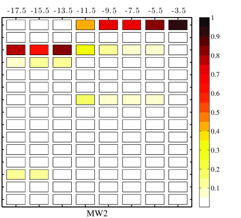
It is interesting to repeat this analysis using different dark matter-only simulations to explore how the formation history of the host galaxy may affect our results. For this purpose we have computed the ANOVA decompositions of model emulators from training sets obtained after coupling ChemTreeN with different galaxy formation histories. In all cases, the same design was used to create the training sets, which consisted of $n=500$ points. In Figure 6 we show the results obtained by performing an ANOVA decomposition on the luminosity function outputs with the simulations MW1 and MW2 (the two remaining simulations yielded similar results, and thus we omit the figures showing them from this paper). Interestingly, the decompositions show, qualitatively, no substantial difference in all the formation histories considered. Although the fractions of the variance explained by the different parameters may slightly vary from one simulation to another, the parameters that are dominant remain the same for all model outputs. This highlights an important property of this kind of analysis: The ANOVA decomposition allows us to characterize the relationship between the input parameters and the desired model outputs, independently of the corresponding real observable values and the underlying formation history of our galactic model. Note however that, while the ANOVA decompositions are equivalent in all formation histories, the actual values of the model outputs can (and typically do) differ from emulator to emulator.

Comparison of Figure 3 and the left panel of Figure 6 shows that the results were not altered by either reducing the dimensionality of the problem or by considering a different training set. To test for convergence, we have used a random sub-sample of $n=300$ training models to compute the ANOVA decomposition of model MW1. The resulting decomposition showed no significant differences with respect to that obtained with $n=500$ points.

5. Searching for best-fitting parameter regions in a multidimensional space

Figure 7.— Top panels: Different sections of the joint implausibility surface, $J_{1}(\mathbf{x})$. The different colors show different values of $J_{1}(\mathbf{x})$ in logarithmic scale. Model emulators are compared to values of the mock observable Luminosity Function (LF) obtained after running ChemTreeN with the fiducial parameter values. Both the mock observables and the training data set are obtained by coupling ChemTreeN with the N-body simulation MW1. The fiducial values of the corresponding parameters are indicated with a blue circle The horizontal black solid line on the color bar indicates the imposed threshold: a value above this threshold shows that it is very implausible to obtain a good fit to the observed data with the corresponding values of the model parameters. Bottom panels: Two dimensional projected densities of the DRAM chain points, obtained after marginalizing the samples of the five dimensional likelihood, $\mathcal{L}_{1}(\mathbf{x})$ (see equation 14), over the remaining three dimensions. The samples have been smoothed and contoured to aid the eye. In all projections the posterior density has been normalized by its maximum value. The most plausible regions of input parameter space are shown as the highest density peaks.

Figure 8.— As in the bottom middle panel of Figure 7, obtained after only considering chain points located within a restricted range of $z_{\rm r}$, centered around its fiducial value. The corresponding range is indicated in the top right corner of the panel.

Figure 9.— As in Figure 7, when values of the corresponding Metallicity Functions (MFs) are considered as mock observables.

The sensitivity analysis performed in the previous section allowed us to identify the set of input parameters that, given the selected observables, could be significantly constrained. In this section we introduce a technique to efficiently identify best-fitting input parameter regions when dealing with multidimensional spaces, $p>3$.

To explore the robustness of the method we will first consider a set of mock observables obtained after coupling ChemTreeN with the simulation MW1. The values of the parameters used to generate this model, and those we will try to recover, are listed in Table  2 as the fiducial model values. These values were previously used by T10 to fit reasonably well several properties of the Galactic stellar halo. As discussed in G12, best fitting parameters could in principle be identified by searching for regions of low values of the joint implausibility measure, $J(\mathbf{x})$ (see Equation (6)). In low dimensionality input parameter spaces, $p\leq 3$, this goal can be achieved simply by slicing the resulting $J(\mathbf{x})$ data cube. However, for higher dimensional spaces this task becomes unfeasible. Instead, to explore the input parameter space we will use a Delayed Rejection Adaptive Metropolis (DRAM) sampling method. DRAM is the result of combining two powerful methods, i.e. Delayed Rejection and Adaptive Metropolis, to improve the efficiency of Metropolis-Hastings type Markov Chain Monte Carlo (MCMC) algorithms (for details about this method, see Haario et al., 2006).

We start by constructing Gaussian process model emulators considering a five-dimensional input parameter space that includes the parameters $\mathbf{x}=\left(z_{\rm r},~{}f_{\rm bary},~{}f_{\rm esc},~{}\epsilon_{*},~{}\epsilon_{\rm SN}\right)$. We create a training set consisting of $n=500$ points. Note that, as previously discussed, a design with a smaller number of points could have been considered. However, this relatively large number of design points provides more accurate emulators within a reasonable run time. The black solid lines in Figure 1 show the cumulative functions extracted from our fiducial model.

The outputs from our Gaussian process model emulators and the set of mock observables are used to compute the joint implausibility measure $J(\mathbf{x})$, shown in Figure 7 . In the top panels we show two-dimensional sections of the $J_{1}(\mathbf{x})$ data hypercube, where the sub index 1 indicates that the training set used to build the emulators was obtained after coupling ChemTreeN with the dark matter simulation MW1. Note that these sections are the result of slicing the hypercube through the known fiducial values of the remaining three parameters. In each panel, the fiducial values of the two remaining parameters are indicated with a blue circle. As expected from the ANOVA decomposition shown in Figure 3, with this set of mock observables it is possible to strongly constrain the parameters $z_{\rm r}$ and $f_{\rm bary}$ (as shown in the top left panel). Note that the most plausible regions enclose the fiducial values of these parameters. The top middle panel of Figure 7 shows that an equally good fit to the luminosity function can be obtained for a large range of $\epsilon_{*}$ values. Clearly, constraints on this parameter are significantly weaker. Note also that the remaining two parameters, $f_{\rm esc}$ and $\epsilon_{\rm SN}$, are very poorly constrained (top right panel).

In reality, the values of the parameters that could best reproduce the (real) observables are all unknown. As previously discussed, slicing the resulting multidimensional data cube to search for regions of low $J(\mathbf{x})$ values becomes unfeasible for values of $p>3$. To explore the input parameter space we use the DRAM sampling method. The likelihood used by the DRAM is

$$\mathcal{L}_{1}(\mathbf{x})\propto e^{-J_{1}(\mathbf{x})^{2}/2},$$ (14)

where we have assumed a multivariate normal distribution and uniform prior for all parameters. Note that the assumed priors could be easily modified to account for any previous knowledge about the input parameters’ values. Nonetheless, as we show later in Section 6, the choice of uniform priors is important if we want to characterize the dependence of the “best fitting” parameter selection process on the merger histories of the adopted Milky Way-like models. The resulting joint posterior distributions are shown in the bottom panels of Figure 7. The DRAM chains presented in this work consist of $5\times 10^{5}$ points. Convergence of these chains was assessed by diagnostics such as the Geweke test (Geweke, 1992). Each panel presents contours of the projected density of points, $\rho$, obtained from the DRAM chain. The two-dimensional projected densities represent the result of marginalizing the DRAM chain samples over the remaining three dimensions. For comparison, in all cases we have normalized $\rho$ to it maximum value, $\rho_{0}$. The most plausible regions of input parameter space are shown as the highest density peaks. Note that the fiducial values of the parameters $z_{\rm r}$, $f_{\rm bary}$, and $\epsilon_{*}$ are located within the highest density regions. As expected, however, the parameters $z_{\rm r}$ and $f_{\rm bary}$ are significantly more strongly constrained than $\epsilon_{*}$. To explore whether spurious structure in these density contours could be induced due to auto-correlation in the chain, we have split the chain into five different “subchains”. This thinning of the chain was done by taking one out of every five points, with a different starting point taken from the first five elements of the total chain. In all cases, the results were not affected by this sub-sampling (see Link & Eaton, 2012, for an interesting discussion on thinning).

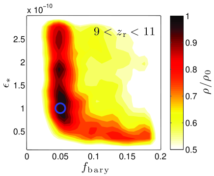
In general, the shape of the density contours is very similar to that of the $J_{1}(\mathbf{x})$ sections, shown on the top panels. It is important to note that the DRAM chain density contours are obtained after fully sampling the five-dimensional input parameter space, without any prior knowledge of the fiducial values of the parameters. To obtain these two-dimensional density contours we are implicitly averaging over all the variations in the three remaining directions. Instead, to compute the two-dimensional $J_{1}(\mathbf{x})$ sections, the $J_{1}(\mathbf{x})$ hypercube was sliced at the fiducial values of the remaining three parameters. Thus, prior knowledge of these parameters’ values was required. A similar idea can be applied to the DRAM chain density to improve the constraint on the star formation efficiency, $\epsilon_{*}$. As previously discussed, the bottom left panel of Figure 7 imposes strong constraints on the redshift of the epoch of reionization, $z_{r}$. In Figure 8 we show DRAM density contours in $f_{\rm bary}$ and $\epsilon_{*}$ space, obtained after only considering chain points located within a restricted range of $z_{\rm r}$, centered around its fiducial value. The chosen range, $9<z_{\rm r}<11$, is large enough to fully include the high density region shown on the bottom left panel of Figure 7. Note that as a result of choosing this reasonable range in $z_{\rm r}$, both $f_{\rm bary}$ and $\epsilon_{*}$ are significantly better constrained.

In Figure 9 we show $J_{1}(\mathbf{x})$ sections (top row), and the corresponding DRAM chain density contours (bottom row), obtained when values of the metallicity function are considered as mock observables. The ANOVA decomposition shown in Figure 5 indicated that, in our models, a significant fraction of the variability observed in these model outputs is associated with variations of the parameters $z_{\rm r}$, $f_{\rm esc}$, and $\epsilon_{\rm SN}$. Indeed, the $J_{1}(\mathbf{x})$ sections show that constraints to these parameters can be obtained when these mock observables are considered. This is especially relevant for the pair of parameters $f_{\rm esc}$ and $\epsilon_{\rm SN}$, which could not be constrained by the luminosity function. Note that the corresponding section (middle panel) unveils a non-linear relation between these two parameters, with several “islands” of very low implausibility (i.e., high probability). In each section, the fiducial values of corresponding pairs of parameters are indicated with a blue circle. As previously shown for the luminosity function, these parameters can be significantly constrained without any prior knowledge of the parameters’ fiducial values thanks to the DRAM chain sampling.

Figure 10.— Cumulative number of satellite galaxies as a function of absolute V-band magnitude, M_v. The top panel shows the results obtained when the input parameters are fixed to the fiducial values, listed in Table  2. The bottom panel shows the results obtained when the input parameters are fixed at $\mathbf{x}_{\rm hd}^{i}$, the highest density peak of the corresponding DRAM chain (see Table  3). In both panels, the black stars show the luminosity function of observed Milky Way satellite galaxies corrected for incompleteness as described by Koposov et al. (2008). The bars indicate Poisson noise error.

6. Applications to the Milky Way: A method to constrain its assembly history

Figure 11.— Projected densities of DRAM chain points obtained from our different MW$i$ models, with $i=1,2,3$ and 4. The color-coded contours show the results obtained with a different likelihood function, $\mathcal{L}_{i}(\mathbf{x})$. Starting from the densest point of each final distribution, $\mathbf{x}^{i}_{\rm hd}$, the different contour levels enclose 1, 5 and 10 per cent of corresponding DRAM-chain points. The color-coded dot indicates the location of $\mathbf{x}^{i}_{\rm hd}$, whereas the black dots indicate the location of the parameter’s fiducial values. The black square indicates the ‘best-fit’ model from Tumlinson (2010).

In G12 we showed that the best-fitting input parameter selection process strongly depends on the underlying merger history of Milky Way-like galaxy used to train the model emulators. In this section we will show how this characteristic of our method could be used to constrain the assembly history of the Milky Way and its properties at $z=0$. Our approach consists of obtaining a best-fitting model for each Milky Way-like dark matter halo being considered. The best-fit parameters are allowed to freely vary from model to model. The resulting best-fit model is then compared with a second and independent observational data set that can then be used to evaluate its reasonableness. As we will show in what follows, it is always possible to find a set of input parameters to tightly reproduce a given observational data set. However, only some of these best-fit models are successful at reproducing a second and independent set of observables. The results from the sensitivity analysis presented in Section 4 will allow us to focus our analysis on the parameters that have the largest impact on the predictions of the selected observables. The DRAM method will allow us to quickly explore the resulting joint implausibility hypercubes to identify regions of best fitting input parameter sets.

The observables that are considered in this Section are extracted from the real Milky Way galaxy’s satellite distribution. These are the luminosity function of satellite galaxies located within 280 kpc, corrected for incompleteness as described by Koposov et al. (2008), and the cumulative metallicity function. Values for the $\langle$[Fe/H]$\rangle$ of all dwarfs were extracted from the data compilation presented by McConnachie (2012). Note that, thus far, the fiducial model and the training set shared the same galaxy’s formation history, associated with the simulation MW1. The formation history of the Milky Way is of course an unknown in our search for the best-fitting parameters.

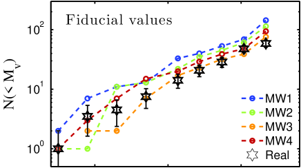
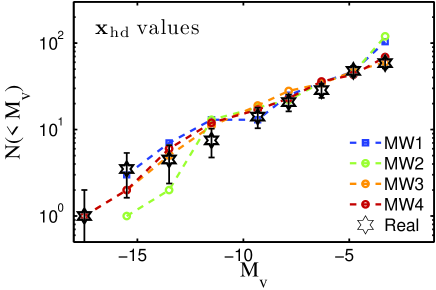
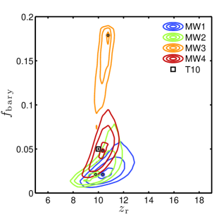
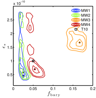
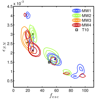
Figure 10 shows, with black stars, the luminosity function of the Milky Way’s satellite galaxies (McConnachie, 2012). For comparison, the color-coded dashed lines show the luminosity function of the models with the fiducial parameters. These models were obtained after coupling ChemTreeN with the four dark matter-only cosmological simulations MW$i$ (with $i=1,2,3$ and 4), and fixing the input parameters at the fiducial values listed in Table  2. The four models show significant deviations from the data. It is thus likely that for each Milky Way dark matter halo model there exists a small volume of input parameter space within which a better fit to the observed luminosity function can be obtained. To search for this volume we employ the DRAM sampling technique previously described. We train model emulators using four different training sets. The sets are the results of coupling ChemTreeN to the four dark matter-only cosmological simulations of Milky Way-size galaxies. The same design for each simulation, consisting of $n=500$ points, was used. For each set of model emulators, trained on a different MW$i$, we obtained a different joint implausibility function $J_{i}(\mathbf{x})$ (see eqn (6)). These $J_{i}(\mathbf{x})$ are the result of comparing the outputs of the model emulators to the real observable data. We use the $J_{i}(\mathbf{x})$ to construct four different likelihood functions $\mathcal{L}_{i}(\mathbf{x})$ (see eqn. 14). Figure 11 shows the results of the DRAM sampling. The left panel show contours of the projected density of DRAM chain points in $(z_{\rm r},f_{\rm bary})$ space. The different colored contours shows the results obtained with the four different $\mathcal{L}_{i}(\mathbf{x})$. Starting from the densest point of each final distribution, $\mathbf{x}^{i}_{\rm hd}$, the different contour levels enclose 1, 5 and 10 per cent of corresponding DRAM chain points. The color-coded dot indicates the location of $\mathbf{x}^{i}_{\rm hd}$. Note that strong constraints on the parameters $(z_{\rm r},f_{\rm bary})$ are obtained for the four MW$i$. Let us recall that the satellite luminosity function is most sensitive to this pair of input parameters. Interestingly, except for the model MW4, the locations of $\mathbf{x}^{i}_{\rm hd}$ are significantly off from the fiducial values, especially in the direction of $f_{\rm bary}$. The values of the parameters associated with $\mathbf{x}^{i}_{\rm hd}$ are listed in Table  3. The most extreme case is given by halo MW3, where the most plausible value of $f_{\rm bary}$ is approximately four times larger than the fiducial value. Note that, as shown in the top panel of Figure 10, when compared with the Milky Way luminosity function this model (obtained with the fiducial parameters) presents a significant deficit of bright satellites. On the other hand, MW1’s model shows an excess of satellites at all magnitudes. Note that the most plausible value of $f_{\rm bary}$ obtained by the DRAM sampling in this case is approximately two times lower than the fiducial value. To explore whether the location of $\mathbf{x}^{i}_{\rm hd}$ depends on the number of points used in the DRAM sampling, we divided the final chains into five different subchains as described in Section 5. From each sub-chain we obtained the corresponding location of $\mathbf{x}^{i}_{\rm hd}$ and computed its average value, $\langle\mathbf{x}^{i}_{\rm hd}\rangle$. We find that, in all cases, $\langle\mathbf{x}^{i}_{\rm hd}\rangle$ is in excellent agreement with the values of $\mathbf{x}^{i}_{\rm hd}$ obtained from the full chain. In most cases the associated standard deviation is negligible. Furthermore, as we will show below our results are not significantly affected by small variations in $\mathbf{x}^{i}_{\rm hd}$. The middle panel of Figure 11 shows contours of the projected density of DRAM-chain points in the $(f_{\rm bary},\epsilon_{*})$ space. Following the discussion in Section 5, to obtain these contours we only considered chain points that are located within a specific range of $z_{\rm r}$, centered around the value associated with $\mathbf{x}^{i}_{\rm hd}$. The range of $z_{\rm r}$ chosen for each MW${i}$ is such that it includes all chain points that are located within the regions defined by the 10 per cent contour levels, shown in the left panel of Figure 11. Constraints on $\epsilon_{*}$ are weaker than those found for the pair $(z_{\rm r},f_{\rm bary})$. Multiple plausible regions of parameter space are found for almost all MW$i$ . The values of $\epsilon_{*}$ associated with $\mathbf{x}^{i}_{\rm hd}$ show a large scatter and, as before, it gets closer to the fiducial value for MW4.

Table 3Model parameter extracted from the highest density peak of the corresponding DRAM-chain’s posterior density.

Name	$z_{\rm r}$	$f_{\rm esc}$	$f_{\rm bary}$	$\epsilon_{*}$	$\epsilon_{\rm SN}$	$M_{40}$
$\text{MW}{1}$	10.3	57.7	0.021	0.4 $\times 10^{-10}$	0.00165	0.57
$\text{MW}{2}$	9.6	27.0	0.021	0.5 $\times 10^{-10}$	0.00304	0.95
$\text{MW}{3}$	10.7	19.1	0.168	17 $\times 10^{-10}$	0.00255	20.9
$\text{MW}{4}$	10.3	27.0	0.048	0.7 $\times 10^{-10}$	0.00211	1.88

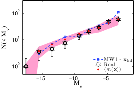
The bottom panel of Figure 10 shows the luminosity functions obtained after fixing the values of the input parameters at $\mathbf{x}^{i}_{\rm hd}$. The values of $(f_{\rm esc},\epsilon_{\rm SN})$ are kept fixed at the fiducial values, as the luminosity function is insensitive to variation of these parameters (see Figures 3 and 6). It is clear that, in all cases, a much better fit to the observed luminosity function is obtained with the sets of most-likely parameters derived from our DRAM chains. We now explore how sensitive this result is to the exact location of $\mathbf{x}^{i}_{\rm hd}$. For model MW1, we select the $\approx 2.5\times 10^{4}$ DRAM points that are located within the 5 per cent contour shown in Figure 11, and obtain a predicted luminosity function for each these points. Note that no restrictions are applied to the parameters $(\epsilon_{*},f_{\rm esc},\epsilon_{\rm SN})$. The resulting luminosity function computed by averaging all these points is shown in Figure 12 with red dots. The red shaded area indicates the $95\%$ confidence interval. A very good fit to the observed luminosity function is also obtained in this case, indicating that our results are not strongly sensitive to the exact location of $\mathbf{x}^{i}_{\rm hd}$.

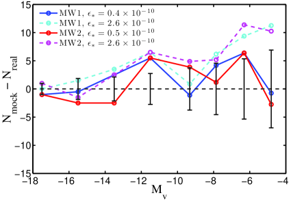
A good fit to the luminosity function, however, does not imply that the four resulting models, associated with the different MW$i$s, are equally good at reproducing simultaneously both the luminosity function of Milky Way dwarf satellites and the properties of the Milky Way stellar halo. As an example, we compare the mass of the corresponding stellar halos within $1-40$ kpc, $M_{40}$ with its observationally-determined value for the Milky Way. Using the Sloan Digital Sky Survey (SDSS), Bell et al. (2008) estimated a mass of $M_{40}=(3.7\pm 1.2)\times 10^{8}~{}M_{\odot}$ for the Milky Way stellar halo. The values of $M_{40}$ in our four best-fitting models are listed in Table  3. Interestingly, models MW1 and MW2 present an $M_{40}$ that is significantly smaller than the observationally-determined value, whereas MW3 suggests a much larger value. The simulated $M_{40}$ is comparable to its observational counterpart only for MW4. Note that this result even holds when fixing the value of the less well-constrained parameter, $\epsilon_{*}$, to its fiducial value. Models MW1, MW2 and MW3 are thus less likely to represent a good model of the Milky Way and its underlying formation history than MW4. Nonetheless, as previously discussed, constraints on $\epsilon_{*}$ are poor and thus multiple high density regions with different values of this parameter can be seen in the middle panel of Figure 11. This is especially true for models MW1 and MW2. As an example, we consider for these two models the high density peak located at $\epsilon_{*}\approx 2.6\times 10^{-10}$. This is the largest plausible value of $\epsilon_{*}$ for both models. The modeled $M_{40}$ obtained are $2.4$ and $3$ $\times 10^{8}~{}M_{\odot}$ for MW1 and MW2, respectively. Whereas model MW1 cannot match the observed $M_{40}$ even with this extreme value of $\epsilon_{*}$, model MW2 shows a better match. The luminosity functions obtained with both, i.e., the largest plausible value and that associated with $\mathbf{x}_{\rm hd}$, show good fits to the observed luminosity function. However, the former results in a slightly poorer fit. This is shown in Figure 13, where we plot the residuals of the luminosity functions, $N_{\rm mock}-N_{\rm real}$, for both values of $\epsilon_{*}$. Note that, in general, the luminosity functions associated with the larger plausible values of $\epsilon_{*}$ tend to overpredict the number of faint satellite galaxies.

The analysis just performed has the potential to allow us to constrain the Milky Way’s formation history and its properties at $z=0$. As discussed in Section 2.1, the four halos analyzed in this work were specially targeted to resemble the Milky Way. That is, they all have a very similar virial masses and have not experienced a major merger after approximately $z=1.5-2$. Their growth as a function of time is shown in Figure 4 of G12. Some differences can be easily observed. For example, our best-fitting model associated with halo MW4 has experienced the most significant late accretion. However, our sample of Milky Way-like dark matter halos is very small and thus we are strongly undersampling the range of possible merger histories of the Milky Way-like candidates. A much larger sample is required to determine whether any particular features observed in a halo’s assembly history are statistically significant. Nonetheless, using the set of simulations from the Aquarius project (Springel et al., 2008), Starkenburg et al. (2013) (hereafter S13) find that the number of luminous satellite galaxies brighter than $M_{\rm v}=-5$ within the virial radius of the host shows a significant correlation with the host’s dark matter halo virial mass. As discussed by S13, Macciò et al. (2010) also observed this trend and remarked that it does not depend on the particular semi-analytical model used. As shown in the top panel of Figure 10, the same behavior is observed in our simulations. Let us recall that this panel shows the luminosity functions of our four Milky Way-like models obtained after fixing the input parameters to their fiducial values. Interestingly, our preferred best fitting model, MW4, which can simultaneously reproduce the number of bright satellites with $M_{\rm v}\leq-5$ (see bottom panel of Figure 10), and can provide a reasonable estimate of $M_{40}$, has a value of $M_{\rm vir}=1.44\times 10^{12}$ $M_{\odot}$. This value is in good agreement with recent estimates of the total Milky Way mass (Gnedin et al., 2010; Boylan-Kolchin et al., 2013; Kallivayalil et al., 2013; Piffl et al., 2013). Within our framework, lower mass halos such as MW3, with an $M_{\rm vir}=1.22\times 10^{12}$ $M_{\odot}$, would be ruled out.

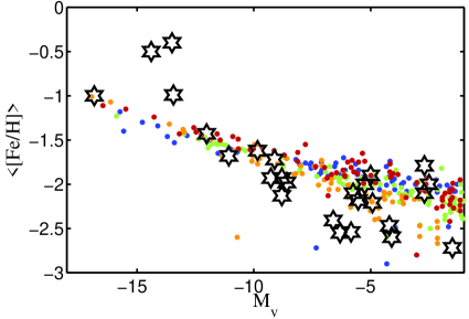
In Figure 14 we show, with black stars, the luminosity-metallicity (L-Z) relation of Milky Way satellites. Due to incompleteness in our current sample of observed satellite galaxies, and uncertainties on $\langle$[Fe/H]$\rangle$ measurements, it is not possible to derive a complete metallicity function relation down to $\langle$[Fe/H]$\rangle=-2.2$. The sample is severely incomplete at the metal-poor (and faint) end of the metallicity function. Thus, in order to compare with our models, we derive a metallicity function only taking into account satellite galaxies more metal-rich than $\langle$[Fe/H]$\rangle\geq-1.5$. This limit on $\langle$[Fe/H]$\rangle$ imposes a limit on M${}_{\rm v}\lesssim-11$ (see Figure 14), i.e., within the realm of the classical dwarfs. Following Tollerud et al. (2008), we assume that all satellites within this magnitude range should have been discovered anywhere in the sky, with the possible exception of objects at low Galactic latitudes where Milky Way extinction and contamination become significant (Willman et al., 2004).

In practice, we train a model emulator considering only two bins of the metallicity function, at $\langle$[Fe/H]$\rangle=-1.1$ and -1.5. As shown by the ANOVA decomposition in Figure 5, the number of satellites in these bins is very sensitive to variations of the escape factor of metal, $f_{\rm esc}$. Variation of the remaining parameters does not account for a very significant fraction of the variance obtained for these observables. The most metal-poor bins that we are omitting from this analysis are very sensitive to the redshift of the epoch of reionization, $z_{\rm r}$. The lack of the additional constraints provided by these metal-poor bins could induce the detection of spurious high density peaks in the DRAM density contours associated with values of $z_{\rm r}$ that do not represent the real data. To avoid this, we update the range of the uniform prior assigned to $z_{r}$ in our DRAM sampling analysis. This update is done based on the results obtained from the independent observational data set associated with the luminosity function. The new range for our $z_{\rm r}$ uniform priors is such that, in all cases, it includes the region of $z_{\rm r}$ enclosed within the 10 percent contours shown in the left panel of Figure 11. In the right panel of the same figure we show contours of the projected density of DRAM chain points in the $(f_{\rm esc},\epsilon_{\rm SN})$ space. As previously seen in Figure 5, a non-linear relation with several high density peaks regions is obtained in all four models. For a given value of $\epsilon_{\rm SN}$, models MW3 and MW4 require a lower value of $f{\rm esc}$ than models MW1 and MW2 to fit the observed metallicity function. The values of the parameter associated with the highest density peak, $\mathbf{x}_{\rm hd}^{i}$, are indicated with colored dots and listed in Table  3. However, we remind the reader that these values should be taken with caution due to the large uncertainties in the observable quantities. In Figure 14 we show the L-Z relation of the models obtained after fixing the input parameters at $\mathbf{x}_{\rm hd}^{i}$. Note that, in all cases, a very good fit to the observed L-Z relation is obtained.

7. Discussion and Conclusions

In this paper we have presented a novel application of the statistical tool known as sensitivity analysis to characterize the relationship between input parameters and observational predictions for the chemo-dynamical galaxy formation model ChemTreeN. In particular, we focus on efforts to model the Milky Way stellar halo and its population of satellite galaxies. ChemTreeN is a semi-analytic model of galaxy formation that has been coupled to cosmological simulations that provide realistic merger histories and phase space distribution of the resulting stellar populations.

The implementation of a semi-analytic model involves the fine-tuning of a large number of free parameters that control the behavior of many different physical processes, and the choice of a “best fit” parameter selection may be quite challenging. The process of choosing these parameters generally involves the comparison of a given observational data set with the corresponding model outputs. Due to the complexity of galaxy formation models, and the non-linear coupling between physical prescriptions in the model, it is typically non-trivial to predict how variations of parameters or groups of parameters can affect a given model output. We have addressed this problem by implementing a sensitivity analysis, which decomposes the relationship between input parameters and predicted observable properties into different “effects.” Each effect characterizes how an output responds to variations of only a subset of input parameters, and thus can be used to inform the user of which parameters are most important and most likely to affect the prediction of a given observable. Conversely, this sensitivity analysis can also be used to show what model parameters can be most efficiently constrained by a given observational data set. Finally, this analysis can allow modelers to simplify their models, or at the very least ignore specific parameters for the purposes of a given study, by identifying input parameters that have no affect on the outputs (i.e., observational predictions) of interest.

Figure 12.— Cumulative number of satellite galaxies as a function of absolute V-band magnitude, M_v. The black stars show the luminosity function of observed Milky Way satellite galaxies corrected for incompleteness as described by Koposov et al. (2008). The bars indicate Poisson errors. The blue dashed line shows, for model MW1, the luminosity function obtained when the input parameters are fixed at $\mathbf{x}_{\rm hd}^{i}$, the highest density peak of the corresponding DRAM chain (see Table  3). The red dots show the mean luminosity function obtained after averaging the prediction of the model emulator for all DRAM points within the 5 per cent contour shown in Figure 11. The red shaded area show the $95\%$ confidence interval.

Figure 13.— Residual luminosity functions obtained after subtracting the real luminosity function from the results of different models. The solid lines indicate the results obtained when the value of $\epsilon_{*}$ associated with $\mathbf{x}_{\rm hd}$ is considered. The dashed lines show the results obtained when the largest plausible value of $\epsilon_{*}$ is considered. The horizontal black dashed line indicates a perfect fit to the observed luminosity function. The errors bars indicate Poisson errors.

Figure 14.— Luminosity-metallicity (L-Z) relation of satellite galaxies. The black stars show the Milky Way L-Z relation, as presented by McConnachie (2012). The color-coded dots show the results obtained from our four models after fixing ChemTreeN’s input parameters at $\mathbf{x}_{\rm hd}^{i}$, the highest-density peak of the corresponding DRAM chain (see Table  3)

When applying a sensitivity analysis it is necessary to densely sample one’s model over the whole range of interest of its input parameter space. With the ChemTreeN code, doing this rapidly becomes computationally prohibitive as the dimensionality of the input parameter space increases (with each model requiring between minutes and hours to complete). To circumvent this problem, we have trained statistical model emulators based on Gaussian processes. These emulators act as an approximate (but reasonably accurate) representation of the outputs of the ChemTreeN code and are very computationally efficient, running in substantially less than a millisecond, as opposed to hours for a ChemTreeN model. This makes it feasible to predict vast numbers of model outputs in a short period of time. While the Gaussian process emulator is an approximation of the outputs from ChemTreeN, it is reasonably accurate when constructed correctly (as discussed in Gómez et al., 2012a)), and provides both an estimate of the output values and their error (which is useful when comparing the models to observational data).

We have also shown how the results of a sensitivity analysis can be easily visualized thanks to the ANOVA decomposition. The ANOVA decomposition provides a way to quantitatively measure the percentage of the total output parameter variance that can be explained by either variations of single input variables or by any combination of two or more input variables.

In the analysis performed in this paper, we have considered the Milky Way satellite galaxy cumulative luminosity and metallicity functions. Our work shows that, when the luminosity function is used as the sole observational data set, the parameters that could be most strongly constrained in ChemTreeN are: i) the onset of the epoch of reionization, $z_{\rm r}$, ii) the baryonic mass fraction assigned to each dark matter halo, i.e. the baryon accretion rate, $f_{\rm bary}$, and iii) to a much lesser extent, the star formation efficiency, $\epsilon_{*}$. The decomposition also showed that the bright end of the luminosity function is most sensitive to baryon accretion rate (and is essentially only sensitive to this quantity), and the faint end of the luminosity function is dominated by variation in the onset redshift of the epoch of reionization. We also find through the ANOVA decomposition that the luminosity function is entirely insensitive to variations of the input parameters that control the remaining physical prescriptions.

Considering the Milky Way satellite galaxy metallicity function as the observable data set allows us to put useful constraints on two additional parameters: the efficiency with which metals are ejected from galaxies, $f_{\rm esc}$, and the efficiency of the coupling of supernova explosions with the interstellar medium within a galaxy (and thus their energy deposition rates), $\epsilon_{\rm SN}$. Interestingly, we find that these two prescriptions are strongly non-linearly coupled. The cumulative number of metal-rich satellite galaxies (defined here to be $\langle$[Fe/H]$\rangle\geq-1.1$) is strongly dominated by the fraction of metals ejected out of the host galaxy due to supernova-driven winds. There is also a weaker dependence on the efficiency of the supernova energy coupling, $\epsilon_{\rm SN}$, and on the redshift of reionization, $z_{\rm r}$. As we move toward lower values of $\langle$[Fe/H]$\rangle$ the cumulative number of satellite galaxies becomes strongly sensitive to the redshift of the epoch of reionization.

It is important to remark that the ANOVA decomposition allows us to characterize the relationship between the input parameters and the desired model outputs independent of the corresponding real observable values and the underlying formation history of our galactic model. In other words, the relative relationship between the model’s input and output parameters is approximately independent of, and thus separable from, the underlying galaxy merger history – a very useful result that can help to inform choices regarding the quantity and properties of relatively expensive cosmological simulations. As a consequence of our ANOVA analysis, we were able to reduce the dimensionality of the model’s input parameter space from seven dimensions to the five dimensions that actually had an impact on the selected observables, and then to apply this reduced-dimensionality model to our suite of cosmological simulations.

By defining a statistical measure of plausibility, and by comparing model emulators to mock observational data in a quantitative manner, we have demonstrated that it is possible to recover the input parameter vector used to create the mock observational data set even when no prior knowledge of the input parameter is provided. The search of the best-fitting parameter volume required the use of a Delayed Rejection Adaptive Metropolis (DRAM) method to sample the whole input parameter space. The involved likelihood function was based on the (im)plausibility measure defined in Section 3. A different choice of implausibility measure (i.e., different means of determining goodness-of-fit of the model and observational data) may affect our results in a quantitative sense, but is unlikely to make a qualitative difference in results for the observational quantities that we have chosen.

We have applied this statistical machinery to real observational data sets associated with the Milky Way – namely, the luminosity and metallicity functions of our galaxy’s dwarf satellites. As we showed in G12, the best-fitting input parameter selection process strongly depends on the underlying merger history of Milky Way-like galaxy used to train the model emulators. In this work we discussed how this characteristic of our method could be used to constrain the assembly history of the Milky Way and its properties at $z=0$. Our approach consisted of obtaining a best fitting model for each Milky Way-like dark matter halo being considered. The best-fit parameters were allowed to freely vary from model to model. In the four cases considered, the Milky Way satellite luminosity function allowed us to put strong constraints not only on the baryon accretion rates, but also on how long the less massive galaxies were able to accrete gas before reionization shut them down. The best-fitting parameters showed significant scatter between cosmological simulations, especially along the direction of the baryon fraction, $f_{\rm bary}$. The resulting best-fit models provided a luminosity function that tightly fit their observed counterpart in all cases. However, only one of our models was able to reproduce the observed stellar halo mass within 40 kpc of the Galactic center, $M_{40}$. The remaining three models showed values that are either substantially too large or too small when compared to the observed value. On the basis of this analysis it is possible to disregard these three models and their corresponding merger histories as good representations of the underlying merger history of the Milky Way. Interestingly, as previously observed by Macciò et al. (2010) and Starkenburg et al. (2013), the number of luminous satellite galaxies brighter than $M_{\rm v}=-5$ shows a significant correlation with the host’s dark matter halo virial mass. Our preferred best-fitting model, MW4, which can reproduce the number of bright satellites with $M_{\rm v}\leq-5$ and simultaneously provide a reasonable estimate of $M_{40}$, has a value of $M_{\rm vir}=1.44\times 10^{12}$ $M_{\odot}$. This is in good agreement with recent estimates of the total MW mass (Gnedin et al., 2010; Boylan-Kolchin et al., 2013; Kallivayalil et al., 2013; Piffl et al., 2013). Lower mass halos such as MW3, with $M_{\rm vir}=1.22\times 10^{12}$ $M_{\odot}$, would be ruled out within our framework. It is important to notice however that due to the relatively poor constraints obtained on the star formation efficiency, $\epsilon_{*}$, two of the models with different formation histories, namely MW1 and MW2, presented multiple likely values for this parameter. As an example, for these two models we computed the value of $M_{40}$ associated with the largest plausible value of $\epsilon_{*}$. Our results showed that, while one of the models was not able to reproduce the observed value of $M_{40}$ even in this case, the second resulted in a much better fit to the observed value. Nonetheless, in both cases the mock luminosity functions obtained with the largest plausible value of $\epsilon_{*}$ resulted in poorer fits to their observed counterpart than those obtained with the best fitting parameters. A more robust comparison could be achieved by contrasting the observed $M_{40}$ to the distribution of modeled $M_{40}$ associated with the 10 per cent most likely values of $f_{\rm bary}$ and $z_{\rm r}$ and their corresponding $\epsilon_{*}$. This is beyond the scope of this paper and we defer it to a future work.

Due to incompleteness in our current sample of satellite galaxies, as well as uncertainties on $\langle$[Fe/H]$\rangle$ measurements, results based on the metallicity function are significantly less certain. Incompleteness is a much greater problem for low mass (and thus low luminosity and low metallicity) satellites; so, to compare with our models we derive a metallicity function that only includes galaxies that are more metal-rich than $\langle$[Fe/H]$\rangle=-1.5$. This imposes a magnitude limit of M${}_{\rm v}\approx-11$, which is within the luminosity range of the classical dwarf galaxies. In the space defined by $f_{\rm esc}$ and $\epsilon_{\rm SN}$, the DRAM sampling of the implausibility hyper surface associated with this reduced set of galaxies resulted in several “islands” of high plausibility. The models associated with the best fitting parameters presented, in all cases, a luminosity-metallicity relation for satellite galaxies that agrees well with the observed relation over that magnitude range. However, due to large source uncertainties, no further constraints were obtained with this observational data set.

The results presented on this work are an example of a procedure that can be applied to statistically constrain the formation history of the Milky Way. A more robust and statistically significant analysis would require i) the addition of a large set of possible formation histories and ii) a direct comparison to a larger number of available observable quantities. To address the first point, we are currently running a large suite of high resolution dark matter-only cosmological simulations of the formation of Milky Way-like halos. These simulation will allow us to probe different galaxy formation histories, ranging from halos that acquire most of their mass very early on to halos that have had their last major merger episode close to $z=0$, and also the plausible range of masses that have been attributed to the Milky Way. The resulting best-fitting models associated with each formation history will be confronted by a much richer observational data set, including observable quantities such as mean halo metallicity and chemical abundances as a function of radius, radial distribution of satellite galaxies, and possibly even the degree of phase-space substructure. By using this iterative method, we hope to provide useful constraints on the Milky Way’s mass and formation history that are complementary to alternate theoretical techniques, and which provide insight both into our own Galaxy’s behavior and, more generally, into the process by which all galaxies form.

References

- Barden et al. (2010) Barden, S. C., et al. 2010, in Society of Photo-Optical Instrumentation Engineers (SPIE) Conference Series, Vol. 7735, Society of Photo-Optical Instrumentation Engineers (SPIE) Conference Series
- Bell et al. (2008) Bell, E. F., et al. 2008, ApJ, 680, 295
- Belokurov et al. (2006) Belokurov, V., et al. 2006, ApJ, 642, L137
- Belokurov et al. (2007) —. 2007, ApJ, 654, 897
- Belokurov et al. (2010) —. 2010, ApJ, 712, L103
- Benson (2010) Benson, A. J. 2010, Phys. Rep., 495, 33
- Benson (2012) —. 2012, NewA, 17, 175
- Bond et al. (2010) Bond, N. A., et al. 2010, ApJ, 716, 1
- Bower et al. (2006) Bower, R. G., Benson, A. J., Malbon, R., Helly, J. C., Frenk, C. S., Baugh, C. M., Cole, S., & Lacey, C. G. 2006, MNRAS, 370, 645
- Bower et al. (2010) Bower, R. G., Vernon, I., Goldstein, M., Benson, A. J., Lacey, C. G., Baugh, C. M., Cole, S., & Frenk, C. S. 2010, MNRAS, 407, 2017
- Boylan-Kolchin et al. (2013) Boylan-Kolchin, M., Bullock, J. S., Sohn, S. T., Besla, G., & van der Marel, R. P. 2013, ApJ, 768, 140
- Bullock & Johnston (2005) Bullock, J. S., & Johnston, K. V. 2005, ApJ, 635, 931
- Bullock et al. (2000) Bullock, J. S., Kravtsov, A. V., & Weinberg, D. H. 2000, ApJ, 539, 517
- Carollo et al. (2008) Carollo, D., et al. 2008, Nature, 451, 216
- Carollo et al. (2010) —. 2010, ApJ, 712, 692
- Cooper et al. (2010) Cooper, A. P., et al. 2010, MNRAS, 406, 744
- Corlies et al. (2013) Corlies, L., Johnston, K. V., Tumlinson, J., & Bryan, G. 2013, ApJ, 773, 105
- Cui et al. (2012) Cui, X.-Q., et al. 2012, Research in Astronomy and Astrophysics, 12, 1197
- Dekel & Woo (2003) Dekel, A., & Woo, J. 2003, MNRAS, 344, 1131
- Diemand et al. (2006) Diemand, J., Kuhlen, M., & Madau, P. 2006, ApJ, 649, 1
- Font et al. (2006) Font, A. S., Johnston, K. V., Bullock, J. S., & Robertson, B. E. 2006, ApJ, 638, 585
- Font et al. (2011) Font, A. S., McCarthy, I. G., Crain, R. A., Theuns, T., Schaye, J., Wiersma, R. P. C., & Dalla Vecchia, C. 2011, MNRAS, 416, 2802
- Frebel & Norris (2013) Frebel, A., & Norris, J. E. 2013, Metal-Poor Stars and the Chemical Enrichment of the Universe, ed. T. D. Oswalt & G. Gilmore, 55
- Geweke (1992) Geweke, J. 1992, in IN BAYESIAN STATISTICS (University Press), 169–193
- Gilbert et al. (2012) Gilbert, K. M., et al. 2012, ApJ, 760, 76
- Gilmore et al. (2012) Gilmore, G., et al. 2012, The Messenger, 147, 25
- Girardi et al. (2002) Girardi, L., Bertelli, G., Bressan, A., Chiosi, C., Groenewegen, M. A. T., Marigo, P., Salasnich, B., & Weiss, A. 2002, A&A, 391, 195
- Girardi et al. (2004) Girardi, L., Grebel, E. K., Odenkirchen, M., & Chiosi, C. 2004, A&A, 422, 205
- Gnedin (2000) Gnedin, N. Y. 2000, ApJ, 542, 535
- Gnedin et al. (2010) Gnedin, O. Y., Brown, W. R., Geller, M. J., & Kenyon, S. J. 2010, ApJ, 720, L108
- Gómez et al. (2012a) Gómez, F. A., Coleman-Smith, C. E., O’Shea, B. W., Tumlinson, J., & Wolpert, R. L. 2012a, ApJ, 760, 112
- Gómez et al. (2013) Gómez, F. A., Helmi, A., Cooper, A. P., Frenk, C. S., Navarro, J. F., & White, S. D. M. 2013, ArXiv e-prints
- Gómez et al. (2012b) Gómez, F. A., et al. 2012b, MNRAS, 423, 3727
- Greggio & Renzini (1983) Greggio, L., & Renzini, A. 1983, A&A, 118, 217
- Haario et al. (2006) Haario, H., Laine, M., Mira, A., & Saksman, E. 2006, Statistics and Computing, 16, 339
- Henriques et al. (2009) Henriques, B. M. B., Thomas, P. A., Oliver, S., & Roseboom, I. 2009, MNRAS, 396, 535
- Ivezić et al. (2008) Ivezić, Ž., et al. 2008, ApJ, 684, 287
- Jurić et al. (2008) Jurić, M., et al. 2008, ApJ, 673, 864
- Kallivayalil et al. (2013) Kallivayalil, N., van der Marel, R. P., Besla, G., Anderson, J., & Alcock, C. 2013, ApJ, 764, 161
- Keller et al. (2012) Keller, S. C., Skymapper Team, & Aegis Team. 2012, in Astronomical Society of the Pacific Conference Series, Vol. 458, Galactic Archaeology: Near-Field Cosmology and the Formation of the Milky Way, ed. W. Aoki, M. Ishigaki, T. Suda, T. Tsujimoto, & N. Arimoto, 409
- Kennedy & O’Hagan (2000) Kennedy, M. C., & O’Hagan, A. 2000, Biometrika, 1
- Kirby et al. (2011) Kirby, E. N., Lanfranchi, G. A., Simon, J. D., Cohen, J. G., & Guhathakurta, P. 2011, ApJ, 727, 78
- Klypin et al. (1999) Klypin, A., Kravtsov, A. V., Valenzuela, O., & Prada, F. 1999, ApJ, 522, 82
- Koposov et al. (2008) Koposov, S., et al. 2008, ApJ, 686, 279
- Kroupa (2001) Kroupa, P. 2001, MNRAS, 322, 231
- Link & Eaton (2012) Link, W., & Eaton, M. 2012, Methods in Ecology and Evolution, 3, 112
- Lu et al. (2012) Lu, Y., Mo, H. J., Katz, N., & Weinberg, M. D. 2012, MNRAS, 421, 1779
- Lu et al. (2013) Lu, Y., Mo, H. J., Lu, Z., Katz, N., & Weinberg, M. D. 2013, ArXiv e-prints
- Macciò et al. (2010) Macciò, A. V., Kang, X., Fontanot, F., Somerville, R. S., Koposov, S., & Monaco, P. 2010, MNRAS, 402, 1995
- Majewski et al. (2010) Majewski, S. R., Wilson, J. C., Hearty, F., Schiavon, R. R., & Skrutskie, M. F. 2010, in IAU Symposium, Vol. 265, IAU Symposium, ed. K. Cunha, M. Spite, & B. Barbuy, 480–481
- McConnachie (2012) McConnachie, A. W. 2012, AJ, 144, 4
- McConnachie et al. (2009) McConnachie, A. W., et al. 2009, Nature, 461, 66
- Monachesi et al. (2013) Monachesi, A., et al. 2013, ApJ, 766, 106
- Moore et al. (1999) Moore, B., Ghigna, S., Governato, F., Lake, G., Quinn, T., Stadel, J., & Tozzi, P. 1999, ApJ, 524, L19
- Mouhcine et al. (2005) Mouhcine, M., Rich, R. M., Ferguson, H. C., Brown, T. M., & Smith, T. E. 2005, ApJ, 633, 828
- Nomoto et al. (1997) Nomoto, K., Iwamoto, K., Nakasato, N., Thielemann, F.-K., Brachwitz, F., Tsujimoto, T., Kubo, Y., & Kishimoto, N. 1997, Nuclear Physics A, 621, 467
- Oakley & O’Hagan (2002) Oakley, J. E., & O’Hagan, A. 2002, Biometrika, 89, 769
- Oakley & O’Hagan (2004) —. 2004, Journal of the Royal Statistical Society: Series B (Statistical Methodology), 66
- O’Hagan (2006) O’Hagan, A. 2006, Reliability Engineering & System Safety, 91, 1290 , the Fourth International Conference on Sensitivity Analysis of Model Output (SAMO 2004) - SAMO 2004
- Perryman et al. (2001) Perryman, M. A. C., et al. 2001, A&A, 369, 339
- Piffl et al. (2013) Piffl, T., et al. 2013, ArXiv e-prints
- Radburn-Smith et al. (2011) Radburn-Smith, D. J., et al. 2011, ApJS, 195, 18
- Rasmussen & Williams (2005) Rasmussen, C. E., & Williams, C. K. I. 2005, Gaussian Processes for Machine Learning (Adaptive Computation and Machine Learning) (The MIT Press)
- Ruiz et al. (2013) Ruiz, A. N., et al. 2013, ArXiv e-prints
- Sacks et al. (1989) Sacks, J., Welch, W. J., Mitchell, T. J., & Wynn, H. P. 1989, Stat. Sci., 4, 409
- Santner et al. (2003) Santner, T. J., Williams, B. J., & Notz, W. 2003, The Design and Analysis of Computer Experiments
- Schonlau & Welch (2006) Schonlau, M., & Welch, W. J. 2006, Screening the Input Variables to a Computer Code Via Analysis of Variance and Visualization, ed. A. Dean & S. Lewis (New York: Springer New York)
- Siebert (2012) Siebert, A. 2012, in SF2A-2012: Proceedings of the Annual meeting of the French Society of Astronomy and Astrophysics, ed. S. Boissier, P. de Laverny, N. Nardetto, R. Samadi, D. Valls-Gabaud, & H. Wozniak, 121–127
- Smith et al. (2008) Smith, E. D., Szidarovszky, F., Karnavas, W. J., & Bahill, A. T. 2008, The Open Cybernetics & Systemics Journal, 2, 39
- Spergel et al. (2007) Spergel, D. N., et al. 2007, ApJS, 170, 377
- Springel (2005) Springel, V. 2005, MNRAS, 364, 1105
- Springel et al. (2008) Springel, V., et al. 2008, MNRAS, 391, 1685
- Starkenburg et al. (2013) Starkenburg, E., et al. 2013, MNRAS, 429, 725
- Steinmetz et al. (2006) Steinmetz, M., et al. 2006, AJ, 132, 1645
- Tammann et al. (1994) Tammann, G. A., Loeffler, W., & Schroeder, A. 1994, ApJS, 92, 487
- Tissera et al. (2013a) Tissera, P., Beers, T., Carollo, D., & Scannapieco, C. 2013a, ArXiv e-prints
- Tissera et al. (2013b) Tissera, P. B., Scannapieco, C., Beers, T. C., & Carollo, D. 2013b, MNRAS, 432, 3391
- Tollerud et al. (2008) Tollerud, E. J., Bullock, J. S., Strigari, L. E., & Willman, B. 2008, ApJ, 688, 277
- Tominaga (2009) Tominaga, N. 2009, ApJ, 690, 526
- Tumlinson (2006) Tumlinson, J. 2006, ApJ, 641, 1
- Tumlinson (2010) —. 2010, ApJ, 708, 1398
- Wang et al. (2013) Wang, J., Frenk, C. S., & Cooper, A. P. 2013, MNRAS, 429, 1502
- Widrow et al. (2012) Widrow, L. M., Gardner, S., Yanny, B., Dodelson, S., & Chen, H.-Y. 2012, ApJ, 750, L41
- Williams et al. (2013) Williams, M. E. K., et al. 2013, MNRAS
- Willman et al. (2004) Willman, B., Governato, F., Dalcanton, J. J., Reed, D., & Quinn, T. 2004, MNRAS, 353, 639
- Yanny et al. (2009) Yanny, B., et al. 2009, AJ, 137, 4377
- York et al. (2000) York, D. G., et al. 2000, AJ, 120, 1579