Learning Mixtures of Linear Classifiers
Abstract
We consider a discriminative learning (regression) problem, whereby the regression function is a convex combination of linear classifiers. Existing approaches are based on the EM algorithm, or similar techniques, without provable guarantees. We develop a simple method based on spectral techniques and a ‘mirroring’ trick, that discovers the subspace spanned by the classifiers’ parameter vectors. Under a probabilistic assumption on the feature vector distribution, we prove that this approach has nearly optimal statistical efficiency.
journalname \startlocaldefs \endlocaldefs
, and
1 Introduction
Since Pearson’s seminal contribution (Pearson, 1894), and most notably after the introduction of the EM algorithm (Dempster, Laird and Rubin, 1977), mixture models and latent variable models have played a central role in statistics and machine learning, with numerous applications—see, e.g., McLachlan and Peel (2004), Bishop (1998), and Bartholomew, Knott and Moustaki (2011). Despite their ubiquity, fitting the parameters of a mixture model remains a challenging task. The most popular methods (e.g., the EM algorithm or likelihood maximization by gradient ascent) are plagued by local optima and come with little or no guarantees. Computationally efficient algorithms with provable guarantees are an exception in this area. Even the idealized problem of learning mixtures of Gaussians has motivated a copious theoretical literature (Arora and Kannan, 2001; Moitra and Valiant, 2010).
In this paper we consider the problem of modeling a regression function as a mixture of components. Namely, we are given labels and feature vectors , , and we seek estimates of the parameters of a mixture model
| (1) |
Here is the number of components, are weights of the components, and is a vector of parameters for the -th component. Models of this type have been intensely studied in the neural network literature since the early nineties (Jordan and Jacobs, 1994; Bishop, 1998). They have also found numerous applications ranging from object recognition (Quattoni, Collins and Darrell, 2004) to machine translation (Liang et al., 2006). These studies are largely based on learning algorithms without consistency guarantees.
Recently, Chaganty and Liang (2013) considered mixtures of linear regressions, whereby the relation between labels and feature vectors is linear within each component; i.e., (here and below denotes the standard inner product in ). Equivalently, with a density of mean zero. Building on a new approach developed by Hsu, Kakade and Zhang (2012) and Anandkumar et al. (2012), these authors propose an algorithm for fitting mixtures of linear regressions with provable guarantees. The main idea is to regress , for against the tensors , , . The coefficients of these regressions are tensors whose decomposition yields the parameters , .
While the work of Chaganty and Liang (2013) is a significant step forward, it leaves several open problems:
Statistical efficiency. Consider a standard scaling of the feature vectors, whereby the components are of order one. Then, the mathematical guarantees of Chaganty and Liang (2013) require a sample size . This is substantially larger than the ‘information-theoretic’ optimal scaling, and is an unrealistic requirement in high-dimension (large ). As noted in (Chaganty and Liang, 2013), this scaling is an intrinsic drawback of the tensor approach as it operates in a higher-dimensional space (tensor space) than the space in which data naturally live.
Linear regression versus classification. In virtually all applications of the mixture model (1), labels are categorical—see, e.g., Jordan and Jacobs (1994), Bishop (1998), Quattoni, Collins and Darrell (2004), Liang et al. (2006). In this case, the very first step of Chaganty & Liang, namely, regressing on and on , breaks down. Consider—to be definite—the important case of binary labels (e.g., or ). Then powers of the labels do not provide additional information (e.g., if , then ). Also, since is non-linearly related to , does not depend only on .
Computational complexity. The method of Chaganty and Liang (2013) solves a regularized linear regression in dimensions and factorizes a third order tensor in dimensions. Even under optimistic assumptions (finite convergence of iterative schemes), this requires operations.
In this paper, we develop a spectral approach to learning mixtures of linear classifiers in high dimension. For the sake of simplicity, we shall focus on the case of binary labels , but we expect our ideas to be more broadly applicable. We consider regression functions of the form , i.e., each component corresponds to a generalized linear model with parameter vector . In a nutshell, our method constructs a symmetric matrix by taking a suitable empirical average of the data. The matrix has the following property: of its eigenvalues are roughly degenerate. The remaining eigenvalues correspond to eigenvectors that—approximately—span the same subspace as , …, . Once this space is accurately estimated, the problem dimensionality is reduced to ; as such, it is easy to come up with effective prediction methods (as a matter of fact, simple -nearest neighbors works very well).
The resulting algorithm is computationally efficient, as its most expensive step is computing the eigenvector decomposition of a matrix (which takes operations). Assuming Gaussian feature vectors , we prove that our method is also statistically efficient, i.e., it only requires samples to accurately reconstruct the subspace spanned by . This is the same amount of data needed to estimate the covariance of the feature vectors or a parameter vector in the trivial case of a mixture with a single component, . It is unlikely that a significantly better efficiency can be achieved without additional structure.
The assumption of Gaussian feature vectors ’s is admittedly restrictive. On one hand, as for the problem of learning mixtures of Gaussians (Arora and Kannan, 2001; Moitra and Valiant, 2010), we believe that useful insights can be gained by studying this simple setting. On the other, and as discussed below, our proof does not really require the distribution of the ’s to be Gaussian, and a strictly weaker assumption is sufficient. We expect that future work will succeed in further relaxing this assumption.
1.1 Technical contribution and related work
Our approach is related to the principal Hessian directions (pHd) method proposed by Li (1992) and further developed by Cook (1998) and co-workers. PHd is an approach to dimensionality reduction and data visualization. It generalizes principal component analysis to the regression (discriminative) setting, whereby each data point consists of a feature vector and a label . Summarizing, the idea is to form the ‘Hessian’ matrix . (We assume here, for ease of exposition, that the ’s have zero mean and unit covariance.) The eigenvectors associated to eigenvalues with largest magnitude are used to identify a subspace in onto which to project the feature vectors ’s.
Unfortunately, the pHd approach fails in general for the mixture models of interest here, namely, mixtures of linear classifiers. For instance, it fails when each component of (1) is described by a logistic model , when features are centered at ; a proof can be found in Appendix D.
Our approach overcomes this problem by constructing . The ’s are pseudo-labels obtained by applying a ‘mirroring’ transformation to the ’s. Unlike with , the eigenvector structure of enables us to estimate the span of .
As an additional technical contribution, we establish non-asymptotic bounds on the estimation error that allow to characterize the trade-off between the data dimension and the sample size . In contrast, rigorous analysis on pHd is limited to the low-dimensional regime of fixed as . It would be interesting to generalize the analysis developed here to characterize the high-dimensional properties of pHd as well.
2 Problem Formulation
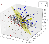
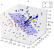
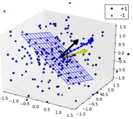
(a) (b) (c)
2.1 Model
Consider a dataset comprising i.i.d. pairs , . We refer to the vectors as features and to the binary variables as labels. We assume that the features are sampled from a Gaussian distribution with mean and a positive definite covariance . The labels are generated by a mixture of linear classifiers, i.e.,
| (2) |
Here, is the number of components in the mixture; are the weights, satisfying of course , ; and , are the normals to the planes defining the linear classifiers. We refer to each normal as the parameter profile of the -th classifier; we assume that the profiles , , are linearly independent, and that .
We assume that the function , characterizing the classifier response, is analytic, non-decreasing, strictly concave in , and satisfies:
| (3) |
As an example, it is useful to keep in mind the logistic function . Fig. 1(a) illustrates a mixture of classifiers over dimensions.
2.2 Subspace Estimation, Prediction and Clustering
Our main focus is the following task:
Subspace Estimation: After observing , estimate the subspace spanned by the profiles of the classifiers, i.e., .
For an estimate of , we characterize performance via the principal angle between the two spaces, namely
Notice that projecting the features on entails no loss of information w.r.t. (2). This can be exploited to improve the performance of several learning tasks through dimensionality reduction, by projecting the features to the estimate of the subspace . Two such tasks are:
Prediction: Given a new feature vector , predict the corresponding label .
Clustering: Given a new feature vector and label pair , identify the classifier that generated the label.
As we will see in Section 5, our subspace estimate can be used to significantly improve the performance of both prediction and clustering.
2.3 Technical Preliminary
We review here a few definitions used in our exposition. The sub-gaussian norm of a random variable is:
We say is sub-gaussian if . We say that a random vector is sub-gaussian if is sub-gaussian for any on the unit sphere .
3 Subspace Estimation
In this section, we present our algorithm for subspace estimation, which we refer to as SpectralMirror. Our main technical contribution, stated formally below, is that the output of SpectralMirror is a consistent estimator of the subspace as soon as , for a sufficiently large constant .
3.1 Spectral Mirror Algorithm
We begin by presenting our algorithm for estimating the subspace span . Our algorithm consists of three main steps. First, as pre-processing, we estimate the mean and covariance of the underlying features . Second, using these estimates, we identify a vector that concentrates near the convex cone spanned by the profiles . We use this vector to perform an operation we call mirroring: we ‘flip’ all labels lying in the negative halfspace determined by . Finally, we compute a weighted covariance matrix over all , where each point’s contribution is weighed by the mirrored labels: the eigenvectors of this matrix, appropriately transformed, yield the span .
These operations are summarized in Algorithm 1. We discuss each of the main steps in more detail below:
Pre-processing. (Lines 1–2) We split the dataset into two halves. Using the first half (i.e., all with , we construct estimates and of the feature mean and covariance, respectively. Standard Gaussian (i.e., ‘whitened’) versions of features can be constructed as .
Mirroring. (Lines 3–4) We compute the vector:
| (5) |
We refer to as the mirroring direction. In Section 4, we show that concentrates around its population () version . Crucially, lies in the interior of the convex cone spanned by the parameter profiles, i.e., , for some positive , (see Lemma 2 and Fig. 1(b)). Using this , we ‘mirror’ the labels in the second part of the dataset:
In words, equals for all in the positive half-space defined by the mirroring direction; instead, all labels for points in the negative half-space are flipped (i.e., ). This is illustrated in Figure 1(c).
Spectral Decomposition. (Lines 5–8) The mirrored labels are used to compute a weighted covariance matrix over whitened features as follows:
The spectrum of has a specific structure, that reveals the span . In particular, as we will see in Section 4, converges to a matrix that contains an eigenvalue with multiplicity ; crucially, the eigenvectors corresponding to the remaining eigenvalues, subject to the linear transform , span the subspace . As such, the final steps of the algorithm amount to discovering the eigenvalues that ‘stand out’ (i.e., are different from the eigenvalue with multiplicity ), and rotating the corresponding eigenvectors to obtain . More specifically, let be the eigenvalues and eigenvectors of . Recall that . The algorithm computes the median of all eigenvalues, and identifies the eigenvalues furthest from this median; these are the ‘outliers’. The corresponding eigenvectors, multiplied by , yield the subspace estimate .
The algorithm does not require knowledge of the classifier response function . Also, while we assume knowledge of , an eigenvalue/eigenvectors statistic (see, e.g., Zelnik-Manor and Perona (2004)) can be used to estimate , as the number of ‘outlier’ eigenvalues.
3.2 Main Result
Our main result states that SpectralMirror is a consistent estimator of the subspace spanned by . This is true for ‘most’ . Formally, we say that an event occurs for generic if adding an arbitrarily small random perturbation to , the event occurs with probability w.r.t. this perturbation.
Theorem 1.
Denote by the output of SpectralMirror, and let be the projector orthogonal to , given by (6). Then, for generic , as well as for , there exists such that, for all ,
Here is an absolute constant, and depends on , , and .
In other words, provides an accurate estimate of as soon as is significantly larger than . This holds for generic , but we also prove that it holds for the specific and important case where ; in fact, it also holds for all small-enough . Note that this does not guarantee that spans the direction ; nevertheless, as shown below, the latter is accurately estimated by (see Lemma 1) and can be added to the span, if necessary. Moreover, our experiments suggest this is rarely the case in practice, as indeed includes the direction (see Section 5).
4 Proof of Theorem 1
Recall that we denote by the population () version of . Let , for , and observe that Hence,
| (6) |
Then, the following concentration result holds:
Lemma 1.
There exist an absolute constant and that depend on such that:
The proof of Lemma 1 relies on a large deviation inequality for sub-Gaussian vectors, and is provided in Appendix B. Crucially, lies in the interior of the convex cone spanned by the parameter profiles:
Lemma 2.
for some , .
Proof.
From (6),
It thus suffices to show that , for some . Note that is normal with mean and variance . Since is analytic and non-decreasing, so is ; moreover, . This, and the fact that is non-constant, implies . On the other hand, from Stein’s identity (4), , as is bounded. Hence:
and the lemma follows. ∎
For and as in Lemma 2, define
Observe that is the expectation of the mirrored label at a point presuming that the mirroring direction is exactly . Let be the matrix:
Then concentrates around , as stated below.
Lemma 3.
Let , where the are defined as per Lemma 2 and is the smallest non-zero singular value of . Then for :
where an absolute constant, and depend on , , and .
The proof of Lemma 3 is in Appendix C. We again rely on large deviation bounds for sub-gaussian random variables; nevertheless, our proof diverges from standard arguments because , rather than , is used as a mirroring direction. Additional care is needed to ensure that (a) when is close enough to , its projection to lies in the interior of the convex cone spanned by the profiles, and (b) although may have a (vanishing) component outside the convex cone, the effect this has on is negligible, for large enough.
An immediate consequence of Lemma 2 is that reveals a direction in the span . The following lemma states that the eigenvectors of , subject to a rotation, yield the remaining directions:
Lemma 4.
Matrix has at most distinct eigenvalues. One eigenvalue, termed , has multiplicity . For generic , as well as for , the eigenvectors corresponding to the remaining eigenvalues , …, are such that
where is the projection orthogonal to .
Proof.
Note that
for , , and . Hence where
By a rotation invariance argument, can be written as
| (7) |
for some . To see this, let , and suppose first that
| (8) |
Since is whitened, its coordinates are independent. Thus, under (8), for all s.t. and for , for some . Thus , where is symmetric and 0 everywhere except perhaps on (the top left block). Since the profiles are linearly independent, so are and , by Lemma 2. Hence, matrices span all such , so (7) follows. Moreover, since is whitened, is rotation invariant and thus (7) extends beyond (8); indeed, if , , where a rotation matrix (i.e. ), then . Hence, as (8) holds for some orthonormal basis, (7) holds for all bases.
Let . Then
Let be the projector orthogonal to , i.e., Let . Lemma 2 and the linear independence of imply that , for all . Define where , . We will show below that for generic , as well as for , for all . This implies that . Indeed, where has rank by the linear independence of profiles. As is a projector orthogonal to a 1-dimensional space, has rank at least . On the other hand, , for , and where so . The latter also implies that , as , , and .
The above imply that has one eigenvalue of multiplicity , namely . Moreover, the eigenvectors corresponding to the remaining eigenvalues (or, the non-zero eigenvalues of ) are such that
The lemma thus follows by multiplying both sides of the above equality with , and using the fact that
It remains to show that , for all , when is generic or 0. Note that
| (9) | ||||
It thus suffices to show that . Lemma 2 implies that for some , hence
where and are independent Gaussians with mean 0, and , . Hence, where
where the normal p.d.f. Assume first that . By (3), is anti-symmetric, i.e., . Thus, i.e., is symmetric. Further, . The strict concavity of in implies that is decreasing in , and the anti-symmetry of implies that is symmetric. Take : if , , while if , then , so is negative for . By the symmetry of , is positive for . As such, for some strictly decreasing , and for ; hence, , for all .
To see that for generic , recall that is analytic and hence so is . Hence, is an analytic function of , for every ; also, as for , it is not identically 0. Hence, the sets , , have Lebesgue measure 0 (see, e.g., pg. 83 in (analytic)), and so does their union . As such, for generic ; if not, there exists a ball such that has positive Lebesgue measure, a contradiction. ∎
(a) vs. (b) vs.
(a) (b)
Denote by the eigenvalue of multiplicity in Lemma 4. Let be the gap between and the remaining eigenvalues. Then, the following lemma holds; this, along with Lemma 4, yields Theorem 1.
Lemma 5.
Let be our estimate for . If are separated from by at least , then for , we have
where , are defined as per Lemma 3.
Proof.
If we ensure , then, by Weyl’s theorem (Horn and Johnson, 2012), eigenvalues of are contained in , and the remaining eigenvalues are outside this set, and will be detected by SpectralMirror. Moreover, by the Davis-Kahan theorem,
Thus the event is implied by Moreover, this implies that sufficient condition for (which is required for SpectralMirror to detect the correct eigenvalues) is that . The lemma thus follows from Lemma 3. ∎
Note that the Gaussianity of is crucially used in the fact that the ‘whitened’ features are uncorrelated, which in turn yields Eq. (7). We believe that the theorem can be extended to more general distributions, provided that the transform de-correlates the coordinates of .
5 Experiments
(a) EM Prediction (close to gr. truth) (b) EM Prediction (random) (c) Clustering (random)
We conduct computational experiments to validate the performance of SpecralMirror on subspace estimation, prediction, and clustering. We generate synthetic data using , with profiles and mixture weights sampled uniformly at random from the -dimensional simplex. Features are also Gaussian: ; labels generated by the -th classifier are given by .
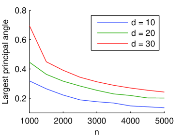
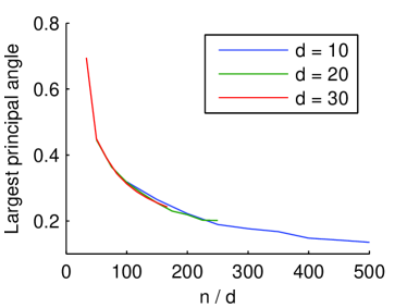
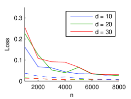
Convergence. We study first how well SpectralMirror estimates the span . Figure 2(a) shows the convergence of to in terms of (the sin of) the largest principal angle between the subspaces versus the sample size . We also plot the convergence versus the effective sample size (Figure 2(a)). The curves for different values of align in Figure 2, indicating that the upper bound in Thm. 1 correctly predicts the sample complexity as . Though not guaranteed by Theorem 1, in all experiments was indeed spanned by , so the addition of to was not necessary.
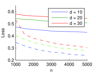
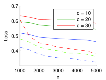
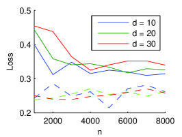
Prediction through -NN. Next, we use the estimated subspace to aid in the prediction of expected labels. Given a new feature vector , we use the average label of its nearest neighbors (-NN) in the training set to predict its expected label. We do this for two settings: once over the raw data (the ‘ambient’ space), and once over data for which the features are first projected to , the estimated span (of dimension 2). For each , we repeat this procedure 25 times with and . We record the average root mean squared error between predicted and expected labels over the 25 runs. Figures 3(a) and 3(b) show that, despite the error in , using -NN on this subspace outperforms -NN on the ambient space.
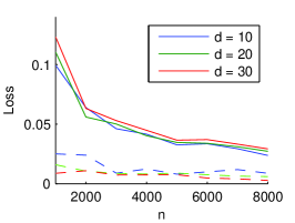
Prediction and Clustering through EM. We next study the performance of prediction and clustering using the Expectation-Maximization (EM) algorithm. We use EM to fit the individual profiles both over the training set, as well as on the dataset projected to the estimated subspace . We conducted two experiments in this setting: (a) initialize EM close to the true profiles , , and (b) randomly initialize EM and choose the best set of profiles from 30 runs. For each we run EM 10 times.
The first set of prediction experiments, we again compare expected labels to the predicted labels, using for the latter profiles and mixture probabilities as estimated by EM. Figure 4(a) measures the statistical efficiency of EM over the estimated subspace versus EM over the ambient space, when EM is initialized close to the true profiles. The second set of experiments, illustrated in Figure 4(b), aims to capture the additional improvement due to the reduction in the number of local minima in the reduced space. In both cases we see that constraining the estimated profiles to lie in the estimated subspace improves the statistical efficiency of EM; in the more realistic random start experiments, enforcing the subspace constraint also improves the performance of EM by reducing the number of local minima. We also observe an overall improvement compared to prediction through -NN.
Finally, we use the fitted profiles to identify the classifier generating a label given the features and the label. To do this, once the profiles have been detected by EM, we use a logistic model margin condition to identify the classifier who generated a label, given the label and its features. Figure 4(c) shows the result for EM initialized at a random point, after choosing the best set of profiles from out of 30 runs. We evaluate the performance of this clustering procedure using the normalized 0-1 loss. Again, constraining the estimated profiles to the estimated subspace significantly improves the performance of this clustering task.
6 Conclusions
We have proposed SpectralMirror, a method for discovering the span of a mixture of linear classifiers. Our method relies on a non-linear transform of the labels, which we refer to as ‘mirroring’. Moreover, we have provided consistency guarantees and non-asymptotic bounds, that also imply the near optimal statistical efficiency of the method. Finally, we have shown that, despite the fact that SpectralMirror discovers the span only approximately, this is sufficient to allow for a significant improvement in both prediction and clustering, when the features are projected to the estimated span.
We have already discussed several technical issues that remain open, and that we believe are amenable to further analysis. These include amending the Gaussianity assumption, and applying our bounds to other pHd-inspired methods. An additional research topic is to further improve the computational complexity of the estimation of the eigenvectors of the ‘mirrored’ matrix . This is of greatest interest in cases where the covariance and mean are a priori known. This would be the case when, e.g., the method is applied repeatedly and, although the features are sampled from the same distribution each time, labels are generated from a different mixture of classifiers. In this case, SpectralMirror lacks the pre-processing step, that requires estimating and is thus computationally intensive; the remaining operations amount to discovering the spectrum of , an operation that can be performed more efficiently. For example, we can use a regularized M-estimator to exploit the fact that should be the sum of a multiple of the identity and a low rank matrix—see, e.g., Negahban et al. (2012).
References
- Anandkumar et al. (2012) {barticle}[author] \bauthor\bsnmAnandkumar, \bfnmAnima\binitsA., \bauthor\bsnmGe, \bfnmRong\binitsR., \bauthor\bsnmHsu, \bfnmDaniel\binitsD., \bauthor\bsnmKakade, \bfnmSham M\binitsS. M. and \bauthor\bsnmTelgarsky, \bfnmMatus\binitsM. (\byear2012). \btitleTensor decompositions for learning latent variable models. \bjournalarXiv preprint arXiv:1210.7559. \endbibitem
- Arora and Kannan (2001) {binproceedings}[author] \bauthor\bsnmArora, \bfnmSanjeev\binitsS. and \bauthor\bsnmKannan, \bfnmRavi\binitsR. (\byear2001). \btitleLearning mixtures of arbitrary gaussians. In \bbooktitleProceedings of the thirty-third annual ACM symposium on Theory of computing \bpages247–257. \bpublisherACM. \endbibitem
- Bartholomew, Knott and Moustaki (2011) {bbook}[author] \bauthor\bsnmBartholomew, \bfnmDavid J\binitsD. J., \bauthor\bsnmKnott, \bfnmMartin\binitsM. and \bauthor\bsnmMoustaki, \bfnmIrini\binitsI. (\byear2011). \btitleLatent variable models and factor analysis: A unified approach \bvolume899. \bpublisherWiley. com. \endbibitem
- Bishop (1998) {bincollection}[author] \bauthor\bsnmBishop, \bfnmChristopher M\binitsC. M. (\byear1998). \btitleLatent variable models. In \bbooktitleLearning in graphical models \bpages371–403. \bpublisherSpringer. \endbibitem
- Chaganty and Liang (2013) {binproceedings}[author] \bauthor\bsnmChaganty, \bfnmArun Tejasvi\binitsA. T. and \bauthor\bsnmLiang, \bfnmPercy\binitsP. (\byear2013). \btitleSpectral experts for estimating mixtures of linear regressions. In \bbooktitleICML. \endbibitem
- Cook (1998) {barticle}[author] \bauthor\bsnmCook, \bfnmR Dennis\binitsR. D. (\byear1998). \btitlePrincipal Hessian directions revisited. \bjournalJournal of the American Statistical Association \bvolume93 \bpages84–94. \endbibitem
- Dempster, Laird and Rubin (1977) {barticle}[author] \bauthor\bsnmDempster, \bfnmArthur P\binitsA. P., \bauthor\bsnmLaird, \bfnmNan M\binitsN. M. and \bauthor\bsnmRubin, \bfnmDonald B\binitsD. B. (\byear1977). \btitleMaximum likelihood from incomplete data via the EM algorithm. \bjournalJournal of the Royal Statistical Society. Series B (Methodological) \bpages1–38. \endbibitem
- Horn and Johnson (2012) {bbook}[author] \bauthor\bsnmHorn, \bfnmRoger A\binitsR. A. and \bauthor\bsnmJohnson, \bfnmCharles R\binitsC. R. (\byear2012). \btitleMatrix analysis. \bpublisherCambridge university press. \endbibitem
- Hsu, Kakade and Zhang (2012) {barticle}[author] \bauthor\bsnmHsu, \bfnmDaniel\binitsD., \bauthor\bsnmKakade, \bfnmSham M\binitsS. M. and \bauthor\bsnmZhang, \bfnmTong\binitsT. (\byear2012). \btitleA spectral algorithm for learning hidden Markov models. \bjournalJournal of Computer and System Sciences \bvolume78 \bpages1460–1480. \endbibitem
- Jordan and Jacobs (1994) {barticle}[author] \bauthor\bsnmJordan, \bfnmMichael I\binitsM. I. and \bauthor\bsnmJacobs, \bfnmRobert A\binitsR. A. (\byear1994). \btitleHierarchical mixtures of experts and the EM algorithm. \bjournalNeural computation \bvolume6 \bpages181–214. \endbibitem
- Li (1992) {barticle}[author] \bauthor\bsnmLi, \bfnmKer-Chau\binitsK.-C. (\byear1992). \btitleOn principal Hessian directions for data visualization and dimension reduction: another application of Stein’s lemma. \bjournalJournal of the American Statistical Association \bvolume87 \bpages1025–1039. \endbibitem
- Liang et al. (2006) {binproceedings}[author] \bauthor\bsnmLiang, \bfnmPercy\binitsP., \bauthor\bsnmBouchard-Côté, \bfnmAlexandre\binitsA., \bauthor\bsnmKlein, \bfnmDan\binitsD. and \bauthor\bsnmTaskar, \bfnmBen\binitsB. (\byear2006). \btitleAn end-to-end discriminative approach to machine translation. In \bbooktitleProceedings of the 21st International Conference on Computational Linguistics and the 44th annual meeting of the Association for Computational Linguistics \bpages761–768. \bpublisherAssociation for Computational Linguistics. \endbibitem
- Liu (1994) {barticle}[author] \bauthor\bsnmLiu, \bfnmJun S\binitsJ. S. (\byear1994). \btitleSiegel’s formula via Stein’s identities. \bjournalStatistics & Probability Letters \bvolume21 \bpages247–251. \endbibitem
- McLachlan and Peel (2004) {bbook}[author] \bauthor\bsnmMcLachlan, \bfnmGeoffrey\binitsG. and \bauthor\bsnmPeel, \bfnmDavid\binitsD. (\byear2004). \btitleFinite mixture models. \bpublisherWiley. com. \endbibitem
- Moitra and Valiant (2010) {binproceedings}[author] \bauthor\bsnmMoitra, \bfnmAnkur\binitsA. and \bauthor\bsnmValiant, \bfnmGregory\binitsG. (\byear2010). \btitleSettling the polynomial learnability of mixtures of gaussians. In \bbooktitleFoundations of Computer Science (FOCS), 2010 51st Annual IEEE Symposium on \bpages93–102. \bpublisherIEEE. \endbibitem
- Negahban et al. (2012) {barticle}[author] \bauthor\bsnmNegahban, \bfnmSahand N\binitsS. N., \bauthor\bsnmRavikumar, \bfnmPradeep\binitsP., \bauthor\bsnmWainwright, \bfnmMartin J\binitsM. J. and \bauthor\bsnmYu, \bfnmBin\binitsB. (\byear2012). \btitleA unified framework for high-dimensional analysis of -estimators with decomposable regularizers. \bjournalStatistical Science \bvolume27 \bpages538–557. \endbibitem
- Pearson (1894) {barticle}[author] \bauthor\bsnmPearson, \bfnmKarl\binitsK. (\byear1894). \btitleContributions to the mathematical theory of evolution. \bjournalPhilosophical Transactions of the Royal Society of London. A \bvolume185 \bpages71–110. \endbibitem
- Quattoni, Collins and Darrell (2004) {binproceedings}[author] \bauthor\bsnmQuattoni, \bfnmAriadna\binitsA., \bauthor\bsnmCollins, \bfnmMichael\binitsM. and \bauthor\bsnmDarrell, \bfnmTrevor\binitsT. (\byear2004). \btitleConditional random fields for object recognition. In \bbooktitleAdvances in neural information processing systems \bpages1097–1104. \endbibitem
- Stein (1973) {binproceedings}[author] \bauthor\bsnmStein, \bfnmCharles M\binitsC. M. (\byear1973). \btitleEstimation of the mean of a multivariate normal distribution. In \bbooktitlePrague Symposium on Asymptotic Statistics. \endbibitem
- Vershynin (2010) {barticle}[author] \bauthor\bsnmVershynin, \bfnmR.\binitsR. (\byear2010). \btitleIntroduction to the non-asymptotic analysis of random matrices. \bjournalarXiv preprint arXiv:1011.3027. \endbibitem
- Zelnik-Manor and Perona (2004) {binproceedings}[author] \bauthor\bsnmZelnik-Manor, \bfnmLihi\binitsL. and \bauthor\bsnmPerona, \bfnmPietro\binitsP. (\byear2004). \btitleSelf-tuning spectral clustering. In \bbooktitleAdvances in neural information processing systems \bpages1601–1608. \endbibitem
Appendix A A Large-Deviation Lemma
We first prove a Bernstein-type inequality for sub-Gaussian random vectors, that we shall use in our proofs:
Lemma 6.
Let be a sub-Gaussian random vector, i.e. is sub-Gaussian for any . Then there exist universal constants such that
Proof.
By the (exponential) Markov inequality, we have
| (10) |
Let be uniformly distributed on the unit sphere . Then is isotropic so for all . We use this fact to bound the m.g.f. of :
We interchange the order of expectation to obtain
is sub-Gaussian (for fixed ) so is (noncentered) sub-exponential. If , then
| (11) |
We substitute this bound into (10) to obtain
where is the covariance matrix of . We optimize over to obtain
If the optimum lies outside the region where the m.g.f. bound holds (11), we can always choose
in to obtain the tail bound:
We combine these two bounds to obtain
Note that the bound always holds. However, for small , the term yields a tighter bound. ∎
Appendix B Proof of Lemma 1 (Weak Conv. of )
Proof.
We expand (and neglect higher order terms) to obtain
| (12) |
The higher order terms generically look like
| (13) |
We apply the union bound to deduce
For any , and we have
Since terms of the form appear in the upper bounds we derive, we can handle terms like (13) with a constant factor (say 2). Since our bounds involve multiplicative constant factors anyways, we neglect these terms to simplify our derivation.
We expand the first term to obtain
is a sub-Gaussian random variable with sub-Gaussian norm , so there exist universal and s.t.
is bounded between 1 and -1, so
-
1.
We can use Chernoff’s inequality to deduce
-
2.
are sub-Gaussian. Thus there exist universal and such that
We expand the second term in (12) to obtain
We expand the middle term to obtain
We use Theorem 5.39 in Vershynin (2010) to bound the first term:
where depend on the sub-Gaussian norm of . We substitute these bounds into our expression for to deduce
where is an absolute constant and depend on the sub-Gaussian norm of . ∎
Appendix C Proof of Lemma 3 (Weak Conv. of )
Let denote the projection of onto .
Lemma 7.
If
then lies in the interior of the positive cone spanned by , where is the smallest nonzero singular value of .
Proof.
lies in interior of the conic hull of , so we can express as , where . If also lies in the conic hull, then for some . Then
To ensure is component-wise positive, we must have . A sufficient condition is . ∎
We are now ready to prove Lemma 3. We expand (and neglect higher order terms) to obtain
The second and third terms can be bounded using the same bounds used in the analysis of how fast converges to . Thus we focus on how fast
coverges to . Let . First, we note that
| (14) | |||
Let denote the “corrected” version of the ’s, i.e. the ’s we obtain if we use the projection of onto to flip the labels, and denote . We have
| (15) | ||||
The probability the first term is large is bounded by
| (16) | |||
The ’s are independent of ’s because the ’s were computed using that was in turn computed independently of the ’s, as the former are computed on a different partition of . Thus, the sum in the r.h.s. of (15) is a sum of i.i.d. r.v. and can be bounded by
where depend on the sub-Gaussian norm of . This is a consequence of Remark 5.40 in Vershynin (2010).
We now focus on bounding the second term in (15). In what follows, without loss of generality, we will restrict to the k+1 subspace spanned by and , as remaining components of the ’s do not contribute to the computation. Let (for cone) be the “bad” region, i.e. the region where . We have
By the triangle inequality, we have
| (17) | ||||
is bounded, hence is sub-Gaussian and
| (18) |
where depend on the sub-Gaussian norm of . It remains to bound .
We use Jensen’s inequality to obtain
| (19) |
where the constant depends on , as is restricted to the space spanned by and . Finally, we bound .
The distribution of is spherically symmetric so the probability that is proportional to the surface area of the set , where the unit sphere centered at the origin:
Lemma 2 implies that this set is contained in the set
By a symmetry argument, the volume of (according to the normalized measure on the unit sphere) is simply the angle between and , i.e.
Let . Recall that , by conditioning; it can be verified that this implies . Thus
where depends on . We substitute these bounds into (19) to obtain
| (20) |
We combine (20) with (18) to deduce
Using this expression and (16), a union bound on Ineq. (15) gives:
| (21) |
for appropriate constants ,,,. Note that
Let
The first term is bounded by and the second term is bounded by . We deduce
To complete the proof of Lemma 3, one can similarly account for the event in (14), finaly yielding:
The lemma thus follows from the fact that for small enough .
Appendix D Principal Hessian Directions
In this section, we apply the principal Hessian directions (pHd) (Li, 1992) method to our setting, and demontrate its failure to discover the space spanned by parameter profile when . Recall that pHd considers a setting in which features are i.i.d. and normally distributed with mean and covariance , while labels lie, in expectation, in a -dimensional manifold. In particular, some smooth , :
where , . The method effectively creates an estimate
of the Hessian
| (22) | ||||
where is the Hessian of the mapping , for , and the matrix of profiles. As in our case, the method discovers from the eigenvectors of the eigenvalues that “stand out”, after appropriate rotation in terms of .
Unfortunately, in the case of linear classifiers,
for is anti-symmetric. As a result, is a diagonal matrix whose -th entry in the diagonal is . Since is anti-symmetric, so is . Hence, if we have that ; hence, the Hessian given by (22) will in fact be zero, and the method will fail to discover any signal pertaining to .
This calls for an application of the pHd method to a transform of the labels . This ought to be non-linear, as an affine transform would preserve the above property. Moreover, given that these labels are binary, polynomial transforms do not add any additional signal to , and are therefore not much help in accomplishing this task. In contrast, the ‘mirrorring’ approach that we propose provides a means of transforming the labels so that their expectation indeed carries sufficient information to extract the span , as evidenced by Theorem 1.