QCD analysis of polarized DIS and the SIDIS asymmetry world data and light sea-quark decomposition

Abstract

The results of our new QCD analysis of helicity parton distributions of the nucleon at full next-to-leading order (NLO) accuracy in the fixed-flavor number scheme will be presented. Performing a combined QCD fit on the global sets of latest inclusive and the semi-inclusive polarized deep inelastic scattering data, we are able to extract new polarized parton distribution functions (PPDFs) at the input scale $Q_{0}^{2}=1$ GeV². Particulary, we have calculated PPDFs considering light sea-quark decomposition and the results are compared with the experimental data and the most precise theoretical models obtained by recent analyses. The latest COMPASS2010 SIDIS data, which were not available for the previous analyses, are employed in the current analysis and the effect of COMPASS SIDIS data is studied in detail. Also the uncertainties of PPDFs are determined using the standard Hessian technique.

I Introduction

In the recent years the determination of nucleon partonic composition and their spin projections from high energy experimental data has improved remarkably and the extracted polarized and unpolarized partonic distributions have very essential role in the study of hard scattering processes phenomenology. For the case of polarized parton distributions, the experimental discoveries of nucleon spin in the late 1980’s EMC1 ; EMC2 proved the spin contribution of valence quarks is anomalously small and the predictions are far from reality, then the theoretical assumptions on perturbative QCD were applied to interpret theses experimental results Anselmino:1994gn ; Lampe:1998eu ; Hughes:1999wr ; filippone-01 ; Altarelli:2009za .

In the recent decades the determination of PPDFs and their uncertainties from deep inelastic scattering (DIS) experiments performing at CERN, SLAC, DESY and JLAB EMCp ; SMCpd ; COMP1 ; E142n ; E143pd ; E154n ; E155d ; E155p ; hermespdf ; HERMn ; HERMpd ; JLabn ; CLA1pd spread very fast Ball:2013lla ; Gehrmannn ; Blumlein:2010rn ; PRD11 ; lea99 ; Ball:1997sp ; bou98 ; gor98 ; alt98abfr ; str99 ; gho00 ; Gluck:2000dy ; Bhalerao:2001rn ; Leader:2001kh ; Bluemlein:2002be ; Goto:1999by ; Leader:2005ci ; Bourrely:2001du ; ABFR ; alt97 ; Hirai:2008aj ; Khorramian:2004ih ; AtashbarTehrani:2007be ; AtashbarTehrani:2011zz ; Arbabifar:2011zz ; Khorramian:2010zz and recently semi inclusive deep inelastic scattering (SIDIS) experimental data SMC98 ; hermespdf ; COMP1_h ; COMP1_pK have been also included by some of the theoretical groups lss ; dns ; deFlorian:2000bm ; deFlorian:2005mw ; deFlorian:2008mr . The only theoretical group which perform a combined NLO analysis of DIS, SIDIS and polarized proton proton collision data was DSSV in 2008 deFlorian:2009vb . The extracted PPDFs of valence quarks lightly differ but the PPDFs of sea quarks and gluon are more different caused by datasets selection, parametrization forms of PPDFs and the method of evolution and QCD analysis. The effect of different PPDFs and the spin Physics on the determination of fragmentation functions have been studied recently in Ref. Soleymaninia:2013cxa

In our latest analysis we studied the impact of inclusive DIS data on the determination of PPDFs based on Jacobi polynomials with flavor symmetric light sea distribution, i.e. $\delta\bar{u}=\delta\bar{d}=\delta\bar{s}=\delta s$ PRD11 , and now we consider light sea-quark decomposition and include additional SIDIS data SMC98 ; hermespdf ; COMP1_h ; COMP1_pK ; compass10 . In fact, fully inclusive DIS data from many different experiments are just impressive to determine the sum of the quark and anti-quark distributions while SIDIS data help to tell difference between quarks and anti-quarks as well. Here we focus on the effect of SIDIS data on determination of PPDFs, specially sea quarks distribution separation which was not considered in our last DIS data analysis and we present the comparison between both results. The impact of RHIC polarized proton proton collision data will be studied in a separate publication in near future.

In the present analysis we utilize the full sets of proton and deuteron SIDIS asymmetry data from the COMPASS group at CERN COMP1_h ; COMP1_pK ; compass10 which were partially considered by the last analysis on SIDIS data deFlorian:2009vb ; lss . Specially we use the new semi inclusive asymmetries COMPASS2010 proton data for charged pions and kaons production from polarized proton target, $A_{1}^{p,\pi^{\pm}}$ and $A_{1}^{p,k^{\pm}}$ compass10 , which were not available for the analysis before 2010 and are helpful to study $\delta s$ and $\delta\bar{s}$ distributions due to kaon detection from polarized proton for the first time compass10 . In order to discuss more about the effect of COMPASS SIDIS data on polarized $\bar{u}$, $\bar{d}$ and $s=\bar{s}$ we perform extra analysis excluding these datasets. The comparison of results shows the effect of their inclusion clearly.

The current study presents a new NLO QCD analysis of the polarized DIS and SIDIS data and we extract new parametrization forms of PPDFs in flavor SU(2) and SU(3) symmetry breaking. Here we also propose a simplified form of double Mellin convolution expressions which saves times during fitting procedure. Also the behavior of $\Delta\chi^{2}$ and the uncertainty of PPDFs are calculated using the standard Hessian method.

This paper is organized as follows. In Sec. II we present the relationship between polarized structure functions and asymmetry data as observables and then we review the datasets used in our analysis on PPDFs. QCD analysis including parametrization, evolution and simplification of double Mellin convolution of PPDFs, Wilson coefficients and FFs are discussed in Sec. III. Sec. IV presents the fitting procedure and global $\chi^{2}$ minimization for asymmetry data and the investigation of $\chi^{2}$ neighborhood and error calculation by standard Hessian method. We present the full results of our fit to the data, comparison with other models and sum rules in Sec. V and finally Sec. VI contains the summary of the whole work.

II Experimental observables and datasets

II.1 Polarized asymmetries

Perturbative QCD can predict polarized structure function $g_{1}(x,Q^{2})$ in terms of PPDFs and strong coupling constant up to NLO approximation. However, experimental groups measure cross section asymmetries $A_{\parallel}$ and $A_{\bot}$ defined by the following ratios

$$A_{\parallel} = \frac{d\sigma^{\rightarrow\Rightarrow}-d\sigma^{\rightarrow\Leftarrow}}{d\sigma^{\rightarrow\Rightarrow}+d\sigma^{\rightarrow\Leftarrow}}~{},$$

$$A_{\bot} = \frac{d\sigma^{\rightarrow\Uparrow}-d\sigma^{\rightarrow\Downarrow}}{d\sigma^{\rightarrow\Uparrow}+d\sigma^{\rightarrow\Downarrow}}~{},$$ (1)

where $d\sigma^{\rightarrow\Rightarrow}$ and $d\sigma^{\rightarrow\Leftarrow}$ are cross sections for longitudinal polarized lepton scattering of a parallel or anti-parallel polarized target hadron, and $d\sigma^{\rightarrow\Uparrow}$ and $d\sigma^{\rightarrow\Downarrow}$ are the same for a transversely polarized hadron.

The ratio of polarized and unpolarized structure functions, $g_{1}$ and $F_{1}$, is related to the measurable asymmetries by

$$\frac{g_{1}(x,Q^{2})}{F_{1}(x,Q^{2})} = \frac{1}{(1+\gamma^{2})(1+\eta\zeta)}$$ (2)

$$\left[(1+\gamma\zeta)\frac{A_{\parallel}}{D}-(\eta-\gamma)\frac{A_{\bot}}{d}\right]~{},$$

and the definitions of kinematic factors are given by

$$\gamma = \frac{2Mx}{\sqrt{Q^{2}}}~{},$$ (3)

$$d = \frac{D\sqrt{1-y-\gamma^{2}y^{2}/4}}{1-y/2}~{},$$ (4)

$$D = \frac{1-(1-y)\epsilon}{1+\epsilon R(x,Q^{2})}~{},$$ (5)

$$\eta = \frac{\epsilon\gamma y}{1-\epsilon(1-y)}~{},$$ (6)

$$\zeta = \frac{\gamma(1-y/2)}{1+\gamma^{2}y/2}~{},$$ (7)

$$\epsilon = \frac{4(1-y)-\gamma^{2}y^{2}}{2y^{2}+4(1-y)+\gamma^{2}y^{2}}~{},$$ (8)

here $M$ denotes the nucleon mass and $y=(E-E^{\prime})/E$ describes the normalized energy fraction transferred to the virtual photon, with $E$ the energy of incoming lepton and $E^{\prime}$ the energy of scattered lepton in the nucleon rest frame. The unpolarized structure function $F_{1}$ is expressed by its expression in terms of measured unpolarized structure function $F_{2}$ extracted from unpolarized DIS experiments NMC

$$F_{1}(x,Q^{2})=\frac{(1+\gamma^{2})}{2x(1+R(x,Q^{2}))}F_{2}(x,Q^{2})~{},$$ (9)

and $R$ is the ratio of longitudinal to transverse photon-nucleon unpolarized structure function which is determined in Ref. R1998

$$R(x,Q^{2})=\frac{F_{L}(x,Q^{2})}{F_{2}(x,Q^{2})-F_{L}(x,Q^{2})}~{}.$$ (10)

The asymmetries $A_{\parallel}$ and $A_{\bot}$ can be expressed in terms of $A_{1}$ and $A_{2}$, which are the virtual-photon longitudinal and transverse asymmetries, by

$$A_{\parallel} = D(A_{1}+\eta A_{2})~{},$$

$$A_{\bot} = d(A_{2}-\zeta A_{1})~{},$$ (11)

where

$$A_{1}(x,Q^{2}) = \frac{\sigma_{1/2}^{T}-\sigma_{3/2}^{T}}{\sigma_{1/2}^{T}+\sigma_{3/2}^{T}}~{},$$

$$A_{2}(x,Q^{2}) = \frac{2\sigma^{TL}}{\sigma_{1/2}^{T}+\sigma_{3/2}^{T}}~{}.$$ (12)

Note that $\sigma_{1/2}^{T}$ and $\sigma_{3/2}^{T}$ recall the virtual transversly polarized photon scattering cross sections when the total spin of photon-nucleon system is $1/2$ or $3/2$ respectively, and $\sigma^{TL}$ is the term denoting the interference of longitudinal and transverse photon-nucleon amplitudes. Finally using Eqs. 11 and 2 one can find the relation between polarized and unpolarized structure functions $g_{1}$ and $F_{1}$, and the asymetries $A_{1}$ and $A_{2}$ Bass:2004xa

$$\frac{g_{1}}{F_{1}}=\frac{1}{1+\gamma^{2}}[A_{1}+\gamma A_{2}]~{}.$$ (13)

The value of $A_{2}$ has been determined by SMC SMCR , E154 E154R and E143 E143R and the measurements showed its contribution to $g_{1}/F_{1}$ can be neglected in a good approximation, also it is being suppressed by the small value of kinematic factor $\gamma$ in the limit $m^{2}\ll Q^{2}$.

In our QCD analysis we perform fit procedure on $A_{1}$ or $g_{1}/F_{1}$ for DIS data

$$A_{1}(x,Q^{2})=\frac{g_{1}(x,Q^{2})}{F_{1}(x,Q^{2})}(1+\gamma^{2})~{}.$$ (14)

Note that such a procedure is equivalent to a fit to $(g_{1})_{exp}$, but it is more precise than the fit to the $g_{1}$ data themselves presented by the experimental groups because here the $g_{1}$ data are extracted in the same way for all of the datasets.

Unlike the inclusive polarized deep inelastic scattering wherein $g_{1}$ structure function is measured by detecting only the final state lepton, the particle detected in semi inclusive polarized deep inelastic experiments are charged hadrons in addition to scattered lepton. When the energy fraction of hadron, $z=E_{h}/E_{\gamma}$ is large, the most possible occurrence of detected hadrons are $\pi^{\pm}$ and $k^{\pm}$ which include struck quarks in their valance state. The double-spin asymmetry in SIDIS experiments for the production of hadron $h$ is

$$A_{1N}^{h}(x,z,Q^{2})=\frac{g_{1N}^{h}(x,z,Q^{2})}{F_{1N}^{h}(x,z,Q^{2})}~{}.$$ (15)

The structure functions $g_{1}^{h}$ and $F_{1}^{h}$ are fully determined in terms of polarized and unpolarized distributions respectively up to NLO approximation and will be discussed in Sec III. Thus we will determine $g_{1}$ and $g_{1N}^{h}$ from Eqs. 14 and 15 in the analysis and extract polarized parton distribution functions.

II.2 The datasets and ranges

We utilize two types of datasets from DIS and SIDIS experiments which come from relevant experiments done at DESY, SLAC, JLAB and CERN. The datasets used in our QCD analysis are summarized in Table 1. These experiments have different targets, including protons, neutrons and deuterons, and also different detected hadrons, including $\pi^{\pm}$, $k^{\pm}$ and $h^{\pm}$, for SIDIS reactions. We also show the number of data and the kinematic cuts on the experiments in Table 1, we exclude the data points which are in the range of $Q^{2}<1$ from our analysis, since below $Q^{2}=1$ GeV² perturbative QCD is not reliable. The summary of observables is as follows:
$\bullet$ EMCp, SMCpd, COMPASS, E142, E143, E154, E155 HERMES and JLAB DIS data
These experiments all determined $A_{1}$ except of E155 E155p ; E155d and HERMES HERMn which present $g_{1}/F_{1}$ and JLAB JLabn present both measurements. Since we consider different masses of nucleons in $\gamma$ in Eq. 14, we distinguish these two data types.

$\bullet$ SMCpd, HERMES and COMPASS SIDIS data
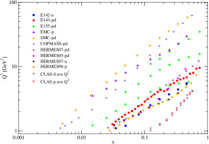
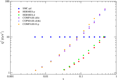
These experiments measure $A_{1N}^{h}$ as in Eq. 15 from semi inclusive reactions. The very recent and precise proton data of COMPASS compass10 are used for the first time in the current analysis. Figs 1 and 2 shows the DIS and SIDIS used data points in a scatter plot, as can been seen the region of $x$ and $Q^{2}$ is restricted to $0.004\lesssim x\lesssim 0.75$ and $1.0\lesssim Q^{2}\lesssim 60$ GeV² for DIS and $0.005\lesssim x\lesssim 0.5$ and $1.0\lesssim Q^{2}\lesssim 60$ GeV² for SIDIS experiments. We try to use all available data for DIS and SIDIS experiments to cover a large range of kinematics variables in comparison to other recent analysis Blumlein:2010rn ; lss ; deFlorian:2009vb .

Experiment	Process	$N_{data}$	$x_{min}$	$x_{max}$	$Q_{min}^{2}$ [GeV2]	$Q_{max}^{2}$ [GeV2]	$F$	$\chi^{2}$
EMC EMCp	DIS(p)	10	0.015	0.466	3.5	29.5	$A_{1}^{p}$	3.9
SMC SMCpd	DIS(p)	12	0.005	0.48	1.3	58	$A_{1}^{p}$	3.4
SMC SMCpd	DIS(d)	12	0.005	0.479	1.3	54.8	$A_{1}^{d}$	17.1
COMPASS COMP1	DIS(p)	15	0.0046	0.568	1.1	62.1	$A_{1}^{p}$	20.5
COMPASS COMP1	DIS(d)	15	0.0046	0.566	1.1	55.3	$A_{1}^{d}$	13.6
SLAC/E142 E142n	DIS(n)	8	0.035	0.466	1.1	5.5	$A_{1}^{n}$	4.18
SLAC/E143 E143pd	DIS(p)	28	0.031	0.749	1.27	9.52	$A_{1}^{p}$	22.0
SLAC/E143 E143pd	DIS(d)	28	0.031	0.749	1.27	9.52	$A_{1}^{d}$	54.6
SLAC/E154 E154n	DIS(n)	11	0.017	0.564	1.2	15	$A_{1}^{n}$	3.3
SLAC/E155 E155p	DIS(p)	24	0.015	0.75	1.22	34.72	$\frac{g_{1}^{p}}{F_{1}^{p}}$	22.5
SLAC/E155 E155d	DIS(d)	24	0.015	0.75	1.22	34.72	$\frac{g_{1}^{d}}{F_{1}^{d}}$	21.4
HERMES hermespdf	DIS(p)	9	0.033	0.447	1.22	9.18	$A_{1}^{p}$	4.5
HERMES hermespdf	DIS(d)	9	0.033	0.447	1.22	9.16	$A_{1}^{d}$	11.4
HERMES HERMn	DIS(n)	9	0.033	0.464	1.22	5.25	$A_{1}^{n}$	2.5
HERMES HERMn	DIS(p)	19	0.028	0.66	1.01	7.36	$\frac{g_{1}^{p}}{F_{1}^{p}}$	21.4
HERMES HERMpd	DIS(p)	15	0.0264	0.7248	1.12	12.21	$A_{1}^{p}$	10.2
HERMES HERMpd	DIS(d)	15	0.0264	0.7248	1.12	12.21	$A_{1}^{d}$	16.7
JLab-Hall A JLabn	DIS(n)	3	0.33	0.6	2.71	4.38	$\frac{g_{1}^{n}}{F_{1}^{n}}$	0.8
CLAS CLA1pd	DIS(p)	151	0.1088	0.5916	1.01	4.96	$A_{1}^{p}$	151.0
CLAS CLA1pd	DIS(d)	482	0.1366	0.57	1.01	4.16	$A_{1}^{d}$	442.5
SMC SMC98	SIDIS(p,$h^{+}$)	12	0.005	0.48	10	10	$A_{1}^{p,h^{+}}$	23.0
SMC SMC98	SIDIS(p,$h^{-}$)	12	0.005	0.48	10	10	$A_{1}^{p,h^{-}}$	11.9
SMC SMC98	SIDIS(d,$h^{+}$)	12	0.005	0.48	10	10	$A_{1}^{d,h^{+}}$	6.3
SMC SMC98	SIDIS(d,$h^{-}$)	12	0.005	0.48	10	10	$A_{1}^{d,h^{-}}$	17.2
HERMES hermespdf	SIDIS(p,$h^{+}$)	9	0.034	0.448	1.21	9.76	$A_{1}^{p,h^{+}}$	15.0
HERMES hermespdf	SIDIS(p,$h^{-}$)	9	0.034	0.448	1.21	9.76	$A_{1}^{p,h^{-}}$	6.0
HERMES hermespdf	SIDIS(d,$h^{+}$)	9	0.033	0.446	1.21	9.61	$A_{1}^{d,h^{+}}$	10.3
HERMES hermespdf	SIDIS(d,$h^{-}$)	9	0.033	0.446	1.21	9.61	$A_{1}^{d,h^{-}}$	8.9
HERMES hermespdf	SIDIS(p,$\pi^{+}$)	9	0.033	0.449	1.22	10.46	$A_{1}^{p,\pi^{+}}$	9.7
HERMES hermespdf	SIDIS(p,$\pi^{-}$)	9	0.033	0.449	1.22	10.46	$A_{1}^{p,\pi^{-}}$	7.7
HERMES hermespdf	SIDIS(d,$\pi^{+}$)	9	0.033	0.446	1.22	10.24	$A_{1}^{d,\pi^{+}}$	18.2
HERMES hermespdf	SIDIS(d,$\pi^{-}$)	9	0.033	0.446	1.22	10.24	$A_{1}^{d,\pi^{+}}$	25.0
HERMES hermespdf	SIDIS(d,$k^{+}$)	9	0.033	0.447	1.22	10.26	$A_{1}^{d,k^{+}}$	10.3
HERMES hermespdf	SIDIS(d,$k^{-}$)	9	0.033	0.447	1.22	10.26	$A_{1}^{d,k^{-}}$	6.1
COMPASS COMP1_h	SIDIS(d,$h^{+}$)	12	0.0052	0.482	1.17	60.2	$A_{d}^{h^{+}}$	18.1
COMPASS COMP1_h	SIDIS(d,$h^{-}$)	12	0.0052	0.482	1.17	60.2	$A_{d}^{h^{-}}$	20.2
COMPASS COMP1_pK	SIDIS(d,$\pi^{+}$)	10	0.0052	0.24	1.16	32.8	$A_{d}^{\pi^{+}}$	13.8
COMPASS COMP1_pK	SIDIS(d,$\pi^{-}$)	10	0.0052	0.24	1.16	32.8	$A_{d}^{\pi^{-}}$	14.6
COMPASS COMP1_pK	SIDIS(d,$k^{+}$)	10	0.0052	0.24	1.16	32.8	$A_{d}^{k^{+}}$	24.0
COMPASS COMP1_pK	SIDIS(d,$k^{-}$)	10	0.0052	0.24	1.16	32.8	$A_{d}^{k^{-}}$	14.4
COMPASS10 compass10	SIDIS(p,$\pi^{+}$)	12	0.0052	0.48	1.16	55.6	$A_{p}^{\pi^{+}}$	15.7
COMPASS10 compass10	SIDIS(p,$\pi^{-}$)	12	0.0052	0.48	1.16	55.6	$A_{p}^{\pi^{-}}$	11.2
COMPASS10 compass10	SIDIS(p,$k^{+}$)	12	0.0052	0.48	1.16	55.6	$A_{p}^{k^{+}}$	14.3
COMPASS10 compass10	SIDIS(p,$k^{-}$)	12	0.0052	0.48	1.16	55.6	$A_{p}^{k^{-}}$	6.4
TOTAL:		1149						1171.5

Table 1: Published data points from experimental groups, the process which they are extracted from, the number of them (with a cut of $Q^{2}\geq 1.0$ GeV²), their kinematic range, the measured observables and the $\chi^{2}$ values for each set.

III Determination of polarized PDFs from observables

III.1 Theoretical framework

The idea behind our present analysis is to extract the universal polarized PDFs entering factorized cross sections by optimizing the agreement between the measured asymmetries from DIS and SIDIS experiments, relative to the accuracy of the data, and corresponding theoretical calculations, through variation of the shapes of the polarized PDFs. Considering perturbative QCD, the structure function $g_{1}(x,Q^{2})$ can be written in NLO approximation as a Mellin convolution of the PPDFs, including gluon, with the corresponding Wilson coefficient functions $\delta C_{q,g}$ Lampe:1998eu by

$$g_{1}(x,Q^{2}) = \frac{1}{2}\sum_{q,\bar{q}}^{n_{f}}e_{q}^{2}\left\{\left[1+\frac{\alpha_{s}}{2\pi}\delta C_{q}\right]\right.\otimes\delta q(x,Q^{2})$$ (16)

$$+\left.\frac{\alpha_{s}}{2\pi}\>2\delta C_{g}\otimes\delta g(x,Q^{2})\right\}\ ,$$

here $e_{q}$ denotes the charge of the quark flavor and $\{\delta q,\delta\bar{q},\delta g\}$ are the polarized quark, anti-quark, and gluon distributions, respectively.

For the SIDIS asymmetry of Eq. 15 we have the following forms for polarized and unpolarized structure functions in NLO approximation

$$g_{1N}^{h}(x,z,Q^{2}) = \frac{1}{2}\sum_{q,\bar{q}}^{n_{f}}e_{q}^{2}\left\{\phantom{\int\limits_{a}^{b}}\left[\delta q\left(1+\otimes\frac{\alpha_{s}(Q^{2})}{2\pi}\delta C_{qq}\otimes\right)D_{q}^{h}\right.\right.$$

$$+\delta q\otimes\frac{\alpha_{s}(Q^{2})}{2\pi}\delta C_{gq}^{(1)}\otimes D_{g}^{h}$$

$$+\left.\left.\phantom{\int}\delta g\otimes\frac{\alpha_{s}(Q^{2})}{2\pi}\delta C_{qg}^{(1)}\otimes D_{q}^{h}\right](x,z,Q^{2})\phantom{\int\limits_{a}^{b}}\right\}~{},$$

and

$$F_{1N}^{h}(x,z,Q^{2}) = \frac{1}{2}\sum_{q,\bar{q}}^{n_{f}}e_{q}^{2}\left\{\phantom{\int\limits_{a}^{b}}\left[q\left(1+\otimes\frac{\alpha_{s}(Q^{2})}{2\pi}C_{qq}\otimes\right)D_{q}^{h}\right.\right.$$

$$+q\otimes\frac{\alpha_{s}(Q^{2})}{2\pi}C_{gq}^{(1)}\otimes D_{g}^{h}$$

$$+\left.\left.\phantom{\int}g\otimes\frac{\alpha_{s}(Q^{2})}{2\pi}C_{qg}^{(1)}\otimes D_{q}^{h}\right](x,z,Q^{2})\phantom{\int\limits_{a}^{b}}\right\}~{},$$

where $\delta q$ and $q$ denote polarized and unpolarized parton distributions, $\delta C_{ij}^{(1)}(x,z)$ and $C_{ij}^{(1)}(x,z)$, $i,j=q,g$, are Wilson coefficient functions presented in Ref. FSV in the $\rm\overline{MS}$ scheme. Also $D_{q,\bar{q}}^{h}$, $D_{g}^{h}$ denote the corresponding fragmentation functions and $n_{f}$ presents the number of active flavors which we take $n_{f}=3$ in the present analysis.

Figure 1: DIS used data in a $(x,Q^{2})$ plane.

Figure 2: SIDIS used data in a $(x,Q^{2})$ plane.

As can be seen, the SIDIS asymmetries depend on the hadronic variable $z=p_{h}.p_{N}/p_{N}.q$ in addition to $x$ and $Q^{2}$. Here $z$ denotes the momentum fractions taking by the resulting hadron from the scattered parton and $p_{h}$, $p_{N}$ and $q$ are the usual hadron, nocleon and photon four momentum, respectively. Since experimental collaborations do not present the $z$ variable of presented SIDIS data points, we integrate over $z>0.2$, which comes from the current fragmentation functions region, for both $g_{1}(x,z,Q^{2})$ and $F_{1}(x,z,Q^{2})$ to cancel the $z$ dependance of $A_{1N}^{h}$ Sisakian:2000jn

$$A_{1N}^{h}(x,z,Q^{2})=\frac{\int_{0.2}^{1}dzg_{1N}^{h}(x,z,Q^{2})}{\int^{1}_{0.2}dzF_{1N}^{h}(x,z,Q^{2})}.$$ (19)

One of the most important ingredient of SIDIS data analysis is the choice of fragmentation functions Leader:2012nh . Although there are different available analysis of FFs Hirai:2007cx ; Albino:2008fy ; Soleymaninia:2013cxa , here we use the latest DSS DSS NLO FFs and for unpolarized PDFs we choose MRST02 Martin:2002aw parametrization like DSSV09 and LSS10 deFlorian:2009vb ; lss to make our analysis comparable with them. Also, in addition to the precision of above FFs and PDFs and comparability , we use them together since DSS FFs were extracted from SIDIS data using MRST02 unpolarized PDFs.

Considering isospin symmetry, one can relate proton and neutron parton distributions

$$\delta u^{p} = \delta d^{n}~{},~{}\delta\bar{u}^{p}=\delta\bar{d}^{n}~{},$$

$$\delta d^{p} = \delta u^{n}~{},~{}\delta\bar{d}^{p}=\delta\bar{u}^{n}~{},$$

$$\delta s^{p} = \delta s^{n}~{},~{}\delta\bar{s}^{p}=\delta\bar{s}^{n},$$ (20)

so the polarized structure function of neutron $g_{1}^{n}$ can be obtained from all of Eqs. 16, LABEL:g1h and LABEL:F1h by just replacing up quarks PPDFs and FFs by down ones. Also deuteron structure functions are given in terms of proton and neutron ones

$$g_{1d}^{(h)}=\frac{1}{2}(g_{1p}^{(h)}+g_{1n}^{(h)})(1-1.5~{}\omega_{D})~{},$$ (21)

where $\omega_{D}=0.05$ is the probability to find the deuteron in a $D$ state. Now by having PPDFs and all other ingredients, we are able to make polarized asymmetry function from DIS and SIDIS precesses.

III.2 PPDFs Parametrization

In our analysis we choose an initial scale for the evolution of $Q_{0}^{2}=1$ GeV² and assume the PPDFs to have the following functional form

$$x\>\delta q={\cal N}_{q}\eta_{q}x^{a_{q}}(1-x)^{b_{q}}(1+c_{q}x^{0.5}+d_{q}x)~{},$$ (22)

with $\delta q=\delta u+\delta\bar{u},~{}\delta d+\delta\bar{d},~{}\delta\bar{u},~{}\delta\bar{d},~{}\delta\bar{s}$ and $\delta g$. The Normalization constants ${\cal N}_{q}$

$$\frac{1}{{\cal N}_{q}} = \left(1+d_{q}\frac{a_{q}}{a_{q}+b_{q}+1}\right)\,B\left(a_{q},b_{q}+1\right)$$ (23)

$$+c_{q}B\left(a_{q}+\frac{1}{2},b_{q}+1\right)~{},$$

are chosen such that $\eta_{q}$ are the first moments of $\delta q(x,Q_{0}^{2})$ and $B(a,b)$ is the Euler beta function. Since the present SIDIS data are not yet sufficient to distinguish $s$ from $\bar{s}$, we assume $\delta{s}(x,Q^{2})=\delta{\bar{s}}(x,Q^{2})$ throughout.

To control the behavior of PPDFs, we have to consider some extra constraints; so we get $a_{u+\bar{u}}=a_{\bar{u}}$ and $a_{d+\bar{d}}=a_{\bar{d}}=a_{s}$ to control the small $x$ behavior of $\bar{u}$, $\bar{d}$ and $s=\bar{s}$. Also in the primary fitting procedures we find out that the parameters $b_{\bar{u}},~{}b_{\bar{d}},~{}b_{s=\bar{s}}$ and $b_{g}$ become very close to each other, around $10$. We understand that they are not strongly determined by the fit, so we fix them to $10$ which is their preferred value to fulfill the positivity condition, $|\delta{q_{i}}(x,Q_{o}^{2})|\leq{q_{i}}(x,Q_{0}^{2})$ Soffer:1994ww , and also it controls the behavior of polarized sea quarks at large $x$ region. In addition, we find that the parameter $c_{q}$ is very close to zero for $\delta q=\delta u+\delta\bar{u},~{}\delta d+\delta\bar{d},~{}\delta\bar{s}$ and $\delta g$ so we fix them at $0$.

Generally PPDFs analyses use two well-known sum rules relating the first moments of PPDFs to $F$ and $D$ quantities which are evaluated in neutron and hyperon $\beta$–decays PDG under the assumption of SU(2) and SU(3) flavor symmetries

$$a_{3} = \Delta\Sigma_{u}-\Delta\Sigma_{d}=F+D\ ,$$ (24)

$$a_{8} = \Delta\Sigma_{u}+\Delta\Sigma_{d}-2\Delta\Sigma_{s}=3F-D\ ,$$ (25)

where $a_{3}$ and $a_{8}$ denote non-singlet combinations of the first moments of the polarized parton distributions corresponding to non-singlet $q_{3}$ and $q_{8}$ distributions

$$q_{3} = (\delta u+\delta\overline{u})-(\delta d+\delta\overline{d})\ ,$$ (26)

$$q_{8} = (\delta u+\delta\overline{u})+(\delta d+\delta\overline{d})-2(\delta s+\delta\overline{s})\ .$$ (27)

A new reanalysis of $F$ and $D$ parameters with updated $\beta$-decay constants acquired PDG $F=0.464\pm 0.008$ and $D=0.806\pm 0.008$, so we make use of these evaluations in our present analysis; however, since we do not focus on flavor symmetry and we have $\delta\bar{u}\neq\delta\bar{d}\neq\delta s$, we can use the combination of Eqs. 24 and 25 as following

$$\Delta u+\Delta\bar{u} = 0.9275+\Delta s+\Delta\bar{s}~{},$$

$$\Delta d+\Delta\bar{d} = -0.3415+\Delta s+\Delta\bar{s}~{},$$ (28)

and we apply the above relations in the analysis, so we exclude the parameters define the first moment of $(\delta u+\delta\bar{u})$ and $(\delta d+\delta\bar{d})$ (i.e. $\eta_{u+\bar{u}}$ and $\eta_{d+\bar{d}}$) from the analysis and obtain them by Eq. 28. The effect of symmetry breaking on the first moment of PPDFs have been discussed in detail in the literatures su3 ; deFlorian:2009vb .

III.3 Evolution & Computational method

For numerical calculations we need the scale evolution of the PPDFs from input scale $Q_{0}^{2}$ to each of the scales related to the data points. This evolution is done by a well-known set of integro-differential equations ap ; ap1 that can be easily solved analytically after a transformation from $x$ space to Mellin $N$-moment space. The Mellin transform of a generic function $f$ depending on momentum fraction $x$ is defined as

$$f(N)\equiv\int_{0}^{1}x^{N-1}f(x)\,dx\ .$$ (29)

The transformation (29) has the pleasant applied property that convolutions change to ordinary products, which veritably simplifies calculations based on Mellin moments

$$[f\otimes g](N)\equiv\int_{0}^{1}dx^{n-1}\int_{z}^{1}\frac{dy}{y}f\left(\frac{x}{y}\right)g(y)=f(N)g(N)~{},$$

(30)

it can be performed analytically not only for the relevant splitting functions governing the evolution of the PDFs but even for the partonic cross sections for both DIS and semi-inclusive DIS. The Mellin transform of the parton distributions $q$ is defined similar to Eq. 29:

$$\delta q(N,Q_{0}^{2}) = \int_{0}^{1}x^{N-1}\>\delta q(x,Q_{0}^{2})\>dx$$ (31)

$$= \eta_{q}{\cal N}_{q}\left(1+d_{q}\>\frac{N-1+a_{q}}{N+a_{q}+b_{q}}\right)$$

$$\times B\left(N-1+a_{q},b_{q}+1\right)$$

$$+~{}c_{q}B\left(N+a_{q}-\frac{1}{2},b_{q}+1\right)~{},$$

where $q=\{u+\bar{u},d+\bar{d},\bar{u},\bar{d},s,g\}$ and $B$ denotes the Euler beta function.

The inverse Mellin transform reads

$$f(x)\equiv\frac{1}{2\pi i}\int_{{\cal{C}}_{N}}x^{-N}f(N)\,dN\ ,$$ (32)

note that ${\cal{C}}_{N}$ is an appropriate contour in the complex $N$ plane which has an imaginary part with the range from $-\infty$ to $+\infty$ and that crosses the real axis to the right of the rightest pole of $f(N)$ Bluemlein:2002be .

Currently, in the case of using asymmetry data of SIDIS deFlorian:2009vb ; lss which depends on two scaling variables $x$ and $z$ according to Eqs. LABEL:g1h and LABEL:F1h , Mellin transformation and the inverse of that requires straight extensions of Eqs. 29 and 32 to double transformations as was presented in Refs. ref:aemp ; sv ; dns .

Now for simplification of the double convolution in Eq. LABEL:g1h we apply a method to change it to a single routine convolution by transforming the coefficients $\delta C_{ij}(x,z)$ from $x-z$ space to $N-z$ space

$$\int_{0}^{1}x^{N-1}\delta C_{ij}(x,z)dx=\delta C_{ij}(N,z)~{},$$ (33)

and then we compute

$$\int_{0.2}^{1}\delta C_{ij}(N,z)\otimes D_{i(j)}(z)=\delta\widetilde{C}_{ij}(N)~{}.$$ (34)

Finally we could have the evolution of NLO correction terms of $g_{1N}^{h}$ in $N$-moment space according to Eqs. LABEL:g1h and 30

$$g_{1N}^{h}(N) = \frac{1}{2}\sum_{q,\bar{q}}^{n_{f}}e_{q}^{2}\left\{\int_{0.2}^{1}dz\delta qD_{q}^{h}\right.+\frac{\alpha_{s}(Q^{2})}{2\pi}\delta q(N)\delta\widetilde{C}_{qq}(N)$$ (35)

$$+\frac{\alpha_{s}(Q^{2})}{2\pi}\delta q(N)\delta\widetilde{C}_{gq}(N)$$

$$+\left.\frac{\alpha_{s}(Q^{2})}{2\pi}\delta g(N)\delta\widetilde{C}_{qg}(N)\right\}~{},$$

the process is the same for Eq. LABEL:F1h. We calculate the transformation of Eq. 33 for all $C_{ij}(x,z)$ and $\delta C_{ij}(x,z)$ and provide them in Appendix.

IV Determination of minimum $\chi^{2}$ and errors

IV.1 Minimization of $\chi^{2}$

The process of global QCD analysis is based on the minimization of effective $\chi^{2}$ which shows the quality of the fit carried out on datasets by variation of the input set of parameters. We use the QCD-PEGASUS program Vogt:2004ns for the evolution of distributions in $N$-moment space and the MINUIT package MINUIT for the minimization of $\chi^{2}$ function

$$\chi^{2}=\sum_{i}\left(\frac{\>A_{1,i}^{exp}-A_{1,i}^{theor}}{\>\Delta A_{1,i}^{exp}}\right)^{2},$$ (36)

here $A_{1,i}^{exp}$, $\Delta A_{1,i}^{exp}$, and $A_{1,i}^{theor}$ are the experimental measured value, the experimental uncertainty and theoretical value for the $i^{\mathrm{th}}$ data point, respectively. For the experimental error calculation the statistical and systematic errors of each data point are added in quadrature.

flavor	$\eta$	$a$	$b$	$c$	$d$
$u+\bar{u}$	0.783	0.409$\pm$ 0.0025	2.733$\pm$ 0.0368	$0.0^{*}$	80.855$\pm$1.4115
$d+\bar{d}$	-0.485	0.123$\pm$ 0.0036	4.249$\pm$ 0.0280	$0.0^{*}$	83.345$\pm$13.9609
$\bar{u}$	0.051$\pm$ 0.0022	0.409$\pm$ 0.0025	10.0∗	10.016$\pm$ 13.5510	-32.424$\pm$ 15.8386
$\bar{d}$	-0.081$\pm$ 0.0020	0.123$\pm$ 0.0036	10.0∗	116.235$\pm$81.2783	902.567$\pm$ 615.0900
$\bar{s}$	-0.072$\pm$ 0.0077	0.123$\pm$ 0.0036	10.0∗	$0.0^{*}$	-16.045$\pm$4.7815
$g$	-0.156$\pm$0.0039	2.453$\pm$ 0.0334	10.0∗	$0.0^{*}$	-3.922$\pm$0.0659

Table 2: Final parameter values and their statistical errors at the input scale $Q_{0}^{2}=1$ GeV², those parameters marked with (*) are fixed.

Currently present available SIDIS data are not enough precise to determine strong coupling constant at input scale, so according to the precise scale dependent equation of $a_{s}=\frac{\alpha_{s}}{4\pi}$ used in PEGASUS in NLO Vogt:2004ns

$$\frac{1}{a_{s}(Q^{2})} = \frac{1}{a_{s}(Q_{0}^{2})}+\beta_{0}\ln\left(\frac{Q^{2}}{Q_{0}^{2}}\right)$$ (37)

$$-b_{1}\ln\left\{\frac{a_{s}(Q^{2})[1+b_{1}a_{s}(Q_{0}^{2})]}{a_{s}(Q_{0}^{2})[1+b_{1}a_{s}(Q^{2})]}\right\}~{},$$

we fixed $\alpha_{s}(Q_{0}^{2})=0.580$ which is corresponding to $\alpha_{s}(M_{Z}^{2})=0.119$, obtained from MRST02 analysis Martin:2002aw . In Eq. 37 we have

$$\beta_{0} = 11-\frac{2}{3}n_{f}~{},$$

$$\beta_{1} = 102-\frac{38}{3}n_{f}~{},$$

$$b_{1} = \frac{\beta_{1}}{\beta_{0}}~{}.$$ (38)

Finally we minimize the $\chi^{2}$ with the 17 unknown parameters. We work at NLO in the fixed-flavor number scheme $n_{f}=3$ in the QCD evolution with massless partonic flavors.

IV.2 The neighborhood of $\chi^{2}_{0}$ and error determination via Hessian method

Here we just present the essential points for studying the neighborhood of $\chi^{2}_{0}$ and the full procedure is provided in Refs. Martin:2002aw ; Martin:2009iq ; Pumplin:2001ct . As mentioned in Sec. IV we find the appropriate parameter set which minimize the global $\chi^{2}$ function, we call this PDF set $S_{0}$ and the parameters value of $S_{0}$, i.e. $p_{1}^{0}....p_{n}^{0}$, will be presented in Sec. V.

By moving away the parameters from their obtained values, $\chi^{2}$ increases by the amount of $\Delta\chi^{2}$

$$\Delta\chi^{2}=\chi^{2}-\chi^{2}_{0}=\sum_{i,j=1}^{d}H_{ij}(p_{i}-p_{i}^{0})(p_{j}-p_{j}^{0})\ ,$$ (39)

where the Hessian matrix $H_{ij}$ is defined by

$$H_{ij}=\frac{1}{2}\frac{\partial^{2}\chi^{2}}{\partial p_{i}\partial p_{j}}\mid_{min}\ ,$$ (40)

and we note $C\equiv H^{-1}$. Now it is convenient to work in term of eigenvalues and orthogonal eigenvectors of covariance matrix

$$\sum_{j=1}^{n}C_{ij}\upsilon_{jk}=\lambda_{k}\upsilon_{ik}\ ,$$ (41)

also the displacement of parameter $p_{i}$ from its minimum $p_{i}^{0}$ can be expressed in terms of rescaled eigenvectors $e_{ik}=\sqrt{\lambda_{k}}v_{ik}$

$$p_{i}-p_{i}^{0}=\sum_{k=1}^{n}e_{ik}z_{k}\ ,$$ (42)

putting Eq. 42 in 39 and considering the orthogonality of $\upsilon_{ik}$ we have

$$\Delta\chi^{2}=\sum_{k=1}^{n}z_{k}^{2}\ .$$ (43)

Now the relevant neighborhood of $\chi^{2}$ is the interior of hypersphere with radius $T$:

$$\sum_{k=1}^{n}z_{k}^{2}\leq T^{2}\ ,$$ (44)

and the neighborhood parameters are given by

$$p_{i}(s_{k}^{\pm})=p_{i}^{0}\pm te_{ik}\ ,$$ (45)

with $s_{k}$ is the $k^{th}$ set of PDF and $t$ adapted to make the desired $T=(\Delta\chi^{2})^{\frac{1}{2}}$ and $t=T$ in the quadratic approximation. In Sec. V we present the dependance of $\Delta\chi^{2}$ along some random samples of eigenvector directions to test the quadratic approximation of Eq. 39.

Now we accompany the construction of the QCD fit by reliable estimation of uncertainty. As discussed in Refs. Martin:2002aw ; Martin:2009iq ; Pumplin:2001ct , the master equation to obtain the uncertainties of observables in modified Hessian method is

$$\Delta F=\frac{1}{2}\left[\sum_{k=1}^{n}(F(s_{k}^{+})-F(s_{k}^{-}))^{2}\right]^{\frac{1}{2}}~{},$$ (46)

here $F(s_{k}^{+})$ and $F(s_{k}^{-})$ are the value of $F$ extracted from the input set of parameters $p_{i}(s_{k}^{\pm})$ instead of $p_{i}^{0}$ mentioned in Eq. 45. However, it has been pointed out by DSSV deFlorian:2009vb that the modified Hessian method is known to work reasonably well in extractions of spin independent parton densities and it is found to fail in the case of helicity parton densities for tolerances larger than $\Delta\chi^{2}=1$. So we prefer to calculate the PPDFs error band using standard Hessian method wich is more reliable in this case. As presented in Eqs. 31 and 35, the evolved polarized parton densities and structure functions are attributive functions of the input parameters obtained in the QCD fit procedure at the scale $Q_{0}^{2}$, then their uncertainty can be written applying the standard Hessian method

$$\Delta F=\left[\Delta\chi^{2}\sum_{i,j=1}^{k}\frac{\partial F}{\partial p_{i}}C_{ij}\frac{\partial F}{\partial p_{j}}\right]^{\frac{1}{2}}~{}.$$ (47)

Here we calculate the PPDFs uncertainty with $\Delta\chi^{2}=1$ which is the most appropriate choice in the polarized case. If one wishes to choose $\Delta\chi^{2}>1$, one simply can scale our error bands by $(\Delta\chi^{2})^{1/2}$.

V Results

V.1 The quality of QCD fit

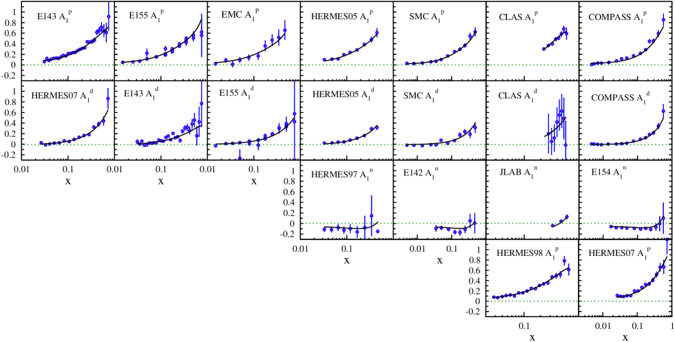
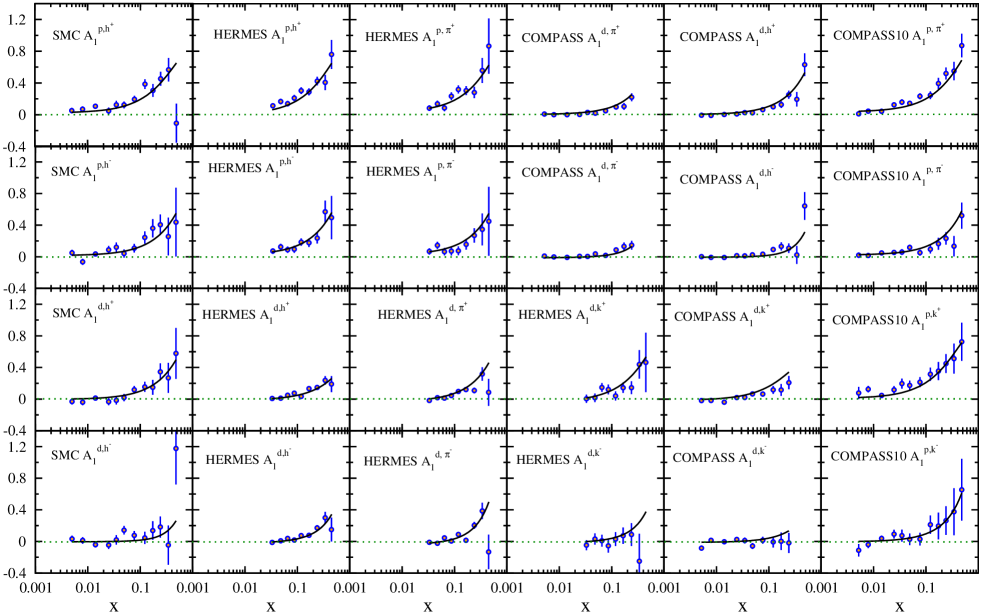
The values of obtained parameters attached to the input PPDFs are summarized in Table 2. We find ${\chi}^{2}/{\rm{d.o.f.}}=1171.571/1132=1.03$ which yields an acceptable fit to the experimental data, the individual $\chi^{2}$ for each set of data is presented in Table. 1. The quality of the QCD fit to DIS and SIDIS asymmetry data is demonstrated in Fig. 3 and Fig. 4. Since we use many number of CLAS DIS data for proton and deuteron CLA1pd and they do not situate in the Figure, we just show 8 of them for presentation. As can be seen the data are generally well described by the curves.

V.2 Extracted polarized parton distributions

In Fig. 5 we present the polarized parton distributions and their comparison to parameterizations from DSSV09 deFlorian:2009vb and LSS10 lss at input scale $Q_{0}^{2}=1$ GeV².

Examining the $x(\delta u+\delta\bar{u})$ and $x(\delta d+\delta\bar{d})$ distributions we see that all of the fits are in agreement. For the $x\delta\bar{u}$ and $x\delta\bar{d}$ distributions, the curves, specially our model and DSSV09, are very close; $\delta\bar{d}$ is negative for any $x$ in the measured $x$ region while $\delta\bar{u}$ passes zero around $x=0.1-0.2$ and becomes negative for large $x$ for all presented models.

Figure 3: Comparison of our NLO QCD results for the DIS asymmetries of proton, neutron and deuteron with the data at measured $x$ and $Q^{2}$.

Figure 4: Comparison of our NLO QCD results for the SIDIS asymmetries with the data at measured $x$ and $Q^{2}$.

Figure 5: The result of our analysis for quark helicity distributions at $Q_{0}^{2}=1$ GeV² in comparison with DSSV09 deFlorian:2009vb and LSS10 lss .

Figure 6: The quark helicity distributions for the difference $x(\delta\bar{u}-\delta\bar{d})$ at $Q^{2}=2.5~{},3$ GeV² comparing to DSSV09 deFlorian:2009vb , LSS10 lss and GRSV01 Gluck:2000dy and experimental data hermespdf ; compass10 .

Figure 7: The quark helicity distributions for $x\delta s$, $x\delta\bar{u}$ and $x\delta\bar{d}$ at $Q_{0}^{2}=2$ GeV² comparing to $x\delta q$ obtained from the previous standard scenario PRD11 .

Figure 8: The comparison of PPDFs results extracted from all datasets shown in Table 1, and the PPDFs results extracted by excluding COMPASS SIDIS datasets at $Q_{0}^{2}=1$ GeV². The corresponding error bands of them are also shown.

Figure 9: The comparison of PPDFs results extracted from sign changing and positive gluon scenarios at $Q_{0}^{2}=1$ GeV². The corresponding error bands of them are also shown.

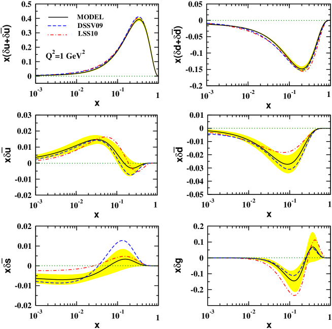
For the strange sea-quark density $x\delta s$, the main difference between the presented model, LSS10 and DSSV09 sets is that for $x<0.03$ LSS10 is less negative than others, also both of current model and LSS10 are less positive than DSSV09 for $x>0.03$. The other differences for the distributions comes from the fact that both DSSV09 and LSS10 analysis uses different number of data (we use the most and the newest ones) and DSSV09 uses pp collision data from RHIC which can impose individual constraints and effects on individual parton distributions in the nucleon deFlorian:2009vb . As we mentioned, in the current analysis we focuss on the study of SIDIS data effect on determination of PPDFs, specially gluon and sea quarks separation which was not considered in our last DIS analysis. The impact of RHIC pp collision data will be considered in our near future analysis.

V.3 The impact of SIDIS data in determining the polarized sea-quark distributions

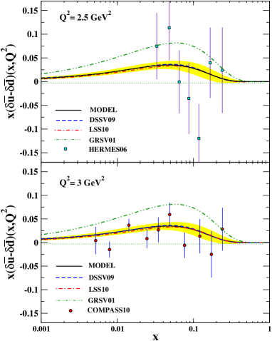
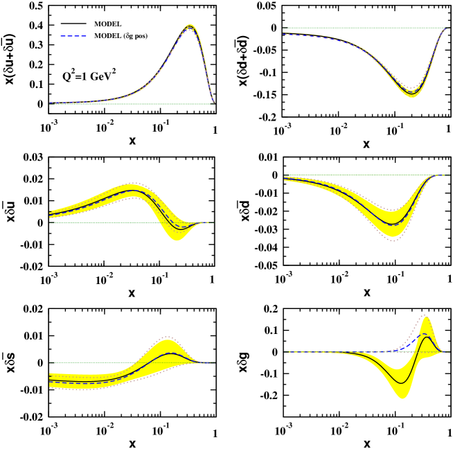
Generally speaking, polarized inclusive DIS data cannot distinguish $\bar{u}$, $\bar{d}$ and $\bar{s}$ but $\delta u=\delta d=\delta s=\delta\bar{s}=\delta\bar{q}$ is well determined and all the standard scenario NLO QCD analysis yield a negative value of it for any $x$ in the measured region Blumlein:2010rn . Employing SIDIS data a flavor decomposition of the polarized sea quarks is obtained and the light antiquark polarized densities $\delta\bar{u}$, $\delta\bar{d}$ and $\delta s=\bar{s}$ are determined separately, Fig. 6 shows the difference between $\delta\bar{u}$, $\delta\bar{d}$ in the current analysis comparing to other models and experimental data.

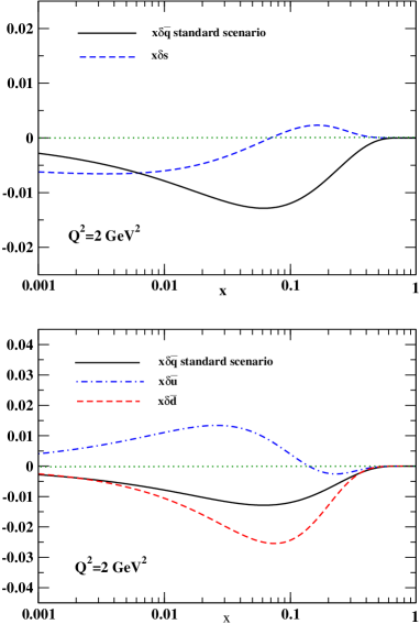
Also in the present parametrization we use a term $(1+c_{s}x^{0.5}+d_{s}x)$ in the input strange sea-quark distribution to let a sign changing for $\delta s=\delta\bar{s}$, which was not considered in the standard scenario PRD11 . The comparison of polarized light sea-quark distributions ($x\delta s,~{}x\delta\bar{u},~{}x\delta\bar{d}$) in the standard scenario and current model are presented in Fig. 7. It shows that the behavior of the polarized strange quark density remains puzzling Leader:2011tm .

Note that by having SIDIS data $\delta s$ and $\delta\bar{s}$ can be separately determined as was done by the COMPASS collaboration recently compass10 . However, it was demonstrated that there is no considerable difference between $\delta s$ and $\delta\bar{s}$ in the $x$-range covered by their data. Also, the errors of the presented values of the difference $\delta s(x)-\delta\bar{s}(x)$ are quite large to allow us to conclude the assumption $\delta s(x)=\delta\bar{s}(x)$ like LSS10 and DSSV09. So, the above assumption and also the form of the fragmentation functions used to extract PPDFs by different groups may be possible causes of the contradiction between sea quarks densities obtained from the analyses of inclusive DIS data and combined inclusive and semi- inclusive DIS datasets Leader:2011tm .

V.4 The effect of COMPASS SIDIS data on polarized sea-quark distributions

As shown in Table 1 The measurement of SIDIS asymmetries for unidentified charged hadrons was performed by SMC collaboration and then the SIDIS asymmetries data for charged pion production from proton target and for charged kaon and pion production from a deuteron target was reported by HERMES. These asymmetries were used in the most DIS and SIDIS QCD analysis but the SIDIS asymmetry data from COMPASS are partially employed, specially the new semi inclusive asymmetries COMPASS data for scattering of muons from a polarized proton target for identified charged pions and kaons production; $A_{1}^{p,\pi^{\pm}}$ and $A_{1}^{p,k^{\pm}}$ compass10 , which was not available for the analysis before 2010.

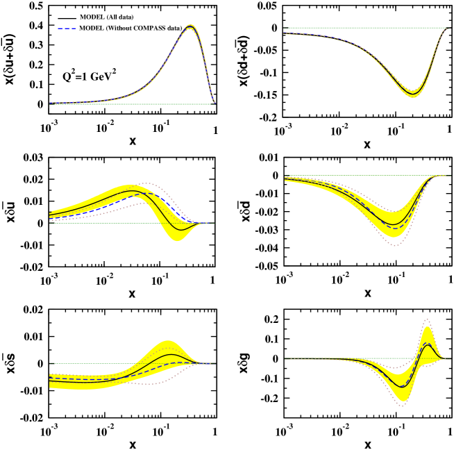
In order to study the effect of COMPASS SIDIS data on polarized parton distributions, we show the comparison of our PPDFs results extracted from all datasets shown in Table 1, and the PPDFs results extracted by excluding COMPASS SIDIS datasets in Fig. 8. As can be seen COMPASS data has effect on $\delta\bar{u}$, $\delta\bar{d}$ and $\delta s=\delta\bar{s}$ distributions since $\pi^{\pm}$ and $k^{\pm}$ are directly related to them. The changes of sea quark distributions are considerable in $0.07\leq x\leq 0.4$ region that is well covered by the new COMPASS data. The distributions of $\delta u+\delta\bar{u}$, $\delta d+\delta\bar{d}$ and $\delta g$ are not changed considerably.

V.5 Gluon polarization

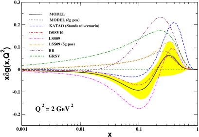
In order to study the effect of SIDIS data on polarized gluon distribution, we perform another analysis with positive polarized gluon distribution. We understand that utilizing polarized DIS and SIDIS data in the QCD analysis can not enforce the positive or sign changing polarized gluon distributions and the data can not distinguish between these two scenarios, although the recent analyses which employ both DIS and SIDIS data (and not pp collision data) could extract sign changing $x\delta g$ lss ; Sissakian:2009ag . In Table. 3 we present the values of obtained parameters in positive gluon scenario. We find ${\chi}^{2}/{\rm{d.o.f.}}=1.02$ which is almost equal to the one obtained from sign changing gluon scenario ${\chi}^{2}/{\rm{d.o.f.}}=1.03$. Fig. 9 shows the comparison of PPDFs extracted from positive and sign changing gluon scenarios. As can be seen all the distributions are almost not changed except $x\delta g$.

flavor	$\eta$	$a$	$b$	$c$	$d$
$u+\bar{u}$	0.770	0.411$\pm$ 0.0955	2.760$\pm$ 0.1356	$0.0^{*}$	78.145$\pm$39.9149
$d+\bar{d}$	-0.498	0.125$\pm$ 0.0080	4.221$\pm$ 0.0359	$0.0^{*}$	67.151$\pm$4.0270
$\bar{u}$	0.051$\pm$ 0.0004	0.411$\pm$ 0.0955	10.0∗	11.231$\pm$ 0.4776	-32.425$\pm$ 0.6351
$\bar{d}$	-0.081$\pm$ 0.0003	0.125$\pm$ 0.0080	10.0∗	85.423$\pm$2.4403	915.221$\pm$ 26.7240
$\bar{s}$	-0.079$\pm$ 0.0387	0.125$\pm$ 0.0080	10.0∗	$0.0^{*}$	-15.843$\pm$3.2887
$g$	0.081$\pm$0.0008	3.958$\pm$ 0.0326	10.0∗	$0.0^{*}$	25.820$\pm$0.8029

Table 3: Final parameter values and their statistical errors at the input scale $Q_{0}^{2}=1$ GeV² for positive gluon scenario, those parameters marked with (*) are fixed.

Fig. 10 shows the gluon distribution comparison between our previous standard scenario and the present sea flavor decomposition analysis. As presented, SU(2) and SU(3) symmetry breaking has direct effect on $x\delta g(x,Q^{2})$ and makes it less. The gluon results of other models of both standard and light sea-quark decomposition scenario are also presented in Fig. 10 and they confirm this effect too deFlorian:2009vb ; lss ; PRD11 ; Gluck:2000dy ; Blumlein:2010rn .

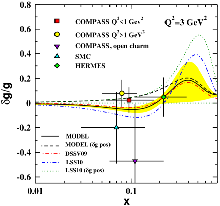
We also calculated the ratio $\delta g/g$, using our extracted PPDFs for polarized gluon distributions and MRST02 Martin:2002aw NLO QCD analysis for unpolarized gluon distributions. In Fig. 11 we present a comparison for $\delta g/g$ from LSS10, DSSV09 and our models (sing changing and positive gluon scenarios) at $Q^{2}=3$ GeV² with measured value from experimental data Airapetian:1999ib ; Adeva:2004dh ; Stolarski:2008jc ; Ageev:2005pq ; Alekseev:2008cz . Although we do not use the mentioned data in the current analysis, our results can predict the data very well.

Figure 10: The gluon helicity distributions at $Q^{2}=2$ GeV² comparing to symmetry breaking deFlorian:2009vb ; lss and standard scenario PRD11 ; Gluck:2000dy ; Blumlein:2010rn analysis.

V.6 Behavior of $\Delta\chi^{2}$

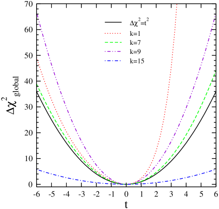
For more deliberation, in the preliminary QCD fit process we let all input parameters to vary. While investigating the behavior of $\Delta\chi^{2}$ we observe $\chi^{2}$ increase consumedly in some points and a big amount of redundance in parameters happens, this redundancy results into disorder of quadratic behavior of $\Delta\chi^{2}$. In order to have the Hessian method work as shown in Sec. IV.2, we fix some parameters at their best obtained value so that Hessian matrix depends on the number of parameters which are independent sufficiently for the quadratic behavior of $\Delta\chi^{2}$, the detailed fixing and constraints in parameter space was discussed in Subsec. III.2 and Sec. IV.

To test of quadratic approximation in Eq. 39, Fig. 12 presents $\Delta\chi^{2}$ along some random samples of eigenvector directions and eigenvalues, $k=1,7,9,15$. The curves for middle values of $\lambda_{k=7,9}$ are very close to the ideal quadratic curve $\Delta\chi^{2}=t^{2}$ and for other eigenvalues $\lambda_{k=1,15}$ we see some departure of ideal quadratic curve which shows the quadratic approximation is almost adequate, though imperfect. The behavior of the some odd curves, which are also available in other QCD analysis Martin:2009iq , usually correspond to the parameters controlling some unknown $x$-dependance parts of sea quarks and gluon densities.

V.7 The spin sum rule

In the framework of QCD the spin $\frac{1}{2}$ of the proton can be defined in terms of the first moment of the total quark and gluon polarized densities and their orbital angular momentum

$$\frac{1}{2}=\frac{1}{2}\Delta\Sigma^{p}+\Delta g^{p}+L_{z}^{p}\;,$$ (48)

where $L_{z}^{p}$ contains the total orbital angular momentum of all partons. The contribution of $\frac{1}{2}\Delta\Sigma+\Delta g$ in the scale of $Q^{2}=4$ GeV² is around $0.010$ in the present analysis. The reported values from DSSV09 deFlorian:2009vb and LSS10 lss are $0.026$ and $-0.212$ respectively. For the positive gluon scenario LSS obtained $0.419$ while our esult is $0.367$. In Table 4 we compare the values of polarized PDFs first moment in NLO approximation with other recent analyses. Since the values of $\frac{1}{2}\Delta\Sigma$ are almost comparable, we observe and conclude that the difference between the reported values of $\frac{1}{2}\Delta\Sigma+\Delta g$ must be caused by different gluon distributions. Indeed, proliferation in PPDFs data for sea quarks from SIDIS experiments eventuates to more accurate results for gluon distribution rather than analysis on DIS data merely, so one cannot yet come to a definite conclusion about the contribution of the orbital angular momentum to the total spin of the proton.

Fit	$\Delta\bar{s}$	$\Delta G$	$\Delta\Sigma$
DSSV09	-0.056	-0.096	0.245
LSS10	-0.063	0.316	0.207
LSS10 ($\delta g$ pos)	-0.055	0.339	0.254
MODEL	-0.042	-0.138	0.256
MODEL ($\delta g$ pos)	-0.046	0.245	0.244

Table 4: First moments of polarized PDFs at $Q^{2}=4$ GeV². The corresponding DSSV09 and LSS10 values are also presented.

The estimation of the valence spin distribution can be written as an accurate relation obtained from inclusive interactions in the experiments. Indeed one obtains the following at LO Alekseev:2007vi

$$\delta u_{v}+\delta d_{v}\sim\frac{36}{5}\frac{g_{1}^{d}}{(1-1.5\omega_{D})}\ ,$$ (49)

which is approximately true at NLO.

	$x$-range	$Q^{2}$	$\Delta u_{v}+\Delta d_{v}$			$\Delta\bar{u}+\Delta\bar{d}$
		(GeV${}^{2})\hskip 5.69054pt\!\!$	Exp.Value	DNS	MODEL	Exp.Value	DNS	MODEL
SMC98	$0.003-0.7$	10	$0.26\pm 0.21\pm 0.11$	0.386	0.454	$0.02\pm 0.08\pm 0.06$	$-0.009$	-0.043
HERMES05	$0.023-0.6$	2.5	$0.43\pm 0.07\pm 0.06$	0.363	0.445	$-0.06\pm 0.04\pm 0.03$	$-0.005$	-0.040
	$0.006-0.7$		$0.40\pm 0.07\pm 0.06$	0.385	0.459	–	$-0.007$	-0.043
COMPASS07	$0-1$	10	$0.41\pm 0.07\pm 0.06$	–	–	$0.0\pm 0.04\pm 0.03$	–	–

Table 5: Evaluations of the first moments $\Delta u_{v}+\Delta d_{v}$ and $\Delta\bar{u}+\Delta\bar{d}$ from SMC SMC98 , HERMES hermespdf and COMPASS Alekseev:2007vi data and also from the DNS analysis deFlorian:2005mw and present model truncated to the range of each relevant experiment. The SMC results were obtained with the assumption of a SU(3) symmetric sea: $\Delta\bar{u}=\Delta\bar{d}=\Delta\bar{s}$.

Theoretically, the first moment of the polarized valence distributions, truncated to the measured range of $x$,

$$\Gamma_{v}(x_{\rm min}<x<x_{\rm max})=\int_{x_{\rm min}}^{x_{\rm max}}\left[\delta u_{v}(x)+\delta d_{v}(x)\right]{\rm d}x\ ,$$ (50)

is obtained and shown for current model and DNS deFlorian:2005mw in Table. 5. We obtain for the full measured range of $x$ in SMC SMC98 , HERMES hermespdf and COMPASS Alekseev:2007vi experiments

$$\Gamma_{v}(0.003<x<0.7) = 0.454\ ,$$ (51)

$$\Gamma_{v}(0.023<x<0.6) = 0.445\ ,$$ (52)

$$\Gamma_{v}(0.006<x<0.7) = 0.459\ ,$$ (53)

at $Q^{2}=10,~{}2.5$ and $10$ GeV² respectively. Our value of $\Gamma_{v}$ confirms the experimental results and the values come from DNS analysis.

An estimation of the sea quark first moment contribution to the nucleon spin can be generated by combining the values of $\Gamma_{v}$, $\Gamma_{1}^{N}$ and $a_{8}$ Alekseev:2007vi

$$\Delta{\overline{u}}+\Delta{\overline{d}}=3\Gamma_{1}^{N}-\frac{1}{2}\Gamma_{v}+\frac{1}{12}a_{8}\ ,$$ (54)

where $\Gamma_{1}^{N}$ is defined as the first moment of polarized structure function $g_{1}$ for the average nucleon $N$ in an isoscalar target: $g_{1}^{N}=(g_{1}^{p}+g_{1}^{n})/2$

$$\Gamma_{1}^{N}(Q^{2}\!=\!10~{}{\rm GeV}^{2})=\int_{0}^{1}g_{1}^{N}(x,Q^{2})\ ,$$ (55)

and ($a_{8}=3F-D$) evaluated from semi-leptonic hyperon decays. The result is reported to be zero for COMPASS experiment as shown in Table 5. The zero value of $\Delta{\overline{u}}+\Delta{\overline{d}}$ suggests that $\Delta{\overline{u}}$ and $\Delta{\overline{d}}$, if they are not zero, must be in opposite sign. Previous estimation by SMC and HERMES are comparable with this supposition and are also given in Table 5. The DNS parametrization, like the present model, finds a positive value for $\Delta{\overline{u}}$ and a negative value for $\Delta{\overline{d}}$, almost equal in absolute value. Opposite signs of $\Delta{\overline{u}}$ and $\Delta{\overline{d}}$ are anticipated in several models, e.g. in Ref. deFlorian:2009vb ; lss ; Gluck:2000dy , see also peng and references inside.

Figure 11: The calculated ratio $\delta g/g$ for DSSV, LSS deFlorian:2009vb ; lss and our model in comparison with experimental data from COMPASS, HERMES and SMC Airapetian:1999ib ; Adeva:2004dh ; Stolarski:2008jc ; Ageev:2005pq ; Alekseev:2008cz at $Q^{2}=3$ GeV².

Figure 12: $\Delta\chi^{2}_{global}$ as a function of $t$ for some random sample eigenvectors.

VI Summary

We have presented a NLO QCD analysis of the polarized DIS and SIDIS data on nucleon. During the analysis we consider SU(2) and SU(3) symmetry breaking scenario i.e. $\delta\bar{u}\neq\delta\bar{d}\neq\delta\bar{s}$, since the available experimental data are not enough to distinguish $\delta s$ from $\delta\bar{s}$, we take them equal $\delta s=\delta\bar{s}$. The role of the semi-inclusive data in determining the polarized sea quarks is discussed and we have found also that the polarized gluon density is still ambiguous, this ambiguity is the main reason that the quark-gluon contribution into the total spin of the proton is still not well determined. We also calculate the error of PPDFs by standard Hessian method and investigate the quadratic behavior of $\Delta\chi^{2}$. Having extracted the polarized PDFs, we compute the first moments of them and discuss about sum rules.In general, we find good agreement with the experimental data, and our results are in accord with other determinations specially DSSV09 and LSS10 which are the most precise ones. In conclusion, this demonstrates progress of the field toward a detailed description of the spin structure of the nucleon Soffer:2011wb ; Shevchenko:2011nq ; Leader:2010gz ; deFlorian:2010aa ; Sissakian:2009ag ; Boer:2011fh ; deFlorian:2012wk . The results of our new analysis applying pp collision data and studying the impact of fragmentation functions on PPDFs will be presented in a separate publication very soon.

VII Acknowledgments

We thank F. Olness for useful discussions and reading the manuscript. F.A appreciates M. Stratmann from DSSV for kind orientation and E. Kabuss from COMPASS collaboration for communications. A.N.K thanks SITP (Stanford Institute for Theoretical Physics) for partial support and the Physics Department of SMU (Southern Methodist University) for their hospitality during the completion of this work. He is also grateful to CERN TH-PH division for the hospitality where a portion of this work was performed. This project was financially supported by Semnan University, Semnan University Science and Technology Park and the School of Particles and Accelerators, Institute for Research in Fundamental Sciences (IPM).

Appendix A Fortran code

A FORTRAN package containing our polarized parton distributions $x\delta u_{v}(x,Q^{2})$, $x\delta d_{v}(x,Q^{2})$, $x\delta g(x,Q^{2})$, $x\delta\bar{u}(x,Q^{2})$, $x\delta\bar{d}(x,Q^{2})$ and $x\delta s(x,Q^{2})$ at NLO in the $\overline{{\rm MS}}$–scheme can be found in http://particles.ipm.ir/links/QCD.htm code or obtained via e-mail from the authors. These functions are interpolated using cubic splines in $Q^{2}$ and a linear interpolation in $\log\,(Q^{2})$. The package includes an example program to illustrate the use of the routines.

Appendix B N-moment of all polarized SIDIS Wilson coefficients

The transformation of Eq. 33 gives the SIDIS Wilson coefficients in $N-z$ space

$$C_{qq}(N,z) = C_{f}\left\{-8\delta(1-z)+\tilde{P}_{qq}(z)\ln\frac{Q^{2}}{M^{2}}+L_{1}(z)\right.$$ (56)

$$+L_{2}(z)+(1-z)+\delta(1-z)\left[\right.\left(\right.\frac{1}{N}+\frac{1}{1+N}$$

$$-2\gamma-2\Psi(N)-\frac{2}{N}-\frac{2}{N+1}+\frac{3}{2}\left.\right)\ln\frac{Q^{2}}{M^{2}}$$

$$+\frac{1}{6}\left(\right.\frac{3}{N^{2}}+\frac{3}{(1+N)^{2}}+6\gamma(\gamma+\frac{1}{N}+\frac{1}{1+N})$$

$$+\pi^{2}+3\Psi(N)\times(4\gamma+\Psi(N))+3\Psi^{2}(N+2)$$

$$-6\frac{d\Psi(N)}{dN}\left.\right)-\left(\right.-\frac{1}{N^{2}}+\frac{1}{(1+N)^{2}}$$

$$-2\zeta(2,N+1)\left.\right)+\frac{1}{N+N^{2}}\left.\right]$$

$$-2(\gamma+\Psi(N))\frac{1}{(1-z)_{+}}+(1+z)(\gamma+\Psi(N))$$

$$-(\frac{1}{N}+\frac{1}{1+N})\frac{1}{(1-z)_{+}}$$

$$\left.+\frac{2(1+N+NZ)}{N+N^{2}}-\frac{2(1-z)}{N+N^{2}}\right\}~{},$$

$$C_{gq}(N,z) = C_{f}\left\{\frac{1+(1-z)^{2}}{z}\left[\ln\left(\frac{Q^{2}}{M^{2}}z(1-z)\right)-\gamma\right]\right.$$ (57)

$$-\Psi(N)+z+2\frac{1+2N-Nz}{N+N^{2}}-\frac{1+2N}{Nz+N^{2}z}$$

$$\left.-\frac{2z}{N+N^{2}}\right\}~{},$$

$$C_{qg}(N,z) = \frac{1}{2}\left\{\delta(1-z)\right.$$

$$\times\left[-\frac{2-2N-(2+N+N^{2})(\gamma+\Psi(N))}{N(1+N)(2+N)}\right.$$

$$+\left.\left.\frac{2}{2+3N+N^{2}}\right]\right.$$

$$+\frac{2+N+N^{2}}{2N+3N^{2}+N^{3}}\left[\frac{1}{(1-z)_{+}}\right.\left.\left.+\frac{1}{z}-2\right]\right\}~{},$$

$$\delta C_{qq}(N,z) = C^{1}_{qq}-2C_{f}\frac{1}{N+N^{2}}(1-z)~{},$$ (59)

$$\delta C_{qq}(N,z) = C^{1}_{qq}-2C_{f}\frac{1}{N+N^{2}}z~{},$$ (60)

$$\delta C_{qg}(N,z) = \frac{1}{2}\left\{\delta(1-z)\left[-\frac{2+(N-1)(\gamma+\Psi(N))}{N(1+N)}\right.\right.$$ (61)

$$\left.+\frac{2}{N+N^{2}}\right]$$

$$+\frac{N-1}{N(1+N)}\left[\frac{1}{(1-z)_{+}}\right.\left.\left.+\frac{1}{z}-2\right]\right\}~{},$$

where $C_{f}=4/3$, $\gamma\simeq 0.577216$ and

$$\tilde{P}_{qq}(z) = \frac{1+z^{2}}{(1-z)_{+}}+\frac{3}{2}\delta(1-z)~{},$$ (62)

$$L_{1}(z) = (1+z^{2})\left(\frac{\ln(1-z)}{1-z}\right)~{},$$ (63)

$$L_{2}(z) = \frac{1+z^{2}}{1-z}\ln z~{},$$ (64)

$$\int_{0}^{1}dz~{}f(z)(g(z))_{+} \equiv \int_{0}^{1}dz[f(z)-f(1)]g(z).$$ (65)

References

- (1) J. Ashman et al. [European Muon Collaboration], Phys. Lett. B 206 (1988) 364.
- (2) J. Ashman et al. [European Muon Collaboration], Nucl. Phys. B 328 (1989) 1.
- (3) G. Altarelli, arXiv:0907.1751 [hep-ph].
- (4) M. Anselmino, A. Efremov and E. Leader, Phys. Rept. 261 (1995) 1 [Erratum-ibid. 281 (1997) 399] [arXiv:hep-ph/9501369].
- (5) E. W. Hughes and R. Voss, Ann. Rev. Nucl. Part. Sci. 49 (1999) 303.
- (6) B. Lampe and E. Reya, Phys. Rept. 332 (2000) 1 [arXiv:hep-ph/9810270].
- (7) B. W. Filippone and X. D. Ji, Adv. Nucl. Phys. 26 (2001) 1 [arXiv:hep-ph/0101224].
- (8) J. Ashman et al. [European Muon Collaboration], Phys. Lett. B 206 (1988) 364; J. Ashman et al. [European Muon Collaboration], Nucl. Phys. B 328 (1989) 1.
- (9) B. Adeva et al. [Spin Muon Collaboration], Phys. Rev. D 58 (1998) 112001.
- (10) M. G. Alekseev et al. [COMPASS Collaboration], Phys. Lett. B 690, 466 (2010) [arXiv:1001.4654 [hep-ex]], V. Y. Alexakhin et al. [COMPASS Collaboration], Phys. Lett. B 647 (2007) 8 [arXiv:hep-ex/0609038].
- (11) P. L. Anthony et al. [E142 Collaboration], Phys. Rev. D 54 (1996) 6620 [arXiv:hep-ex/9610007].
- (12) K. Abe et al. [E143 collaboration], Phys. Rev. D 58 (1998) 112003 [arXiv:hep-ph/9802357].
- (13) K. Abe et al. [E154 Collaboration], Phys. Rev. Lett. 79 (1997) 26 [arXiv:hep-ex/9705012].
- (14) P. L. Anthony et al. [E155 Collaboration], Phys. Lett. B 493 (2000) 19 [arXiv:hep-ph/0007248].
- (15) P. L. Anthony et al. [E155 Collaboration], Phys. Lett. B 463 (1999) 339 [arXiv:hep-ex/9904002].
- (16) A. Airapetian et al. [HERMES Collaboration], Phys. Rev. D 71 (2005) 012003 [arXiv:hep-ex/0407032].
-
(17)
K. Ackerstaff et al. [HERMES Collaboration], Phys. Lett. B 404 (1997) 383 [arXiv:hep-ex/9703005],
A. Airapetian et al. [HERMES Collaboration], Phys. Lett. B 442 (1998) 484 [arXiv:hep-ex/9807015] - (18) A. Airapetian et al. [HERMES Collaboration], Phys. Rev. D 75 (2007) 012007 [arXiv:hep-ex/0609039].
- (19) X. Zheng et al. (JLab/Hall A Collaboration), Phys. Rev. Lett. 92, 012004 (2004); Phys. Rev. C 70, 065207 (2004).
- (20) K. V. Dharmawardane et al. [CLAS Collaboration], Phys. Lett. B 641 (2006) 11 [arXiv:nucl-ex/0605028].
- (21) R. D. Ball et al. [The NNPDF Collaboration], Nucl. Phys. B 874, 36 (2013) [arXiv:1303.7236 [hep-ph]].
- (22) A. N. Khorramian, S. Atashbar Tehrani, S. Taheri Monfared, F. Arbabifar and F. I. Olness, Phys. Rev. D 83 (2011) 054017 [arXiv:1011.4873 [hep-ph]].
- (23) T. Gehrmann and W. J. Stirling, Phys. Rev. D 53 (1996) 6100, hep-ph/9512406.
- (24) J. Blumlein and H. Bottcher, Nucl. Phys. B 841 (2010) 205 [arXiv:1005.3113 [hep-ph]].
- (25) G. Altarelli, R. D. Ball, S. Forte and G. Ridolfi, Acta Phys. Polon. B 29 (1998) 1145 [arXiv:hep-ph/9803237].
- (26) R. D. Ball, G. Ridolfi, G. Altarelli and S. Forte, arXiv:hep-ph/9707276.
- (27) C. Bourrely, F. Buccella, O. Pisanti, P. Santorelli and J. Soffer, Prog. Theor. Phys. 99 (1998) 1017 [arXiv:hep-ph/9803229].
- (28) L. E. Gordon, M. Goshtasbpour and G. P. Ramsey, Phys. Rev. D 58 (1998) 094017 [arXiv:hep-ph/9803351].
- (29) E. Leader, A. V. Sidorov and D. B. Stamenov, Phys. Lett. B 462 (1999) 189 [arXiv:hep-ph/9905512]; E. Leader, A. V. Sidorov and D. B. Stamenov, Phys. Lett. B 445 (1998) 232 [arXiv:hep-ph/9808248], E. Leader, A. V. Sidorov and D. B. Stamenov, Phys. Rev. D 58 (1998) 114028 [arXiv:hep-ph/9807251]; E. Leader, A. V. Sidorov and D. B. Stamenov, Int. J. Mod. Phys. A 13 (1998) 5573 [arXiv:hep-ph/9708335].
- (30) M. Stratmann, Nucl. Phys. Proc. Suppl. 79 (1999) 538 [arXiv:hep-ph/9907465].
- (31) D. K. Ghosh, S. Gupta and D. Indumathi, Phys. Rev. D 62 (2000) 094012 [arXiv:hep-ph/0001287].
- (32) M. Gluck, E. Reya, M. Stratmann and W. Vogelsang, Phys. Rev. D 63, 094005 (2001) [arXiv:hep-ph/0011215].
- (33) R. S. Bhalerao, Phys. Rev. C 63 (2001) 025208 [arXiv:hep-ph/0003075].
- (34) E. Leader, A. V. Sidorov and D. B. Stamenov, Eur. Phys. J. C 23 (2002) 479 [arXiv:hep-ph/0111267].
- (35) J. Blumlein and H. Bottcher, Nucl. Phys. B 636 (2002) 225 [arXiv:hep-ph/0203155].
- (36) Y. Goto et al. [Asymmetry Analysis collaboration], Phys. Rev. D 62 (2000) 034017 [arXiv:hep-ph/0001046]; M. Hirai, S. Kumano and N. Saito [Asymmetry Analysis Collaboration], Phys. Rev. D 69 (2004) 054021 [arXiv:hep-ph/0312112].
- (37) E. Leader, A. V. Sidorov and D. B. Stamenov, Phys. Rev. D 73 (2006) 034023 [arXiv:hep-ph/0512114].
- (38) C. Bourrely, J. Soffer and F. Buccella, “A statistical approach for polarized parton distributions,” Eur. Phys. J. C 23 (2002) 487 [arXiv:hep-ph/0109160].
(39)
G. Altarelli et al., Nucl. Phys. B496 (1997)
337; Acta Phys. Pol. B29 (1998) 1145;
S. Forte, M. Mangano, and G. Ridolfi, Nucl. Phys. B602 (2001) 585. - (40) G. Altarelli, R. D. Ball, S. Forte and G. Ridolfi, “Determination of the Bjorken sum and strong coupling from polarized structure functions,” Nucl. Phys. B 496 (1997) 337 [arXiv:hep-ph/9701289].
- (41) M. Hirai and S. Kumano [Asymmetry Analysis Collaboration], Nucl. Phys. B 813, 106 (2009) [arXiv:0808.0413 [hep-ph]].
- (42) A. N. Khorramian, A. Mirjalili and S. A. Tehrani, JHEP 0410 (2004) 062 [arXiv:hep-ph/0411390].
- (43) S. Atashbar Tehrani and A. N. Khorramian, JHEP 0707, 048 (2007) [arXiv:0705.2647 [hep-ph]].
- (44) S. Atashbar Tehrani, A. N. Khorramian, S. Taheri Monfared and F. Arbabifar, AIP Conf. Proc. 1374, 391 (2011).
- (45) F. Arbabifar, A. N. Khorramian, S. Taheri Monfared and S. Atashbar Tehrani, Int. J. Mod. Phys. A 26, 625 (2011).
- (46) A. N. Khorramian, S. Atashbar Tehrani, F. Olness, S. Taheri Monfared and F. Arbabifar, Nucl. Phys. Proc. Suppl. 207-208, 65 (2010).
- (47) SMC Collaboration, B. Adeva et al., Phys. Lett. B 420 (1998) 180.
- (48) M.G. Alekseev et al. (COMPASS Collaboration), Phys. Lett. B 660, 458 (2008).
- (49) M.G. Alekseev et al. (COMPASS Collaboration), Phys. Lett. B 680, 217 (2009).
- (50) E. Leader, A. V. Sidorov and D. B. Stamenov, Phys. Rev. D 82 (2010) 114018 [arXiv:1010.0574 [hep-ph]].
- (51) D. de Florian, O. A. Sampayo, and R. Sassot, Phys. Rev. D 57, 5803 (1998); D. de Florian and R. Sassot, Phys. Rev. D 62, 094025 (2000); D. de Florian, G. A. Navarro, and R. Sassot, Phys. Rev. D 71, 094018 (2005).
- (52) D. de Florian and R. Sassot, Phys. Rev. D 62 (2000) 094025 [arXiv:hep-ph/0007068].
- (53) D. de Florian, G. A. Navarro and R. Sassot, Phys. Rev. D 71 (2005) 094018 [arXiv:hep-ph/0504155].
- (54) D. de Florian, R. Sassot, M. Stratmann and W. Vogelsang, Phys. Rev. Lett. 101, 072001 (2008) [arXiv:0804.0422 [hep-ph]].
- (55) D. de Florian, R. Sassot, M. Stratmann and W. Vogelsang, Phys. Rev. D 80 (2009) 034030 [arXiv:0904.3821 [hep-ph]].
- (56) M. Soleymaninia, A. N. Khorramian, S. M. Moosavinejad and F. Arbabifar, Phys. Rev. D 88, 054019 (2013) [arXiv:1306.1612 [hep-ph]].
- (57) M. G. Alekseev et al. [COMPASS Collaboration], Phys. Lett. B 693 (2010) 227 [arXiv:1007.4061 [hep-ex]].
- (58) M. Arneodo et al. (NMC Collaboration), Phys. Lett. B 364, 107 (1995).
- (59) K. Abe et al. (SLAC E143 Collaboration), Phys. Lett. B 452, 194 (1999).
- (60) S. D. Bass, Rev. Mod. Phys. 77, 1257 (2005) [hep-ph/0411005].
- (61) D. Adams et al., SMC Collaboration, Phys. Lett. B 336 (1994) 125.
- (62) K. Abe et al., E154 Collaboration, Phys. Lett. B404 (1997) 377.
- (63) S. Wandzura, F. Wilczek, Phys. Lett. B 72 (1977) 195.
- (64) D. de Florian, M. Stratmann, and W. Vogelsang, Phys. Rev. D 57, 5811 (1998).
- (65) A. N. Sisakian, O. Y. .Shevchenko and V. N. Samoilov, hep-ph/0010298.
- (66) E. Leader, A. V. Sidorov and D. B. Stamenov, arXiv:1212.3204.
- (67) M. Hirai, S. Kumano, T. -H. Nagai and K. Sudoh, Phys. Rev. D 75, 094009 (2007) [hep-ph/0702250].
- (68) S. Albino, B. A. Kniehl and G. Kramer, Nucl. Phys. B 803, 42 (2008) [arXiv:0803.2768 [hep-ph]].
- (69) D. de Florian, R. Sassot, and M. Stratmann, Phys. Rev. D 75, 114010 (2007); Phys. Rev. D 76, 074033 (2007).
- (70) A. D. Martin, R. G. Roberts, W. J. Stirling and R. S. Thorne, Eur. Phys. J. C 28, 455 (2003) [hep-ph/0211080].
- (71) J. Soffer, Phys. Rev. Lett. 74, 1292 (1995) [hep-ph/9409254].
- (72) C. Amsler et al. (Particle Data Group), Phys. Lett. B 667 (2008) 1.
- (73) H. J. Lipkin, Phys. Lett. B 214, 429 (1988); Phys. Lett. B 230, 135 (1989); F. E. Close and R. G. Roberts, Phys. Rev. Lett. 60, 1471 (1988); M. Roos, Phys. Lett. B 246, 179 (1990); Z. Dziembowski and J. Franklin, J. Phys. G 17, 213 (1991). P. G. Ratcliffe, Phys. Lett. B 242, 271 (1990); Phys. Lett. B 365, 383 (1996); arXiv:hep-ph/0012133; S. L. Zhu, G. Sacco, and M. J. Ramsey-Musolf, Phys. Rev. D 66, 034021 (2002); E. Leader and D. B. Stamenov, Phys. Rev. D 67, 037503 (2003).
- (74) M. A. Ahmed and G. G. Ross, Nucl. Phys. B 111, 441 (1976); G. Altarelli and G. Parisi, Nucl. Phys. B 126, 298 (1977).
- (75) R. Mertig and W. L. van Neerven, Z. Phys. C 70, 637 (1996); W. Vogelsang, Phys. Rev. D 54, 2023 (1996); Nucl. Phys. B 475, 47 (1996).
- (76) M. Stratmann and W. Vogelsang, Phys. Rev. D 64, 114007 (2001).
- (77) G. Altarelli, R. K. Ellis, G. Martinelli and S. Y. Pi, Nucl. Phys. B 160, 301 (1979).
- (78) A. Vogt, Comput. Phys. Commun. 170, 65 (2005) [arXiv:hep-ph/0408244].
- (79) F. James, MINUIT, CERN Program Library Long Writeup D506.
- (80) A. D. Martin, W. J. Stirling, R. S. Thorne and G. Watt, Eur. Phys. J. C 63, 189 (2009) [arXiv:0901.0002 [hep-ph]].
- (81) J. Pumplin, D. Stump, R. Brock, D. Casey, J. Huston, J. Kalk, H. L. Lai and W. K. Tung, Phys. Rev. D 65, 014013 (2001) [hep-ph/0101032].
- (82) E. Leader, A. V. Sidorov and D. B. Stamenov, Phys. Rev. D 84, 014002 (2011) [arXiv:1103.5979 [hep-ph]].
- (83) A. Sissakian, O. Shevchenko and O. Ivanov, Eur. Phys. J. C 65, 413 (2010) [arXiv:0908.3296 [hep-ph]].
- (84) A. Airapetian et al. [HERMES Collaboration], Phys. Rev. Lett. 84, 2584 (2000) [hep-ex/9907020].
- (85) B. Adeva et al. [Spin Muon (SMC) Collaboration], Phys. Rev. D 70, 012002 (2004) [hep-ex/0402010].
- (86) M. Stolarski [COMPASS Collaboration], arXiv:0809.1803 [hep-ex].
- (87) E. S. Ageev et al. [COMPASS Collaboration], Phys. Lett. B 633, 25 (2006) [hep-ex/0511028].
- (88) M. Alekseev et al. [COMPASS Collaboration], arXiv:0802.3023 [hep-ex].
- (89) M. Alekseev et al. [COMPASS Collaboration], Phys. Lett. B 660, 458 (2008) [arXiv:0707.4077 [hep-ex]].
- (90) J.C. Peng, Eur. Phys. J. A18 (2003) 395.
- (91) J. Soffer, arXiv:1112.0304 [hep-ph].
- (92) O. Y. Shevchenko, R. R. Akhunzyanov and V. Y. Lavrentyev, Eur. Phys. J. C 71, 1713 (2011) [arXiv:1106.4795 [hep-ph]].
- (93) E. Leader, A. V. Sidorov and D. B. Stamenov, arXiv:1012.5033 [hep-ph].
- (94) D. de Florian and W. Vogelsang, Phys. Rev. D 81, 094020 (2010) [arXiv:1003.4533 [hep-ph]].
- (95) D. Boer et al., arXiv:1108.1713 [nucl-th].
- (96) D. de Florian and Y. R. Habarnau, Eur. Phys. J. C 73, 2356 (2013) [Eur. Phys. J. C 73, 2356 (2013)] [arXiv:1210.7203 [hep-ph]].
- (97) Program summary: http://particles.ipm.ir/links/QCD.htm.