Acoustic scaling of anisotropic flow in shape-engineered events: implications for
extraction of the specific shear viscosity of the quark gluon plasma

Abstract

It is shown that the acoustic scaling patterns of anisotropic flow for different event shapes at a fixed collision centrality (shape-engineered events), provide robust constraints for the event-by-event fluctuations in the initial-state density distribution from ultrarelativistic heavy ion collisions. The empirical scaling parameters also provide a dual-path method for extracting the specific shear viscosity $(\eta/s)_{\mathrm{QGP}}$ of the quark-gluon plasma (QGP) produced in these collisions. A calibration of these scaling parameters via detailed viscous hydrodynamical model calculations, gives $(\eta/s)_{\mathrm{QGP}}$ estimates for the plasma produced in collisions of Au+Au ($\sqrt{s_{NN}}=0.2$ TeV) and Pb+Pb ($\sqrt{s_{NN}}=2.76$ TeV). The estimates are insensitive to the initial-state geometry models considered.

Considerable attention has been given to the study of anisotropic flow measurements in heavy-ion collisions at both the Relativistic Heavy Ion Collider (RHIC) and the Large Hadron Collider (LHC) Teaney (2003); Lacey and Taranenko (2006); Lacey et al. (2007); *Adare:2006nq; *Drescher:2007cd; *Dusling:2007gi; *Xu:2007jv; *Molnar:2008xj; *Lacey:2009xx; *Dusling:2009df; *Chaudhuri:2009hj; *Lacey:2010fe; Romatschke and Romatschke (2007); Luzum and Romatschke (2008); *Luzum:2009sb; Song et al. (2011a); Aamodt et al. (2010); *Luzum:2010ag; Lacey et al. (2011a); Bozek et al. (2010); Hirano et al. (2011); Schenke et al. (2011a); *Schenke:2011tv; Song et al. (2011b); *Shen:2010uy; *Gardim:2012yp; Niemi et al. (2012); Qin et al. (2010). Recently, the attack has focused on studies of initial state fluctuations and their role in the extraction of the specific shear viscosity (i.e. the ratio of shear viscosity to entropy density $\eta/s$) of the quark-gluon plasma (QGP) . These flow measurements are routinely quantified as a function of collision centrality (cent) and particle transverse momentum $p_{\rm{T}}$ by the Fourier coefficients $v_{n}$

$$v_{n}(p_{\rm{T}},{\rm cent})=\langle\cos[n(\phi-\Psi_{\rm n})]\rangle.$$ (1)

Here $\phi$ is the azimuthal angle of an emitted particle and $\Psi_{\rm n}$ is the estimated azimuth of the $n$-th order event plane Ollitrault (1992); Adare et al. (2010); brackets denote averaging over particles and events. The current measurements for charged hadrons Lacey (2011); Adare et al. (2011); *ALICE:2011ab; *ATLAS:2012at; *Sorensen:2011fb; *Sanders:2012iz indicate significant odd and even $v_{n}$ coefficients up to about the sixth harmonic.

The estimates of $(\eta/s)_{\mathrm{QGP}}$ from these $v_{n}$ measurements have indicated a small value (i.e. 1-3 times the lower conjectured bound of ${1}/{4\pi}$ Kovtun et al. (2005)). Substantial theoretical uncertainties have been assigned primarily to incomplete knowledge of the initial-state geometry and its associated event-by-event fluctuations. Indeed, an uncertainty of ${\cal O}(100\%)$ in the value of $(\eta/s)_{\mathrm{QGP}}$ extracted from $v_{2}$ measurements at RHIC ($\mbox{$\sqrt{s_{{}_{\rm NN}}}$}=0.2$ TeV) Luzum and Romatschke (2008); Song et al. (2011a), has been attributed to a $\sim 20$% uncertainty in the theoretical estimates Hirano et al. (2006); Drescher et al. (2006); *Drescher:2007ax; *Qiu:2011iv for the event-averaged initial eccentricity $\varepsilon_{2}$ of the collision zone. Here, it is important to note that a robust method of extraction should not depend on the initial geometrical conditions since $(\eta/s)_{\mathrm{QGP}}$ is only a property of the medium itself.

Recent attempts to reduce the uncertainty for $(\eta/s)_{\mathrm{QGP}}$ have focused on: (i) the development of a more constrained description of the fluctuating initial-state geometry Schenke et al. (2012a), (ii) the combined analysis of $v_{2}$ and $v_{3}$ Lacey et al. (2011b); Adare et al. (2011); *ALICE:2011yba; Shen et al. (2011); *Qiu:2011fi and other higher order harmonics Schenke et al. (2011a, b) and (iii) a search for new constraints via “acoustic scaling” of $v_{n}$ Lacey et al. (2013a, 2011c, b). The latter two approaches [(ii) and (iii)] utilize the prediction that the strength of the dissipative effects which influence the magnitude of $v_{n}({\rm cent})$, grow exponentially as $n^{2}$ and $1/\bar{R}$ Lacey et al. (2013a); Shuryak and Zahed (2013); Lacey et al. (2011c);

$$\frac{v_{n}(\text{cent})}{\varepsilon_{n}(\text{cent})}\propto\exp{\left(-\beta\frac{n^{2}}{{\bar{R}}}\right)},\,\,\,\beta\sim\frac{4}{3}\frac{\eta}{Ts},$$ (2)

where $\varepsilon_{n}$ is the $n$-th order eccentricity moment, $T$ is the temperature and $\bar{R}$ is the initial-state transverse size of the collision zone. Thus, a characteristic linear dependence of $\ln(v_{n}/\varepsilon_{n})$ on $n^{2}$ and $1/\bar{R}$ [cf. Eq. 2], with slopes $\beta^{\prime}\propto(\eta/s)_{\mathrm{QGP}}$ and $\beta^{\prime\prime}\propto(\eta/s)_{\mathrm{QGP}}$ are to be expected.

These scaling patterns have indeed been validated and shown to give important constraints for the extraction of $(\eta/s)_{\mathrm{QGP}}$ from both RHIC ($\mbox{$\sqrt{s_{{}_{\rm NN}}}$}=0.2$ TeV) and LHC ($\mbox{$\sqrt{s_{{}_{\rm NN}}}$}=2.76$ TeV) data Lacey et al. (2013a, 2011c).

Figure 1: (Color online) Calculated values for (a) the $q_{2}$ distribution for 20-25% central events; (b) $\varepsilon_{2}$ vs. $q_{2}$ for 20-25% central events; (c) $\varepsilon_{2,3}$ vs. $q_{2\text{f}}$ for 0-5% central events; (d) $\varepsilon_{2,3}$ vs. $q_{2\text{f}}$ for 20-25% central events. The calculations were made for Pb+Pb collisions at $\mbox{$\sqrt{s_{{}_{\rm NN}}}$}=2.76$ TeV with the MC-Glauber model.

Here, we explore a more explicit constraint for initial-state shape fluctuations, via scaling studies of $v_{n}$ measurements obtained for shape-engineered events, i.e. different event shapes at a fixed centrality.

Such a constraint is derived from the expectation that the event-by-event fluctuations in anisotropic flow, result primarily from fluctuations in the size and shape (eccentricity) of the initial-state density distribution. Thus, various cuts on the full distribution of initial shapes [at a given centrality], should result in changes in the magnitudes of $\langle\varepsilon_{n}\rangle$, $\langle\bar{R_{n}}\rangle$ and $\langle v_{n}\rangle$. Note however, that acceptable models for the initial-state fluctuations should give $\langle\varepsilon_{n}\rangle$ and $\langle\bar{R_{n}}\rangle$ values each of which lead to acoustic scaling of $\langle v_{n}\rangle$ with little, if any, change in the slope parameter $\beta^{\prime}$ ($\beta^{\prime\prime}$) for different event shape selections, i.e., $\beta^{\prime}$ ($\beta^{\prime\prime}$) $\propto(\eta/s)_{\mathrm{QGP}}$ is a property of the medium, not the initial state geometry.

The $q_{n}$ flow vector has been proposed Schukraft et al. (2013) as a tool to select different initial shapes from the distribution of initial-state geometries at a fixed centrality;

$$Q_{n,x}=\sum_{i}^{M}\cos(n\phi_{i});\;Q_{n,y}=\sum_{i}^{M}\sin(n\phi_{i});\;$$ (3)

$$q_{n}=Q_{n}/\sqrt{M},\;$$ (4)

where $M$ is the particle multiplicity and $\phi_{i}$ are the azimuthal angles of the particles in the sub-event used to determine $q_{n}$. We use this technique for model-based evaluations of $\varepsilon_{2}(q_{2},{\rm cent})$ and $\bar{R}(q_{2},{\rm cent})$ to perform validation tests for acoustic scaling of recent $v_{2}(q_{2},{\rm cent})$ measurements, as well as to determine if $\beta^{\prime\prime}$ is independent of event shape. We use the acoustic scaling patterns, indicated in the results of $q_{n}$-averaged viscous hydrodynamical calculations Song et al. (2011c); *cms_ulc_note, to calibrate $\beta^{\prime}\text{ and }\beta^{\prime\prime}$ and make estimates of $(\eta/s)_{\mathrm{QGP}}$ for the plasma produced in Au+Au and Pb+Pb collisions at RHIC and the LHC respectively.

The data employed in this work are taken from measurements by the ALICE and CMS collaborations for Pb+Pb collisions at $\sqrt{s_{NN}}$ = 2.76 TeV Dobrin (2013); Chatrchyan et al. (2013), as well as measurements by the STAR collaboration for Au+Au collisions at $\sqrt{s_{NN}}=200$ GeV Adams et al. (2005); Aamodt et al. (2010). The ALICE measurements Dobrin (2013) exploit a three subevents technique to evaluate $v_{2}(q_{2},{\rm cent})$, where the first subevent $\text{SE}_{1}$ is used to determine $q_{2}$, and the particles in the second subevent $\text{SE}_{2}$ are used to evaluate $v_{2}(q_{2},{\rm cent})$ relative to the $\Psi_{2}$ event plane determined from the particles in the third subevent $\text{SE}_{3}$. To suppress non-flow correlations, the detector subsystems used to select $\text{SE}_{1,2,3}$ were chosen so as to give a sizable pseudo-rapidity gap ($\Delta\eta_{p}$) between the particles in different subevents. For each centrality, $v_{2}(q_{2})$ measurements were made for the full $q_{2}$ distribution [$v_{2}(q_{2(\text{Avg.})})$], as well as for events with the 10% lowest [$v_{2}(q_{2(\text{Lo})})$] and 5% highest [$v_{2}(q_{2(\text{Hi})})$] values of the $q_{2}$ distribution.

The CMS cms and STAR Adams et al. (2005) $v_{n}({\rm cent})$ measurements for $n=2-6$ (CMS) and $n=2$ (STAR) were selected to ensure compatibility with the viscous hydrodynamical calculations discussed below. An explicit selection on $q_{n}$ was not used for these measurements; instead, they were averaged over the respective $q_{n}$ distributions to give $v_{n}(q_{n(\text{Avg.})},{\rm cent})\equiv v_{n}({\rm cent})$. The systematic errors for the ALICE, CMS and STAR measurements are reported in Refs.  Dobrin (2013), Chatrchyan et al. (2013) and Adams et al. (2005) respectively.

Monte Carlo versions were used for (a) the Glauber (MC-Glauber) Miller et al. (2007); *Alver:2006wh and (b) Kharzeev-Levin-Nardi Kharzeev and Nardi (2001); Lappi and Venugopalan (2006); Drescher and Nara (2007) (MC-KLN) models for fluctuating initial conditions. Each was used to compute the number of participants N${}_{\text{part}}(\text{cent})$, $q_{n}({\rm cent})$, $\varepsilon_{n}({\text{cent}})$ [with weight $\omega(\mathbf{r_{\perp}})=\mathbf{r_{\perp}\!}^{n}$] and $\bar{R}_{n}({\text{cent}})$ from the two-dimensional profile of the density of sources in the transverse plane $\rho_{s}(\mathbf{r_{\perp}})$ Lacey et al. (2011b), where ${1}/{\bar{R}_{2}}~{}=~{}\sqrt{\left({1}/{\sigma_{x}^{2}}+{1}/{\sigma_{y}^{2}}\right)}$, with $\sigma_{x}$ and $\sigma_{y}$ the respective root-mean-square widths of the density distributions. Computations for these initial-state geometric quantities were also made for 5% and 10% increments in $q_{n}$, from the lowest ($q_{n(\text{Lo})}$) to the highest ($q_{n(\text{Hi})}$) values of the $q_{n}$ distribution. The computations were performed for both Au+Au ($\sqrt{s_{NN}}=0.2$ TeV) and Pb+Pb ($\sqrt{s_{NN}}=2.76$ TeV) collisions. From variations of the MC-Glauber and MC-KLN model parameters, a systematic uncertainty of 2-3% was obtained for $\bar{R}$ and $\varepsilon$ (respectively) .

Figure 2: (a) (Color online) Centrality dependence of $v_{2}(q_{2\text{(Lo)}})$, $v_{2}(q_{2\text{(Avg.)}})$ and $v_{2}(q_{2\text{(Hi)}})$ Dobrin (2013) for $0<\text{ cent }<70$% for Pb+Pb collisions at $\mbox{$\sqrt{s_{{}_{\rm NN}}}$}=2.76$ TeV. (b) Centrality dependence of the ratios $v_{2}(q_{2\text{(Lo)}})/v_{2}(q_{2\text{(Avg.)}})$ and $v_{2}(q_{2\text{(Hi)}})/v_{2}(q_{2\text{(Avg.)}})$. (c) Centrality dependence of $\varepsilon_{2}(q_{2\text{(Lo)}})$, $\varepsilon_{2}(q_{2\text{(Avg.)}})$ and $\varepsilon_{2}(q_{2\text{(Hi)}})$, evaluated with the MC-Glauber model. (d) $\ln[v_{2}(q_{2})/\varepsilon_{2}(q_{2})]$ vs. $1/\bar{R}_{2}(q_{2})$ for $q_{2(\text{Lo})}$. (e) same as (d) but for $q_{2(\text{Avg.})}$. (f) same as (d) but for $q_{2(\text{Hi})}$.

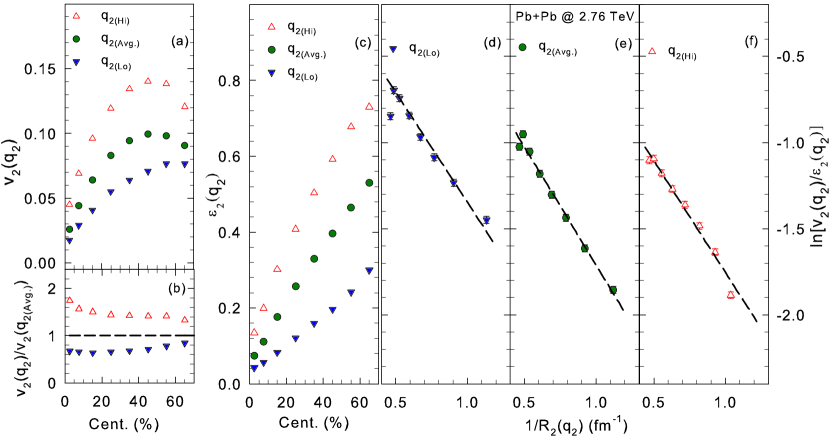
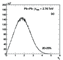
Figure 1(a) shows a representative $q_{2}$ distribution for 20-25% central MC-Glauber events for Pb+Pb collisions. The relatively broad distribution reflects the effects of sizable event-by-event fluctuations convoluted with statistical fluctuations due to finite particle number. Qualitatively similar distributions were obtained for other centralities and for other harmonics. These $q_{n}$ distributions were partitioned into the 5% and 10% increments $q_{n\text{f}}$ [from the lowest to the highest values] and used for further detailed selections on the event shape.

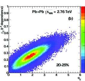
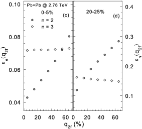
The effectiveness of such selections is illustrated in Fig. 1(b), which shows a strong correlation between $\varepsilon_{2}$ and $q_{2}$ for 20-25% central Pb+Pb events. Similar trends were obtained for other centrality cuts and for other harmonics. Figs. 1(c) and (d) show the dependence of $\varepsilon_{2}$ and $\varepsilon_{3}$ on $q_{2\text{f}}$ for two centrality selections as indicated. For central collisions (0-5%), $\varepsilon_{2}(q_{2\text{f}})$ and $\varepsilon_{3}(q_{2\text{f}})$ both show an increase with $q_{2\text{f}}$, albeit with a much stronger dependence for $\varepsilon_{2}(q_{2\text{f}})$. This increase is expected to lead to a corresponding increase of $v_{2}(q_{2\text{f}})$ and $v_{3}(q_{2\text{f}})$ with $q_{2\text{f}}$.

Fig. 1(d) indicates a similar increase of $\varepsilon_{2}(q_{2\text{f}})$ with $q_{2\text{f}}$ for 20-25% central collisions. However, $\varepsilon_{3}(q_{2\text{f}})$ indicates a decrease with $q_{2\text{f}}$, suggesting that a characteristic inversion of the dependence of $v_{3}(q_{2})$ is to be expected as a signature in future $v_{3}(q_{2})$ measurements for central and mid-central collisions.

Figure 2(a) shows the centrality dependence for one set of the shape-engineered measurements of $v_{2}(q_{2\text{(Lo)}},{\rm cent})$, $v_{2}(q_{2\text{(Avg.)}},{\rm cent})$ and $v_{2}(q_{2\text{(Hi)}},{\rm cent})$ reported in Ref. Dobrin (2013). They show that this event-shape selection leads to lower (higher) values of $v_{2}(q_{2},{\rm cent})$ for $q_{2}$ values lower (higher) than $q_{2\text{(Avg.)}}$. They also show that such selections can lead to a sizable difference (more than a factor of two) between $v_{2}(q_{2\text{(Hi)}},{\rm cent})$ and $v_{2}(q_{2\text{(Lo)}},{\rm cent})$, as illustrated in Fig.  2(b). Strikingly similar differences can be observed in Fig. 2(c) for the MC-Glauber results shown for $\varepsilon_{2}(q_{2\text{(Lo)}},{\rm cent})$, $\varepsilon_{2}(q_{2\text{(Avg.)}},{\rm cent})$ and $\varepsilon_{2}(q_{2\text{(Hi)}},{\rm cent})$. They suggest that differences in the measured magnitudes for $v_{2}(q_{2\text{(Lo)}},{\rm cent})$, $v_{2}(q_{2\text{(Avg.)}},{\rm cent})$ and $v_{2}(q_{2\text{(Hi)}},{\rm cent})$, are driven by the corresponding differences in the calculated magnitudes for $\varepsilon_{2}(q_{2\text{(Lo)}},{\rm cent})$, $\varepsilon_{2}(q_{2\text{(Avg.)}},{\rm cent})$ and $\varepsilon_{2}(q_{2\text{(Hi)}},{\rm cent})$.

The shape-selected measurements in Fig. 2(a) for $v_{2}(q_{2\text{(Lo)}},{\rm cent})$, $v_{2}(q_{2\text{(Avg.)}},{\rm cent})$ and $v_{2}(q_{2\text{(Hi)}},{\rm cent})$ all show an increase from central to mid-central collisions, as would be expected from an increase in $\varepsilon_{2}(q_{2\text{(Lo)}},{\rm cent})$, $\varepsilon_{2}(q_{2\text{(Avg.)}},{\rm cent})$ and $\varepsilon_{2}(q_{2\text{(Hi)}},{\rm cent})$ over the same centrality range [cf. Fig. 2(c)]. For ${\rm cent}\gtrsim 45\%$ however, the decreasing trends for $v_{2}(q_{2\text{(Lo)}},{\rm cent})$, $v_{2}(q_{2\text{(Avg.)}},{\rm cent})$ and $v_{2}(q_{2\text{(Hi)}},{\rm cent})$ contrasts with the increasing trends for $\varepsilon_{2}(q_{2\text{(Lo)}},{\rm cent})$, $\varepsilon_{2}(q_{2\text{(Avg.)}},{\rm cent})$ and $\varepsilon_{2}(q_{2\text{(Hi)}},{\rm cent})$, suggesting that the viscous effects due to the smaller systems produced in peripheral collisions, serve to suppress $v_{2}(q_{2\text{(Lo)}},{\rm cent})$, $v_{2}(q_{2\text{(Avg.)}},{\rm cent})$ and $v_{2}(q_{2\text{(Hi)}},{\rm cent})$. This is confirmed by the symbols and dashed curves in Figs. 2(d) - (f) which validates the expected linear dependence of $\ln[v_{2}(q_{2})/\varepsilon_{2}(q_{2})]$ on $1/\bar{R}_{2}(q_{2})$ (cf. Eq. 2) for the data shown in Fig. 2(a). The dashed curves, which indicate a similar slope value ($\beta^{\prime\prime}\sim 1.3\pm 0.07$) for each of the scaling curves in Figs. 2(d) - (f), provide an invaluable model constraint for the event-by-event fluctuations in the initial-state density distribution, as well as for robust estimates of $\eta/s$.

Figure 3: (Color online) $\ln[v_{2}/\varepsilon_{2}]$ vs. $1/\bar{R}_{2}$ for viscous hydrodynamical calculations Song et al. (2011c) for Au+Au collisions at $\mbox{$\sqrt{s_{{}_{\rm NN}}}$}=0.2$ TeV with (a) MC-Glauber initial-state geometries and (b) MC-KLN initial-state geometries; the dashed-dot and the dotted-dashed curves represent linear fits. Results are shown for several values of $4\pi\eta/s$ as indicated. (c) Calibration curve for $\beta^{\prime\prime}$ vs. $4\pi\eta/s$; the $\beta^{\prime\prime}$ values are obtained from the slopes of the curves shown in (a) and (b). The indicated data points are obtained from a linear fit to $\ln[v_{2}/\varepsilon_{2}]$ vs. $1/\bar{R}_{2}$ for the STAR Au+Au data at $\mbox{$\sqrt{s_{{}_{\rm NN}}}$}=0.2$ TeV Adams et al. (2005); Aamodt et al. (2010)

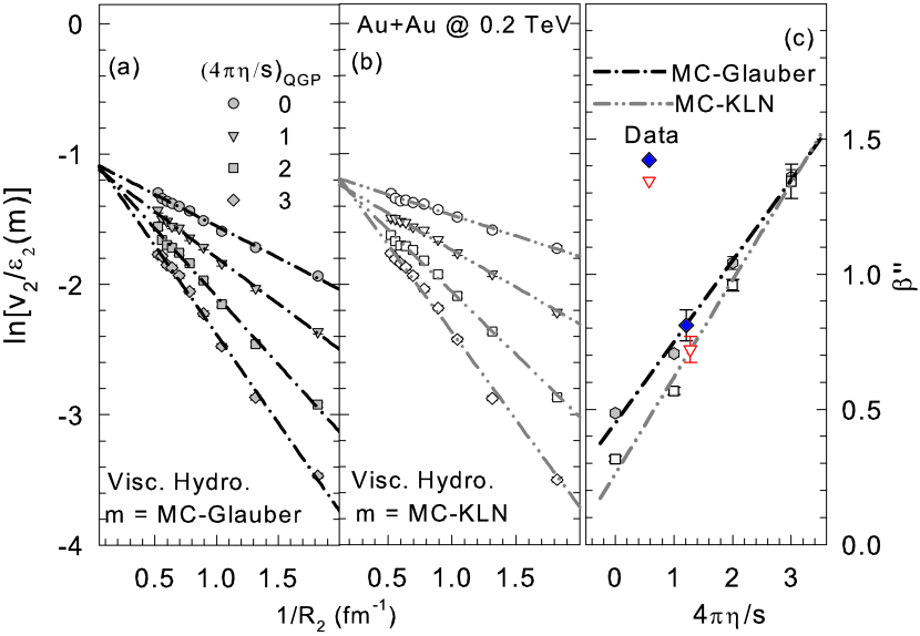
The acoustic scaling patterns summarized in Eq. 2 are also exhibited in the results of $q_{n}$-averaged viscous hydrodynamical calculations Song et al. (2011c); *cms_ulc_note as demonstrated in Figs. 3(a) and (b) and Fig. 4(a). The scaled results, which are shown for several values of $4\pi\eta/s$ in each case, exhibit the expected linear dependence of $\ln(v_{n}/\varepsilon_{n})$ on $1/\bar{R}$ for both MC-Glauber (Figs. 3(a)) and MC-KLN (Figs. 3(b)) initial conditions, as well as the expected linear dependence of $\ln(v_{n}/\varepsilon_{n})$ on $n^{2}$ (Fig. 4(a)). They also give a clear indication that the slopes of these curves are sensitive to the magnitude of $4\pi\eta/s$. Therefore, we use them to calibrate $\beta^{\prime\prime}$ and $\beta^{\prime}$ to obtain estimates for $(4\pi\eta/s)_{\mathrm{QGP}}$ for the plasma produced in RHIC and LHC collisions.

Figure 3(c) shows the calibration curves for $\beta^{\prime\prime}$ vs. $4\pi\eta/s$, obtained from the viscous hydrodynamical calculations shown in Figs. 3(a) and (b). The filled circles and the associated dot-dashed curve, represent the slope parameters ($\beta^{\prime\prime}$) obtained from linear fits to the viscous hydrodynamical results for MC-Glauber initial conditions shown in Fig. 3(a). The open squares and the associated dot-dot-dashed curve, represent the slope parameters obtained from linear fits to the viscous hydrodynamical results for MC-KLN initial conditions shown in Fig. 3(b). The STAR $v_{2}({\rm cent})$ data for Au+Au collisions, also show the expected linear dependence of $\ln(v_{2}/\varepsilon_{2})$ on $1/\bar{R_{2}}$ for $\varepsilon_{2}$ and $\bar{R_{2}}$ values obtained from the MC-Glauber and MC-KLN models respectively. The filled diamond and the open triangle in Fig. 3(c), represent the slopes extracted from the respective scaling plots for MC-Glauber and MC-KLN initial conditions; a comparison to the respective calibration curves in Fig. 3(c), gives the estimate $\langle 4\pi\eta/s\rangle_{\mathrm{QGP}}\sim 1.3\pm 0.2$ for the plasma created in RHIC collisions. Here, it is noteworthy that our extraction procedure leads to an estimate which is basically insensitive to the choice of the MC-Glauber or MC-KLN initial-state geometry.

Figure 4: (Color online) (a) $\ln(v_{n}/\varepsilon_{n})$ vs. $n^{2}$ from viscous hydrodynamical calculations cms for three values of specific shear viscosity as indicated. (b) $\ln(v_{n}/\varepsilon_{n})$ vs. $n^{2}$ for Pb+Pb data. The $p_{T}$-integrated $v_{n}$ results in (a) and (b) are for 0.2% central Pb+Pb collisions at $\sqrt{s_{NN}}=2.76$ TeV cms ; the curves are linear fits. (c) Calibration curve for $\beta^{\prime}$ vs. $4\pi\eta/s$; the $\beta^{\prime}$ values are obtained from the slopes of the curves shown in (a). The indicated data point is obtained from a linear fit to the scaled data shown in (b).

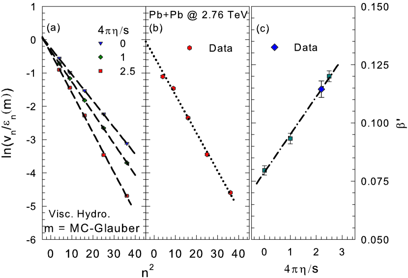
The solid squares and the associated dashed-dot curve in Fig. 4(c), represent the calibration curve for $\beta^{\prime}$ vs. $4\pi\eta/s$, obtained from the linear fits (dashed curves) to the viscous hydrodynamical calculations shown in Fig. 4(a). Fig. 4(b) shows the expected linear dependence of $\ln(v_{n}/\epsilon_{n})$ on $n^{2}$ for CMS Pb+Pb data cms scaled with same $\varepsilon_{n}$ values employed in Fig. 4(a). The slope extracted from Fig. 4(b) is indicated by the solid blue diamond shown in Fig. 4(c); a comparison with the the calibration curve gives the the estimate $\langle 4\pi\eta/s\rangle_{\mathrm{QGP}}\sim 2.2\pm 0.2$ for the plasma created in LHC collisions.

The $\langle 4\pi\eta/s\rangle_{\mathrm{QGP}}$ estimates for the plasma produced in RHIC and LHC collisions are in reasonable agreement with recent $\left<\eta/s\right>$ estimates Lacey et al. (2011c); Schenke et al. (2011b); *Schenke:2011bn; Gale et al. (2012); Qiu et al. (2012). While further calculations will undoubtedly be required to reduce possible model-driven calibration uncertainties, our method benefits from the implicit constraint for the event-by-event fluctuations in the initial-state density distribution, as well as its lack of sensitivity to the initial-state models employed in our analysis.

In summary, we have presented a detailed phenomenological exploration of a new constraint for initial-state fluctuations, via scaling studies of $v_{2}$ measurements obtained for shape-engineered events. We find acoustic scaling patterns for shape-selected events (via $q_{2\text{(Lo)}}$, $q_{2\text{(Avg.)}}$ and $q_{2\text{(Hi)}}$) which provide robust constraints for the event-by-event fluctuations in the initial-state density distribution, as well as methodology with two consistent paths for estimating $(\eta/s)_{\mathrm{QGP}}$ of the QGP produced in Au+Au and Pb+Pb collisions at RHIC and the LHC. A calibration of the method with $q_{2}$-averaged viscous hydrodynamical model calculations, gives estimates for $(4\pi\eta/s)_{\mathrm{QGP}}$ of $1.3\pm 0.2$ and $2.2\pm 0.2$, for the plasma produced in Au+Au ($\sqrt{s_{NN}}=0.2$ TeV) and Pb+Pb ($\sqrt{s_{NN}}=2.76$ TeV) collisions (respectively). These values are insensitive to the initial-state geometry models employed.

Acknowledgments This research is supported by the US DOE under contract DE-FG02-87ER40331.A008.

References

- Teaney (2003) D. Teaney, Phys.Rev. C68, 034913 (2003), arXiv:nucl-th/0301099 [nucl-th] .
- Lacey and Taranenko (2006) R. A. Lacey and A. Taranenko, PoS CFRNC2006, 021 (2006), arXiv:nucl-ex/0610029 [nucl-ex] .
- Lacey et al. (2007) R. A. Lacey, N. Ajitanand, J. Alexander, P. Chung, W. Holzmann, et al., Phys.Rev.Lett. 98, 092301 (2007), arXiv:nucl-ex/0609025 [nucl-ex] .
- Adare et al. (2007) A. Adare et al. (PHENIX Collaboration), Phys.Rev.Lett. 98, 172301 (2007), arXiv:nucl-ex/0611018 [nucl-ex] .
- Drescher et al. (2007) H.-J. Drescher, A. Dumitru, C. Gombeaud, and J.-Y. Ollitrault, Phys.Rev. C76, 024905 (2007), arXiv:0704.3553 [nucl-th] .
- Dusling and Teaney (2008) K. Dusling and D. Teaney, Phys.Rev. C77, 034905 (2008), arXiv:0710.5932 [nucl-th] .
- Xu et al. (2008) Z. Xu, C. Greiner, and H. Stocker, Phys.Rev.Lett. 101, 082302 (2008), arXiv:0711.0961 [nucl-th] .
- Molnar and Huovinen (2008) D. Molnar and P. Huovinen, J.Phys. G35, 104125 (2008), arXiv:0806.1367 [nucl-th] .
- Lacey et al. (2009) R. A. Lacey, A. Taranenko, and R. Wei, (2009), arXiv:0905.4368 [nucl-ex] .
- Dusling et al. (2010) K. Dusling, G. D. Moore, and D. Teaney, Phys.Rev. C81, 034907 (2010), arXiv:0909.0754 [nucl-th] .
- Chaudhuri (2010) A. Chaudhuri, J.Phys. G37, 075011 (2010), arXiv:0910.0979 [nucl-th] .
- Lacey et al. (2010) R. A. Lacey, A. Taranenko, R. Wei, N. Ajitanand, J. Alexander, et al., Phys.Rev. C82, 034910 (2010), arXiv:1005.4979 [nucl-ex] .
- Romatschke and Romatschke (2007) P. Romatschke and U. Romatschke, Phys.Rev.Lett. 99, 172301 (2007), arXiv:0706.1522 [nucl-th] .
- Luzum and Romatschke (2008) M. Luzum and P. Romatschke, Phys.Rev. C78, 034915 (2008), arXiv:0804.4015 [nucl-th] .
- Luzum and Romatschke (2009) M. Luzum and P. Romatschke, Phys.Rev.Lett. 103, 262302 (2009), arXiv:0901.4588 [nucl-th] .
- Song et al. (2011a) H. Song, S. A. Bass, U. Heinz, T. Hirano, and C. Shen, Phys.Rev.Lett. 106, 192301 (2011a), arXiv:1011.2783 [nucl-th] .
- Aamodt et al. (2010) K. Aamodt et al. (ALICE Collaboration), Phys.Rev.Lett. 105, 252302 (2010), arXiv:1011.3914 [nucl-ex] .
- Luzum (2011) M. Luzum, Phys.Rev. C83, 044911 (2011), arXiv:1011.5173 [nucl-th] .
- Lacey et al. (2011a) R. A. Lacey, A. Taranenko, N. Ajitanand, and J. Alexander, Phys.Rev. C83, 031901 (2011a), arXiv:1011.6328 [nucl-ex] .
- Bozek et al. (2010) P. Bozek, M. Chojnacki, W. Florkowski, and B. Tomasik, Phys.Lett. B694, 238 (2010), arXiv:1007.2294 [nucl-th] .
- Hirano et al. (2011) T. Hirano, P. Huovinen, and Y. Nara, Phys.Rev. C83, 021902 (2011), arXiv:1010.6222 [nucl-th] .
- Schenke et al. (2011a) B. Schenke, S. Jeon, and C. Gale, Phys.Rev.Lett. 106, 042301 (2011a), arXiv:1009.3244 [hep-ph] .
- Schenke et al. (2011b) B. Schenke, S. Jeon, and C. Gale, Phys.Lett. B702, 59 (2011b), arXiv:1102.0575 [hep-ph] .
- Song et al. (2011b) H. Song, S. A. Bass, and U. Heinz, Phys.Rev. C83, 054912 (2011b), arXiv:1103.2380 [nucl-th] .
- Shen et al. (2010) C. Shen, U. Heinz, P. Huovinen, and H. Song, Phys.Rev. C82, 054904 (2010), arXiv:1010.1856 [nucl-th] .
- Gardim et al. (2012) F. G. Gardim, F. Grassi, M. Luzum, and J.-Y. Ollitrault, Phys.Rev.Lett. 109, 202302 (2012), arXiv:1203.2882 [nucl-th] .
- Niemi et al. (2012) H. Niemi, G. Denicol, P. Huovinen, E. Molnar, and D. Rischke, Phys.Rev. C86, 014909 (2012), arXiv:1203.2452 [nucl-th] .
- Qin et al. (2010) G.-Y. Qin, H. Petersen, S. A. Bass, and B. Muller, Phys.Rev. C82, 064903 (2010), arXiv:1009.1847 [nucl-th] .
- Ollitrault (1992) J.-Y. Ollitrault, Phys. Rev. D46, 229 (1992).
- Adare et al. (2010) A. Adare et al. (PHENIX), Phys. Rev. Lett. 105, 062301 (2010), arXiv:1003.5586 [nucl-ex] .
- Lacey (2011) R. Lacey (PHENIX Collaboration), J.Phys. G38, 124048 (2011), arXiv:1108.0457 [nucl-ex] .
- Adare et al. (2011) A. Adare et al. (PHENIX Collaboration), Phys.Rev.Lett. 107, 252301 (2011), arXiv:1105.3928 [nucl-ex] .
- Aamodt et al. (2011) K. Aamodt et al. (ALICE Collaboration), Phys.Rev.Lett. 107, 032301 (2011), arXiv:1105.3865 [nucl-ex] .
- Aad et al. (2012) G. Aad et al. (ATLAS Collaboration), Phys.Rev. C86, 014907 (2012), arXiv:1203.3087 [hep-ex] .
- Sorensen (2011) P. Sorensen (STAR Collaboration), J.Phys. G38, 124029 (2011), arXiv:1110.0737 [nucl-ex] .
- Sanders (2012) S. Sanders (CMS Collaboration), PoS QNP2012, 148 (2012).
- Kovtun et al. (2005) P. Kovtun, D. Son, and A. Starinets, Phys.Rev.Lett. 94, 111601 (2005), arXiv:hep-th/0405231 [hep-th] .
- Hirano et al. (2006) T. Hirano, U. W. Heinz, D. Kharzeev, R. Lacey, and Y. Nara, Phys.Lett. B636, 299 (2006), arXiv:nucl-th/0511046 [nucl-th] .
- Drescher et al. (2006) H.-J. Drescher, A. Dumitru, A. Hayashigaki, and Y. Nara, Phys.Rev. C74, 044905 (2006), arXiv:nucl-th/0605012 [nucl-th] .
- Drescher and Nara (2007) H.-J. Drescher and Y. Nara, Phys.Rev. C76, 041903 (2007), arXiv:0707.0249 [nucl-th] .
- Qiu and Heinz (2011) Z. Qiu and U. W. Heinz, Phys.Rev. C84, 024911 (2011), arXiv:1104.0650 [nucl-th] .
- Schenke et al. (2012a) B. Schenke, P. Tribedy, and R. Venugopalan, Phys.Rev.Lett. 108, 252301 (2012a), arXiv:1202.6646 [nucl-th] .
- Lacey et al. (2011b) R. A. Lacey, R. Wei, N. Ajitanand, and A. Taranenko, Phys.Rev. C83, 044902 (2011b), arXiv:1009.5230 [nucl-ex] .
- Snellings (2011) R. Snellings, J.Phys. G38, 124013 (2011), arXiv:1106.6284 [nucl-ex] .
- Shen et al. (2011) C. Shen, S. A. Bass, T. Hirano, P. Huovinen, Z. Qiu, et al., J.Phys. G38, 124045 (2011), arXiv:1106.6350 [nucl-th] .
- Qiu and Heinz (2012) Z. Qiu and U. Heinz, AIP Conf.Proc. 1441, 774 (2012), arXiv:1108.1714 [nucl-th] .
- Lacey et al. (2013a) R. A. Lacey, Y. Gu, X. Gong, D. Reynolds, N. Ajitanand, et al., (2013a), arXiv:1301.0165 [nucl-ex] .
- Lacey et al. (2011c) R. A. Lacey, A. Taranenko, N. Ajitanand, and J. Alexander, (2011c), arXiv:1105.3782 [nucl-ex] .
- Lacey et al. (2013b) R. A. Lacey, A. Taranenko, J. Jia, D. Reynolds, N. Ajitanand, et al., (2013b), arXiv:1305.3341 [nucl-ex] .
- Shuryak and Zahed (2013) E. Shuryak and I. Zahed, (2013), arXiv:1301.4470 [hep-ph] .
- Schukraft et al. (2013) J. Schukraft, A. Timmins, and S. A. Voloshin, Phys.Lett. B719, 394 (2013), arXiv:1208.4563 [nucl-ex] .
- Song et al. (2011c) H. Song, S. A. Bass, U. Heinz, T. Hirano, and C. Shen, Phys.Rev. C83, 054910 (2011c), arXiv:1101.4638 [nucl-th] .
- (53) See Fig. 14 in CMS PAS HIN-12-011.
- Dobrin (2013) A. Dobrin (ALICE Collaboration), Nucl.Phys. A904-905, 455c (2013), arXiv:1211.5348 [nucl-ex] .
- Chatrchyan et al. (2013) S. Chatrchyan et al. (CMS Collaboration), Phys.Rev. C87, 014902 (2013), arXiv:1204.1409 [nucl-ex] .
- Adams et al. (2005) J. Adams et al. (STAR Collaboration), Phys.Rev. C72, 014904 (2005), arXiv:nucl-ex/0409033 [nucl-ex] .
- Miller et al. (2007) M. L. Miller, K. Reygers, S. J. Sanders, and P. Steinberg, Ann. Rev. Nucl. Part. Sci. 57, 205 (2007).
- Alver et al. (2007) B. Alver et al., Phys. Rev. Lett. 98, 242302 (2007).
- Kharzeev and Nardi (2001) D. Kharzeev and M. Nardi, Phys.Lett. B507, 121 (2001), arXiv:nucl-th/0012025 [nucl-th] .
- Lappi and Venugopalan (2006) T. Lappi and R. Venugopalan, Phys. Rev. C74, 054905 (2006).
- Schenke et al. (2012b) B. Schenke, S. Jeon, and C. Gale, Phys.Rev. C85, 024901 (2012b), arXiv:1109.6289 [hep-ph] .
- Gale et al. (2012) C. Gale, S. Jeon, B. Schenke, P. Tribedy, and R. Venugopalan, (2012), arXiv:1210.5144 [hep-ph] .
- Qiu et al. (2012) Z. Qiu, C. Shen, and U. Heinz, Phys.Lett. B707, 151 (2012), arXiv:1110.3033 [nucl-th] .