Planck intermediate results. XVI.
Profile likelihoods for cosmological parameters

Abstract: We explore the 2013 Planck likelihood function with a high-precision multi-dimensional minimizer (Minuit). This allows a refinement of the $\Lambda$CDM best-fit solution with respect to previously-released results, and the construction of frequentist confidence intervals using profile likelihoods. The agreement with the cosmological results from the Bayesian framework is excellent, demonstrating the robustness of the Planck results to the statistical methodology. We investigate the inclusion of neutrino masses, where more significant differences may appear due to the non-Gaussian nature of the posterior mass distribution. By applying the Feldman–Cousins prescription, we again obtain results very similar to those of the Bayesian methodology. However, the profile-likelihood analysis of the CMB combination (Planck+WP+highL) reveals a minimum well within the unphysical negative-mass region. We show that inclusion of the Planck CMB-lensing information regularizes this issue, and provide a robust frequentist upper limit $\sum m_{\nu}\leq 0.26\mathrm{\thinspace e\kern-1.00006ptV}$ (95% confidence) from the CMB+lensing+BAO data combination.

1 Introduction

This paper, one of a set associated with the 2013 release of data from the Planck mission (Planck Collaboration I 2013), describes a frequentist estimation of cosmological parameters using profile likelihoods.

Parameter estimation in cosmology is predominantly performed using Bayesian inference, particularly following the introduction of Markov chain Monte Carlo (MCMC) techniques (Christensen et al. 2001). Many scientists in the field use the sophisticated CosmoMC software (Lewis & Bridle 2002) to study cosmological parameters, and several experiments provide ready-to-use plugins for it. The Planck satellite mission has recently released high-quality data on the cosmic microwave background (CMB) temperature anisotropies. The analysis of the cosmological parameters (Planck Coll. XVI 2013) is based on Bayesian inference using a dedicated version of CosmoMC.

In this methodology, the likelihood leads to the posterior distribution of the parameters once it has been multiplied by some prior distribution that encompasses our knowledge before the measurement is performed. For Planck, wide bounds on uniform distributions have typically been used. However the choice of a particular set of parameters for MCMC sampling, such as the efficient “physical basis” (Kosowsky et al. 2002) used in CosmoMC, may also be viewed as an implicit prior choice.

Frequentist methods do not need priors, other than that some limits on the explored domain are used in practice and can be seen as the bounds of some “uniform priors”. The maximum likelihood estimate (MLE) does not depend on the choice of the set of parameters, since it possesses the property of invariance: if $\hat{\theta}$ represents the MLE of the parameter $\theta$, then the MLE of any function $\tau(\theta)$ is $\hat{\tau}=\tau(\hat{\theta})$. This means that one can compute the MLE with any set of parameters. As we will see in Sect. 2.3, this property is powerful and can be used to obtain asymmetric confidence intervals.

The multi-dimensional solution is only one aspect of parameter estimation and we are also interested in statements on individual parameters. In the MCMC procedure, once the chains have converged this is obtained through marginalization, which is performed by a simple projection of the samples onto one or sometimes two axes. This may however lead to so-called “volume effects”, where the mean of the projected distribution can become incompatible with the multi-dimensional MLE (e.g., Hamann et al. 2007). In the frequentist framework, one instead builds profile likelihoods (Wilks 1938) for individual variables and, by construction, the individual parameter estimates match (up to numerical accuracy) the MLE values.

Such a method has already been used by Yèche et al. (2006) with Wilkinson Microwave Anisotropy Probe (WMAP) data for a nine-parameter fit. The high sensitivity of data from Planck and from the ground-based South Pole Telescope (SPT) and Atacama Cosmology Telescope (ACT) projects requires the simultaneous fit of a larger number of parameters, up to about $40$, with some nuisance ones being poorly constrained. We therefore need to precisely tune a high-quality minimizer, as will be described in this paper.

MCMC sampling is sometimes used to perform a “poor-man’s” determination of the maximum likelihood (e.g., Reid et al. 2010): one bins a given parameter and reports the sample of maximum likelihood in other dimensions. As pointed out in Hamann (2012), in many dimensions it is most likely that the real maximum was never reached in any reasonably-sized chain. The authors suggest changing the temperature of the chain, but this still requires running lengthy evaluations of the likelihood and is less straightforward than directly using a multi-dimensional minimization algorithm.

In this article, we investigate whether the use of priors or marginalization can affect the determination of the cosmological parameters by comparing the published Bayesian results to a frequentist method. For the base $\Lambda$CDM model, it happens that the cosmological parameter posteriors are essentially Gaussian, so it is expected that frequentist and Bayesian methods will lead to similar results. In extensions to the standard $\Lambda$CDM model this is however not true for some parameters (e.g., the sum of neutrino masses), and priors have been shown to play some role in parameter determination (Hamann et al. 2007; Gonzalez-Morales et al. 2011; Hamann 2012). Given the sensitivity of the Planck data, statistical methodologies may matter, and this issue is scrutinized in this work.

In order to build precise profile likelihoods in a high-dimensional space (up to about 40 dimensions), we need a powerful minimizer. We use the mature and widely-used Minuit software (James & Roos 1975). We interfaced it to the modular class Boltzmann solver (Blas et al. 2011) which, from a set of input cosmological parameters, computes the corresponding temperature and polarization power spectra that are tested against the Planck likelihood. This required that we tune the class precision parameters to a level where the numerical noise can be handled by our minimizer, as is described in Sect. 2.1. In Sect. 2.2, we describe our Minuit minimization strategy, and cover in Sect. 2.3 the basics of the frequentist methodology to estimate unknown parameters based on the properties of profile likelihoods. The data sets we use are then discussed in Sect. 3. We give results for the $\Lambda$CDM parameters in Sect. 4.1 and finally investigate, in Sect. 4.2, a case where the posterior distribution is far from Gaussian, namely the neutrino mass case. Additionally, the Appendix gathers some comments on the overall computation time of the method.

2 Method

2.1 The Boltzmann solver: class

To compute the relevant CMB power spectra from a cosmological model, we need a “Boltzmann solver” that numerically evolves the coupled perturbation equations in an expanding universe. While camb is used in the CosmoMC sampler, we prefer to use the class (v1.6) software (Blas et al. 2011). It offers a rigorous way to control the accuracy of output quantities through a comprehensive list of precision parameters (Lesgourgues 2011a). While one can use some high-speed/low-quality settings to perform MCMC sampling because the random nature of the algorithm smooths out discontinuities, this is no longer the case here when searching for an extremum, which requires precise computation of numerical derivatives. Equally, due to computation time, one cannot use precision settings that are too extreme, so a trade-off with Minuit convergence has to be found.

As we will see in Sect. 2.3, 68% confidence intervals are obtained by cutting $\chi^{2}\equiv-2\ln{\cal L}$ values at one. We therefore need the numerical noise to be much less than unity.

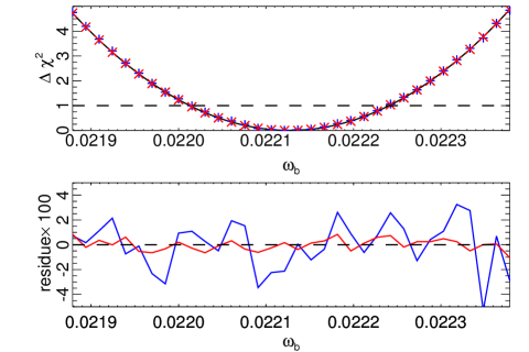
Starting from the Planck likelihood code, described in Sect. 3, we fix all parameters to their published best-fit values (Planck Coll. XVI 2013) and scan a given parameter $\theta$. We compute the $\chi^{2}(\theta)$ curves and subtract a smooth component to estimate the amplitude of the numerical noise. According to the precision settings, trade-off between the amplitude of this noise and the computation time can then be found. An example with two precision settings is shown in Fig. 1 for $\theta=\omega_{\mathrm{b}}=\Omega_{\mathrm{b}}h^{2}$ which is used as our benchmark.

We have determined a set of high-precision settings which achieves sufficient smoothness of the Planck likelihood for the fits to converge, with an increase of only about a factor two in the code computation speed with respect to the default “fast” settings. The values of the settings are reported in Table 1.

Figure 1: Upper panel: the $\omega_{\mathrm{b}}$ parameter is scanned (keeping all other parameters fixed to their best-fit values) and the Planck $\chi^{2}$ values are shown on the vertical axis. Blue points are obtained with the class default settings, and red ones with our high-precision ones. A smooth parabola is fit and shown in black. Lower panel: residuals with respect to the parabola. The r.m.s. of this noise is improved from $0.02$ for the default settings to $0.005$ for the high-precision ones.

class parameter Value

tol_background_integration $$10^{-3}$$

tol_thermo_integration

tol_perturb_integration

reionization_optical_depth_tol

l_logstep

l_linstep

perturb_sampling_stepsize

delta_l_max

Table 1: Values of the non-default precision parameters for class used for the Minuit minimization.

We also found that working with the Thomson scattering optical depth $\tau$ is numerically less stable than using the reionization redshift $z_{\text{re}}$, which defines where the reionization fraction is half of its maximum. We therefore use $z_{\text{re}}$ as a primary parameter. The relation to $\tau$, for a $\tanh$-based ionization profile and a fixed $\Delta z_{\text{re}}=0.5$ width, is given in Lewis (2008).

Since we will compare our results to the previously-published ones, we need to ensure our class configuration reproduces the camb-based results of Planck Collaboration XVI (2013). For this purpose, we use the Planck $\Lambda$CDM best-fit solution and compute its $\chi^{2}$ value and compare with the published results in Table 2. The agreement is good. The slight discrepancy is typical of the differences between class and camb implementations (Lesgourgues 2011b), so we consider our setup to be properly calibrated. From now on, we perform consistent comparisons using only class.

Data set camb class

CMB $$10509.6$$

CMB+BAO

Table 2: Comparison of the $\chi^{2}$ values of the Planck best-fit solution from Planck Collaboration XVI (2013), based on camb, to our class-based implementation, for the CMB and CMB+BAO data sets.

2.2 Minimizing with Minuit

We chose to work with the powerful Minuit package (James & Roos 1975), a well-known minimizer originally developed for high-energy physics and used recently for the Higgs mass determination with a simultaneous fit of 354 parameters (ATLAS Collaboration 2013). While its roots trace back to the 1970s, it has been continually improved and rewritten in C++ as Minuit2, which is the version we use. Minuit is a toolbox including several algorithms that can be deployed depending on the problem under consideration. We refer the reader to the user guide for a detailed description of the procedures we used.

For cosmological parameter estimation with the Planck data, we executed the following strategy

1. Starting from the Planck Collaboration published values and using the high-precision class settings described in Sect. 2.1, we minimize the $\chi^{2}$ function using the MIGRAD algorithm, which is based on Fletcher’s switching algorithm (Fletcher 1970). All parameters are bounded by large (or physical) limits during this exploration.

2. Once a minimum is found, we release all cosmological parameter limits and again perform the MIGRAD minimization. The limits on nuisance parameters are kept in order to avoid exploring unphysical regions.

3. Finally, we use the HESSIAN procedure which refines the local covariance matrix.

MIGRAD belongs to the category of variable metric methods (e.g., Davidon & Laboratory 1959) which build the “expected distance to minimum” (EDM) that represents (twice) the vertical distance to the $\chi^{2}$ minimum if the function is truly quadratic and the gradient exactly known. It can serve as a figure of merit for the convergence and will be used to reject poor fits.

The outcome of this procedure is the minimum $\chi^{2}$ solution together with its Hessian matrix. This solution represents the MLE, but, since the problem is highly non-linear (in particular in $H_{0}$), the Hessian is only a crude approximation to the parameter uncertainties. The complete treatment is through the construction of profile likelihoods.

2.3 Profile likelihoods

The MLE (or “best-fit” or $\chi^{2}_{\mathrm{min}}$) is the global maximum likelihood estimate given the entire set of parameters (cosmological and nuisance). One can choose to isolate one parameter (hereafter called $\theta$) and for fixed values of it look for the maximum of the likelihood function in all other dimensions. One scans $\theta$ within some range and, for each fixed value, runs a minimization with respect to all the other parameters. The minimum $\chi^{2}$ value is reported for this parameter $\theta$, which allows one to build the profile likelihood $\chi^{2}(\theta)$. The procedure ensures the minimum of $\chi^{2}(\theta)$ appears at the same value as the MLE, avoiding the potential volume effects mentioned in the introduction.

A confidence region, which has the correct frequentist coverage properties, can then be extracted from the likelihood ratio statistic, or equivalently the $\Delta\chi^{2}(\theta)=\chi^{2}(\theta)-\chi^{2}_{\mathrm{min}}$ distribution. For a parabolic $\chi^{2}(\theta)$ shape (i.e. Gaussian estimator distribution), a $1-\alpha$ level confidence interval is obtained by the set of values $\Delta\chi^{2}(\theta)\leq\chi^{2}_{1}(\alpha)$, where $\chi^{2}_{1}(\alpha)$ denotes the $1-\alpha$ quantile of the chi-square distribution with one degree of freedom, and is $1,\leavevmode\nobreak\ 2.7$, and $3.84$ for $1-\alpha=68,\leavevmode\nobreak\ 90$ and $95\%$ respectively (e.g., James 2007).

It is less well known that if the profile likelihood is non-parabolic, one can still build an approximate confidence interval using the same recipe, because the full likelihood ratio has the invariance property mentioned in the introduction: one can estimate any monotonic function of $\theta$ and make the same inference not only on the MLE but on any likelihood ratio. For example, one can build the $\Delta\chi^{2}(A_{\rm s})$ distribution from the $\Delta\chi^{2}(\ln(10^{10}A_{\mathrm{s}})))$ profile by simply switching the $\ln(10^{10}A_{\mathrm{s}})\rightarrow A_{\rm s}$ axis. Formally, when the profile likelihood is non-parabolic, one can still imagine a transformation that would make it quadratic in the new variable. One would then apply the parabolic cuts described previously and, by the invariance property, the same inference on the original variable would be obtained. Therefore we can find an (asymmetric) confidence interval by cutting the non-parabolic $\Delta\chi^{2}$ curve at the same $\chi^{2}(\alpha)$ values. This method, sometimes called MINOS (the name of the routine that first implemented it in Minuit), is long known in the statistics field (Wilks 1938). It is exact up to order ${\cal O}(1/N)$ (James 2007), $N$ being the number of samples, and is in practice excellent unless $N$ is very small.

Nevertheless, the profile-likelihood-based confidence intervals must be revisited in the case where the estimate lies near a physical boundary. This will be performed in Sect. 4.2 for the neutrino mass case.

3 Data sets

As our purpose is to compare the frequentist methodology to the Bayesian one, we focus on exactly the same data and parameters as in Planck Collaboration XVI (2013) and refer the reader to Planck Collaboration XV (2013) for their exact definitions. Since the CMB, baryon acoustic oscillation (BAO), and CMB-lensing data were found to be in excellent agreement, we will consider the following likelihood combinations.

The CMB data set consists of the following likelihoods:

• the Planck 2013 data in both low and high $\ell$ ranges;

• the WMAP low-$\ell$ polarization data (referred to as WP in the Planck paper);

• the SPT (Reichardt et al. 2012)+ACT (Das et al. 2013) high-$\ell$ data, referred to as highL.

The combined likelihood, obtained by multiplying the three, includes 31 nuisance parameters, related to the characterization of the unresolved foregrounds, the effective beam, and to the inter-calibration of the Planck and highL power spectra.

The BAO data set consists of a Gaussian likelihood based on the scale measurements from the 6dF (Beutler et al. 2011), SDSS (Padmanabhan et al. 2012), and BOSS (Anderson et al. 2012) experiments, combined as in Planck Collaboration XVI (2013).

For the neutrino mass case, we will also use the Planck lensing likelihood (Planck Collaboration XVII 2013), based on the measurement of the deflection power spectrum.

CMB CMB+BAO

Parameter CosmoMC Minuit CosmoMC Minuit

$$H_{0}$$.

.

.

.

.

.

.

.

.

.

.

.

.

.

.

.

.

.

.

.

.

.

.

.

.

.

.

.

.

.

.

.

.

.

.

.

.

.

Table 3: Best-fit comparison. Values of all parameters at the minimum of the $\chi^{2}$ function as determined by CosmoMC in Planck Collaboration XVI (2013) and by the Minuit implementation described here, for the CMB and CMB+BAO data sets. The first six parameters define the $\Lambda$CDM cosmology. The last line shows the $\chi^{2}$ value at the minimum.

4 Results

4.1 The base $\Lambda$CDM model

We begin by revisiting the global best-fit solution (MLE) using this new minimizer, over all 37 parameters, on the CMB and CMB+BAO data sets. We use the Hubble constant ($H_{0}$) instead of the CMB acoustic scale ($\theta_{\mathrm{MC}}$), which is not available within class, and $z_{\text{re}}$ instead of $\tau$ since it is more stable as discussed in Sect. 2.1. The new minimum is given in Table 3 and compared to the results previously released in Planck Collaboration XVI (2013) , which were obtained with another minimizer. In both cases we find a slightly lower $\chi^{2}$. On the cosmological side we find very similar parameters, except for $z_{\text{re}}$ which is slightly shifted. On the nuisance parameters side, results are also similar, but we are now sensitive to the SZ–CIB cross-correlation parameter $\xi^{\mathrm{tSZ-CIB}}$ while the Planck Collaboration minimum was not shifted from its zero initial value. Additionally the estimated kinetic SZ amplitude $A^{\mathrm{kSZ}}$ is more stable when including the BAO data set.

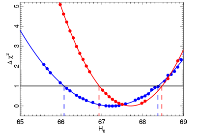
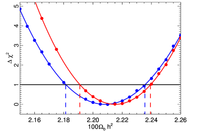
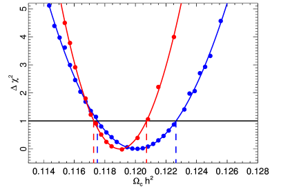
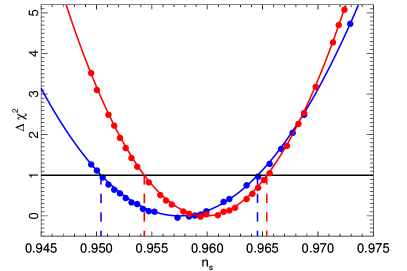
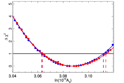
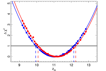
We then build the profile likelihoods by scanning each cosmological parameter and computing the $\chi^{2}$ minimum in the remaining 36 dimensions at each point. Fig. 2 shows the reconstructed profiles. They are found to be mostly parabolic, but we still fit them with a third-order polynomial in order to measure any deviation from a symmetric error, and threshold them at unity in order to obtain the 68% frequentist confidence level interval as explained in Sect. 2.3. Results are reported in Table 4 and compared there to the Planck Collaboration posterior distributions. In most cases the values and errors we obtain are in good agreement with the Bayesian posteriors, demonstrating that the Planck Collaboration results, for the $\Lambda$CDM model, are not biased by a particular choice of parameters (implicit priors) or by the marginalization process (volume effects).

Figure 2: Profile likelihoods ($\Delta\chi^{2}$) reconstructed for each $\Lambda$CDM cosmological parameter, from the CMB (blue) and CMB+BAO (red) data sets. Each point is the result of a 36-parameter minimization. We reject the points that are outliers of the expected distance to minimum (EDM, Sect. 2.2) distribution. Curves are fits to a third-order polynomial. 68% confidence intervals are obtained by thresholding these curves at unity, and their projections onto the parameter axis are shown.

     CMB      CMB+BAO

Parameter      MCMC      Profile-likelihood      MCMC      Profile-likelihood

$$H_{0}$$.                        

.                        

.                        

.                        

.                        

.                        

Table 4: Results of the profile-likelihood analysis (i.e., this work) for the cosmological parameters, using the CMB and CMB+BAO data sets. They are compared to the Planck MCMC posterior results taken from Table 5 of Planck Collaboration XVI (2013).

By comparing the mean values of Table 4 to the best-fit ones (Table 3) we observe that the minima coincide at the percent level, as expected for this frequentist method.

Since we observe some difference in the reionization parameter $z_{\text{re}}$, we also perform the profile-likelihood analysis with the Planck data alone and obtain

$$z_{\text{re}}=13.3^{+2.8}_{-3.3}\qquad(\textsl{Planck-only},\text{profile\leavevmode\nobreak\ likelihood}),$$ (1)

while the Planck Collaboration reports

$$z_{\text{re}}=11.4^{+4.0}_{-2.8}\qquad(\textsl{Planck-only},\text{MCMC\leavevmode\nobreak\ posterior}).$$ (2)

The results, using exactly the same data, are different. We believe that these new results are robust since the profile-likelihood method is particularly well suited for this case. Indeed $z_{\text{re}}$ is fixed in each step so that the minimization does not suffer from the classical $(A_{\rm s},z_{\text{re}}$) degeneracy due to the normalization of the temperature-only power spectrum. In contrast, the MCMC method relies strongly on the priors used on both $A_{\rm s}$ and $z_{\text{re}}$. We find that it is the inclusion of the WMAP polarization data that pulls down this value to $z_{\text{re}}=11.0\pm 1.1$, as reported in Table 4.

4.2 Mass of standard neutrinos

Since the cosmological parameter posterior distributions for the $\Lambda$CDM model are mostly Gaussian (parabolic $\chi^{2}$), the Bayesian and frequentist approaches lead to similar results. However, we may expect greater differences when including neutrino masses in the model, for which the marginalized posterior distribution is peaked towards zero.

CMB measurements are sensitive to the sum of neutrino mass eigenstates $\sum m_{\nu}$ through several effects reviewed in detail in Lesgourgues et al. (2013). For large values $\sum m_{\nu}\gtrsim 1.3\mathrm{\thinspace e\kern-1.00006ptV}$, the neutrinos’ non-relativistic transition happens before decoupling and the integrated Sachs–Wolfe effect reduces the amplitude of the first acoustic peak. For lower mass values, neutrino free-streaming erases small-scale matter fluctuations and accordingly reduces the CMB lensing power. This in turn affects the lensed $C_{\ell}$ spectrum, especially its high-$\ell$ part, and explains the gain when including SPT/ACT data. Furthermore, since according to oscillation experiments at least two neutrinos are non-relativistic today (Beringer et al. 2012), the matter–radiation equality scale factor, which is strongly constrained by the Planck data, reads:

$$\frac{a_{\mathrm{eq}}}{a_{0}}=\frac{\omega_{\mathrm{r}}}{\omega_{\mathrm{m}}-\omega_{\nu}},$$ (3)

where $\omega_{\mathrm{r}}$, $\omega_{\mathrm{m}}$, and $\omega_{\nu}$ are the physical densities of radiation, matter, and massive neutrinos respectively, i.e. $\omega_{\mathrm{r}}=\Omega_{\mathrm{r}}h^{2}$, $\omega_{\mathrm{m}}=\Omega_{\mathrm{m}}h^{2}$, and $\omega_{\nu}=\Omega_{\nu}h^{2}\simeq 10^{-3}\sum m_{\nu}/0.1\mathrm{\thinspace e\kern-1.00006ptV}$. The quantities $\omega_{\nu}$ and $\omega_{\mathrm{m}}$ are clearly degenerate, and so any data set that helps in reducing the CMB geometrical degeneracies by providing a measurement at another scale indirectly benefits $\sum m_{\nu}$. Robust observables, compatible with the Planck $\Lambda$CDM cosmology, are the BAO scale measurement around $z\simeq 0.5$ and/or the CMB-lensing trispectrum that probes matter structures around $z\simeq 2$.

An unexpected result found by Planck Collaboration XVI (2013) is that the 95% confidence upper limit on $\sum m_{\nu}$ obtained from Planck data is worsened when including the lensing trispectrum information (the 95% upper limit goes from 0.66 to 0.84). How can the addition of new information weaken the limit? Is this an effect of the Bayesian methodology, which computes credible intervals and where such effects may arise when combining incompatible data? Naively, in a frequentist analysis adding some information (in the Fisher sense, see James 2007) can only lower the size of confidence interval, since the profile-likelihood “error” (its curvature at the minimum) can only decrease and thresholding it at a constant value should only lead to a smaller region.

Figure 3: Neutrino mass profile likelihood for the CMB (red), CMB+lensing (blue), and CMB+lensing+BAO (green) data sets. Each point is the result of a 37-parameter fit which can only be computed in the positive region. The points are fit by a parabola and extrapolated into the negative region. For the CMB only case, the parabolic fit agreement is poor and is only shown for discussion. The coloured green/blue lines are used to set 95% confidence upper limits according to the Feldman–Cousins prescription, as described in the text.

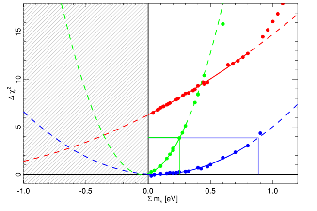
We construct the profile likelihood for $\sum m_{\nu}$. It is shown in Fig. 3 for the CMB, CMB+lensing and CMB+lensing+BAO data sets. We observe an intriguing feature with the CMB data set. Even though the parabolic fit of the profile likelihood is poor, the minimum lies at about $-2.5\sigma$ into the unphysical negative region. When adding the lensing trispectrum information, it shifts back to a value compatible with zero. We do not yet have a proper understanding of why this is happening, but note a possible connection to the $A_{\rm L}$ issue discussed in Planck Collaboration XVI (2013), where this phenomenological parameter is discrepant from unity by about $2\sigma$ using the CMB data set, but lowered to $1\sigma$ when adding the lensing information.

We can then understand why our previous argument on reducing the confidence interval by adding information is invalid near a physical boundary, even in a frequentist sense. If we consider a constant threshold of the profile likelihood (for instance around 8 on Fig. 3) we may end up with an upper limit that is smaller (even though the curvature is larger) when omitting the lensing information, because of the shift of the minimum into the unphysical region. This resembles the Bayesian result.

However the methodologies shows their differences in this situation. In the Bayesian case, when combining somewhat incompatible data sets within a model the credible region enlarges to account for it. In the frequentist case, thresholding the profile likelihood is incorrect and we apply instead the Feldman & Cousins (1998) prescription. Within this classical framework, there is a decoupling of the confidence level of the goodness of fit probability from the one used in building the confidence interval. Unlike in the Bayesian case, one first tests the consistency of the data with the model, and then constructs the confidence interval (at some given level) only for the candidates that fulfil it. In our case, a minimum at $-2.5\sigma$ is very unlikely (below 1% probability) and we will therefore not consider it in the following.

We give in Table 5 the parameters of the parabolic fits $\chi^{2}(\sum m_{\nu})=\chi^{2}_{\mathrm{min}}+\left[(\sum m_{\nu}-m_{0})/\sigma_{\nu}\right]^{2}$. We only use points within $2\sigma_{\nu}$ from zero, since the function is not necessarily quadratic far from its minimum. In the following we will vary this cut. We report here the numbers that lead to the largest final limit.

Data set Fitted range $$m_{0}$$

CMB+lensing

CMB+lensing+BAO

Table 5: Estimates of the minima positions ($m_{0}$) and curvature ($\sigma_{\nu}$) from the parabolic fits of Fig. 3 for the data sets including lensing. The range of points used corresponds roughly to $2\sigma$.

The classical Neyman construction of a confidence interval has some inherent degree of freedom in it (e.g., Beringer et al. 2012). The Feldman–Cousins prescription, that is most powerfull near a physical a boundary, is to introduce an ordering based upon the likelihood ratios $R$:

$$R=\frac{{\cal L}(x|\mu)}{{\cal L}(x|\mu_{\mathrm{best}})}\thinspace,$$ (4)

where $x$ is the measured value of the sum of neutrino masses $\sum m_{\nu}$, $\mu$ is the true value, and $\mu_{\mathrm{best}}$ is the best-fit value of $\sum m_{\nu}$, given the data and the physically-allowed region for $\mu$. Hence we have $\mu_{\mathrm{best}}=x$ if $x\geq 0$, but $\mu_{\mathrm{best}}=0$ if $x<0$, and the ratio $R$ is given by (Feldman & Cousins 1998):

$$\exp({-(x-\mu)^{2}/2}) \mathrm{for}\;x>0;$$ (5)

$$\exp({x\mu-{\mu^{2}/2}}) \mathrm{for}\;x\leq 0.$$ (6)

We then search for an interval $[x_{1},x_{2}]$ such that $R(x_{1})=R(x_{2})$ and

$$\int_{x_{1}}^{x_{2}}{\cal L}(x|\mu)dx=\alpha,$$ (7)

with $\alpha=0.95$ as the confidence level. These intervals are tabulated in Feldman & Cousins (1998).

We obtain the confidence interval $[\mu_{1},\mu_{2}]$ for each $x=m_{0}/\sigma_{\nu}$ extracted from the parabolic fit to the $\chi^{2}$ profile as given in Table 5. The upper limits are then simply $\mu_{2}\times\sigma_{\nu}$.

We give our final results in Table 6 and compare them to the Planck Bayesian ones of Planck Collaboration XVI (2013). The agreement is impressive, despite the use of two very different statistical techniques. Finally, we varied the range of points used in the parabolic fit and the limits we obtain are always lower than the one reported in Table 6, meaning that our results are conservative.

Data set Bayesian posterior profile likelihood

CMB+lensing $$0.85$$

CMB+lensing+BAO

Table 6: Upper limit (95% confidence) on the neutrino mass (in $\mathrm{\thinspace e\kern-1.00006ptV}$) in the Planck Bayesian framework and in the frequentist one based on Feldman–Cousins prescription.

5 Conclusion

The use of Bayesian methodology in cosmology is partly motivated by the fact that one observes a single realization of the Universe, while, in particle physics, one accumulates a number of events which leads more naturally to using frequentist methods. This argument is of a sociological rather than scientific nature, and nothing prevents us from using one or the other methodology in these fields.

We demonstrated that a purely frequentist method is tractable with the recent Planck-led high-precision cosmology data. It required lowering the numerical noise of the Boltzmann solver code and we have provided a set of precision parameters for the class software that, in conjunction with a proper Minuit minimization strategy, allowed us to perform the roughly $40$ parameter optimization efficiently. We re-determined the maximum likelihood solution, obtaining essentially consistent results but with a slightly better $\chi^{2}$ value.

We built profile likelihoods for each of the cosmological parameters of the $\Lambda$CDM model, using the CMB and CMB+BAO data sets, and obtained results very similar to those from the Bayesian methodology. This confirmed, in this model, that the Planck results do not depend on the choice of base parameters (implicit priors) and are free of volume effects in the likelihood projection during the marginalization process.

When including the neutrino mass as a free parameter, the profile likelihood helped us to understand why the computed upper limit increases when including the extra information from CMB lensing. This is not due to the Bayesian methodology, but is related to the physical boundary $\sum m_{\nu}>0$. The profile likelihood analysis showed that neutrino mass limits obtained without using the lensing information were pulled down to unphysical negative values. Including the extra CMB lensing information allowed us to obtain consistent frequentist results.

Using the Feldman–Cousins prescription, we obtained a 95% confidence upper limit of $\sum m_{\nu}\leq 0.26\mathrm{\thinspace e\kern-1.00006ptV}$ for the CMB+lensing+BAO combination, again in excellent agreement with the Bayesian result.

Appendix A Note on CPU time

It it sometimes stated that multi-dimensional minimization in high-dimension space is inefficient (or intractable) while MCMC methods scale linearly. Both statements need clarification.

Standard MCMC methods (e.g., Metropolis–Hastings or Gibbs sampling as in CosmoMC) are extremely CPU-intensive. They require the lengthy computation of a multi-variate proposal before running a final Markov chain, which by essence is sequential and therefore cannot scale on multiple processors. In the Planck case about ${\cal O}(10^{5})$ iterations (i.e., computations of the likelihood) were needed for this final stage.

One Minuit minimization in our scheme is obtained in about ${\cal O}(10^{4})$ iterations. It, however, requires a higher precision tuning of the Boltzmann solver, which enhances the computation time of each likelihood by about a factor two. In practice the minimum, in the $D=40$ case, is found in about 10 hours, and is limited by the Boltzmann computation speed. The profile likelihood approach requires many minimizations but these are independent of one another. The problem now scales with the number of computers, so that the total wall-clock time is still of the same order of magnitude on a reasonable computer cluster.

References

- Anderson et al. (2012) Anderson, L., Aubourg, E., Bailey, S., et al. 2012, MNRAS, 427, 3435, 1203.6594
- ATLAS Collaboration (2013) ATLAS Collaboration. 2013, Combined measurements of the mass and signal strength of the Higgs-like boson with the ATLAS detector using up to 25 fb-1 of proton-proton collision data, Tech. Rep. ATLAS-CONF-2013-014, CERN, Geneva
- Beringer et al. (2012) Beringer, J., Arguin, J. F., Barnett, R. M., et al. 2012, Phys. Rev. D, 86, 010001
- Beutler et al. (2011) Beutler, F., Blake, C., Colless, M., et al. 2011, MNRAS, 416, 3017, 1106.3366
- Blas et al. (2011) Blas, D., Lesgourgues, J., & Tram, T. 2011, J. Cosmology Astropart. Phys., 7, 34, 1104.2933
- Christensen et al. (2001) Christensen, N., Meyer, R., Knox, L., & Luey, B. 2001, Classical and Quantum Gravity, 18, 2677, arXiv:astro-ph/0103134
- Das et al. (2013) Das, S., Louis, T., Nolta, M. R., et al. 2013, ArXiv e-prints, 1301.1037
- Davidon & Laboratory (1959) Davidon, W. & Laboratory, A. N. 1959, Variable metric method for minimization, AEC research and development report (Argonne National Laboratory)
- Feldman & Cousins (1998) Feldman, G. J. & Cousins, R. D. 1998, Phys. Rev. D, 57, 3873, arXiv:physics/9711021
- Fletcher (1970) Fletcher, R. 1970, Comput. J., 317
- Gonzalez-Morales et al. (2011) Gonzalez-Morales, A. X., Poltis, R., Sherwin, B. D., & Verde, L. 2011, ArXiv e-prints, 1106.5052
- Hamann (2012) Hamann, J. 2012, J. Cosmology Astropart. Phys., 3, 21, 1110.4271
- Hamann et al. (2007) Hamann, J., Hannestad, S., Raffelt, G. G., & Wong, Y. Y. Y. 2007, J. Cosmology Astropart. Phys., 8, 21, 0705.0440
- James (2007) James, F. 2007, Statistical Methods in Experimental Physics (World Scientific)
- James & Roos (1975) James, F. & Roos, M. 1975, Comput. Phys. Commun., 10, 343
- Kosowsky et al. (2002) Kosowsky, A., Milosavljevic, M., & Jimenez, R. 2002, Phys. Rev. D, 66, 063007, arXiv:astro-ph/0206014
- Lesgourgues (2011a) Lesgourgues, J. 2011a, ArXiv e-prints, 1104.2932
- Lesgourgues (2011b) Lesgourgues, J. 2011b, ArXiv e-prints, 1104.2934
- Lesgourgues et al. (2013) Lesgourgues, J., Mangano, G., Miele, G., & Pastor, S. 2013, Neutrino Cosmology (Cambridge: Cambridge Univ. Press)
- Lewis (2008) Lewis, A. 2008, Phys. Rev. D, 78, 023002
- Lewis & Bridle (2002) Lewis, A. & Bridle, S. 2002, Phys. Rev. D, 66, 103511, arXiv:astro-ph/0205436
- Padmanabhan et al. (2012) Padmanabhan, N., Xu, X., Eisenstein, D. J., et al. 2012, MNRAS, 427, 2132, 1202.0090
- Planck Coll. XVI (2013) Planck Coll. XVI. 2013, ArXiv e-prints, 1303.5076
- Planck Collaboration I (2013) Planck Collaboration I. 2013, Submitted to A&A, [arXiv:astro-ph/1303.5062]
- Planck Collaboration XV (2013) Planck Collaboration XV. 2013, Submitted to A&A, [arXiv:astro-ph/1303.5075]
- Planck Collaboration XVI (2013) Planck Collaboration XVI. 2013, Submitted to A&A, [arXiv:astro-ph/1303.5076]
- Planck Collaboration XVII (2013) Planck Collaboration XVII. 2013, Submitted to A&A, [arXiv:astro-ph/1303.5077]
- Reichardt et al. (2012) Reichardt, C. L., de Putter, R., Zahn, O., & Hou, Z. 2012, ApJ, 749, L9, 1110.5328
- Reid et al. (2010) Reid, B. A., Verde, L., Jimenez, R., & Mena, O. 2010, J. Cosmology Astropart. Phys., 1, 3, 0910.0008
- Wilks (1938) Wilks, A. S. S. 1938, Ann.Math.Statist., 1, 60
- Yèche et al. (2006) Yèche, C., Ealet, A., Réfrégier, A., et al. 2006, A&A, 448, 831, arXiv:astro-ph/0507170