Positivity and Boundedness Preserving Schemes for Space-Time Fractional Predator-Prey Reaction-Diffusion Model

Abstract.

The semi-implicit schemes for the nonlinear predator-prey reaction-diffusion model with the space-time fractional derivatives are discussed, where the space fractional derivative is discretized by the fractional centered difference and WSGD scheme. The stability and convergence of the semi-implicit schemes are analyzed in the $L_{\infty}$ norm. We theoretically prove that the numerical schemes are stable and convergent without the restriction on the ratio of space and time stepsizes and numerically further confirm that the schemes have first order convergence in time and second order convergence in space. Then we discuss the positivity and boundedness properties of the analytical solutions of the discussed model, and show that the numerical solutions preserve the positivity and boundedness. The numerical example is also presented.

School of Mathematics and Statistics, Lanzhou University,

Lanzhou, 730000, People’s Republic of China

1. Introduction

The predator-prey model, also known as the Lotka-Volterra equation, is a pair of first-order nonlinear ordinary differential equations frequently used to describe the dynamics of biological system in which two species interact, one as the predator and the other as prey [1]; and the unknown variables usually denote certain measure of total population. To interpret the unknown variables as spacial densities so as to allow the population size to vary throughout the considered region, Conway and Smoller introduce diffusion terms to the predator-prey model which allows diffusing as well as interacting each other [2]; and then the predator-prey reaction-diffusion model is obtained. With the development of the predator-prey model, it seems nature to introduce diffusion terms to the corresponding model, e.g., the Michaelis-Menten-Holling predator-prey reaction-diffusion model [3, 4]; and more general other models [5, 6, 7, 8].

Anomalous diffusion, including subdiffusion and superdiffuion, is also a diffusion process, but its mean squared displacement (MSD) is nonlinear with respect to time $t$, in contract to the classical diffusion process, in which the MSD is linear [9]; nowadays, it is widely recognized that the anomalous diffusion is ubiquitous, e.g., diffusion through porous media, protein diffusion within cells, and also being found in many other biological systems. So it seems reasonable/nature to introduce the anomalous diffusion to the predator-prey model. The subdiffusion is introduced to the Michaelis-Menten-Holling predator-prey model in [10] to get a new model; it is proved that the solution of the model is positive and bounded; and the numerical schemes preserving the positivity and boundedness are detailedly discussed. Here we introduce both the subdiffusion and superdiffusion to the Michaelis-Menten-Holling predator-prey model, and the system can be written as

$$\begin{array}[]{llll}\displaystyle\frac{\partial^{\alpha}N}{\partial t^{\alpha}}&=&D_{1}\displaystyle\frac{\partial^{\beta}N}{\partial|x|^{\beta}}+N\left(1-N-\frac{\varrho P}{P+N}\right),&x\in(l,r),\,\,t>0,\\ \\ \displaystyle\frac{\partial^{\alpha}P}{\partial t^{\alpha}}&=&D_{2}\displaystyle\frac{\partial^{\beta}P}{\partial|x|^{\beta}}+\sigma P\left(-\frac{\gamma+\kappa\delta P}{1+\kappa P}+\frac{N}{P+N}\right),&x\in(l,r),\,\,t>0,\end{array}$$ (1)

with the Caputo derivative in time and Riesz space fractional derivetive, where $\varrho$, $\sigma$ and $\kappa$ are positive real numbers and $N$ and $P$ denote the population densities of prey and predator respectively. Based on the practical applications, we are interested in the solutions of (1) with the nonnegative initial conditions

$$N(x,0)=g_{1}(x)\geq 0,~{}~{}~{}P(x,0)=g_{2}(x)\geq 0,~{}~{}~{}x\in(l,r),$$ (2)

and the homogeneous Neumann boundary conditions

$$(\partial{N(x,t)}/\partial x)|_{x=l\rm{~{}and~{}}r,\rm{~{}respectively}}=(\partial{P(x,t)}/\partial x)|_{x=l\rm{~{}and~{}}r,\rm{~{}respectively}}=0.$$ (3)

The positive constants $\gamma$ and $\delta$ in the coupled equations denote the minimal mortality and the limiting mortality of the predator, respectively. Throughout the paper, we assume that $\gamma$ satisfies the natural condition $0<\gamma\leq\delta$ and consider the case of the diffusion constants $D_{i}>0,\,i=1,2$.

The numerical methods for solving fractional partial differential equations are developing fast; most of them focus on fractional diffusion equations, including the space fractional diffusion equation [11, 12] and the time fractional diffusion equation [13, 14, 15, 16, 17, 18]. Because of the stability issue, the space fractional derivative is usually approximated by the shifted Grünwald-Letnikov definition with the finite stepsize; and the truncation error is first-order. Recently, the second-order discretizations for space fractional derivative appear: based on the so-called “fractional centered difference”, Ortigueira gets the second-order approximation for the Riesz fractional derivative [19], and its applications can be seen in [20, 21]; Tian et al obtain the so-called WSGD second order approximation for both the left and right Riemann-Liouville derivatives [22], and its compact version has third-order accuracy [23].

This paper first proves that the analytical solutions of the space-time fractional predator-prey reaction-diffusion model (1)-(3) are positive and bounded; and then designs the numerical schemes to solve it. The space fractional derivative is discretized by the fractional centered difference [19] and the WSGD operators [22], respectively. We prove that both the two obtained schemes have second-order accuracy in space and preserve the positivity and boundedness of the analytical solutions. In particular, the stability of the numerical scheme without the restriction on the ratio of the space and time stepsizes is also strictly proved. And the numerical example is provided to confirm the theoretical results.

The outline of this paper is as follows. In Section 2, we present two finite difference schemes for the space-time fractional predator-prey reaction-diffusion model. The detailed discussions on the stability and convergence with first-order in time and second-order in space are given in Section 3. In Section 4, we prove that the analytical solutions of the discussed model are positive and bounded; and the provided two schemes preserve the positivity and boundedness. The numerical experiments to confirm the convergent orders and the positivity and boundedness preserving are performed in Section 5. And we conclude the paper with some discussions in the last section.

2. Numerical schemes for the space-time fractional predator-prey reaction-diffusion model

As mentioned in the introduction section, the model we discuss is as follows:

$$\begin{array}[]{llll}\displaystyle\frac{\partial^{\alpha}N}{\partial t^{\alpha}}&=&D_{1}\displaystyle\frac{\partial^{\beta}N}{\partial|x|^{\beta}}+N\left(1-N-\frac{\varrho P}{P+N}\right),&x\in(l,r),\,\,0<t\leq T,\\ \\ \displaystyle\frac{\partial^{\alpha}P}{\partial t^{\alpha}}&=&D_{2}\displaystyle\frac{\partial^{\beta}P}{\partial|x|^{\beta}}+\sigma P\left(-\frac{\gamma+\kappa\delta P}{1+\kappa P}+\frac{N}{P+N}\right),&x\in(l,r),\,\,0<t\leq T,\end{array}$$ (4)

with $0<\alpha<1$, $1<\beta<2$, and use the following initial conditions

$$N(x,0)=g_{1}(x),\,P(x,0)=g_{2}(x),\qquad x\in[l,r]$$ (5)

and the homogeneous boundary conditions

$$\frac{\partial{N(x,t)}}{\partial x}|_{x=l}=\frac{\partial{N(x,t)}}{\partial x}|_{x=r}=\frac{\partial{P(x,t)}}{\partial x}|_{x=l}=\frac{\partial{P(x,t)}}{\partial x}|_{x=r}=0,\quad 0<t\leq T.\\ \\$$ (6)

In (4), the time fractional operator $\frac{\partial^{\alpha}u(x,t)}{\partial t^{\alpha}}$ denotes the Caputo fractional derivative

$$\frac{\partial^{\alpha}u(x,t)}{\partial x^{\alpha}}=\frac{1}{\Gamma(1-\alpha)}\int^{t}_{0}\frac{\partial u(x,s)}{\partial s}\frac{1}{(t-s)^{\alpha}}ds,$$

and $\frac{\partial^{\beta}u}{\partial|x|^{\beta}}$ denotes the Riesz fractional derivative

$$\frac{\partial^{\beta}u(x,t)}{\partial|x|^{\beta}}=-\frac{1}{2cos(\beta\pi/2)\Gamma(2-\beta)}\frac{d^{2}}{dx^{2}}\int^{r}_{l}|x-\xi|^{1-\beta}u(\xi,t)d\xi.$$ (7)

For ease of presentation, we uniformly divide the spacial domain $[l,r]$ into $M$ subintervals with stepsize $h$ ($=(r-l)/M$) and the time domain $[0,T]$ into $N$ subintervals with steplength $\tau$ ($=T/N$). Let $x_{i}=l+ih\,(i=0,1,\cdots,M)$, $t_{k}=k\tau\,(k=0,1,\cdots,N)$, and denote the grid function as $u^{k}_{i}=u(x_{i},t_{k})$. We use the discrete scheme of the Caputo derivative in the following form [16]

$$D^{\alpha}_{\tau}u_{i}^{k}=\frac{\tau^{-\alpha}}{\Gamma(2-\alpha)}\big{[}u_{i}^{k}-\sum^{k-1}_{n=1}(b_{k-n-1}-b_{k-n})u_{i}^{n}-b_{k-1}u_{i}^{0}\big{]},$$ (8)

where $b_{n}=(n+1)^{1-\alpha}-n^{1-\alpha}>0$, and $1=b_{0}>b_{1}>\cdots>b_{k-1}>(1-\alpha)k^{-\alpha}$. Note that the above discrete scheme has $2-\alpha$ order accuracy in time, i.e.,

$$\frac{\partial^{\alpha}u(x_{i},t)}{\partial t^{\alpha}}\big{|}_{t=t_{k}}=D^{\alpha}_{\tau}u_{i}^{k}+\mathcal{O}(\tau^{2-\alpha}).$$ (9)

For the Riesz space fractional derivative, we introduce two second order finite difference approximation schemes (fractional centered difference scheme and second order WSGD scheme) in the next parts.

2.1. Fractional centered difference scheme

In this part, we use the fractional centered difference [19] to discretize the spatial factional derivative. The Riesz fractional derivative can be redefined as

$$\frac{\partial^{\beta}u(x,t)}{\partial|x|^{\beta}}=\lim_{h\rightarrow 0}\left(-\frac{1}{h^{\beta}}\sum_{j=[(l-r+x)/h]}^{[x/h]}\frac{(-1)^{j}\Gamma(\beta+1)}{\Gamma(\frac{\beta}{2}-j+1)\Gamma(\frac{\beta}{2}+j+1)}u(x-jh,t)\right).$$ (10)

Denoting the weights as

$$g_{j}=\frac{(-1)^{j}\Gamma(\beta+1)}{\Gamma(\frac{\beta}{2}-j+1)\Gamma(\frac{\beta}{2}+j+1)},$$

we get the fractional centered difference approximation for the Riesz fractional derivative

$$\delta_{x}^{\beta}u_{i}^{k}=-\frac{1}{h^{\beta}}\sum_{j=-M+i}^{i}g_{j}u_{i-j}^{k},$$ (11)

where the weights $g_{j}$ satisfy the following properties:

1. $g_{0}\geq 0$,

2. $g_{-j}=g_{j}\leq 0$,

3. $g_{j+1}=\left(1-\frac{\beta+1}{\beta/2+j+1}\right)g_{j}$, and $|g_{j+1}|<|g_{j}|$,

4. $\sum\limits_{j=-\infty}^{\infty}g_{j}=0$, and $\sum\limits_{j=-M+i\atop j\neq 0}^{i}|g_{j}|<g_{0}$.

From [20], we know that the accuracy of fractional centered difference approximation is as,

Lemma 2.1.

If $u(x,t_{i})\in\mathcal{C}^{5}[l,r]$, then we have

$$\frac{\partial^{\beta}u(x,t_{i})}{\partial|x|^{\beta}}|_{x=x_{i}}=\delta_{x}^{\beta}u_{i}^{k}+\mathcal{O}(h^{2}),$$

with $1<\beta<2$.

If the fractional centered difference approximation is substituted into the system of reaction-diffusion equation (4), then the resulting semi-implicit finite difference scheme is

$$\begin{array}[]{llll}\displaystyle D^{\alpha}_{\tau}N_{i}^{k+1}&=&D_{1}\displaystyle\delta_{x}^{\beta}N_{i}^{k+1}+N_{i}^{k}\left(1-N_{i}^{k}-\frac{\varrho P_{i}^{k}}{P_{i}^{k}+N_{i}^{k}}\right),\\ \\ \displaystyle D^{\alpha}_{\tau}P_{i}^{k+1}&=&D_{2}\displaystyle\delta_{x}^{\beta}P_{i}^{k+1}+\sigma P_{i}^{k}\left(-\frac{\gamma+\kappa\delta P_{i}^{k}}{1+\kappa P_{i}^{k}}+\frac{N_{i}^{k}}{P_{i}^{k}+N_{i}^{k}}\right),\end{array}$$ (12)

with initial conditions

$$N_{i}^{0}=g_{1}(x_{i}),\,P_{i}^{0}=g_{2}(x_{i}).$$ (13)

For guaranteeing the second-order accuracy in space, we give the three point interpolation scheme for the Neumann boundary conditions:

$$\begin{array}[]{llll}\quad\quad\quad N_{2}^{k}-4N_{1}^{k}+3N_{0}^{k}&=0,\displaystyle&P_{2}^{k}-4P_{1}^{k}+3P_{0}^{k}=0,\quad 0\leq k\leq N,\\ \\ N_{M-2}^{k}-4N_{M-1}^{k}+3N_{M}^{k}&=0,\displaystyle&P_{M-2}^{k}-4P_{M-1}^{k}+3P_{M}^{k}=0,\quad 0\leq k\leq N.\end{array}$$ (14)

Eq. (12)-(14) may be rearranged and written as matrix form and solved to get the numerical solution at the time step $t_{k+1}$:

$$(I+A_{1})N^{k+1} =\sum_{j=1}^{k}(b_{j}-b_{j+1})N^{k-j}+b_{k}N^{0}+\mu N^{k}\left(1-N^{k}-\frac{\varrho P^{k}}{P^{k}+N^{k}}\right),$$

$$(I+A_{2})P^{k+1} =\sum_{j=1}^{k}(b_{j}-b_{j+1})P^{k-j}+b_{k}P^{0}+\mu\sigma P^{k}\left(-\frac{\gamma+\kappa\delta P^{k}}{1+\kappa P^{k}}+\frac{N^{k}}{P^{k}+N^{k}}\right),$$

where $N^{k}=(N_{1}^{k},N_{2}^{k},\cdots,N_{M-1}^{k})$, $P^{k}=(P_{1}^{k},P_{2}^{k},\cdots,P_{M-1}^{k})$ and $A_{i}$ is a $(M-1)\times(M-1)$ square matrix

$$A_{i}=\frac{\mu D_{i}}{h^{\beta}}\left(\begin{array}[]{ccccc}g_{0}+\frac{4}{3}g_{1}&g_{-1}-\frac{1}{3}g_{1}&g_{-2}&\cdots&g_{-M+2}+\frac{4}{3}g_{-M+1}\\ g_{1}+\frac{4}{3}g_{2}&g_{0}-\frac{1}{3}g_{2}&g_{-1}&&g_{-M+3}+\frac{4}{3}g_{-M+2}\\ \vdots&&&\ddots&\\ g_{M-2}+\frac{4}{3}g_{M-1}&g_{M-3}-\frac{1}{3}g_{M-1}&g_{M-4}&&g_{0}+\frac{4}{3}g_{-1}\\ \end{array}\right).$$ (15)

2.2. Second order WSGD scheme

The other equivalent definition of the Riesz fractional derivative $\frac{\partial^{\beta}u(x,t)}{\partial|x|^{\beta}}$ is

$$\frac{\partial^{\beta}u(x,t)}{\partial|x|^{\beta}}=\frac{-1}{2cos(\beta\pi/2)}(_{l}D_{x}^{\beta}u(x,t)+_{x}D_{r}^{\beta}u(x,t)),$$ (16)

where ${}_{l}D_{x}^{\beta}u(x,t)$ and ${}_{x}D_{r}^{\beta}u(x,t)$ denote the left and right Riemann-Liouville fractional derivatives of the function $u(x,t)$, respectively. According to the discussions of [22], we present the discrete approximations of the left and right Riemann-Liouville fractional derivatives as follows:

$$\begin{array}[]{c}{}_{l}D^{\beta}_{x}u(x_{i})=\frac{1}{h^{\beta}}\sum_{j=0}^{i+1}w_{j}u(x_{i-j+1})+\mathcal{O}(h^{2}),\\ \\ {}_{x}D^{\beta}_{r}u(x_{i})=\frac{1}{h^{\beta}}\sum_{j=0}^{M-i+1}w_{j}u(x_{i+j-1})+\mathcal{O}(h^{2}),\end{array}$$ (17)

where $w_{0}=\alpha/2$, $w_{j}=\Gamma(j-\beta-1)/(\Gamma(-\beta)\Gamma(j))\cdot(1-(\beta/2)\cdot(\beta+1)/j)$. After substituting (17) into (16) and merging the same terms, we get the discrete approximation of the Riesz fractional derivative

$$\delta_{x}u_{i}^{k}=\frac{-1}{h^{\beta}}\sum_{j=-M+i}^{i}\theta_{j}u_{i-j}^{k},$$

where the weights $\theta_{j}$ satisfy the following properties

1. $\theta_{0}=\frac{w_{1}}{cos(\beta\pi/2)}=\frac{2-\beta-\beta^{2}}{2cos(\beta\pi/2)}>0$,
   
   

2. $\theta_{1}=\theta_{-1}=\frac{w_{0}+w_{2}}{2cos(\beta\pi/2)}=\frac{\beta(\beta+2)(\beta-1)}{8cos(\beta\pi/2)}<0$, 
   
   for $|j|>1$, $\theta_{j}=\theta_{-j}=\frac{w_{j+1}}{2cos(\beta\pi/2)}=\frac{\Gamma(j-\beta)}{2cos(\beta\pi/2)\Gamma(-\beta)\Gamma(j+1)}\left(1-\frac{\beta(\beta+1)}{2(j+1)}\right)\leq 0$,
   
   

3. $\theta_{j+1}=\frac{(-\beta+j)(\beta+\beta^{2}-2(2+j))}{(2+j)(\beta+\beta^{2}-2(1+j))}\theta_{j}$, for $|j|\geq 2$, and $|\theta_{1}|>|\theta_{2}|\geq|\theta_{3}|\geq\cdots$,
   
   

4. $\sum\limits_{j=-\infty}^{\infty}\theta_{j}=0$, and $\sum\limits_{j=-M+i\atop j\neq 0}^{i}|\theta_{j}|<\theta_{0}$.

In view of the approximations (17), we know that the above discrete scheme of the Riesz fractional derivative also has second-order accuracy

$$\frac{\partial^{\beta}u(x,t)}{\partial|x|^{\beta}}\big{|}_{x=x_{k},t=t_{j}}=\frac{-1}{h^{\beta}}\sum_{j=-M+i}^{i}\theta_{j}u_{i-j}^{k}+\mathcal{O}(h^{2}).$$ (18)

If the second-order WSGD discretization is substituted into the reaction-diffusion equations (4), we obtain the new semi-implicit WSGD finite difference scheme. And the same initial and boundary discretizations (13) and (14) are used. Then we can get the same formulations for the WSGD scheme as the ones for the fractional centered difference scheme (12)-(15).

The semi-implicit fractional centered difference and the semi-implicit WSGD scheme have the same structure, and in particular, their discretized weights have the similar properties. So in the following, the two schemes have the same analyses, and we just focus on the first scheme.

3. Stability and convergence of the numerical schemes

Now we first denote the two nonlinear terms by

$$f_{1}(N,P)=N\left(1-N-\frac{\varrho P}{P+N}\right)$$ (19)

and

$$f_{2}(N,P)=\sigma P\left(-\frac{\gamma+\kappa\delta P}{1+\kappa P}+\frac{N}{P+N}\right)$$ (20)

for convenience. And assume that they satisfy local Lipschitz condition, i.e., there exists a positive constant $L$ such that

$$|f_{1}(N_{1},P_{1})-f_{1}(N_{2},P_{2})|\leq L(|N_{1}-N_{2}|+|P_{1}-P_{2}|)$$

and

$$|f_{2}(N_{1},P_{1})-f_{2}(N_{2},P_{2})|\leq L(|N_{1}-N_{2}|+|P_{1}-P_{2}|),$$

when $|N_{1}-N_{2}|\leq\epsilon_{0}$ and $|P_{1}-P_{2}|\leq\epsilon_{0}$ for a given positive constant $\epsilon_{0}$. Then the discrete scheme (12) can be rewritten as the following form

$$\left(\frac{1}{\mu}+\frac{D_{1}g_{0}}{h^{\beta}}\right)N_{i}^{k+1}= \frac{1}{\mu}\sum_{n=1}^{k}(b_{k-n}-b_{k-n+1})N_{i}^{n}+\frac{1}{\mu}b_{k}N_{i}^{0}$$ (21)

$$-\frac{D_{1}}{h^{\beta}}\sum_{j=-M+i\atop j\neq 0}^{i}g_{j}N_{i-j}^{k+1}+f_{1}(N_{i}^{k},P_{i}^{k}),$$

$$\left(\frac{1}{\mu}+\frac{D_{2}g_{0}}{h^{\beta}}\right)P_{i}^{k+1}= \frac{1}{\mu}\sum_{n=1}^{k}(b_{k-n}-b_{k-n+1})P_{i}^{n}+\frac{1}{\mu}b_{k}P_{i}^{0}$$

$$-\frac{D_{2}}{h^{\beta}}\sum_{j=-M+i\atop j\neq 0}^{i}g_{j}P_{i-j}^{k+1}+f_{2}(N_{i}^{k},P_{i}^{k}),$$

where $\mu=\Gamma(2-\alpha)\tau^{\alpha}$. In this paper, we use $L_{\infty}$ norm of $\{u_{i}^{k}\}_{i=1}^{M-1}$ which is defined as

$$\|u^{k}\|=\max_{1\leq i\leq M-1}|u^{k}_{i}|.$$

Let $(\bar{N}_{i}^{k},\bar{P}_{i}^{k})$ be the approximate solution to the numerical scheme and denote $\epsilon_{i}^{k}=N_{i}^{k}-\bar{N}_{i}^{k}$ and $\varepsilon_{i}^{k}=P_{i}^{k}-\bar{P}_{i}^{k}$. Then under the small perturbations, there exists the following numerical stability result.

Theorem 3.1.

The numerical schemes (12)-(14) are stable and there exist

$$\begin{array}[]{llll}\displaystyle\|\epsilon^{k}\|\leq\frac{1}{(1-\alpha)-T^{\alpha}\Gamma(2-\alpha)L}(\|\epsilon^{0}\|+\|\varepsilon^{0}\|),\\ \\ \displaystyle\|\varepsilon^{k}\|\leq\frac{1}{(1-\alpha)-T^{\alpha}\Gamma(2-\alpha)L}(\|\epsilon^{0}\|+\|\varepsilon^{0}\|),\end{array}$$ (22)

when $T<(1/(\Gamma(1-\alpha)L))^{1/\alpha}$.

Proof.

We prove this theorem by mathematical induction. Using the first equation of (21), we have

$$\left(\frac{1}{\mu}+\frac{D_{1}g_{0}}{h^{\beta}}\right)\epsilon_{i}^{k+1}= \frac{1}{\mu}\sum_{n=1}^{k}(b_{k-n}-b_{k-n+1})\epsilon_{i}^{n}+\frac{1}{\mu}b_{k}\epsilon_{i}^{0}$$

$$-\frac{D_{1}}{h^{\beta}}\sum_{j=-M+i\atop j\neq 0}^{i}g_{j}\epsilon_{i-j}^{k+1}+(f_{1}(N_{i}^{k},P_{i}^{k})-f_{1}(\bar{N}_{i}^{k},\bar{P}_{i}^{k})).$$

According to the numerical approximations (14), when $i\neq 2,M-2$, the above equation can be rewritten as

$$\left(\frac{1}{\mu}+\frac{D_{1}g_{0}}{h^{\beta}}\right)\epsilon_{i}^{k+1}= \frac{1}{\mu}\sum_{n=1}^{k}(b_{k-n}-b_{k-n+1})\epsilon_{i}^{n}+\frac{1}{\mu}b_{k}\epsilon_{i}^{0}-\frac{D_{1}}{h^{\beta}}\sum_{j=-M+i+1\atop j\neq 0}^{i-1}g_{j}\epsilon_{i-j}^{k+1}$$

$$+\frac{D_{1}}{3h^{\beta}}(g_{i}\epsilon_{2}^{k+1}+g_{-M+i}\epsilon_{M-2}^{k+1})-\frac{4D_{1}}{3h^{\beta}}(g_{i}\epsilon_{1}^{k+1}+g_{-M+i}\epsilon_{M-1}^{k+1})$$

$$+(f_{1}(N_{i}^{k},P_{i}^{k})-f_{1}(\bar{N}_{i}^{k},\bar{P}_{i}^{k}))$$

$$= \frac{1}{\mu}\sum_{n=1}^{k}(b_{k-n}-b_{k-n+1})\epsilon_{i}^{n}+\frac{1}{\mu}b_{k}\epsilon_{i}^{0}-\frac{D_{1}}{h^{\beta}}\sum_{j=-M+i+1\atop j\neq 0,i-2,-M+i+2}^{i-1}g_{j}\epsilon_{i-j}^{k+1}$$

$$+\frac{D_{1}}{h^{\beta}}((g_{i}/3-g_{i-2})\epsilon_{2}^{k+1}+(g_{-M+i}/3-g_{-M+i+2})\epsilon_{M-2}^{k+1})$$

$$-\frac{4D_{1}}{3h^{\beta}}(g_{i}\epsilon_{1}^{k+1}+g_{-M+i}\epsilon_{M-1}^{k+1})+(f_{1}(N_{i}^{k},P_{i}^{k})-f_{1}(\bar{N}_{i}^{k},\bar{P}_{i}^{k})).$$

Since $g_{i}/3-g_{i-2}>0$ and $g_{-M+i}/3-g_{-M+i+2}>0$, we get

$$\left(\frac{1}{\mu}+\frac{D_{1}g_{0}}{h^{\beta}}\right)\|\epsilon_{i}^{k+1}\|$$

$$\leq \frac{1}{\mu}\sum_{n=1}^{k}(b_{k-n}-b_{k-n+1})\|\epsilon_{i}^{n}\|+\frac{1}{\mu}b_{k}\|\epsilon_{i}^{0}\|-\frac{D_{1}}{h^{\beta}}\sum_{j=-M+i+1\atop j\neq 0,i-2,-M+i+2}^{i-1}g_{j}\|\epsilon_{i-j}^{k+1}\|$$

$$+\frac{D_{1}}{h^{\beta}}((g_{i}/3-g_{i-2})\|\epsilon_{2}^{k+1}\|+(g_{-M+i}/3-g_{-M+i+2})\|\epsilon_{M-2}^{k+1}\|)$$

$$-\frac{4D_{1}}{3h^{\beta}}(g_{i}\|\epsilon_{1}^{k+1}\|+g_{-M+i}\|\epsilon_{M-1}^{k+1}\|)+L(\|N_{i}^{k}-\bar{N}_{i}^{k}\|+\|P_{i}^{k}-\bar{P}_{i}^{k}\|).$$

From the above inequality we know that

$$\left(\frac{1}{\mu}+\frac{D_{1}g_{0}}{h^{\beta}}\right)\|\epsilon^{k+1}\|\leq \frac{1}{\mu}\sum_{n=1}^{k}(b_{k-n}-b_{k-n+1})\|\epsilon^{n}\|+\frac{1}{\mu}b_{k}\|\epsilon^{0}\|+L(\|\epsilon^{k}\|+\|\varepsilon^{k}\|)$$

$$-\frac{D_{1}}{h^{\beta}}\sum_{j=-M+i\atop j\neq 0}^{i}g_{j}\|\epsilon^{k+1}\|.$$

Together with the fourth property of coefficient $g_{i}$, we can obtain the following inequality

$$\left(\frac{1}{\mu}+\frac{D_{1}g_{0}}{h^{\beta}}\right)\|\epsilon^{k+1}\|\leq \frac{1}{\mu}\sum_{n=1}^{k}(b_{k-n}-b_{k-n+1})\|\epsilon^{n}\|+\frac{1}{\mu}b_{k}\|\epsilon^{0}\|+\frac{D_{1}g_{0}}{h^{\beta}}\|\epsilon^{k+1}\|$$

$$+L(\|\epsilon^{k}\|+\|\varepsilon^{k}\|).$$

Therefore,

$$\|\epsilon^{k+1}\|\leq\sum_{n=1}^{k}(b_{k-n}-b_{k-n+1})\|\epsilon^{n}\|+b_{k}\|\epsilon^{0}\|+L\mu(\|\epsilon^{k}\|+\|\varepsilon^{k}\|).$$ (23)

When $i=2$, we have

$$\left(\frac{1}{\mu}+\frac{D_{1}g_{0}}{h^{\beta}}\right)\epsilon_{2}^{k+1}-\frac{D_{1}}{h^{\beta}}g_{2}/3\epsilon_{2}^{k+1}$$

$$= \frac{1}{\mu}\sum_{n=1}^{k}(b_{k-n}-b_{k-n+1})\epsilon_{2}^{n}+\frac{1}{\mu}b_{k}\epsilon_{2}^{0}-\frac{D_{1}}{h^{\beta}}\sum_{j=-M+3\atop j\neq 0,-M+4}^{1}g_{j}\epsilon_{2-j}^{k+1}$$

$$+\frac{D_{1}}{h^{\beta}}(g_{-M+2}/3-g_{-M+4})\epsilon_{M-2}^{k+1}$$

$$-\frac{4D_{1}}{3h^{\beta}}(g_{2}\epsilon_{1}^{k+1}+g_{-M+2}\epsilon_{M-1}^{k+1})+(f_{1}(N_{2}^{k},P_{2}^{k})-f_{1}(\bar{N}_{2}^{k},\bar{P}_{2}^{k})).$$

Then in the similar way as above, we can also get the estimate (23) for $i=2$. If $i=M-2$, there exists a similar argument.

By almost the same deduction as $\|\epsilon^{k+1}\|$, we can get

$$\|\varepsilon^{k+1}\|\leq\sum_{n=1}^{k}(b_{k-n}-b_{k-n+1})\|\varepsilon^{n}\|+b_{k}\|\varepsilon^{0}\|+L\mu(\|\epsilon^{k}\|+\|\varepsilon^{k}\|).$$ (24)

For $k=1$, it’s easy to check that (22) holds. When $k>1$, suppose (22) holds for $n=1,\cdots,k$. Then there exists

$$\|\epsilon^{k+1}\|\leq\displaystyle\left(\frac{1-b_{k}+2L\mu}{(1-\alpha)-T^{\alpha}\Gamma(2-\alpha)L}+b_{k}\right)(\|\epsilon^{0}\|+\|\varepsilon^{0}\|).$$

We just need to prove

$$1-b_{k}+2L\mu+b_{k}((1-\alpha)-T^{\alpha}\Gamma(2-\alpha)L)\leq 1,$$

i.e.,

$$2L\mu\cdot b_{k}^{-1}\leq\alpha+T^{\alpha}\Gamma(2-\alpha)L.$$

Using $\mu=\Gamma(2-\alpha)\tau^{\alpha}=\Gamma(2-\alpha)\frac{T^{\alpha}}{N^{\alpha}}$, $b_{k}^{-1}<\frac{(k+1)^{\alpha}}{1-\alpha}$ and $\Gamma(1-\alpha)T^{\alpha}L<1$, we can obtain

$$2L\mu\cdot b_{k}^{-1}<2L\cdot\Gamma(2-\alpha)\frac{T^{\alpha}}{N^{\alpha}}\cdot\frac{(k+1)^{\alpha}}{1-\alpha}\leq 2L\cdot\Gamma(1-\alpha)T^{\alpha},$$

and

$$\alpha+T^{\alpha}\Gamma(2-\alpha)L>2L\cdot\Gamma(1-\alpha)T^{\alpha}.$$

This implies that

$$1-b_{k}+2L\mu+b_{k}((1-\alpha)-T^{\alpha}\Gamma(2-\alpha)L)\leq 1.$$

So

$$\|\epsilon^{k+1}\|\leq\displaystyle\frac{1}{(1-\alpha)-T^{\alpha}\Gamma(2-\alpha)L}(\|\epsilon^{0}\|+\|\varepsilon^{0}\|),$$

and

$$\|\varepsilon^{k+1}\|\leq\displaystyle\frac{1}{(1-\alpha)-T^{\alpha}\Gamma(2-\alpha)L}(\|\epsilon^{0}\|+\|\varepsilon^{0}\|).$$

∎

Theorem 3.2.

Let $\{(N(x_{i},t_{k}),P(x_{i},t_{k}))\}_{i=1}^{M-1}$ and $\{(N_{i}^{k},P_{i}^{k})\}_{i=1}^{M-1}$ be the exact solutions of the subdiffusive reaction-diffusion equation (4)-(6) and of the numerical schemes (12)-(14) respectively and define $\rho_{i}^{k}=N(x_{i},t_{k})-N_{i}^{k}$ and $\eta_{i}^{k}=P(x_{i},t_{k})-P_{i}^{k}$. Then $\rho^{k}$ and $\eta^{k}$ satisfy the following error estimates:

$$\|\rho^{n}\|\leq C(\tau+h^{2})\,and\,\|\eta^{n}\|\leq C(\tau+h^{2}),$$ (25)

when $T<(1/(\Gamma(1-\alpha)L))^{1/\alpha}$.

Proof.

According to the first equation of (21), when $i\neq 2,M-2$, we can get the following inequality

$$\left(\frac{1}{\mu}+\frac{D_{1}g_{0}}{h^{\beta}}\right)|\rho_{i}^{k+1}|$$

$$\leq \frac{1}{\mu}\sum_{n=1}^{k}(b_{k-n}-b_{k-n+1})|\rho_{i}^{n}|+\frac{1}{\mu}b_{k}|\rho_{i}^{0}|-\frac{D_{1}}{h^{\beta}}\sum_{j=-M+i+1\atop j\neq 0,i-2,-M+i+2}^{i-1}g_{j}|\rho_{i-j}^{k+1}|$$

$$+\frac{D_{1}}{h^{\beta}}((g_{i}/3-g_{i-2})|\rho_{2}^{k+1}|+(g_{-M+i}/3-g_{-M+i+2})|\rho_{M-2}^{k+1}|)$$

$$-\frac{4D_{1}}{3h^{\beta}}(g_{i}|\rho_{1}^{k+1}|+g_{-M+i}|\rho_{M-1}^{k+1}|)+L(|\rho_{i}^{k}|+|\eta_{i}^{k}|)+r_{1i}^{k+1},$$

where $r_{1}^{k+1}=O(\tau+h^{2})$. From the above inequality we know that

$$\left(\frac{1}{\mu}+\frac{D_{1}g_{0}}{h^{\beta}}\right)\|\rho^{k+1}\|$$

$$\leq \frac{1}{\mu}\sum_{n=1}^{k}(b_{k-n}-b_{k-n+1})\|\rho^{n}\|+\frac{1}{\mu}b_{k}\|\rho^{0}\|-\frac{D_{1}}{h^{\beta}}\sum_{j=-M+i\atop j\neq 0}^{i}g_{j}\|\rho^{k+1}\|$$

$$+L(\|\rho^{k}\|+\|\eta^{k}\|)+\|r_{1}^{k+1}\|.$$

In the view of the fourth property of $g_{i}$, we obtain

$$\|\rho^{k+1}\|\leq\sum_{n=1}^{k}(b_{k-n}-b_{k-n+1})\|\rho^{n}\|+b_{k}\|\epsilon^{0}\|+L\mu(\|\rho^{k}\|+\|\eta^{k}\|)+\mu\|r_{1}^{k+1}\|,$$

and

$$\|\eta^{k+1}\|\leq\sum_{n=1}^{k}(b_{k-n}-b_{k-n+1})\|\eta^{n}\|+b_{k}\|\eta^{0}\|+L\mu(\|\rho^{k}\|+\|\eta^{k}\|)+\mu\|r_{2}^{k+1}\|,$$

where $r_{1}^{k+1}=O(\tau+h^{2})$ and $r_{2}^{k+1}=O(\tau+h^{2})$. Similar to the discussions of the numerical stability for the special cases $i=2,M-2$, we know that the above inequalities hold for $i=1,2,\cdots,M-1$. Now suppose that

$$\|\rho^{m}\|\leq\left(\frac{b_{m-1}^{-1}}{(1-\alpha)-T^{\alpha}\Gamma(2-\alpha)L}\right)(\|\rho^{0}\|+\|\eta^{0}\|+\max_{1\leq n\leq m\atop i=1,2}\mu||r_{i}^{n}||)$$ (26)

and

$$\|\rho^{m}\|\leq\left(\frac{b_{m-1}^{-1}}{(1-\alpha)-T^{\alpha}\Gamma(2-\alpha)L}\right)(\|\rho^{0}\|+\|\eta^{0}\|+\max_{1\leq n\leq m\atop i=1,2}\mu||r_{i}^{n}||)$$ (27)

hold for $m=1,2,\cdots,k$. Next we prove that the estimates (26) and (27) hold for $m=k+1$.

When $m=1$, it’s easy to check that (26) holds. When $m=k+1$, together with $b_{k-n-1}^{-1}<b_{n}^{-1}$, we have

$$||\rho^{k+1}||\leq \sum_{n=0}^{k}\left(\frac{(b_{n}-b_{n+1})b_{k-n-1}^{-1}}{(1-\alpha)-T^{\alpha}\Gamma(2-\alpha)L}\right)(\|\rho^{0}\|+\|\eta^{0}\|+\max_{1\leq n\leq k\atop i=1,2}\mu||r_{i}^{n}||)+b_{n}||\rho^{0}||$$

$$+\frac{2L\mu b_{n-1}^{-1}}{(1-\alpha)-T^{\alpha}\Gamma(2-\alpha)L}(\|\rho^{0}\|+\|\eta^{0}\|+\max_{1\leq n\leq k\atop i=1,2}\mu||r_{i}^{n}||)+\mu||r^{k+1}||$$

$$\leq \left(\frac{b_{n}^{-1}}{(1-\alpha)-T^{\alpha}\Gamma(2-\alpha)L}\right)(\|\rho^{0}\|+\|\eta^{0}\|+\max_{1\leq n\leq k\atop i=1,2}\mu||r_{i}^{n}||)+\mu||r^{k+1}||.$$

Notice that

$$\rho^{0}_{i}=0,\,\eta^{0}_{i}=0,~{}~{}~{}~{}0\leq i\leq M.$$

Together with $b_{n}^{-1}\leq\frac{(n+1)^{\alpha}}{1-\alpha}$ and $(n+1)\tau\leq T$, we obtain

$$||\rho^{k+1}||\leq C(\tau+h^{2}).$$

In a similar way, we can get

$$||\eta^{k+1}||\leq\displaystyle C(\tau+h^{2}).$$

∎

4. Positivity and boundedness of the analytical and numerical solutions of the space-time fractional predator-prey reaction-diffusion model

In this section, we prove that the analytical solutions of (4) have positivity and boundedness. And then we demonstrate that the numerical solutions of the given schemes (12)-(14) can preserve the properties: positivity and boundedness.

4.1. Positivity and boundedness of the analytical solutions

Firstly we introduce the maximum principle which is necessary for getting the positivity and boundedness of the analytical solutions. Here we consider the following one dimensional space-time fractional equation

$$Lu=\frac{\partial^{\alpha}u}{\partial t^{\alpha}}-D_{1}\frac{\partial^{\beta}u}{\partial|x|^{\beta}}+c(x,t)u=f(x,t),~{}~{}~{}~{}(x,t)\in\Omega_{T}=[l,r]\times(0,T],$$ (28)

where $\Omega_{T}$ is a bounded domain with Lipschitz continuous boundary.

Theorem 4.1.

Let the coefficient $c(x,t)\geq 0$ and the non-homogeneous term $f(x,t)\leq 0$ (resp. $f(x,t)\geq 0$) in $\Omega_{T}$. If $u\in C^{2,1}(\Omega_{T})\bigcap C(\overline{\Omega}_{T})$ is the solution of (28), then the non-negative maximum (resp. non-positive minimum) of $u(x,t)$ in $\Omega_{T}$ (if exists) must reach at the parabolic boundary $\Gamma_{T}$, i.e.,

$$\max_{\overline{\Omega}_{T}}u(x,t)\leq\max_{\Gamma{{}_{T}}}\{u(x,t),0\}\,\,\,\,\,\,({\rm resp.}\,\,\min_{\overline{\Omega}_{T}}u(x,t)\geq\min_{\Gamma{{}_{T}}}\{u(x,t),0\}).$$ (29)

In fact, if the non-negative maximum value of $u(x,t)$ is not at the boundary $\Gamma{{}_{T}}$, then there exists an interior point $(x^{*},t^{*})\in\Omega_{T}$ such that

$$u(x^{*},t^{*})>\max_{\Gamma{{}_{T}}}\{u(x,t),0\}~{}~{}{\rm and}~{}~{}u(x^{*},t^{*})\geq\max_{\overline{\Omega}_{T}}u(x,t).$$ (30)

We introduce the auxiliary function $v(x,t)$ in the following form

$$v(x,t)=u(x,t)-\varepsilon E_{\alpha,1}(bt^{\alpha})$$

with $\varepsilon>0$ and $b>0$. Choosing sufficient small $\varepsilon$, $v$ can be positive at the point $(x^{*},t^{*})$. We know that, for any $(x,t)\in\Omega_{T}$, $v(x,t)$ satisfies

$$\frac{\partial^{\alpha}v}{\partial t^{\alpha}}-D_{1}\frac{\partial^{\beta}v}{\partial|x|^{\beta}}+c(x,t)v$$

$$= f(x,t)-\varepsilon\big{(}b+D_{1}C(x)+c(x,t)\big{)}E_{\alpha,1}(bt^{\alpha}),$$

where $C(x)=\frac{((r-x)^{-\beta}+(x-l)^{-\beta})\sec(\pi\beta/2)(1-\beta)}{2\Gamma(2-\beta)}$. Note that when $1<\beta<2$, $\sec(\pi\beta/2)(1-\beta)>0$. And because of $f(x,t)\leq 0$, we deduce that

$$\frac{\partial^{\alpha}v}{\partial t^{\alpha}}-D_{1}\frac{\partial^{\beta}v}{\partial|x|^{\beta}}+c(x,t)v<0,$$ (31)

at all interior points. While at the point $(x^{*},t^{*})$, we already have the result [10]

$$\frac{\partial^{\alpha}v(x^{*},t)}{\partial t^{\alpha}}|_{t=t^{*}}=\frac{\partial^{\alpha}u(x^{*},t^{*})}{\partial t^{\alpha}}-\varepsilon bE_{\alpha,1}(b(t^{*})^{\alpha})\geq 0,$$ (32)

when $\varepsilon\leq\frac{(1-\alpha)T^{-\alpha}m^{*}}{\Gamma(2-\alpha)bE_{\alpha,1}(b(t^{*})^{\alpha})}$. For the Riesz fractional derivative, we know that $u$ satisfies

$$\frac{\partial^{\beta}u}{\partial|x|^{\beta}}|_{x=x^{*}} =\lim_{h\rightarrow 0}\frac{1}{h^{\beta}}\big{(}-\sum_{j=[(l-r+x^{*})/h]\atop j\neq 0}^{[x^{*}/h]}g_{j}u(x^{*}-jh,t^{*})-g_{0}u(x^{*},t^{*})\big{)}$$

$$\leq\lim_{h\rightarrow 0}\frac{1}{h^{\beta}}\big{(}\sum_{j=[(l-r+x^{*})/h]\atop j\neq 0}^{[x^{*}/h]}g_{j}(u(x^{*},t^{*})-u(x^{*}-jh,t^{*})\big{)}<0.$$

Then for sufficient small $\varepsilon$,

$$\frac{\partial^{\beta}v}{\partial|x|^{\beta}}|_{x=x^{*}}=\frac{\partial^{\beta}u(x,t^{*})}{\partial|x|^{\beta}}|_{x=x^{*}}+\varepsilon D_{1}E_{\alpha,1}(b(t^{*})^{\alpha})C(x)|_{x=x^{*}}\leq 0.$$ (33)

Together with (32) and (33), we obtain

$$\frac{\partial^{\alpha}v}{\partial t^{\alpha}}-D_{1}\frac{\partial^{\beta}v}{\partial|x|^{\beta}}+c(x,t)v\geq 0\,\,\,\,\,\,at~{}~{}~{}(x^{*},t^{*}),$$

which is contradictory with (31).

Similar analysis can be done for the case $f(x,t)\geq 0$. So from the above analysis we arrive at Theorem 4.1.

Next we introduce the definitions of the upper and lower solutions, from which we can get positivity and boundedness of the analytical solutions.

Definition 4.2.

Assume $u_{i}\,(i=1,2)$ solve the following equations

$$\frac{\partial^{\alpha}u_{i}}{\partial t^{\alpha}}-D_{i}\frac{\partial^{\beta}u_{i}}{\partial|x|^{\beta}} =f_{i}(u_{1},u_{2}),\ \,x\in\Omega,\,t\in(0,T],$$

$$Bu_{i}=\frac{\partial u_{i}}{\partial x} =g_{i}(x,t),\quad\ \,x\in\partial\Omega,\,t\in(0,T],$$ (34)

$$u_{i}(x,0) =\varphi_{i}(x),\qquad x\in\Omega,$$

and the nonlinear functions $f_{1}(\cdot,\cdot)$ is quasi-monotone decreasing and $f_{2}(\cdot,\cdot)$ is quasi-monotone increasing. If there exist two functions $\tilde{u}_{i}(x,t)$ and $\utilde{u}_{i}(x,t)$ which satisfy

$$B\tilde{u}_{i}-g_{i}(x,t)\geq 0\geq B\utilde{u}_{i}-g_{i}(x,t),\ \,x\in\partial\Omega,\,t\in(0,T],$$ (35)

$$\tilde{u}_{i}(x,0)-\varphi_{i}(x)\geq 0\geq\utilde{u}_{i}(x,0)-\varphi_{i}(x),\quad\ x\in\bar{\Omega},$$ (36)

and

$$\frac{\partial^{\alpha}\tilde{u}_{1}}{\partial t^{\alpha}} -D_{1}\frac{\partial^{\beta}\tilde{u}_{1}}{\partial|x|^{\beta}}-f_{1}(\tilde{u}_{1},\utilde{u}_{2})\geq 0\geq\frac{\partial^{\alpha}\utilde{u}_{1}}{\partial t^{\alpha}}-D_{1}\frac{\partial^{\beta}\utilde{u}_{1}}{\partial|x|^{\beta}}-f_{1}(\utilde{u}_{1},\tilde{u}_{2}),$$ (37)

$$\frac{\partial^{\alpha}\tilde{u}_{2}}{\partial t^{\alpha}} -D_{2}\frac{\partial^{\beta}\tilde{u}_{2}}{\partial|x|^{\beta}}-f_{2}(\tilde{u}_{1},\tilde{u}_{2})\geq 0\geq\frac{\partial^{\alpha}\utilde{u}_{2}}{\partial t^{\alpha}}-D_{2}\frac{\partial^{\beta}\utilde{u}_{2}}{\partial|x|^{\beta}}-f_{2}(\utilde{u}_{1},\utilde{u}_{2}).$$ (38)

Then we call $U(x,t)=(\tilde{u}_{1}(x,t),\tilde{u}_{2}(x,t))$ and $V(x,t)=(\utilde{u}_{1}(x,t),\utilde{u}_{2}(x,t))$ upper and lower solutions of the system (34).

Theorem 4.3.

Suppose $\{f_{1},f_{2}\}$ is Lipschitz continuous and mixed quasi-monotonous. If the upper and lower solutions, $U(x,t)$ and $V(x,t)$, satisfy the inequality $V(x,t)\leq U(x,t)$, then (34) has a unique solution in $[V(x,t),U(x,t)]$.

Proof.

Let us define the following iteration

$$\left\{\begin{aligned} &\frac{\partial^{\alpha}\bar{u}_{1}^{(k)}}{\partial t^{\alpha}}-D_{1}\frac{\partial^{\beta}\bar{u}_{1}^{(k)}}{\partial|x|^{\beta}}+L\cdot\bar{u}^{(k)}_{1}=L\cdot\bar{u}^{(k-1)}_{1}+f_{1}(\bar{u}_{1}^{(k-1)},\underline{u}_{2}^{(k-1)}),\\ &\frac{\partial^{\alpha}\bar{u}_{2}^{(k)}}{\partial t^{\alpha}}-D_{2}\frac{\partial^{\beta}\bar{u}_{2}^{(k)}}{\partial|x|^{\beta}}+L\cdot\bar{u}^{(k)}_{2}=L\cdot\bar{u}^{(k-1)}_{2}+f_{2}(\bar{u}_{1}^{(k-1)},\bar{u}_{2}^{(k-1)}),\\ &\frac{\partial^{\alpha}\underline{u}_{1}^{(k)}}{\partial t^{\alpha}}-D_{1}\frac{\partial^{\beta}\underline{u}_{1}^{(k)}}{\partial|x|^{\beta}}+L\cdot\underline{u}^{(k)}_{1}=L\cdot\underline{u}^{(k-1)}_{1}+f_{1}(\underline{u}_{1}^{(k-1)},\bar{u}_{2}^{(k-1)}),\\ &\frac{\partial^{\alpha}\underline{u}_{2}^{(k)}}{\partial t^{\alpha}}-D_{2}\frac{\partial^{\beta}\underline{u}_{2}^{(k)}}{\partial|x|^{\beta}}+L\cdot\underline{u}^{(k)}_{2}=L\cdot\underline{u}^{(k-1)}_{2}+f_{2}(\underline{u}_{1}^{(k-1)},\underline{u}_{2}^{(k-1)}),\\ &B\bar{u}_{i}^{(k)}|_{\partial\Omega\times(0,T]}=B\underline{u}_{i}^{(k)}|_{\partial\Omega\times(0,T]}=g_{i}(x,t)|_{\partial\Omega\times(0,T]},\,\,(i=1,2)\\ &\bar{u}_{i}^{(k)}(x,0)=\underline{u}_{i}^{(k)}(x,0)=\varphi_{i}(x),\,\,(x\in\bar{\Omega},\,i=1,2),\end{aligned}\right.$$ (39)

where $L$ is the maximum of Lipschiz constants of $f_{1}$ and $f_{2}$, and denote the initial iteration function as

$$(\bar{u}^{(0)}_{1},\bar{u}^{(0)}_{2})=(\tilde{u}_{1},\tilde{u}_{2}),$$

$$(\underline{u}^{(0)}_{1},\underline{u}^{(0)}_{2})=(\utilde{u}_{1},\utilde{u}_{2}),$$

where $\utilde{u}_{1}\leq\tilde{u}_{1}$ and $\utilde{u}_{2}\leq\tilde{u}_{2}$. According to the maximum principle Theorem 4.1 and using the iteration (39), similar to the analysis [10], we can get

$$\utilde{u}_{i}\leq\underline{u}^{(1)}_{i}\leq\cdots\leq\underline{u}^{(k)}_{i}\leq\bar{u}^{(k)}_{i}\leq\cdots\leq\bar{u}^{(1)}_{i}\leq\tilde{u}_{i},\,\,(i=1,2).$$

Note that $f_{1}$ is quasi-monotone decreasing and $f_{2}$ is quasi-monotone increasing, then

$$\lim_{k\rightarrow+\infty}\bar{u}^{(k)}_{i}=\bar{u}_{i}(x,t),$$

$$\lim_{k\rightarrow+\infty}\underline{u}^{(k)}_{i}=\underline{u}_{i}(x,t),\,\,(i=1,2),$$

which satisfy $\bar{u}_{i}\geq\underline{u}_{i}$. Next we will check that

$$\bar{u}_{i}=\underline{u}_{i}=u_{i},(i=1,2).$$

Denote $w_{1}=\bar{u}_{1}-\underline{u}_{1}(\geq 0)$, $w_{2}=\bar{u}_{2}-\underline{u}_{2}(\geq 0)$. We know $w_{i}\geq 0,\,i=1,2$. Then we get the following inequalities

$$\left\{\begin{aligned} &\frac{\partial^{\alpha}w_{1}}{\partial t^{\alpha}}-D_{1}\frac{\partial^{\beta}w_{1}}{\partial|x|^{\beta}}-L\cdot(w_{1}+w_{2})\leq 0,\\ &\frac{\partial^{\alpha}w_{2}}{\partial t^{\alpha}}-D_{2}\frac{\partial^{\beta}w_{2}}{\partial|x|^{\beta}}-L\cdot(w_{1}+w_{2})\leq 0,\\ &Bw_{1}=0,\quad Bw_{2}=0,\\ &w_{1}(x,0)=0,\quad w_{2}(x,0)=0.\end{aligned}\right.$$ (40)

The below arguments show that $w_{1}=w_{2}=0$ in $\overline{\Omega}_{T}$. Suppose that there exist $(\hat{x}_{i},\hat{t}_{i})\in\Gamma_{T}$ ($i=1,2$) and $w_{1}$ and $w_{2}$ can obtain their maximum values at $(\hat{x}_{i},\hat{t}_{i})$, ($i=1,2$), respectively. We may assume that $w_{1}(\hat{x}_{1},\hat{t}_{1})\leq w_{2}(\hat{x}_{2},\hat{t}_{2})$. Since $w_{i}(x,0)=0$ and $w_{i}(x,t)\geq 0$, we can get $t^{*}_{i}\,(<\hat{t}_{i})$ such that $w_{i}(x,t)<\frac{1}{2}w_{i}(\hat{x}_{i},\hat{t}_{i})$ for any $(x,t)\in\overline{\Omega}\times(0,t^{*}_{i})$. Suppose the function $u_{i}$ solve the equations

$$\left\{\begin{aligned} &\frac{\partial u_{i}(t)}{\partial t}=-\frac{1}{2}\frac{w_{i}(\hat{x}_{i},\hat{t}_{i})}{t^{*}_{i}}\quad{\rm in}\,\,(0,t^{*}_{i}),\\ &u_{i}(0)=\frac{1}{2}w_{i}(\hat{x}_{i},\hat{t}_{i}),\\ &u_{i}(t)=0,\,t\in[t^{*}_{i},T],\end{aligned}\right.$$

where $i=1,2$, and let

$$\bar{w}_{i}(x,t)=w_{i}(x,t)+u_{i}(t)\quad{\rm in}\,~{}\Omega\times[0,T].$$

Then

$$\frac{\partial^{\alpha}\bar{w}_{2}}{\partial t^{\alpha}}-\frac{\partial^{\beta}\bar{w}_{2}}{\partial|x|^{\beta}}\leq L(w_{1}+w_{2})+(1+D_{2}C(x))\frac{\partial^{\alpha}u_{2}(t)}{\partial t^{\alpha}},$$

where $C(x)\geq 0$. So at $(\hat{x}_{2},\hat{t}_{2})$, $\bar{w}_{2}$ satisfies

$$\frac{\partial^{\alpha}\bar{w}_{2}(\hat{x}_{2},\hat{t}_{2})}{\partial t^{\alpha}}-\frac{\partial^{\beta}\bar{w}_{2}(\hat{x}_{2},\hat{t}_{2})}{\partial|x|^{\beta}}\leq 2Lw_{2}(\hat{x}_{2},\hat{t}_{2})+(1+D_{2}C(x))\frac{\partial^{\alpha}u_{2}(\hat{t}_{2})}{\partial t^{\alpha}}.$$

While $\frac{\partial^{\alpha}\bar{w}_{2}(\hat{x}_{2},t)}{\partial t^{\alpha}}|_{t=\hat{t}_{2}}\geq 0$, $-\frac{\partial^{\beta}\bar{w}_{2}(x,\hat{t}_{2})}{\partial|x|^{\beta}}|_{x=\hat{x}_{2}}\geq 0$, and since

$$\frac{\partial^{\alpha}u_{2}(t)}{\partial t^{\alpha}}|_{t=\hat{t}_{2}}<-\frac{w_{2}(\hat{x}_{2},\hat{t}_{2})}{2\Gamma(1-\alpha)}\hat{t}^{-\alpha}_{2},$$

we get

$$2Lw_{2}(\hat{x}_{2},\hat{t}_{2})+\frac{\partial^{\alpha}u_{2}(\hat{t}_{2})}{\partial t^{\alpha}}<0,$$

for $T\leq(\frac{1}{4L\Gamma(1-\alpha)})^{\frac{1}{\alpha}}$. This gives a contradiction, so $w_{2}\equiv 0$. Now going back to $\bar{w}_{1}$, we know that

$$\frac{\partial^{\alpha}\bar{w}_{1}}{\partial t^{\alpha}}-\frac{\partial^{2}\bar{w}_{1}}{\partial x^{2}}\leq L(w_{1}+w_{2})+(1+D_{1}C(x))\frac{\partial^{\alpha}u_{1}(t)}{\partial t^{\alpha}}=Lw_{1}+(1+D_{1}C(x))\frac{\partial^{\alpha}u_{1}(t)}{\partial t^{\alpha}}.$$

Then $w_{1}\equiv 0$, when $T\leq(\frac{1}{2L\Gamma(1-\alpha)})^{\frac{1}{\alpha}}$. Repeating the same process as done in [10], we have $w_{1}=w_{2}$ in $\overline{\Omega}_{T}$ for any $T$. So $\bar{u}_{1}=\underline{u}_{1}$ and $\bar{u}_{2}=\underline{u}_{2}$. Set

$$u_{i}(x,t)=\bar{u}_{i}=\underline{u}_{i},\,\,i=1,2.$$

Then $u(x,t)=(u_{1},u_{2})$ solves (34). And the uniqueness of the solution can be similarly proved as [10]. ∎

From [10], we know that the monotone properties of the nonlinear terms $f_{1}(\cdot,\cdot)$ and $f_{2}(\cdot,\cdot)$ of (4) defined in (19) and (20), i.e., $f_{1}(\cdot,\cdot)$ is quasi-monotone decreasing, $f_{2}(\cdot,\cdot)$ is quasi-monotone increasing. Now we take

$$U(x,t)=(\tilde{u}_{1}(x,t),\tilde{u}_{2}(x,t))=(1,L_{1}),\,\,(L_{1}>1/\gamma)$$

and

$$V(x,t)=(\utilde{u}_{1}(x,t),\utilde{u}_{2}(x,t))=(0,0).$$

By calculating, we know $U(x,t)$ and $V(x,t)$ satisfy the inequalities (37) and (38). If we specify the initial condition of (4) such that the given initial $N(x,0)\in[0,1]$ and $P(x,0)\in[0,L_{1}]$ for any $x\in(l,r)$, then the initial conditions satisfy (36). Thus we know that $V(x,t)=(0,0)$ and $U(x,t)=(1,L_{1})$ are lower and upper solutions of (4)-(6); and then from Theorem 4.3, that the analytical solutions of (4)-(6) are positive and bounded is obtained.

4.2. Positivity and boundedness of the numerical solutions

In this subsection, we show that the numerical schemes (12) can preserve the positivity and boundedness of the corresponding analytical solutions, i.e., for any $i$ and $k$, $0<N_{i}^{k}\leq 1$ and $0<P_{i}^{k}\leq L_{1}$. Let the initial conditions satisfy $0<N_{i}^{0}\leq 1$ and $0<P_{i}^{0}\leq L_{1}$. According to mathematical induction, we need to show that, if it holds for $N_{i}^{k}$ and $P_{i}^{k}$, then it also holds for $N_{i}^{k+1}$ and $P_{i}^{k+1}$. This can be done as follows. From [10], we have the following estimates

$$-\varrho N_{i}^{k}\leq f_{1}(N_{i}^{k},P_{i}^{k})\leq 1-N_{i}^{k},$$

$$-\sigma\delta P_{i}^{k}\leq f_{2}(N_{i}^{k},P_{i}^{k})\leq\sigma(1-\gamma P_{i}^{k}),$$

with $\mu\leq 1$, and

$$(1-b_{1})N_{i}^{k}\leq\sum_{n=0}^{k-1}(b_{n}-b_{n+1})N_{i}^{k-n}+b_{k}N_{i}^{0}\leq\frac{1-b_{1}}{2}N_{i}^{k}+\frac{1+b_{1}}{2},$$

$$(1-b_{1})P_{i}^{k}\leq\sum_{n=0}^{k-1}(b_{n}-b_{n+1})P_{i}^{k-n}+b_{k}P_{i}^{0}\leq\frac{1-b_{1}}{2}P_{i}^{k}+\frac{1+b_{1}}{2}L_{1}.$$

Together with the above estimates and the numerical scheme (12), we obtain

$$0<N_{i}^{k+1}+\frac{D_{1}\mu}{h^{\beta}}\sum_{j=-M+i}^{i}g_{j}N_{i-j}^{k+1}\leq 1$$ (41)

for $\mu<\frac{1-b_{1}}{\varrho}$, and

$$0<P_{i}^{k+1}+\frac{D_{2}\mu}{h^{\beta}}\sum_{j=-M+i}^{i}g_{j}P_{i-j}^{k+1}\leq L_{1}$$ (42)

for $\mu<\frac{1-b_{1}}{\sigma\delta}$. The inequalities above can yield $0<N_{i}^{k+1}\leq 1$ and $0<P_{i}^{k+1}\leq L_{1}$. In fact, if $0<N_{i}^{k+1}\leq 1$ does’t hold, then there exists some $i$ such that solution $N_{i}^{k+1}$ satisfies

$$N_{i}^{k+1}\leq 0\quad or\quad N_{i}^{k+1}>1.$$

Case 1. If $N_{i}^{k+1}\leq 0$, then we choose the minimum in $\{N_{i}^{k+1}\}_{i=1}^{M-1}$. Denote it as $N_{s}^{k+1}$ which is non-positive. Along with the left inequality of (41), there exists

$$N_{s}^{k+1} +\frac{D_{1}\mu}{h^{\beta}}\sum_{j=-M+s+1}^{s-1}g_{j}N_{s-j}^{k+1}+\frac{D_{1}\mu g_{s}}{3h^{\beta}}(4N_{1}^{k+1}-N_{2}^{k+1})$$

$$+\frac{D_{1}\mu g_{-M+s}}{3h^{\beta}}(4N_{M-1}^{k+1}-N_{M-2}^{k+1})>0.$$

Then we have

$$\left(1+\frac{D_{1}\mu g_{0}}{h^{\beta}}\right)N_{s}^{k+1}> \frac{D_{1}\mu}{h^{\beta}}\sum_{j=-M+s+1\atop j\neq 0}^{s-1}-g_{j}N_{s-j}^{k+1}-\frac{4D_{1}\mu g_{s}}{3h^{\beta}}N_{1}^{k+1}$$ (43)

$$-\frac{4D_{1}\mu g_{-M+s}}{3h^{\beta}}N_{M-1}^{k+1}+\frac{D_{1}\mu g_{s}}{3h^{\beta}}N_{2}^{k+1}+\frac{D_{1}\mu g_{-M+s}}{3h^{\beta}}N_{M-2}^{k+1}.$$

When $s\neq 2,M-2$, we rewrite the inequality in the following form

$$\left(1+\frac{D_{1}\mu g_{0}}{h^{\beta}}\right)N_{s}^{k+1}$$

$$> \frac{D_{1}\mu}{h^{\beta}}\sum_{j=-M+s+1\atop j\neq 0,s-2,-M+s+2}^{s-1}-g_{j}N_{s-j}^{k+1}-\frac{4D_{1}\mu g_{s}}{3h^{\beta}}N_{1}^{k+1}-\frac{4D_{1}\mu g_{-M+s}}{3h^{\beta}}N_{M-1}^{k+1}$$

$$+\frac{D_{1}\mu}{h^{\beta}}(\frac{g_{s}}{3}-g_{s-2})N_{2}^{k+1}+\frac{D_{1}\mu}{h^{\beta}}(\frac{g_{-M+s}}{3}-g_{-M+s+2})N_{M-2}^{k+1}.$$

Since $-g_{s}\leq-g_{s-2}$ and $-g_{-M+s}\leq-g_{-M+s+2}$, then $\frac{g_{s}}{3}-g_{s-2}\geq 0$ and $\frac{g_{-M+s}}{3}-g_{-M+s+2}\geq 0$. In view of $-g_{j}\geq 0$ for any $j\neq 0$, we get

$$\left(1+\frac{D_{1}\mu g_{0}}{h^{\beta}}\right)N_{s}^{k+1}$$

$$> \frac{D_{1}\mu}{h^{\beta}}\sum_{j=-M+s+1\atop j\neq 0,s-2,-M+s+2}^{s-1}-g_{j}N_{s}^{k+1}-\frac{4D_{1}\mu g_{s}}{3h^{\beta}}N_{s}^{k+1}-\frac{4D_{1}\mu g_{-M+s}}{3h^{\beta}}N_{s}^{k+1}$$

$$+\frac{D_{1}\mu}{h^{\beta}}(\frac{g_{s}}{3}-g_{s-2})N_{s}^{k+1}+\frac{D_{1}\mu}{h^{\beta}}(\frac{g_{-M+s}}{3}-g_{-M+s+2})N_{s}^{k+1}.$$

This implies

$$\left(1+\frac{D_{1}\mu}{h^{\beta}}\sum_{j=-M+s}^{s}g_{j}\right)N_{s}^{k+1}>0.$$

Combining with the properties of $g_{i}$, we know $1+\frac{D_{1}\mu}{h^{\beta}}\sum\limits_{j=-M+s}^{s}g_{j}>0$. So $N_{s}^{k+1}>0$. This contradicts the assumption.

If $s=2$, then along with the inequality (43) we have

$$\left(1+\frac{D_{1}\mu g_{0}}{h^{\beta}}\right)N_{2}^{k+1}-\frac{D_{1}\mu g_{2}}{3h^{\beta}}N_{2}^{k+1}$$

$$> \frac{D_{1}\mu}{h^{\beta}}\sum_{j=-M+1\atop j\neq 0}^{1}-g_{j}N_{2-j}^{k+1}-\frac{4D_{1}\mu g_{2}}{3h^{\beta}}N_{1}^{k+1}-\frac{4D_{1}\mu g_{-M+2}}{3h^{\beta}}N_{M-1}^{k+1}+\frac{D_{1}\mu g_{-M+2}}{3h^{\beta}}N_{M-2}^{k+1}.$$

After calculating, we get

$$\left(1+\frac{D_{1}\mu}{h^{\beta}}\sum_{j=-M+2}^{2}-g_{j}\right)N_{2}^{k+1}>0.$$

Repeating the arguments above, we know that there exists a contradiction. If $s=M-2$, the similar argument works.

Case 2. If $N_{i}^{k+1}>1$, then there exists a maximum $N_{s}^{k+1}$ in $\{N_{i}^{k+1}\}_{i=1}^{M-1}$. Since the right inequality of (41) implies

$$N_{s}^{k+1}+\frac{D_{1}\mu}{h^{\beta}}\sum_{j=-M+s}^{s}g_{j}N_{s-j}^{k+1}\leq 1,$$

we have

$$\left(1+\frac{D_{1}\mu}{h^{\beta}}\right)N_{s}^{k+1}\leq 1+\frac{D_{1}\mu}{h^{\beta}}\sum_{j=-M+s\atop j\neq 0}^{s}-g_{j}N_{s}^{k+1}.$$

Rewriting the inequality, it follows that

$$\left(1+\frac{D_{1}\mu}{h^{\beta}}\sum_{j=-M+s}^{s}g_{j}\right)N_{s}^{k+1}\leq 1.$$

Noting that $1+\frac{D_{1}\mu}{h^{\beta}}\sum\limits_{j=-M+s}^{s}g_{j}>1$, $N_{s}^{k+1}$ needs to satisfy $N_{s}^{n+1}<1$, which is contradictory with the assumption.

The argument for $P_{i}^{k+1}$ is similar to the discussion of $N_{i}^{k+1}$.

5. Numerical experiments

To verify the above theoretical results, we present some numerical results of the two numerical schemes (fractional centered difference scheme and WSGD scheme) with Neumann boundary. And the initial conditions are taken as [8]

$$N(x,0)=0.113585+0.0214cos(\pi x),$$

$$P(x,0)=0.471397+0.0066cos(\pi x).$$

In this section, we fix the parameters $\sigma=1,\,\,\varrho=1.1,\,\,\gamma=0.05,\,\,\kappa=1$, and $\delta=0.5$, use the diffusion coefficients $D_{1}=0.005$ and $D_{2}=0.2$ and take the domain $(0,1)\times(0,1)$.

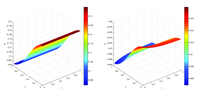
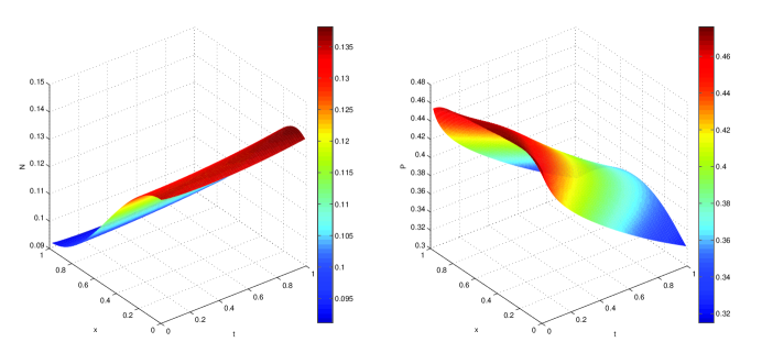
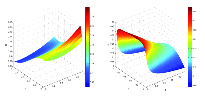
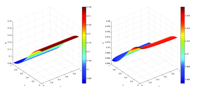
In Figs 1-5, we use the fractional centered difference scheme to show different numerical solutions preserving the positivity and boundedness with the mesh $h=\tau=0.01$. We observe that the orders $\alpha$ and $\beta$ affect the shape of the solutions obviously. Fig. 1 shows the solutions of classical predator-prey reaction-diffusion model with $\alpha=1$ and $\beta=2$. When $\alpha$ tends to 1 and $\beta$ to 2, the numerical solutions of the fractional predator-prey reaction-diffusion equations are also convergent to the solutions of the classical ones.

Figure 1. Numerical solution for the case $\alpha=1$ and $\beta=2$

Figure 2. Numerical solution for the case $\alpha=1$ and $\beta=1.9$

Figure 3. Numerical solution for the case $\alpha=1$ and $\beta=1.5$

Figure 4. Numerical solution for the case $\alpha=0.5$ and $\beta=2$

Figure 5. Numerical solution for the case $\alpha=0.5$ and $\beta=1.5$

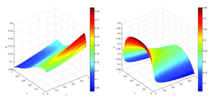
To get the convergent order in time and space, we consider the nonhomogeneous equations:

$$\begin{array}[]{llll}\displaystyle\frac{\partial^{\alpha}N}{\partial t^{\alpha}}&=&D_{1}\displaystyle\frac{\partial^{\beta}N}{\partial|x|^{\beta}}+N\left(1-N-\frac{\varrho P}{P+N}\right)+f(x,t),\\ \\ \displaystyle\frac{\partial^{\alpha}P}{\partial t^{\alpha}}&=&D_{2}\displaystyle\frac{\partial^{\beta}P}{\partial|x|^{\beta}}+\sigma P\left(-\frac{\gamma+\kappa\delta P}{1+\kappa P}+\frac{N}{P+N}\right)+g(x,t).\end{array}$$

Suppose that the exact solution is

$$N(x,t)=P(x,t)=(t+1)^{2}x^{2}(1-x)^{2},$$

and the nonhomogeneous terms are

$$f(x,t)= 2(-1+x)^{2}x^{2}(\frac{t^{1-\alpha}}{\Gamma(2-\alpha)}+\frac{t^{2-\alpha}}{\Gamma(3-\alpha)})$$

$$+\frac{D_{1}(1+t)^{2}}{\Gamma(5-\beta)}x^{-\beta}(\frac{(-1+x)^{2}x^{\beta}}{(1-x)^{\beta}}(12x^{2}-6x\beta+(-1+\beta)\beta)$$

$$+x^{2}(12(-1+x)^{2}+(-7+6x)\beta+\beta^{2}))\sec(\frac{\pi\beta}{2})$$

$$-(t+1)^{2}x^{2}(1-x)^{2}(1-(t+1)^{2}x^{2}(1-x)^{2}-\varrho/2),$$

$$g(x,t)= 2(-1+x)^{2}x^{2}(\frac{t^{1-\alpha}}{\Gamma(2-\alpha)}+\frac{t^{2-\alpha}}{\Gamma(3-\alpha)})$$

$$+\frac{D_{2}(1+t)^{2}}{\Gamma(5-\beta)}x^{-\beta}(\frac{(-1+x)^{2}x^{\beta}}{(1-x)^{\beta}}(12x^{2}-6x\beta+(-1+\beta)\beta)$$

$$+x^{2}(12(-1+x)^{2}+(-7+6x)\beta+\beta^{2}))\sec(\frac{\pi\beta}{2})$$

$$-\sigma(t+1)^{2}x^{2}(1-x)^{2}(-\frac{\gamma+\kappa\delta(t+1)^{2}x^{2}(1-x)^{2}}{1+\kappa(t+1)^{2}x^{2}(1-x)^{2}}+1/2).$$

Table 1 shows that the method has first-order accuracy for the time discretizations when $\alpha=0.5$ and $\beta=1.5$. In the computations of the example, we take the spacial steplength $h=0.005$, which is small enough so that the error in space direction can be neglected for getting convergent rate. Table 2-4 show that the fractional centered difference scheme has second-order accuracy for different cases, and Table 5 and 6 show that the WSGD scheme also has second-order accuracy. In these cases, we consider the errors with temporal steplength $\tau=0.0001$, which is small enough so that the error in time direction can be neglected for getting the convergent rate.

Table 1. The numerical errors and convergent orders for the time discretization with $\alpha=0.5$ and $\beta=1.5$ (the space derivative is discretized by the fractional centered difference scheme).

$\tau(h=0.005)$	$e_{N}(h,\tau)$	rate	$e_{P}(h,\tau)$	rate
$0.1$	$0.003082147971456$		$0.003879257478438$
$0.05$	$0.001660319792980$	$0.89247$	$0.002045107336033$	$0.92360$
$0.025$	$8.702233156421824e-04$	$0.93200$	$0.001057717860272$	$0.95122$
$0.0125$	$4.486628201542942e-04$	$0.95575$	$5.405498347547111e-04$	$0.96846$

Table 2. The numerical errors and convergent orders of the fractional centered difference scheme with $\alpha=0.5$ and $\beta=1.5.$

$h(\tau=0.0001)$	$e_{N}(h,\tau)$	order	$e_{P}(h,\tau)$	order
$0.1$	$0.002448567676975$		$0.012304879445640$
$0.05$	$4.333240674121927e-04$	$2.4984$	$0.001897961774831$	$2.6967$
$0.025$	$4.078185842617405e-05$	$3.4094$	$1.770846542422655e-04$	$3.4219$
$0.0125$	$7.936093047861137e-06$	$2.3614$	$2.735531025410687e-05$	$2.6945$

Table 3. The numerical errors and convergent orders of the fractional centered difference scheme with $\alpha=0.5$ and $\beta=1.1.$

$h(\tau=0.0001)$	$e_{N}(h,\tau)$	order	$e_{P}(h,\tau)$	order
$0.1$	$0.001017521017230$		$0.004047202939302$
$0.05$	$1.098732300429083e-04$	$3.2174$	$4.503780973269950e-04$	$3.1677$
$0.025$	$1.518595837027292e-05$	$2.8437$	$6.202433574753474e-05$	$2.8825$

Table 4. The numerical errors and convergent orders of the fractional centered difference scheme with $\alpha=0.5$ and $\beta=1.9.$

$h(\tau=0.0001)$	$e_{N}(h,\tau)$	order	$e_{P}(h,\tau)$	order
$0.1$	$0.007646089314486$		$0.044021358056344$
$0.05$	$0.002075492029463$	$1.8813$	$0.010198249263744$	$2.1099$
$0.025$	$4.102572803958426e-04$	$2.3389$	$0.001878050620810$	$2.4410$
$0.0125$	$6.289181719891512e-05$	$2.7056$	$2.648747633180820e-04$	$2.8259$

Table 5. The numerical errors and convergent orders of the WSGD scheme with $\alpha=0.5$ and $\beta=1.1.$

$h(\tau=0.0001)$	$e_{N}(h,\tau)$	order	$e_{P}(h,\tau)$	order
$0.1$	$8.143435340095817e-04$		$0.003968570949633$
$0.05$	$4.211307291067442e-04$	$0.95137$	$0.001501172252600$	$1.4025$
$0.025$	$1.523958731684217e-04$	$1.4664$	$6.213886912121139e-04$	$1.2725$
$0.0125$	$3.564037214530500e-05$	$2.0962$	$2.003495389639826e-04$	$1.6330$

Table 6. The numerical errors and convergent orders of the WSGD scheme with $\alpha=0.5$ and $\beta=1.9$ .

$h(\tau=0.0001)$	$e_{N}(h,\tau)$	order	$e_{P}(h,\tau)$	order
$0.1$	$0.017922317172642$		$0.091921901959502$
$0.05$	$0.005756704773643$	$1.6384$	$0.025183003437663$	$1.8680$
$0.025$	$0.001233852922224$	$2.222$	$0.005115931266937$	$2.2994$
$0.0125$	$0.000178819437800$	$2.7866$	$0.000661363526132$	$2.9515$

6. Conclusion

More than three decades ago, the classical diffusion is introduced into the predator-prey model, which leads to the predator-prey reaction-diffusion model. With the deep research on the anomalous diffusion, it is noticed that the anomalous diffusion is ubiquitous. It seems nature to introduce the anomalous diffusion to the predator-prey model, then we get the space-time fractional predator-prey reaction-diffusion model. This paper proves that the analytical solutions of the model are positive and bounded; and we provide the semi-implicit numerical schemes with the first-order accuracy in time and second-order accuracy in space. The proposed schemes are proven to be stable and preserve the positivity and boundedness. And the theoretical results are confirmed by numerical experiments.

References

- [1] F. Brauer and C. Castillo-Chavez, \doititle“Mathematical Models in Population Biology and Epidemiology”, Springer-Verlag, 2000.
- [2] E. D. Conway and J. A. Smoller, Diffusion and the predator-prey interaction, SIAM J. Appl. Math., 33 (1977), 673-686.
- [3] M. Cavani and M. Farkas, Bifurcation in a predator-prey model with memory and diffusion II: Turing bifurcation, Acta Math. Hungar., 63 (1994), 375-393.
- [4] S. Aly, I. Kim and D. Sheen, Turing instability for a ratio-dependent predator-prey model with diffusion, Appl. Math. Comp., 217 (2011), 7265-7281.
- [5] F. Bartumeus, D. Alonso, and J. Catalan, Self organized spatial structures in a ratio dependent predator-prey model, Phys. A, 295 (2001), 53-57.
- [6] P. Y. H. Pang and M. X. Wang, Qualitative analysis of a ratio-dependent predator prey system with diffusion, Proc. R. Soc. Edinb., 133(A) (2003), 919-942.
- [7] M. Wang, Stationary patterns for a prey predator model with prey-dependent and ratio-dependent functional responses and diffusion, Physica D, 196 (2004), 172-192.
- [8] A. Yun, D. Jeong, and J. Kim, An Efficient and Accurate Numerical Scheme for Turing Instability on a Predator-Prey Model, Int. J. Bifur. Chaos, 22(6) (2012), 1250139.
- [9] R. Metzler and J. Klafter, The random walk’s guide to anomalous diffusion: a fractional dynamics approach, Phys. Rep., 339(1) (2000), 1-77.
- [10] Y. Y. Yu, W. H. Deng, and Y. J. Wu, Positivity and boundedness preserving schemes for the fractional reaction-diffusion equation, Sci. China Math., 56(10) (2013), 2161-2178.
- [11] M. M. Meerschaert, H.P. Scheffler, and C. Tadjeran, Finite difference methods for two-dimensional fractional dispersion equation, J. Comput. Phys., 211 (2006), 249-261.
- [12] Q. Yang, F. Liu, and I. Turner, Numerical methods for fractional partial differential equations with Riesz space fractional derivatives, Appl. Math. Model., 34(1) (2010), 200-218.
- [13] C. Chen, F. Liu, I. Turner, and V. Anh, A Fourier method for the fractional diffusion equation describing sub-diffusion, J. Comput. Phys., 227 (2007), 886-897.
- [14] M. R. Cui, Compact finite difference method for the fractional diffusion equation, J. Comput. Phys., 228 (2009), 7792-7804.
- [15] G. Gao and Z. Sun, A compact difference scheme for the fractional sub-diffusion equations, J. Comput. Phys., 230 (2011), 586-595.
- [16] Y. Lin and C. Xu, Finite difference/spectral approximations for the time-fractional diffusion equation, J. Comput. Phys., 225 (2007), 1533-1552.
- [17] S. B. Yuste and L. Acedo, An explicit finite difference method and a new Von-Neumann Type stability analysis for fractional diffusion equations, SIAM J. Numer. Anal. 42 (2005), 1862-1874.
- [18] W. H. Deng, Numerical algorithm for the time fractional Fokker-Planck equation, J. Comput. Phys., 227 (2007), 1510-1522.
- [19] M. D. Ortigueira, Riesz potential operators and inverses via fractianal centred derivatives, International J. Math. Math. Sci., 2006 (2006), 48391.
- [20] C. Celik and M. Duman, Crank-Nicolson method for the fractional diffusion equation with the Riesz fractional derivative, J. Comput. Phys., 231 (2012), 1743-1750.
- [21] D. Wang, A. Xiao, and W. Yang, Crank-Nicolson difference scheme for the coupled nonlinear Schrödinger equations with the Riesz space fractional derivative, J. Comput. Phys., 242 (2013), 670-681.
- [22] W. Y. Tian, H. Zhou, and W. H. Deng, A class of second order difference approximation for solving space fractional diffusion equations, \arXiv1201.5949 [math.NA].
- [23] H. Zhou, W. Y. Tian, and W. H. Deng, Quasi-compact finite difference schemes for space fractional diffusion equations, J. Sci. Comput., 56(1) (2013), 45-66.