TIGER: A data analysis pipeline for testing the strong-field dynamics of general relativity with gravitational wave signals from coalescing compact binaries
Abstract
The direct detection of gravitational waves with upcoming second-generation gravitational wave observatories such as Advanced LIGO and Advanced Virgo will allow us to probe the genuinely strong-field dynamics of general relativity (GR) for the first time. We have developed a data analysis pipeline called TIGER (Test Infrastructure for GEneral Relativity), which uses signals from compact binary coalescences to perform a model-independent test of GR. In this paper we focus on signals from coalescing binary neutron stars, for which sufficiently accurate waveform models are already available which can be generated fast enough on a computer that they can be used in Bayesian inference. By performing numerical experiments in stationary, Gaussian noise, we show that for such systems, TIGER is robust against a number of unmodeled fundamental, astrophysical, and instrumental effects, such as differences between waveform approximants, a limited number of post-Newtonian phase contributions being known, the effects of neutron star tidal deformability on the orbital motion, neutron star spins, and instrumental calibration errors.
pacs:
04.80.Nn, 02.70.Uu, 02.70.RrI Introduction and overview
General relativity (GR) is a highly non-linear, dynamical theory of gravity. Yet, until the 1970s, almost all of its tests were based on the behavior of test particles in a static gravitational field MTW , such as the perihelion precession of Mercury, the deflection of starlight by the Sun, and Shapiro time delay. The parameterized post-Newtonian (PPN) formalism (for an overview, see Will2006 ) was developed as a systematic framework for these and other tests; even so, the interpretation of most of the available data did not require much more than an expansion of the Schwarzschild metric in , with the mass and the distance, up to the first few non-trivial orders. Although excellent agreement with theory was obtained, the tests that were actually performed amounted to little more than probing the effect on the motion of test masses of low-order general relativistic corrections to the Newtonian gravitational field.
The situation improved with the discovery of the Hulse-Taylor binary neutron star in 1974 ht75 . One of the components could be observed electromagnetically as a pulsar, and this way it was inferred that the binary loses energy and angular momentum through gravitational wave (GW) emission as predicted by GR, at least at the level of the quadrupole formula Weisberg2010 . Subsequently, more relativistic binaries were discovered, allowing for impressive new tests of GR in a parameterized post-Keplerian (PPK) framework Freire2012 . However, if one is interested in further probing the dissipative dynamics of binaries, and especially the dynamics of spacetime itself, what matters is the orbital compactness (with the total mass and the separation), as well as the orbital velocity . Even the newly discovered neutron star-white dwarf system Antoniadis2013 only has , and . For comparison, the surface gravity of the Sun is , and the orbital velocity of Mercury is .
By contrast, binaries consisting of neutron stars and/or black holes on the verge of merger will have and , with copious gravitational wave emission. Being able to observe the orbital motion of such systems would give us access to the genuinely strong-field, relativistic regime of gravity. Most importantly, we would like to probe the dynamical self-interaction of spacetime itself, such as the scattering of quadrupolar waves off the Schwarzschild curvature generated by the binary as a whole Blanchet1994 ; Blanchet1995 . The only way to gain empirical access to such phenomena is through direct gravitational wave detection.
A network of second-generation gravitational wave detectors is currently under construction. The Advanced LIGO aLIGO and Advanced Virgo AdV GW observatories are expected to start taking data in 2015, with gradual upgrades in the following years. The smaller GEO-HF in Germany is already active GEO . KAGRA KAGRA in Japan and possibly LIGO-India IndIGO will come online a few years later. These detectors may find tens of GW signals per year from coalescing compact binaries composed of two neutron stars (BNS), a neutron star and a black hole (NSBH), or two black holes (BBH). The predicted detection rates for the Advanced LIGO-Virgo network are in the range depending on the astrophysical event rate, the instruments’ duty cycle, and the sensitivity evolution of the detectors rates ; commissioning ; see also Chen2012 for detection rate predictions assuming that short, hard gamma ray bursts are caused by coalescing binaries.
There is a considerable body of literature on the constraints that can be put on various specific alternative theories of gravity with ground-based and space-based GW detectors, and pulsar timing arrays; see Gair2012 ; Yunes2013 and references therein. What we will be interested in here are model-independent tests of GR itself. A first step in that direction was taken by Arun et al. Arun2006a ; Arun2006b ; Mishra2010 in the context of compact binary inspiral. Their method exploits the fact that, at least for binaries where neither component has spin, all coefficients in the post-Newtonian (PN) expansion of the inspiral phase (see below for their definition) only depend on the component masses , . Hence only two of them are independent, and a comparison of any three of them allows for a test of GR. Such a method would be extremely general, in that one does not have to look for any specific way in which GR might be violated; instead, very generic deviations can be searched for. A similar idea was pursued in the context of ringdown by Gossan et al. Gossan2012 : if the No Hair Theorem applies to Nature, then the frequencies and damping times of the various ringdown modes again only depend on two quantities, in this case the mass and spin of the final black hole.
The original ideas of Arun2006a ; Arun2006b ; Mishra2010 have the drawback that they rely on parameter estimation, which makes it difficult to combine information from multiple sources. An alternative way of testing GR is Bayesian model selection. Here one compares two hypotheses, one corresponding to the GW waveform model predicted by GR, and the other to a model which has parameterized deformations of the GR waveform, characterized by additional parameters . This was the approach taken by Del Pozzo et al. DelPozzo2011 in the context of inspiral (where a single additional parameter was introduced, related to the graviton mass), and again by Gossan et al. for ringdown (where multiple extra free parameters were considered) Gossan2012 . Yunes and collaborators Yunes2009 ; Cornish2011 ; Chatziioannou2012 proposed a parameterization of non-GR waveforms guided by the ways in which a variety of alternative theories of gravity modify the GR waveform, leading to the “parameterized post-Einsteinian” (PPE) framework. For the relationship between the PPN, PPK, and PPE formalisms, see Sampson2013 .
In the abovementioned Bayesian studies, a comparison was made between a waveform model in which all the extra parameters were allowed to vary, and a waveform model where all of them took their GR values (which for the present discussion we can take to mean for ). As noted by Li et al. Li2012a , this corresponds to asking the question “Do all of the differ from zero at the same time?” Let us denote the associated hypothesis by , which is to be compared with the GR hypothesis . A more general (and hence more interesting) question is: “Do one or more of the differ from zero?” Denote the corresponding hypothesis by . As shown in Li2012a , although there is no single waveform model associated with , testing the latter amounts to testing disjoint sub-hypotheses corresponding to all subsets of the full set of “testing parameters” . A given is tested by a waveform model in which are free, but all the other are fixed to zero. The Bayes factors against GR for all of these sub-hypotheses can be combined into a single odds ratio which compares with .
In the present paper, we will consider deformations in the inspiral phase of the waveform, which in the stationary phase approximation Thorne1987 ; Sathyaprakash1991 takes the form
| (1) |
where and are, respectively, the time and phase at coalescence, and in GR, the coefficients , are specific, known functions of the component masses , and spins , . Parameterized deformations of the phase can be introduced by writing , where is the expression for as a function of component masses , and spins , that GR predicts.111One could also introduce parameterized deformations of the amplitude, but studies have shown that for low-mass systems, second-generation detectors will not be very sensitive to sub-leading effects in the amplitude VanDenBroeck2007a ; VanDenBroeck2007b ; OShaughnessy2013 .
Given a catalog of sources detected with the dedicated search pipelines Beauville2005 ; Brown2005 ; Babak2006 ; Cokelaer2007a ; Cokelaer2007b ; VanDenBroeck2009 ; Brown2012 ; Babak2013 ; Brown2013 , assuming equal prior odds for all the sub-hypotheses and taking the data streams for the individual detections to be independent, the odds ratio for against yields Li2012a ; Li2012b ; VanDenBroeck2013
with and the evidences for and , respectively; denotes any background information we may hold, and is the ratio of prior odds for against .
If GR happens to be valid then one would expect , or . However, the noise in the detectors can mimic violations of GR, so that one can have even if GR is in fact the correct theory of gravity. Moreover, there will be some effect of numerical inaccuracy in the calculation of the log odds ratio. To make sure that we will not erroneously declare a GR violation, the measured log odds ratio will be compared with a background distribution. The latter is constructed by taking a large number of simulated GR signals, all having different masses, sky locations, orientations, and distances picked from astrophysically motivated distributions (see Sec. II below), and injecting them into stretches of data surrounding the ones the detections are in, to have similar noise realizations. Here one can adopt the treatment of “on-source” and “off-source” data as in searches for gravitational wave events associated with gamma ray bursts; see S6GRB and references therein. These injections can be combined randomly into “catalogs”, each containing however many sources were observed in reality. For every catalog of background injections one can calculate , arriving at an estimate for the distribution of the log odds ratio for the case where GR is correct. Given such a distribution and picking a maximum tolerable false alarm probability, a threshold can be computed for the measured log odds ratio to overcome.
For details of the above definitions and derivations, we refer to Li2012a ; Li2012b ; VanDenBroeck2013 . As explained in those references and further elucidated in this paper, the approach of Li et al. has several attractive features:
-
(i)
One can use an arbitrarily large number of “testing parameters” without having to worry about a model being insufficiently parsimonious in cases where the true number of non-GR parameters is small, due to the availability of sub-hypotheses corresponding to different numbers of free parameters.
-
(ii)
Information from multiple sources can trivially be combined, leading to a stronger test of GR.
-
(iii)
It is well-suited to a regime where most sources have a small signal-to-noise ratio, again because of the use of multiple non-GR sub-hypotheses.
-
(iv)
It will allow us to find a wide range of deviations from GR, even ones that are well outside the particular parameterized waveform family used.
-
(v)
The method is not tied to any given waveform model, or even any particular part of the coalescence process.
Given these advantages, it is natural to take the above scheme as a basis for computer code to test GR using actual detector data. Such a data analysis pipeline is now in place within the LIGO Algorithm Library LAL . It is called TIGER, for “Test Infrastructure for GEneral Relativity”.
Before we can be sure of the usefulness of TIGER in a realistic data analysis setting, we must check its robustness against any unknown fundamental, astrophysical, and instrumental effects. We focus on BNS, since for this case, waveform models that accurately capture the relevant physics and can be generated sufficiently fast on a computer have been available for some time now Buonanno2009 . In practice, BNS systems could be selected for by looking at the chirp mass , a parameter which tends to be very well determined in gravitational wave parameter estimation, with uncertainties of a few percent.222Here we are referring to both statistical and systematic errors; see S6PE for examples. In Dominik et al. Dominik2012 , results from a large number of formation models for compact binaries are given. They find the minimum chirp mass for NSBH to be , and for BBH. Thus, selecting only detections for which e.g. at 95% confidence should remove all NSBH and BBH events. Of course, it is entirely possible that some genuine BNS detections will be removed in this way (in fact, this is what the BNS results of Dominik2012 suggest), but the procedure is a conservative one. We note that of necessity, the selection will have to be done based on parameter estimation with GR waveforms. If GR is incorrect, then there could be a large bias in the measurement of (among other parameters) Yunes2009 ; DelPozzo2011 ; Li2012a ; Vitale2014 , in which case even a BBH system could be mis-classified as a BNS system. However, in that case we expect TIGER to a fortiori indicate a violation of GR.
Focusing on BNS, the following issues need to be addressed:
-
(i)
Even for binary neutron star coalescence, there are small differences between the various waveform approximants that are available. Since TIGER is specifically designed to find anomalies in the signals, we must make sure that these discrepancies, however minor, are not mistaken for violations of GR.
-
(ii)
Post-Newtonian waveforms are only available up to 3.5PN in phase. What might be the effect of unknown PN contributions?
-
(iii)
In the final stages of inspiral, neutron stars get deformed because of each other’s tidal fields. This has an effect on the orbital motion, which gets imprinted onto the GW signal waveform. The size of these tidal effects is set by the neutron star equation of state, about which currently not much is known. Can we avoid mistaking unknown tidal effects for a violation of GR?
-
(iv)
The dimensionless spins of neutron stars in binaries are generally expected to be quite small, but the resulting spin-orbit and spin-spin effects will nevertheless need to be taken into account.
-
(v)
The calibration of the instruments will be imperfect, leading to frequency dependent uncertainties in the interpretation of amplitudes and phases. What will their impact be?
In order to see how these effects can be brought under control, we perform numerical experiments in simulated stationary, Gaussian noise following the predicted noise curves of Advanced LIGO and Advanced Virgo at their final design sensitivities aLIGO ; AdV . Note that in reality, the noise will be neither Gaussian nor stationary due to “glitches”. As explained above, TIGER involves the calculation of a background distribution in which these additional unknowns will be included automatically, possibly resulting in a widening of the background. However, here we focus on the points above; further instrumental issues will be dealt with in a forthcoming study.
This paper is structured as follows. In Sec. II, we explain the setup of the simulations, and how we will compare results arising from different assumptions. The main results are presented in Sec. III, where we show how TIGER can be made robust against differences between waveform approximants, limited availability of post-Newtonian phase contributions, unknown neutron star tidal deformability, instrumental calibration errors, and the effects of neutron star spins. Conclusions and future directions are discussed in Sec. IV.
Unless stated otherwise, we will use units such that .
II Setup of the simulations and comparison of results
The results in this paper pertain to simulations of BNS signals in stationary, Gaussian noise following the design sensitivity of Advanced LIGO and Advanced Virgo aLIGO ; AdV . Component masses were in the range ,333This means that in the simulations, we don’t quite use the cut proposed above, but our key results are unlikely to be affected by this choice. sky positions and orientations were chosen from uniform distributions on the sphere, and sources were placed uniformly in co-moving volume with luminosity distance Mpc. Depending on the type of robustness test, the signal waveform was taken to be TaylorF2 with zero or (anti-)aligned spins, or TaylorT4 with precessing spins; the recovery was done with TaylorF2 waveforms, again with either zero or (anti-)aligned spins. Only sources with optimal network SNR above 8 were taken into account Cutler1993 . Occasionally it would happen that a source survived the SNR cut without being found by the GR waveform model, meaning , with the log Bayes factor for the hypothesis of a GR signal being present against the noise-only hypothesis. Such sources were discarded by imposing , motivated by the fact that the main contribution to is , with the GR waveform, and is the usual noise-weighted inner product Maggiore :
| (3) |
where a tilde denotes the Fourier transform, and is the one-sided noise power spectral density. To compute the evidences and we used the nested sampling method as implemented by Veitch and Vecchio Veitch2008a ; Veitch2008b ; Veitch2010 , with 1000 “live points” and 100 “MCMC points”, which leads to an uncertainty in log Bayes factors against noise Veitch2010 .
In what follows, we will want to compare different background distributions: with or without calibration errors, with or without tidal effects in the injections, and so on. A convenient way of quantifying the difference between distributions is by means of the Kolmogorov-Smirnov statistic Kolmogorov1933 ; Smirnov1948 . Consider backgrounds and for different injection sets , (or in the case of calibration errors, different simulated data sets containing injections). Construct the cumulative distributions of log odds ratio and call these and , respectively; here and are the numbers of log odds ratio values that are available in each of the two cases. Then the Kolmogorov-Smirnov (KS) statistic is just the largest distance between the cumulative distributions:
| (4) |
Note that by construction, this is a number between 0 and 1. If , then the difference between the background distributions can be considered small.
III Robustness of TIGER against unknown fundamental, astrophysical, and instrumental effects
We now show how the TIGER pipeline can be made robust against effects of a fundamental, astrophysical, or instrumental nature which can not easily be accounted for in our waveform models. In turn, we study the impact of neutron star tidal deformability, differences between waveform approximants, unknown contributions to the phase at high PN order, instrumental calibration errors, the effect on the background of the number of coefficients used, and precessing neutron star spins. We expressly gauge the importance of each of these issues separately, in order to clearly demonstrate how each of them can be brought under control, before finally considering the situation where all of them are jointly present.
III.1 Neutron star tidal deformability
As two neutron stars spiral towards each other, each will get deformed due to the tidal field of the other. These deformations have an influence on the orbital motion which gets imprinted onto the emitted gravitational wave signal. The size of the effect is set by the tidal deformability , which relates the Newtonian tidal tensor of one star to the induced quadrupole moment of the other: . One has , with the second Love number and the neutron star radius. As the notation suggests, the tidal deformability depends on mass in a way that is determined by the neutron star equation of state (EOS). In the presence of tidal effects, the waveform phase takes the form , where is the usual point particle contribution, and to 1PN beyond leading order for tidal contributions one has444Damour, Nagar, and Villain have computed tidal contributions to 2.5PN Damour2012 , but these were not yet available when this work was started. Hinderer2009
| (5) |
The sum is over the components of the binary, and , for . Note that although these contributions occur at 5PN and 6PN in the phase, they come with a prefactor that is potentially quite large: Lattimer2013 , so that the effect can be noticeable even with second-generation detectors. Indeed, in DelPozzo2013 it was shown that, if one assumes GR to be correct, the EOS can be significantly constrained by combining information from BNS observations. This in turn means that tidal effects could be mistaken for GR violations.
Since little is known about the EOS – in fact, currently the tidal deformability is uncertain by an order of magnitude – we have no way of including an accurate description of it in our waveform models. However, because of the high PN order at which these effects occur, they will only be important at very high frequencies. Indeed, as shown by Hinderer et al. Hinderer2009 (see also the recent work by Read et al. Read2013 ), with second-generation detectors they only become noticeable for Hz. For this reason we terminate our template waveforms at Hz (which in terms of characteristic velocity and compactness corresponds to and , respectively). As it turns out, this leads to a loss in SNR of less than a percent, and in any case TIGER mostly probes the lower PN orders, corresponding to lower frequencies. However, here too we want to explicitly check that this suffices to make TIGER impervious to the unknown effect.
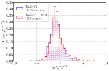
In Fig. 1, we compare the background for TaylorF2 injections without tidal effects, with the background obtained from injections with a very hard EOS (corresponding to large deformability), namely the one labeled MS1 in Hinderer2009 . The injected waveforms are taken to terminate at LSO while the recovery waveforms (also TaylorF2) are cut off at 400 Hz in both cases.
Consider the background distribution for “point particle” (PP) injections (no tidal effects), , and the distribution of log odds ratio for MS1 injections , . Using the cumulative distributions of log odds in the two cases, one can construct the Kolmogorov-Smirnov statistic as in Eq. (4). For the injection sets , used in Fig. 1, we find , indicating that the two background distributions are very close to each other. We conclude that the 400 Hz cut-off renders tidal effects invisible without affecting TIGER’s ability to look for GR violations.
Below we will continue to implement a 400 Hz cut-off in the recovery waveforms.
III.2 Differences between waveform approximants
For all the post-Newtonian waveform approximants, the phase and instantaneous velocity (or equivalently ) are computed from the conserved energy per unit mass and the gravitational wave flux through Kepler’s law and the flux-energy balance equation:
| (6) | |||||
| (7) |
where the prime denotes derivation with respect to . The solutions take the general form
| (8) | |||||
| (9) |
where and are integration constants, and is an arbitrary reference velocity. Now, since and are known as series expansions in up to a finite order, there are multiple ways of treating the above equations. In the case of the so-called TaylorT1 approximant, is kept as a ratio of polynomials, and Eqns. (6) and (7) are solved numerically. In the case of TaylorT4, what one does instead is to expand the ratio and truncate the result at the consistent PN order, after which Eqns. (6), (7) are again solved numerically. TaylorT2 is obtained by expanding and consistently truncating , and integrating Eqns. (8) and (9) to obtain a pair of transcendental equations for and as functions of , which are then solved numerically. For TaylorT3 one also expands and truncates , and integrates Eqns. (8) and (9) to obtain expressions for and . The latter is inverted to , and a representation of is computed. Finally, the frequency domain TaylorF2 approximant is obtained through the stationary phase approximation, by utilizing a saddle point in the calculation of the Fourier transform of the time domain waveform. For more details on all these approximants, see Buonanno2009 and references therein.
A qualitatively different way of obtaining waveform models is the effective-one-body (EOB) method. Here a mapping is established between the motion of the two component masses and the motion of a single particle in an effective metric, which is captured by a set of Hamiltonian equations for the angular and radial motion. These are solved numerically. The advantage of this method is that the resulting waveforms are reliable up to later times compared to the PN ones (well into the plunge preceding merger), which also means that they lend themselves particularly well to being further “tuned” using input from numerical simulations after being completed with a ringdown waveform. Here too we point to Buonanno2009 and references therein for further information.
The authors of Buonanno2009 calculated the effectualness and faithfulness of post-Newtonian waveforms with respect to each other, as well as with an EOB waveform model tuned using numerical simulations, and this for a variety of component masses. The effectualness is a measure of how effective a waveform model will be when used as a template to detect a “signal” waveform ; for given intrinsic and extrinsic signal parameters , it is defined as , where , and is again the usual noise-weighted inner product Maggiore . In the case of faithfulness, the intrinsic parameters of “signal” and “template” are taken to be the same, and the maximization is only over the template’s time and phase at coalescence: . In the expected mass range of NSBH and BBH, there can be significant differences between the PN approximants amongst themselves, and with EOB waveforms. However, in the BNS mass range, at least in the case of zero spins, both the effectualness and faithfulness for any pair of PN waveforms and for any PN approximant with the EOB model tend to be above 0.99.555An exception is the so-called TaylorEt waveform, which is considered pathological for this reason. For example, in the case of Advanced LIGO and for , the faithfulness of TaylorF2 against TaylorT4 is 0.999, and for TaylorF2 against EOB it is 0.996.
The strong agreement between the various waveform approximants in the BNS mass range suggests that, at least for such systems, it is safe to adopt TaylorF2, the computationally least expensive waveform model, for the trial waveforms used in TIGER. However, since the pipeline is specifically meant to find small anomalies in the signals, we need to make sure that even small differences between waveform approximants are not mistaken for violations of GR.
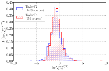
In Fig. 2, we compare single-source background distributions for the case where the GR signals are TaylorT4 waveforms and the case where they are TaylorF2 waveforms; but, in both cases, the analysis of the data is done with TaylorF2. Once again the difference between the two distributions can be quantified by using the KS statistic, which in this case comes out to be .
Due to computational cost, we decided not to repeat the calculation with TaylorT1, TaylorT2, TaylorT3, or EOB injections. However, the results of Fig. 2, together with the waveform comparisons of Buonanno2009 , are sufficient to conclude that TIGER will not mistake differences in waveform models for violations of GR.
III.3 Effect of post-Newtonian order
In Buonanno2009 , waveform approximants were considered up to 3.5PN in phase, which is the highest post-Newtonian order currently available. To this order, post-Newtonian waveforms and EOB-based inspiral-merger-ringdown waveforms that were tuned using numerical relativity simulations agree extremely well in the BNS mass regime. However, taking numerical relativity results to be the benchmark for how realistic a waveform model is, we note that large-scale numerical simulations of spacetimes containing coalescing binaries still only give information about the last few tens of cycles Ajith2012 , whereas a typical BNS waveform is thousands of cycles long. Thus, it could be that adequate modeling of the signals by post-Newtonian waveforms will require going to still higher PN order in the phase.666It is also possible that the contrary is true, since it is not known whether the post-Newtonian expansion converges Simone1997 .
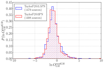
In Fig. 3, we probe the effect on the background of differences in post-Newtonian order between signal and recovery waveforms, for TaylorF2. In one case, both are taken to 3.5PN order, while in the other case the signal is 3.5PN whereas the recovery waveform only goes to 3PN. We see that the distributions barely differ; the KS statistic is . Needless to say, this does not prove that missing post-Newtonian orders beyond 3.5PN will be unproblematic, but it does lend further confidence to the soundness of our approach. Note also that one can expect high PN contributions to manifest themselves at high frequencies, and our recovery waveforms are cut off at 400 Hz.
III.4 Instrumental calibration errors
Imperfect calibration of the instruments can cause one to draw incorrect conclusions about detected signals. Calibration errors affect the instruments’ transfer functions , which relate external length changes in the interferometer arms to the detector outputs :
| (10) |
is a complex function, which can be written in polar form as
| (11) |
where and are frequency dependent calibration errors in amplitude and phase, respectively, and is the transfer function in the absence of errors. The frequency domain data stream is given by
| (12) |
where is the interferometer arm length in the absence of disturbances. Calibration errors affect both the data stream and the power spectral density of the noise , but not the model waveforms corresponding to the hypotheses and , which is how parameter estimation and model selection get affected by them.
In Vitale2012 , the calibration errors were modeled based on the errors measured in the initial LIGO and Virgo instruments, and their effect on Bayesian parameter estimation and model selection for advanced detectors was assessed. It was found that even with amplitude errors of and phase errors degrees in each instrument, for 90% of sources the systematics induced will be less than 20% of the statistical uncertainties in parameter estimation. Similarly, model selection is not much affected by calibration errors.
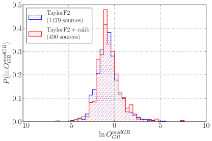
Fig. 4 shows the effect of calibration errors, modeled exactly as in Vitale2012 , on the log odds ratio background distribution. As expected, the effect is minor (with ), and calibration errors will not affect the performance of TIGER.
III.5 Number of testing parameters
TIGER allows one to circumvent the usual problem in Bayesian analysis when the number of extra parameters in the model is too large: The total number of testing parameters, , can in principle be arbitrarily large without risk of being penalized by the high dimensionality of the parameter space should the number of extra parameters in the signal be smaller than . One aspect of this was already illustrated in Li2012a , where it was shown that if the GR violation is limited to e.g. the 1.5PN phase coefficient, hypotheses with too many free parameters tend to be disfavored even if they include . However, what also needs to be checked explicitly is how sensitive the background is to the number of testing parameters: Should it be the case that it widens dramatically as is increased because features in the noise can more easily be accommodated by waveforms with more free parameters, then the advantage disappears. In Fig. 5, we compare backgrounds for and , and the difference turns out to be small; in terms of a KS statistic, .
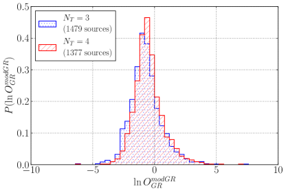
Together with the results of Li2012a , this indicates that one should use as many testing parameters as possible. However, in practice there will be computational constraints due to the exponential growth of the number of sub-hypotheses with the total number of testing parameters; indeed, for testing parameters, sub-hypotheses need to be compared with . The results of Li2012a ; Li2012b suggest that in the case of BNS, the sensitivity of TIGER to GR violations occurring above 2PN order in phase will be limited. In the examples below, we use three testing parameters, .
III.6 Neutron star spins
The observed pulsar spin periods and assumptions about neutron star spindown rates lead to periods at birth in the range 10–140 ms Lorimer2008 , corresponding to dimensionless spins , and the fastest known pulsar in a BNS has a spin . Thus, neutron star spins in BNS systems are generally expected to be small. Nevertheless, we need to quantify their effect on the background distribution and hence the detectability of GR violations.
In the phase, spin-orbit effects first appear at 1.5PN order, and spin-spin effects at 2PN. The amplitude is also affected, primarily because of spin-induced precession of the orbital plane, which causes the inclination angle to change so that sometimes a system might be close to being face-on whereas at other times it will be closer to being edge-on, causing amplitude modulation.
To describe the orbital motion with inclusion of spins, one again uses the Kepler and flux-energy balance equations, Eq. (6)–(7), with and modified to take spin-orbit and spin-spin effects into account, and these are supplemented by a set of differential equations for the time evolution of the individual spins and , and of the unit normal in the direction of orbital angular momentum, . For the purposes of this paper, spin effects were included to 2.5PN Faye2006 , although by now spin-orbit effects in the flux are known to 3.5PN Bohe2013 . In the case of spins that are (anti-)aligned with each other and the orbital angular momentum, so that there is no precession, it is not difficult to arrive at a closed expression for phase as a function of frequency in the stationary phase approximation Arun2009 .
To assess the effect of spins, we constructed a background where the injected signals were TaylorT4 waveforms with precessing spins included in the dynamics, as described above. (Results for injections with (anti-)aligned spinning TaylorF2 waveforms were already reported in MGproceedings .) The spin orientations were picked from a uniform distribution on the sphere, and their magnitudes followed a Gaussian distribution centered on zero and with . The recovery waveforms were again TaylorF2, but this time allowing for spins that are aligned or anti-aligned with orbital angular momentum. We need to pick a prior distribution for the spin magnitudes in the recovery waveform. In the present setting, the most natural choice is again a Gaussian centered on zero and having a width of 0.05. Indeed, letting spins in the recovery waveform vary within a wide range could lead us to miss GR violations occuring from 1.5PN order onward, since such deviations could be accomodated by adjusting the spins.
We explicitly note that the smallness of neutron star spins is an astrophysical assumption that enters the background calculation; see Sec. IV below for a discussion. However, given general astrophysical considerations as well as currently observed binary neutron star systems Lorimer2008 , most likely our choice of spin distributions in injections and recovery waveforms leads to a background that is rather conservative.
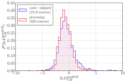
Since the injections have precessing spins while in the recovery we only allow for (anti-)aligned spins, the recovery waveform model will not perfectly capture the signal even for BNS. Nevertheless, the effect on the background distribution is minor, as shown in Fig. 6; one has . Clearly, given the relative smallness of the spins, allowing for (anti-)aligned spins in TaylorF2 is sufficient for this waveform model to capture the spin effects in the signal, at least to the extent that the background is not significantly affected.
III.7 Combined effect of differences between waveform approximants, tidal deformation, calibration errors, and spins
We now put everything together and compute a background distribution where the recovery waveform is TaylorF2 with (anti-)aligned spins, cut off at 400 Hz, but the injections are TaylorT4 with precessing spins and tidal effects at 0PN and 1PN, and calibration errors are also included. In the case of TaylorT4, the phase is only computed numerically, and tidal effects must be added in the equation for :
| (13) |
where to 1PN order Vines2011
| (14) |
For the expression of the point particle contribution to 3.5PN, with spins included up to 2.5PN, we refer to Faye2006 .
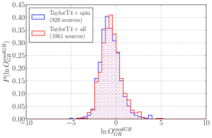
For the case of single sources, the effect on the background of a combination of precessing spins, tidal effects, and calibration errors is shown in Fig. 7. In terms of a KS statistic, the difference between backgrounds is .
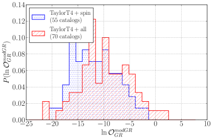
For reasons of computational expense, so far we have only shown differences between backgrounds for single sources, which is appropriate for the case where there is only one detection. If there are detections that can be clearly identified as BNS events according to the criterion , then one will want to construct a background distribution for catalogs of sources each. We computed backgrounds using the injection sets of Fig. 7, but now randomly combining injections into catalogs of 15 sources each. The results are shown in Fig. 8. When information from multiple GR sources is combined, one expects to be much more favored over , and this is what we see: in both cases, the distribution of stretches to much more negative values. However, when making comparisons of different physical set-ups, combining information from multiple sources can make the differences show up much more clearly than in the case of single sources. For the purposes of this paper, a much smaller number of simulations were performed than one would in reality; one has , but this will in large part be due to small number statistics. Reassuringly, even for catalogs of sources, the two background distributions are rather similar, with both favoring strongly negative values of log odds.
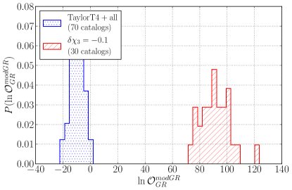
Finally, we want to show at least one example of how well violations of GR might be detectable in the presence of strong tidal effects, instrumental calibration errors, and precessing spins. Recalling that the 1.5PN contribution to the orbital motion is where, according to GR, the dynamical self-interaction of spacetime first becomes visible Blanchet1994 ; Blanchet1995 , we consider a (heuristic) violation of GR at that order, taking the form of a shift in the relevant coefficient in the expansion of :
| (15) | |||||
where we note that the leading-order contribution to goes like ; is the 1.5PN coefficient predicted by GR, and .
In Fig. 9, we show background as well as foreground log odds ratio distributions, for catalogs of 15 sources each, where in both cases the injections include neutron star tidal deformation, instrumental calibration errors, and precessing spins. As before, the recovery is with TaylorF2 waveforms that allow for (anti-)aligned spins, cut off at a frequency of 400 Hz. We see that the separation between the distributions is complete: almost regardless of false alarm probability, with 15 BNS detections the efficiency in finding the given GR violation is essentially 100%.
IV Conclusions and future directions
We have developed TIGER, a data analysis pipeline to perform model-independent tests of general relativity in the strong-field regime, using detections of compact binary coalescence events with second-generation gravitational wave detectors. The basic idea is to compare the GR hypothesis with the hypothesis that one or more coefficients in the post-Newtonian expression for the phase do not depend on component masses and spins in the way GR predicts. Though the latter hypothesis has no waveform model associated with it, it can be written as the logical union of mutually exclusive sub-hypotheses, in each of which a fixed number of phase coefficients are free parameters on top of component masses, spins, sky position, orientation, and distance, while the others depend on masses and spins in the way GR predicts. In present form, the pipeline can in principle already be applied to binary neutron star events, for which waveform models that are reliable and can be generated sufficiently fast on a computer are available.
We performed a range of numerical experiments to check the robustness of TIGER against fundamental, astrophysical, and instrumental unknowns. In the BNS mass regime, the differences between the available waveform approximants are very small, making it unlikely that imperfect modeling of the signal will cause us to suspect a violation of GR. The fact that waveforms are only known up to a finite post-Newtonian order should also not be cause for concern. In the final stages of inspiral, finite size effects are important and the neutron stars will deform each other in an essentially unknown way; however, if the recovery waveforms are cut off at 400 Hz then the unknown tidal effects will not be mistaken for violations of GR, but the performance of TIGER remains unaffected. Instrumental calibration errors of expected size will not be problematic. Finally, if, as generally expected, the spins of neutron stars in binaries are small, then they can easily be dealt with.
In present form, TIGER relies on two important astrophysical assumptions. One is that NSBH and BBH coalescences have chirp masses above a certain value, so that such events can be discarded, leaving only BNS. The other is the relative smallness of spins for BNS. In the future we will also want to work with BBH and NSBH events so that if an anomaly is discovered in BNS signals, we can confirm that it is of a fundamental rather than an astrophysical nature by using qualitatively different systems. Pan et al. appear to have arrived at a reliable semi-analytic waveform model for BBH and NSBH coalescence Pan2013 , and their approximant will be extremely useful as an injection waveform. However, it is too computationally expensive to be used for recovery. On the other hand, very recently Hannam et al. Hannam2013b proposed a frequency domain inspiral-merger-ringdown waveform which captures precessing spins, and which may already be useful for our purposes. An upgrade of the fast time domain “PhenSpin” waveform of Sturani et al. could also be an option for recovery PhenSpin1 ; PhenSpin2 . (Note that for the background calculation, it is important that the injected waveform model be as close as possible to reality, but the requirements for the recovery waveform are less stringent.) To have some idea of what might conceivably be possible with BBH, we used the earlier BBH waveform approximant of Santamaria2010 with spins set to zero, for both injection and recovery, choosing component masses to be in the range and placing sources uniformly in co-moving volume with distances up to 1.25 Gpc. It was found that for catalogs of 20 sources each, a deviation in (the equivalent of) the 3PN phase coefficient of only 0.5% could be picked up with essentially 100% efficiency, using only as testing coefficients; see Fig. 6 of VanDenBroeck2013 . Here some caution is called for, considering that astrophysical black holes are likely to have large, non-aligned spins, but the result is encouraging. The possibility of reliably applying TIGER to BBH detections using a waveform model along the lines of Hannam et al. Hannam2013b or Sturani et al. PhenSpin1 ; PhenSpin2 will be a subject of intense investigation.
Demonstrating the robustness of TIGER, applied to BNS, against fundamental and astrophysical unknowns as well as instrumental calibration errors was a necessary first step in determining whether it will be viable as a data analysis pipeline. A crucial further check will be to assess the behavior of TIGER in real noise, which is not quite stationary or Gaussian. We are in the process of testing the pipeline using existing data taken by the initial LIGO and Virgo detectors, but “recolored” so that the underlying power spectral densities are the ones predicted for the advanced interferometers, while retaining the non-stationarities in the noise. Results will be reported in a forthcoming publication.
Acknowledgements
MA, WDP, TGFL, CVDB, and JV were supported by the research programme of the Foundation for Fundamental Research on Matter (FOM), which is partially supported by the Netherlands Organisation for Scientific Research (NWO). SV acknowledges the support of the National Science Foundation and the LIGO Laboratory. LIGO was constructed by the California Institute of Technology and Massachusetts Institute of Technology with funding from the National Science Foundation and operates under cooperative agreement PHY-0757058. The authors would like to acknowledge the LIGO Data Grid clusters, without which the simulations could not have been performed. Specifically, these include the computing resources supported by National Science Foundation Grants PHY-0923409 and PHY-0600953 to UW-Milwaukee. Also, we thank the Albert Einstein Institute in Hannover, supported by the Max-Planck-Gesellschaft, for use of the Atlas high-performance computing cluster. It is a pleasure to thank E. Berti, A. ter Braack, A. Buonanno, N. Cornish, J.D.E. Creighton, W.M. Farr, B.R. Iyer, C.K. Mishra, C. Pollice, B.S. Sathyaprakash, R. Sturani, and N. Yunes for useful discussions.
References
- (1) C.W. Misner, K.S. Thorne, and J.A. Wheeler, Gravitation, W.H. Freeman and Company, New York, 1973
- (2) C. M. Will, Liv. Rev. Rel. 9, 3 (2006) http://www.livingreviews.org/lrr-2006-3
- (3) R.A. Hulse and J.H. Taylor, Astrophys. J. 195, L51 (1975)
- (4) J.M. Weisberg, D.J. Nice, and J.H. Taylor, Astrophys. J. 722, 1030 (2010)
- (5) P.C.C. Freire et al., Mon. Not. R. Astron. Soc. 423, 3328 (2012)
- (6) Antoniadis et al., Science 340, 1233232 (2013)
- (7) L. Blanchet and B.S. Sathyaprakash, Class. Quantum Grav. 11, 2807 (1994)
- (8) L. Blanchet and B.S. Sathyaprakash, Phys. Rev. Lett. 74, 1067 (1995)
- (9) G.M. Harry for the LIGO Scientific Collaboration, Class. Quantum Grav. 27, 084006 (2010)
- (10) Advanced Virgo Baseline Design, The Virgo Collaboration, technical note VIR027A09 (2009)
- (11) H. Grote (for the LIGO Scientific Collaboration), Class. Quantum Grav. 25, 114043 (2008); H Grote and the LIGO Scientific Collaboration, Class Quantum Grav. 27, 084003 (2010)
- (12) K. Kuroda for the LCGT Collaboration, Class. Quantum Grav. 27, 084004 (2010)
- (13) C.S. Unnikrishnan, Int. J. Mod. Phys D 22, 1341010 (2013); LIGO Scientific Collaboration, Technical Note No. P1200166-v1 (2012)
- (14) J. Abadie et al., Class. Quantum Grav. 27, 173001 (2010)
- (15) J. Aasi et al.; arXiv:1304.0670 [gr-qc]
- (16) H.-Y. Chen and D.E. Holz; arXiv:1206.0703 [astro-ph]
- (17) J.R. Gair, M. Vallisneri, S.L. Larson, J.G. Baker, Liv. Rev. Rel. 16, 7 (2013)
- (18) N. Yunes and X. Siemens, Liv. Rev. Rel. 16, 9 (2013)
- (19) K.G. Arun, B.R. Iyer, M.S.S. Qusailah, and B.S. Sathyaprakash, Class. Quantum Grav. 23, L37 (2006)
- (20) K.G. Arun, B.R. Iyer, M.S.S. Qusailah, and B.S. Sathyaprakash, Phys. Rev. D 74, 024006 (2006)
- (21) C.K. Mishra, K.G. Arun, B.R. Iyer, and B.S. Sathyaprakash, Phys. Rev. D 82, 064010 (2010)
- (22) S. Gossan, J. Veitch, and B.S. Sathyaprakash, Phys. Rev. D 85, 124056 (2012)
- (23) W. Del Pozzo, J. Veitch, and A. Vecchio, Phys. Rev. D 83, 082002 (2011)
- (24) N. Yunes and F. Pretorius, Phys. Rev. D 80, 122003 (2009)
- (25) N. Cornish, L. Sampson, N. Yunes, and F. Pretorius, Phys. Rev. D 84, 062003 (2011)
- (26) K. Chatziioannou, N. Yunes, and N. Cornish, Phys. Rev. D 86, 022004 (2012)
- (27) L. Sampson, N. Yunes, and N. Cornish, Phys. Rev. D 88, 064056 (2013)
- (28) T.G.F. Li et al., Phys. Rev. D 85, 082003 (2012)
- (29) K.S. Thorne, in 300 Years of Gravitation, eds. S.W. Hawking and W. Israel, Cambridge University Press, Cambridge, England, 1987
- (30) B.S. Sathyaprakash and S.V. Dhurandhar, Phys. Rev. D 44, 3819 (1991)
- (31) C. Van Den Broeck and A.S. Sengupta, Class. Quantum Grav. 24, 155 (2007)
- (32) C. Van Den Broeck and A.S. Sengupta, Class. Quantum Grav. 24, 1089 (2007)
- (33) R. O’Shaughnessy, B. Farr, E. Ochsner, H.-K. Cho, C. Kim, and C.-H. Lee; arXiv:1308.4704 [gr-qc]
- (34) F. Beauville et al., Class. Quantum Grav. 22, 4285 (2005)
- (35) D.A. Brown (for the LIGO Scientific Collaboration), Class. Quantum Grav. 22, S1097 (2005)
- (36) S. Babak, R. Balasubramanian, D. Churches, T. Cokelaer, and B.S. Sathyaprakash, Class. Quantum Grav. 23, 5477-5504 (2006)
- (37) T. Cokelaer, Phys. Rev. D 76, 102004 (2007)
- (38) T. Cokelaer, Class. Quantum Grav. 24, 6227 (2007)
- (39) C. Van Den Broeck et al., Phys. Rev. D 80, 024009 (2009)
- (40) D.A. Brown, I. Harry, A. Lundgren, and A.H. Nitz, Phys. Rev. D 86, 084017 (2012)
- (41) S. Babak et al., Phys. Rev. D 87, 024033 (2013)
- (42) D.A. Brown, P. Kumar, and A.H. Nitz, Phys. Rev. D 87, 082004 (2013)
- (43) T.G.F. Li et al., J. Phys. Conf. Ser. 363, 012028 (2012)
- (44) C. Van Den Broeck, Probing dynamical spacetimes with gravitational waves, to appear in Springer Handbook of Spacetime, eds. A. Ashtekar and V. Petkov, Springer Verlag, Berlin, 2013
- (45) J. Abadie et al., Astrophys. J. 760, 12 (2012)
- (46) https://www.lsc-group.phys.uwm.edu/daswg/projects/lalsuite.html
- (47) A. Buonanno, B.R. Iyer, E. Ochsner, Y. Pan, and B.S. Sathyaprakash, Phys. Rev. D 80, 084043 (2009)
- (48) J. Aasi et al., Phys. Rev. D 88, 062001 (2013)
- (49) M. Dominik et al., Astrophys. J. 759, 52 (2012)
- (50) S. Vitale and W. Del Pozzo, Phys. Rev. D 89, 022002 (2014)
- (51) C. Cutler et al., Phys. Rev. Lett. 70, 2984 (1993)
- (52) M. Maggiore, Gravitational Waves. Volume 1: Theory and Experiments, Oxford University Press, Oxford, 2008
- (53) J. Veitch and A. Vecchio, Phys. Rev. D 78, 022001 (2008)
- (54) J. Veitch and A. Vecchio, Class. Quant. Grav. 25, 184010 (2008)
- (55) J. Veitch and A. Vecchio, Phys. Rev. D 81, 062003 (2010)
- (56) A. Kolmogorov, G. Inst. Ital. Attuari 4, 83 (1933)
- (57) N.V. Smirnov, Ann. Math. Stat. 19, 279 (1948)
- (58) T. Hinderer, B.D. Lackey, R.N. Lang, and J.S. Read, Phys. Rev. D 81, 123016 (2010)
- (59) T. Damour, A. Nagar, and L. Villain, Phys. Rev. D 85, 123007 (2012)
- (60) J.M. Lattimer, Annu. Rev. Nucl. Part. Sci. 62, 485 (2012)
- (61) W. Del Pozzo, T.G.F. Li, M. Agathos, C. Van Den Broeck, and S. Vitale, Phys. Rev. Lett. 111, 071101 (2013)
- (62) J.S. Read et al., Phys. Rev. D 88, 044042 (2013)
- (63) P. Ajith et al., Class. Quantum Grav. 29, 124001 (2012)
- (64) L.E. Simone, S.W. Leonard, E. Poisson, and C.M. Will, Class. Quantum Grav. 14, 237 (1997)
- (65) S. Vitale et al., Phys. Rev. D 85, 064034 (2012)
- (66) D.R. Lorimer, Liv. Rev. Rel. 11, 8 (2008)
- (67) G. Faye, L. Blanchet, and A. Buonanno, Phys. Rev. D 74, 10403 (2006)
- (68) A. Bohé, S. Marsat, and L. Blanchet, Class. Quantum Grav. 30, 135009 (2013)
- (69) K.G. Arun, A. Buonanno, G. Faye, and E. Ochsner, Phys. Rev. D 79, 104023 (2009); Erratum ibid. D 84, 049901 (2011)
- (70) M. Agathos, W. Del Pozzo, T.G.F. Li, C. Van Den Broeck, J. Veitch, and S. Vitale, to appear in Proceedings of the 13th Marcel Grossmann Meeting; arXiv:1305.2963 [gr-qc]
- (71) J. Vines, T. Hinderer, and É.É. Flanagan, Phys. Rev.D 83, 084051 (2011)
- (72) Yi Pan et al.; arXiv:1307.6232 [gr-qc]
- (73) M. Hannam et al.; arXiv:1308.3271 [gr-qc]
- (74) R. Sturani et al., J. Phys. Conf. Ser. 243, 012007 (2010)
- (75) R. Sturani et al., arXiv:1012.5172 [gr-qc]
- (76) L. Santamaria et al., Phys. Rev. D 82, 064016 (2010)