Anisotropic -Gaussian 3D velocity distributions in CDM haloes
Abstract
The velocity distribution function (VDF) of dark matter (DM) haloes in CDM dissipationless cosmological simulations, which must be non-separable in its radial and tangential components, is still poorly known. We present the first single-parameter, non-separable, anisotropic model for the VDF in CDM haloes, built from an isotropic -Gaussian (Tsallis) VDF of the isotropic set of dimensionless spherical velocity components (after subtraction of streaming motions), normalized by the respective velocity dispersions. We test our VDF on 90 cluster-mass haloes of a dissipationless cosmological simulation.
Beyond the virial radius, , our model VDF adequately reproduces that measured in the simulated haloes, but no -Gaussian model can adequately represent the VDF within , as the speed distribution function is then flatter-topped than any -Gaussian can allow. Nevertheless, our VDF fits significantly better the simulations than the commonly used Maxwellian (Gaussian) distribution, at virtually all radii within . Within 0.4 (1) , the non-Gaussianity index is (roughly) linearly related to the slope of the density profile and also to the velocity anisotropy profile. We provide a parametrization of the modulation of with radius for both the median fits and the fit of the stacked halo. At radii of a few percent of , corresponding to the Solar position in the Milky Way, our best-fit VDF, although fitting better the simulations than the Gaussian one, overproduces significantly the fraction of high velocity objects, indicating that one should not blindly use these -Gaussian fits to make predictions on the direct detection rate of DM particles.
keywords:
dark matter; galaxies: clusters; galaxies: haloes; galaxies: kinematics and dynamics1 Introduction
While dark matter appears to constitute 85% of the mass of the Universe, much work is being performed to detect dark matter particles and to quantify its distribution in astronomical systems. In particular, experiments have been developed in order to detect the passage of dark matter particles through terrestrial detectors: DAMA (Bernabei et al., 2013), CoGeNT (Aalseth et al., 2013), CRESST-II (Petricca et al., 2012), CDMS-Si (Agnese et al., 2013), and Xenon100 (Aprile et al., 2012). The knowledge of the precise high-end part of the distribution of space (3D) velocities (hereafter velocity distribution function or VDF) in the inner halo, corresponding to the Solar position in the Milky Way galaxy, is required to quantify the expected event rate in direct dark matter detection experiments. Indeed, these experiments involve a detection threshold in kinetic energy, which for light (e.g. in mass) dark matter particles corresponds to velocities of order of , i.e. somewhat higher than the expected velocity dispersion of halo dark matter particles in the Solar neighbourhood. With this goal in mind, the VDF in cold dark matter (CDM) haloes has drawn attention during the last few years (Fairbairn & Schwetz, 2009; Vogelsberger et al., 2009; Ling et al., 2010; Kuhlen et al., 2010; Lisanti et al., 2011; Mao et al., 2013; Pato et al., 2013).
The knowledge of the VDF is also important for modeling the radial profiles of mass (including dark matter) and velocity anisotropy of quasi-spherical systems from the distribution of their tracers (stars in galaxies; galaxies in clusters) in projected phase space (PPS: projected radius and line-of-sight velocity). The cleanest way to perform this mass / anisotropy analysis is to model the distribution of tracers in PPS, but this requires a triple integral of the six-dimensional distribution function (DF) expressed in terms of energy and angular momentum, (Dejonghe & Merritt, 1992). For example, the method of Wojtak et al. (2009) that starts from the CDM halo DF of Wojtak et al. (2008) is very slow (requiring a day on a single processor to run for a 500-tracer system with full error sampling from Markov Chain Monte-Carlo (MCMC) methods). Orbit modeling (Schwarzschild, 1979; Richstone & Tremaine, 1984; Syer & Tremaine, 1996) is much slower, thus preventing proper error sampling by MCMC. Recently, Mamon, Biviano, & Boué (2013) have developed an algorithm called MAMPOSSt, in which the distribution of tracers in PPS is expressed as a single integral: is replaced by the distribution of line-of-sight velocities at a given (3D) position, which in turn depends on the combination of the radial profiles of the total mass and the velocity anisotropy
| (1) |
as well as a suitably simple form for the VDF. So far, MAMPOSSt has only been used with a Maxwellian (or Gaussian111We will refer to the Maxwellian VDF in the physical context, and to the Gaussian VDF in the mathematical context.) VDF (Mamon et al., 2013; Biviano et al., 2013; Munari, Biviano, & Mamon, 2014; Guennou et al., 2014; Mamon et al., 2015). However, -body simulations (both cosmological and academic ones) indicate that VDFs show departures from Gaussianity in their radial component (Wojtak et al., 2005; Hansen et al., 2006) and also their tangential component (Hansen et al., 2006). Moreover, forcing Gaussianity in the VDF of isotropic systems built from the Jeans equation of local dynamical equilibrium leads to unstable density profiles, whereas analogous systems built from distribution functions are stable (Kazantzidis et al., 2004).
The appropriate statistical mechanical description of the 6D structure of self-gravitating spherical systems is an old and still open problem. A generalization of the Maxwellian VDF has been proposed in the context of the non-extensive thermodynamics developed by Tsallis (1988). The Tsallis VDF, alternatively called -Gaussian, is equivalent to the polytropic gas model (see Plastino & Plastino, 1993), of which the isothermal sphere is a particular case. The Tsallis VDF has been applied to describe phenomena of diverse fields of physics, particularly self-gravitating systems, but also to the direct detection of dark matter particles (Vergados, Hansen, & Host, 2008).
To the best of our knowledge, all analyses of non-Maxwellian VDFs, with one exception, assume velocity isotropy (Vogelsberger et al., 2009; Lisanti et al., 2011; Mao et al., 2013), a VDF that is separable into its radial and tangential components (Hansen et al., 2006; Fairbairn & Schwetz, 2009; Kuhlen et al., 2010), or tried both (Ling et al., 2010). Recently, Hunter (2014) generalized the VDF of Mao et al. (2013) to a joint form of radial and tangential velocities, but his model involves 3 parameters.
Interestingly, the radial and tangential components of the VDF of structures in cosmological and academic -body simulations are well fit, separately, by the -Gaussian formula (Hansen et al., 2006), although other modifications to the Gaussian have been shown to also fit well the VDFs of haloes (at the solar radius, Fairbairn & Schwetz, 2009; Kuhlen et al., 2010; Lisanti et al., 2011; Mao et al., 2013). Moreover, simulations of both collapsing structures and cosmological haloes indicate that for both for the radial velocity and the tangential velocity distributions, the parameter of non-Gaussianity is found to vary roughly linearly with the slope of the density profile for radii where the slopes are between –2.7 and –1 (Hansen et al., 2006). Finally, Hansen & Sparre (2012) demonstrate that the tangential VDF must scale, outside its wings, as at all radii.
In fact, were the dynamical evolution of these systems just determined by two-body interactions, as is the case for ideal gases, i.e., if the two-body relaxation time were short, then the system would rapidly evolve to isotropic velocities in a short time scale, the distribution function would then depend solely on energy, , and could be obtained from the density profile (Eddington, 1916), and finally, the velocity modulus distribution function at radius would then simply be . However, in most large-scale astronomical systems (galaxies and clusters), the two-body relaxation time of the dark matter component is longer than the age of the Universe. One might still expect that violent relaxation, caused by a rapidly varying gravitational potential (Lynden-Bell, 1967), will redistribute energies and lead to a possibly stationary configuration. However, violent relaxation is not thought to be long-term, and, furthermore, the energies are not completely redistributed (Madsen, 1987; Kandrup, Mahon, & Smith, 1993; Beraldo e Silva et al., 2014).
On the other hand, simulations and observational modeling suggest that the VDF in elliptical galaxies and galaxy clusters is most likely anisotropic. Indeed, CDM haloes of cluster-mass haloes show radial velocities at outer (e.g., Lemze et al., 2012) or all (Wojtak, Gottlöber, & Klypin, 2013) radii. Moreover, dynamical studies of galaxies (Wojtak & Mamon, 2013) and clusters (Biviano & Katgert, 2004; Łokas et al., 2006; Wojtak & Łokas, 2010; Biviano et al., 2013; Munari et al., 2014) point to radial outer velocity anisotropy.
In principle, the VDF can be deduced from the DF. For anisotropic spherical systems, since , the VDF at radius will be
| (2) |
For example, one could use the separable form of the DF that Wojtak et al. (2008) measured for CDM haloes. However, that DF involves a total of 8 parameters, so, although interesting, the approach of equation (2) is left for future work (see also Fornasa & Green, 2014).
The separability of the DF in energy and angular momentum thus indicates that the VDF of CDM haloes is a non-separable function of radial and tangential velocities. Indeed, if , then according to equation (2), cannot be separated from within , unless , where is a constant, but this is not the case for CDM haloes (Wojtak et al., 2008).
Thanks to the interest in direct dark matter detection, most work on the VDF has been restricted to radii of percent of the virial radius, , i.e. the position of the Earth in the halo of the Milky Way. On the other hand, as in many other mass / velocity anisotropy modeling methods, MAMPOSSt involves integrals along the line-of-sight (LOS), corresponding to physical radii extending from to infinity, in principle. In practice, the Hubble flow stretches the velocity vs. distance-to-halo-centre relation so that beyond , the line-of-sight velocities extend beyond (e.g., Mamon, Biviano, & Murante, 2010). Thus, the knowledge of the VDF is required at all radii from the halo centre to .
In this work, we propose the first anisotropic VDF for CDM haloes that is a non-separable function of radial and tangential velocities, after that of Hunter (2014). Our VDF is an extension of the -Gaussian VDF to spherical systems with anisotropic velocities. Instead of 3 parameters as in the Hunter VDF, ours has only one parameter: the non-Gaussianity index . We do not advocate any fundamental basis for the -Gaussian velocity distribution. Instead, we treat it as a powerful parametrization that allows us to phenomenologically describe systems whose 3D velocity distributions depart from the Gaussian distribution. We then fit our anisotropic -Gaussian model to the VDF of simulated CDM haloes, between 0.03 and , to check if it provides a significantly better representation of the VDF than does the Gaussian model with one parameter less.
Note that this non-separable form of the VDF has the practical advantage that it is straightforward to compute the distribution of line-of-sight velocities from it, while the distribution of line-of-sight velocities for a separable -Gaussian VDF cannot be expressed in analytical form in a single quadrature. This means that this non-separable -Gaussian VDF can be incorporated into the MAMPOSSt mass/orbit modeling technique.
In Sect. 2, we review the classical and simplest case, of the Gaussian velocity distribution from the Maxwellian approach. In Sect. 3, we present the -Gaussian velocity distribution and briefly describe its extensions to thermodynamics. Then, in Sect. 4, we generalize the -Gaussian velocity distribution to spherical systems with anisotropic velocities. In Sect. 5, we describe the simulated data that we use, while in Sect. 6 we explain how we arrange the data and fit the non-Gaussianity index. In Sect. 7, we analyze the properties of the 3D velocity distribution of cluster-mass CDM haloes as a function of radial distance to the halo centre. We discuss our results in Sect. 8.
2 Gaussian velocity distribution
The velocity distribution of an ideal gas in equilibrium was first determined by Maxwell (1860), based on two symmetry hypotheses (see Sommerfeld, 1993; Silva, Plastino, & Lima, 1998; Diu et al., 2007):
-
1.
The velocity distribution is isotropic. This implies that .
-
2.
The 3 directions are statistically independent. This, using cartesian coordinates, implies that , where , and can be different in general.
Together, these hypotheses imply that
| (3) |
Following standard steps, from eq. (3) we write
| (4) |
and differentiate both sides relative to , obtaining
| (5) |
In equation (5), the left-hand side is only a function of , while the right-hand side is only a function of , which implies that both are equal to some constant . This leads to
| (6) |
Equation (6) also holds for and . Therefore, the joint velocity distribution is
| (7) |
where is determined by the normalization condition
| (8) |
while , with the one-dimensional velocity dispersion determined by the 2nd velocity moment condition
| (9) |
3 Tsallis (or q-gaussian) velocity distribution
The DF of isotropic spherical systems implied by equation (7) is then . Since the joint assumptions of isotropy (i) and separability of the velocity components (ii) lead to purely exponential energy distributions, then non-exponential energy distributions of isotropic systems will necessarily lead to the non-separability of the VDF. For example, if the DF is truncated because of escaping particles (e.g., King, 1966), the VDF will be non-separable. This provides a natural motivation to explore non-Maxwellian VDFs such as the Tsallis distribution.
Historically speaking, the -Gaussian velocity distribution was derived in the opposite order. Firstly, a generalized version of the Boltzmann entropy was proposed by Tsallis (1988), and then the VDF was obtained by maximizing this Tsallis entropy (Plastino & Plastino, 1993). Finally, the same velocity distribution was obtained (Silva et al., 1998) following symmetry arguments similar to that of Maxwell.
In fact, assuming the velocity isotropy hypothesis (i) above — which allows us to write — but abandoning the coordinate-independence hypothesis (ii), Silva et al. (1998) proposed, as a generalization of the joint Maxwellian distribution (equation 3), the expression
| (10) |
where
is called the -exp function, and follows as , while
is called the -log function, and follows as . One can easily check that . Then, in the limit , the joint velocity distribution of equation (10) tends to the Maxwellian distribution. Following the same steps as for the Maxwellian VDF, we arrive at
| (11) |
where the constants and are obtained using the normalization equations (8) and (9) (see Silva & Alcaniz, 2003)
| (12) |
where222This value of is different from what would be inferred from eq. (7) of Silva & Alcaniz (2003), who compute the second velocity moment as instead of as in the left-hand-side of equation (9). We are using the -Gaussian VDF of equation (11) as an empirical model and are not considering the effects of the non-extensive thermodynamics proposed by Tsallis (1988), hence our use of a classical 2nd velocity moment to derive .
| (13) |
This value of imposes the tighter restriction . Note the velocity limit of when . The shape of depends on the value of . While is Maxwellian for , it has a flatter top and is sharply truncated for and has a cuspier top with wider wings when .
4 Anisotropic Tsallis (q-gaussian) velocity distribution
The velocity distribution of equation (11) depends only on the modulus of the velocity, hence is isotropic, as expected by construction. Since simulated astrophysical systems have anisotropic velocities, we now extend the -Gaussian velocity distribution to anisotropic velocities.
One possible approach to extend the -Gaussian VDF to anisotropic velocities would be to maximize the Tsallis entropy, as done by Plastino & Plastino (1993), but with additional constraints (see Stiavelli & Bertin, 1987). Instead, inspired by eq. (11), and concerned with spherically symmetric self-gravitating systems, and correcting for streaming motions (e.g., streaming radial motions beyond the virial radius), we introduce the anisotropic -Gaussian VDF as
| (14) | |||||
where the and are respectively the mean streaming velocities and velocity dispersions in the direction of the spherical coordinate system, while and are constants (dependent on ) that we shall determine below.
Defining the dimensionless normalized velocities as
| (15) |
and noting that the Jacobian relating the to the is , equation (14) can equivalently be written
| (16) |
One notices that the vector field is isotropic by construction. Equations (8) and (9) become
| (17) | |||||
| (18) |
Equation (16) is identical to equation (11) with taken from equation (13), once one sets in the latter equation to unity. Therefore,
| (19) |
and
| (23) | |||||
Considering the radial and tangential dimensionless normalized velocities
| (24) | |||||
| (25) |
the probability distribution function of is then
| (26) | |||||
The VDF expressed in dimensionless normalized velocities in equation (26) is clearly not separable into two terms respectively depending on and on .
4.1 Velocity modulus (or speed) distribution
As for the Maxwellian VDF, it is interesting to define the probability distribution function of the modulus of the velocity, i.e. the speed distribution function (SDF) of the -Gaussian VDF. Defining the dimensionless normalized speed as
| (27) |
the SDF is
| (28) | |||||
where equation (16) is used for the second equality. Again, we have a maximum velocity for , which is now .
5 Simulations
To test the performance of the VDF of equation (14), we have analyzed a cosmological dark matter -body simulation performed with Gadget-2 (Springel, 2005). The simulation was run with particles in a periodic box of comoving size , using a WMAP7 cosmology: , , , . The particle mass is . The Plummer-equivalent force softening is 5% of the mean inter-particle distance and kept constant in comoving units. This amounts to . Initial conditions have been generated using the MPgrafic code (Prunet et al., 2008).
Haloes were extracted with HaloMaker 2.0 using a Friends-of-Friends technique (Davis et al., 1985), with linking length (in units of the mean interparticle separation).
We selected 90 haloes from the output of the cosmological simulation, divided in 3 subsamples of comparable mass: the first subsample contains the 30 most massive haloes, while the other two subsamples contain haloes with geometric mean differing by 0.5 and by 1.0 dex from the geometric mean of the first subsample (i.e., the haloes of mass rank and ).
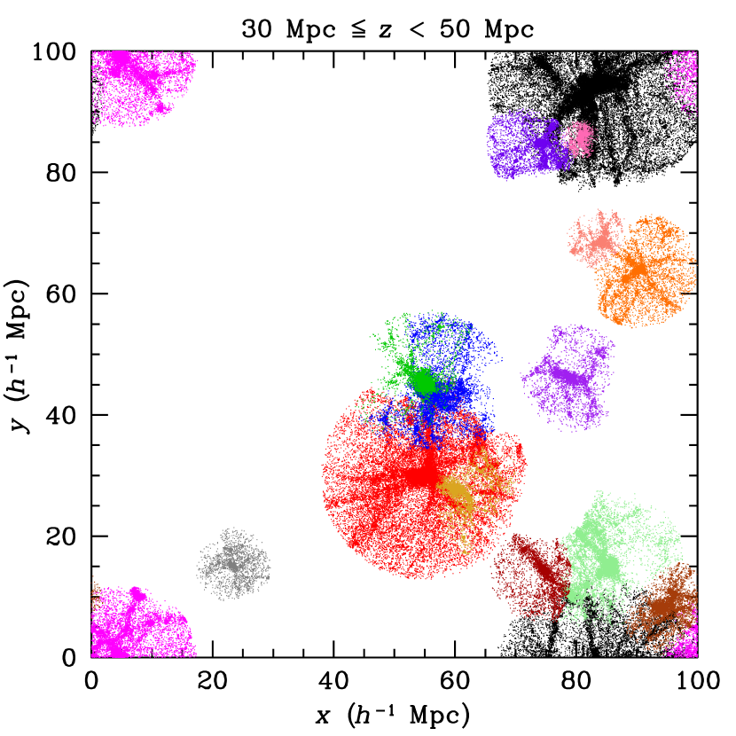
We analyzed the haloes as follows (taking into account the periodic boundary conditions at all steps). First, we refined the centre of each of the 250 most massive haloes using an iterative median centre scheme, starting on the halo particles returned by the halo finder, computing the median halo coordinates, and restricting to the particles within half of the initial (virial) radius around the new centre, iterating 3 times (each within smaller regions). We then re-estimated the virial radii of the 250 most massive haloes by finding the radius, , where the mean density within the sphere centered on the newly determined centre is 100 times the critical density of the Universe at .333For the cosmology of our simulation the mean density within the virial radius is 97 according to the approximation of Bryan & Norman (1998). For this, we considered all radii out to 3 old virial radii from the newly determined centre and solved for .
For our three subsamples of haloes, the median virial masses are then , , and , in each of the three subsamples, respectively. The corresponding median virial radii are , 1.02, and , the softening length of the simulation is 0.010, 0.014, and 0.020 times these respective virial radii, and the median number of particles within these virial radii are , and , respectively.
To avoid assigning particles outside of halo virial spheres to two or more haloes, we reassigned all particles to the nearest of the 250 most massive haloes in units of their virial radii. Fig. 1 illustrates the procedure. One notices that some haloes are cut by other haloes among the that are not shown, as for example seen in the left-lower-left part of the orange halo centered near .
6 Fitting procedure
We performed two types of analyses. On one hand, we split each of the 90 haloes into radial bins of particles (where the radii of each halo were normalized to the virial radius of that halo), and then normalized the 3 spherical velocity coordinates by subtracting the mean and dividing by the dispersion, as in equation (15). For each halo, we fit for vs. (see last paragraph of this section). We then performed linear interpolation (without extrapolation) of and other parameters on a grid of 27 geometrically-spaced radii, from to 1.1 in steps of 0.1, i.e. from (within which the definition of the centre and the softening length of the simulation may affect the results) to (beyond which the Hubble flow moves the LOS velocities beyond , see Sect. 1). This allowed us to determine the median values (over haloes) of in fixed radial bins.
On the other hand, we built a stacked halo, with all particles of our 90 haloes. We considered all 90 haloes together, using the normalized radii computed for the individual haloes (see above). Within 175 radial bins of equal numbers () of particles, we normalized the 3 spherical velocity coordinates as for the individual haloes (again using equation 15). In the end, our stacked halo contained 52 351 250 particles out to , with radii normalized by and dimensionless velocities , and . We then fit on either the 175 equal number radial bins or on the 27 geometrically spaced radial bins.
The maximum likelihood estimate of can be determined from the distribution of , by minimizing
| (29) |
where is given in equation (26) and depends on . We have minimized, instead,
| (30) |
where is given in equation (28), and the extra term is independent of , hence minimizing is equivalent to minimizing . The minimization was performed using the simulated annealing method on the values.
7 Results
7.1 Radial profiles of non-Gaussianity
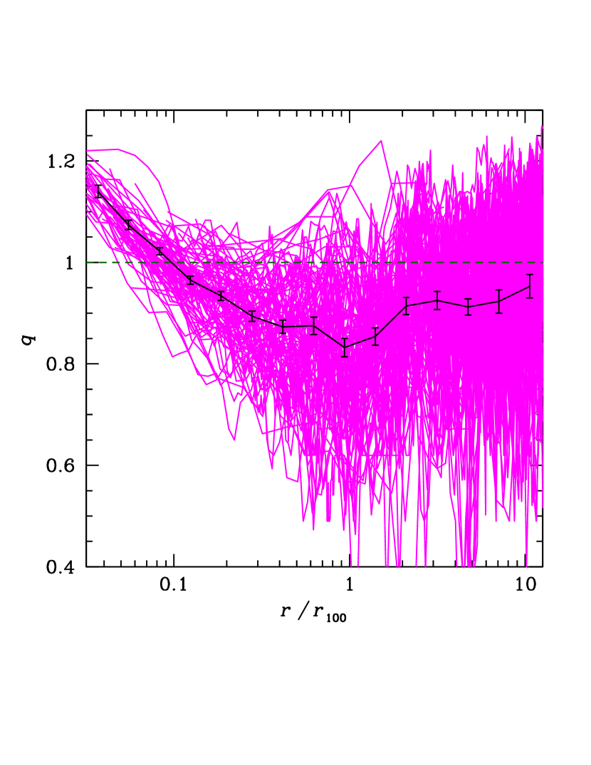
Fig. 2 shows the best-fit of our anisotropic model (equation 28) versus distance from the halo centre for the 90 individual haloes. In this work, all fits of to the distribution of are performed by maximum likelihood estimation. No halo exhibits a Gaussian444By Gaussian, we refer to the limit of our anisotropic -Gaussian model, not to be confused with the isotropic Gaussian of Sect. 2. behaviour at all radii. The non-Gaussianity index starts above unity, decreases to unity at typically , keeps decreasing to at , then rises rapidly to at , where it reaches a plateau.
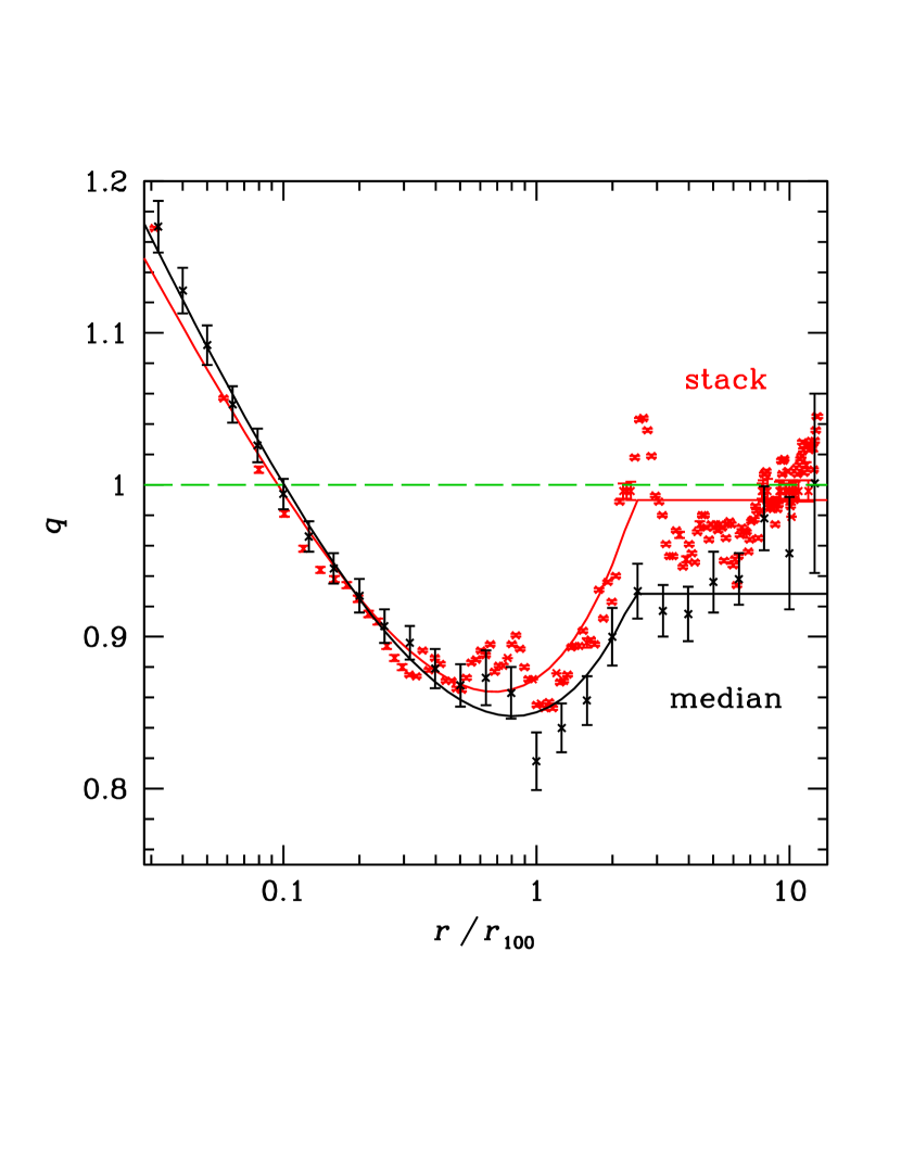
Fig. 3 shows the best fit values of obtained in the stacked halo as well as the median of individual haloes (see Sect. 5). We can see how changes in comparison to the Gaussian case of (plotted as a dashed horizontal line). We note that in the inner region, while it rises approximately as some power of at larger radii, until it reaches a plateau near unity.
This behaviour of can be described with the following 5-parameter analytical function:
| (31) | |||||
| (32) |
In equation (31), is the limit of when , is close to the power of in the rising portion of , while in equation (32) is where is minimized at , and , such that reaches its plateau at .
The continuous lines in Fig. 3 show the result of this fit. Table 1 shows the values of the parameters obtained in the “stack” and “median” cases.
| Method | |||||
|---|---|---|---|---|---|
| Stack | 0.331 | 0.757 | 0.683 | 0.864 | 2.45 |
| Median | 0.384 | 0.620 | 0.807 | 0.848 | 2.44 |
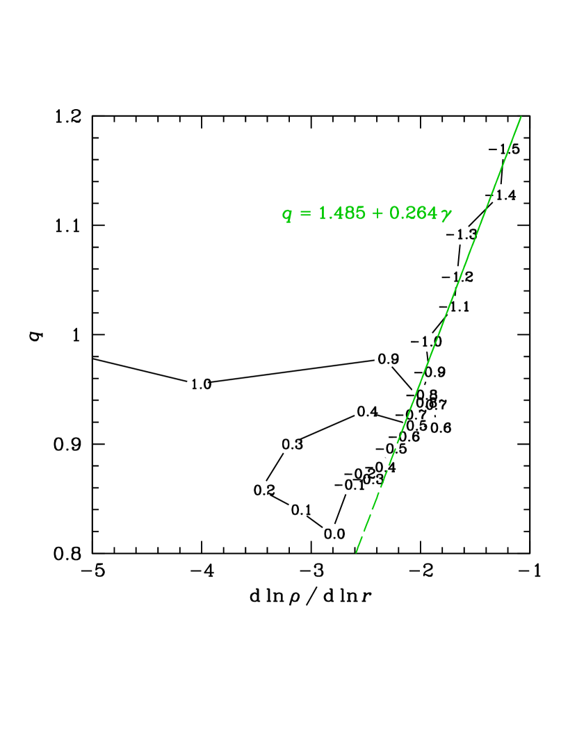
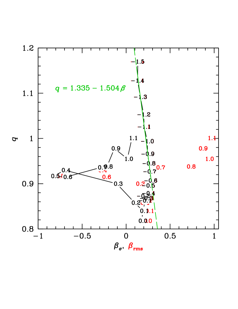
Interestingly, as shown in Fig. 4, the non-Gaussianity index of our 2D velocity model (equation 26) is linearly related to both the logarithmic slope of the density profile, , and to the velocity anisotropy . This agreement is quasi-perfect for radii (), very good for (), and decent up to the virial radius. Figure 4 is for the median properties of the 90 haloes. For the stack of the 90 haloes, the analogous figure is similar, but with a faster divergence from the linear relation starting at .
The linear relation between and confirms the linear trend of non-Gaussianity with density slope previously suggested by Hansen et al. (2006) for the radial and tangential components of the velocity distribution, although here the linearity is confined to (for a precise linearity, and up to the virial radius for approximate linearity).
We also find linear trends of with velocity anisotropy, using two different measures of velocity anisotropy, the one (hereafter ) using velocity dispersions (equation 1), and the one using rms velocities, . Note that both measures of anisotropy, and , diverge from one another only beyond the virial radius, where radial streaming motions become important.
7.2 Goodness-of-fit
We now ask whether the best-fit -Gaussian model provides an adequate representation of the simulated data.
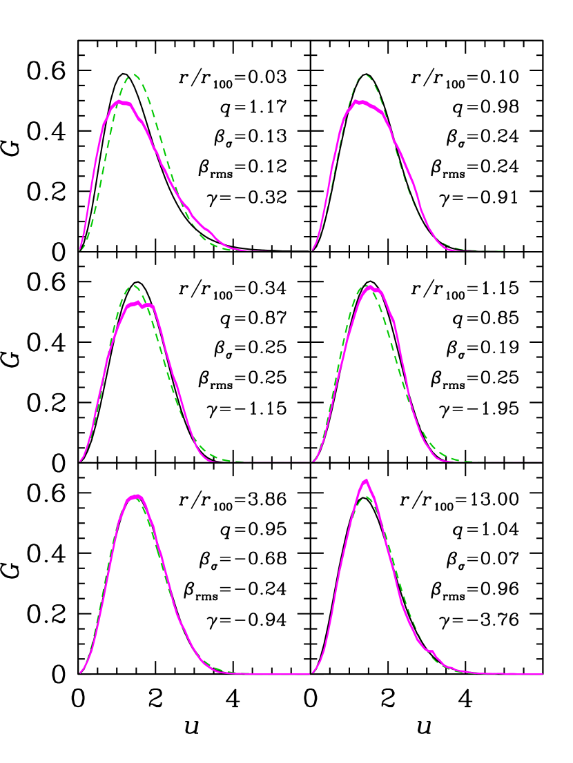
Fig. 5 displays the distribution of dimensionless normalized SDFs measured in the simulated haloes in the stacked case as well as the best fit Gaussian and -Gaussian SDFs. The dimensionless normalized SDF reaches its mode at low normalized velocity modulus at low radii () at “normal” values at the virial radius and , and at super-normal values at very high radii ().
We see that within (upper and middle-left panels of Fig. 5), the -Gaussian does not describe well the data (nor does the Gaussian, since it is a special case of the -Gaussian). For example, at , while the -Gaussian with fits the data better than the Gaussian (mostly in the low-end tail of ), its predicted velocity distribution is too peaked, and it presents an important excess of very high () velocities. These two characteristics are also present at . On the other hand, the non-Gaussian model fits well the SDF of the simulations near the virial radius, while the Gaussian model fits much less well. At 4 virial radii, both the Gaussian and non-Gaussian models fit well the simulated SDF.
Interestingly, the flattening of the SDF near its mode (i.e. flat top SDF) appears to be related to radius and slope of the density profile, as it is most prominent at small radii and shallow density slopes, while it appears unrelated to the velocity anisotropy.
A quantitative measure of the goodness-of-fit can be obtained by the Kolmogorov-Smirnov (KS) test of the maximum absolute difference between the cumulative distribution functions (CDFs) of the predicted and the simulated dimensionless normalized speeds. Given the large number of points in each radial bin of the stacked sample (), the probability that the -Gaussian model is an adequate representation of the data is rejected at over 95% confidence if the maximum absolute difference between the cumulative distribution functions of the model and the data is above 0.0025.
As we shall see below, the KS test rejects both Gaussian and non-Gaussian models, at virtually all radii for the stacked halo and at all radii when considering the median of the individual haloes.
Nevertheless, given that we have roughly equal numbers of particles per radial bin in both cases, we can illustrate the result of the KS test by plotting the maximum absolute difference in the CDFs.
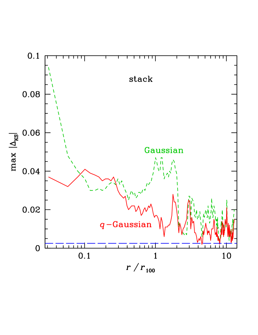
Figure 6 shows that when the KS test is applied to the stacked halo, the -Gaussian model leads to a better representation of the distribution of than does the Gaussian model, at small radii () and near the virial radius. Of course, given its extra parameter, one expects the -Gaussian to perform at least as well as the Gaussian (it can occasionally perform slightly worse, because the KS test does not measure the agreement between model and data in the same way as maximum likelihood estimation. As mentioned above, the non-Gaussian model can nevertheless be rejected with 95 percent confidence, except for two radii (out of 175, where the red line passes below the blue horizontal dashed line).
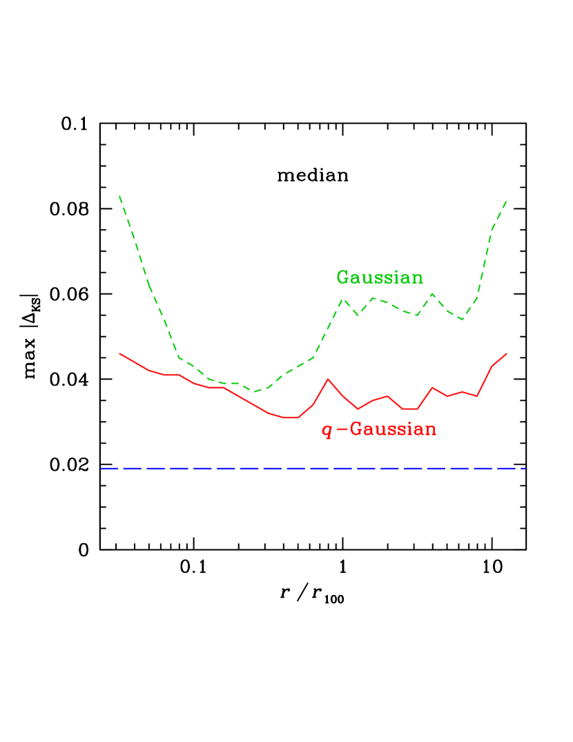
Fig. 7 shows the median KS test results over 90 haloes, i.e. the median value of the 90 maximal absolute differences in the CDFs. One sees that the -Gaussian fits are typically better not only at small radii (), and near the virial radius, but also at all radii above the virial radius. Nevertheless, as mentioned above, the -Gaussian model is typically rejected (from the median value of max ) with over 95 percent confidence at all radii.
We will check in Sect. 7.3 below whether the smaller discrepancies for the -Gaussian model (with the simulated data) in comparison with those of the Gaussian CDF are statistically significant, given the extra parameter of the non-Gaussian model.
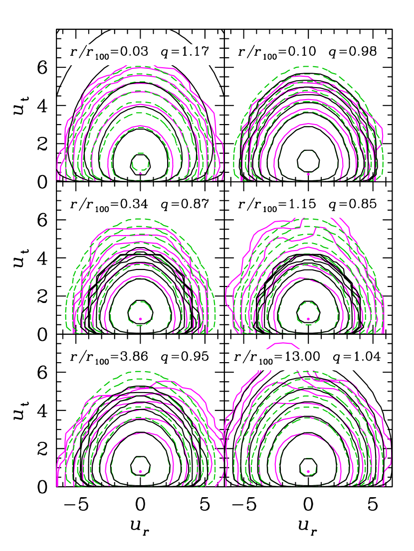
Another way to qualitatively evaluate the goodness-of-fit is to observe the contours for the 2-dimensional velocity distribution defined by the radial and tangential components. This is shown in Fig. 8. While the basic shapes of the contours of the models match fairly well the contours of the simulated data, there are differences, in the shapes, and, more strikingly, in the extent of the contours.
At , the contours of the best-fit -Gaussian extend to much greater combinations of and , i.e. to greater dimensionless normalized speeds. This is another sign that the -Gaussian predicts much more very high velocity objects than is seen in the simulation. The better fit of the -Gaussian in comparison with the Gaussian is caused by the difference in the low-end tail () of for these two cases (see upper left panel of Fig. 5), which is difficult to distinguish in the contours. At , the best-fit value of is near unity, so the contours of the Gaussian and -Gaussian are identical. Moreover, they are quite similar to the contours extracted from the simulated data (magenta), indicating that the high-end of the VDFs are similar (see upper-right panel of Fig. 5). At and , the data contours are more extended in both and than the best-fit -Gaussian. This occurs at very high speeds () and is difficult to see in the SDF (Fig. 5). At , the contours of the best-fit -Gaussian model matches those of the data for the tangential velocities, but the data contours extend to greater absolute radial velocities. Finally, at , the contours of the best-fit -Gaussian model match fairly well the data contours.
At all radii, the most probable pair of is at lower tangential velocity than predicted by the -Gaussian and Gaussian models, and low tangential velocities at high absolute radial velocities are not avoided contrary to the model predictions (near , the model contours move inwards while the data contours do not).
7.3 Does the -Gaussian model reproduce the data significantly better than the Gaussian?
We now ask whether the -Gaussian provides a significantly better fit to the simulation data than does the Gaussian, taking into account the extra parameter involved in the former. For this, we evaluated two measures of Bayesian evidence,555In the published version, equations (33) and (35) contained typographic errors, with erroneous ‘ln’ terms in front of . the Akaike Information Criterion (AIC, Akaike, 1973),
| (33) |
corrected for finite sample size by Hurvich & Tsai (1989), to yield the corrected Akaike Information Criterion (AICc) as
| (34) |
as well as the Bayes Information Criterion (BIC, Schwarz, 1978),
| (35) |
For AIC, AICc and BIC, the probability that one model is better than another is , where IC is the difference between two fits of any of the three information criteria (Kass & Rafferty, 1995). Thus, one can conclude that one model is superior to the other with 95% confidence if its value of IC is greater than the IC of the other model. Comparing equations (33) and (35), one easily sees that BIC penalizes more the extra parameter(s) in the presence of large data sets. The choice between AICc (or AIC) and BIC is still debated (Burnham & Anderson, 2004; Trotta, 2008). However, for our purposes, the results are extremely similar, so we will only display BIC for clarity.
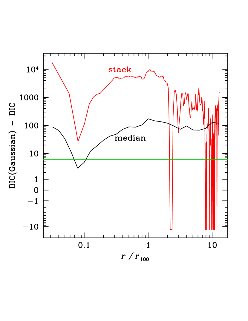
Fig. 9 shows that there is strong evidence that the -Gaussian is preferable to the Gaussian distribution for the stacked halo (red line), except, of course, at the points where , where the addition of the index is not necessary. For the median of the fits to the 90 haloes (smoother black line), we have strong evidence in favor of the -Gaussian at all radii. However, with a finer grid we would necessarily find no evidence in favor of the -Gaussian at , where .
7.4 Mass dependence
We now investigate a possible dependence of the index on the mass of the haloes. To do this, we divide our sample into the 3 mass subsamples of 30 haloes each (see Sect. 5).
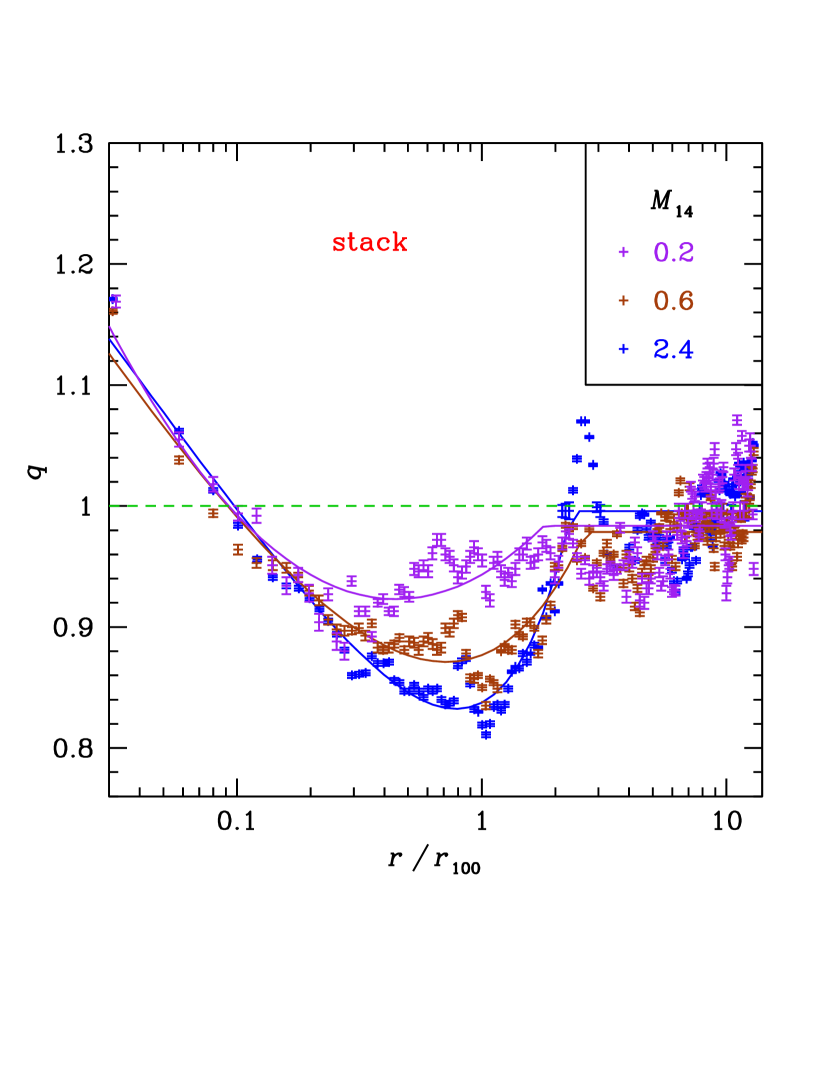
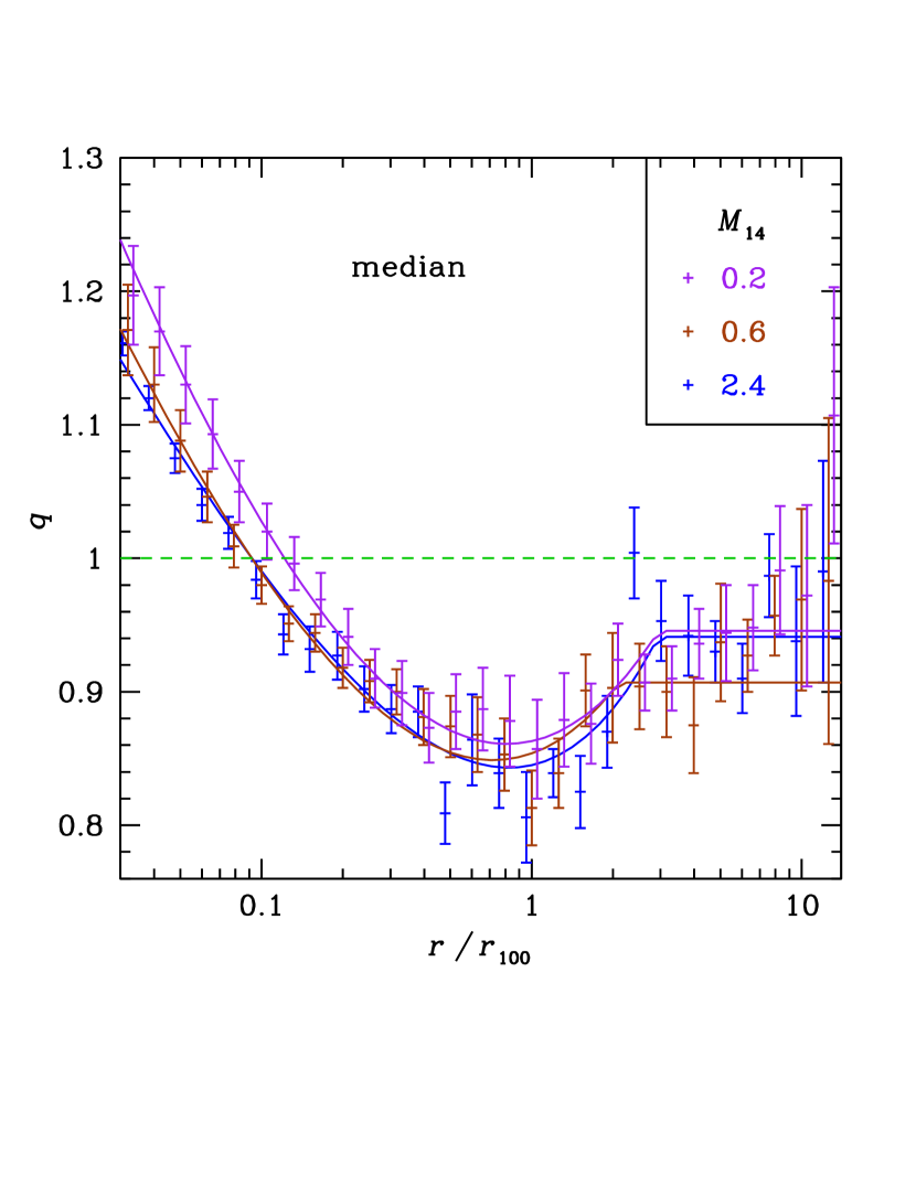
For each of these 3 subsamples, we performed the same fit procedure as before, for the stacked halo and the individual haloes, to which we consider the median fit. Fig. 11 shows that the profiles of the 3 stacked haloes show reasonable differences at intermediate radii (): The minimum is lower for the highest mass bins and this minimum is reached at progressively larger radii (in units of the virial radius). This is confirmed by the fits of the analytical function of equations (31) and (32) to the measured , as provided in Table 2.
On the other hand, Fig. 11 indicates that the 3 subsamples produce very similar median profiles (see the parameters of the analytical function fit to the median listed in Table 3). The minimum is again lower for increasingly higher halo masses, but this modulation is much weaker than for the stacked haloes: the analytical fits indicate that the differences in between the highest and lowest mass bins is only 0.018 for the median fits in comparison with 0.091 for the fits to the 3 stacked haloes.
| 0.279 | 1.329 | 0.787 | 0.832 | 2.33 | |
| 0.318 | 0.662 | 0.715 | 0.871 | 2.65 | |
| 20.257 | 0.0071 | 0.446 | 0.923 | 1.80 |
Notes: Values are for the 3 mass subsamples, whose median is indicated in the first column.
| 0.393 | 0.553 | 0.822 | 0.843 | 2.93 | |
| 0.597 | 0.344 | 0.720 | 0.849 | 2.10 | |
| 0.813 | 0.256 | 0.810 | 0.861 | 2.95 |
Notes: Values are for the 3 mass subsamples, whose median is indicated in the first column.
8 Conclusions and Discussion
In this work, we propose, for the first time, a model of the velocity distribution function for CDM haloes that is non separable in its radial and tangential components and only involves a single free parameter: it is an anisotropic version of the -Gaussian velocity distribution, given by equation (14), or equivalently equations (16), (26) or (28), which is built on an isotropic dimensionless normalized velocity field . Our VDF involves a single dimensionless normalized velocity, the modulus of , which can be written (for negligible streaming motions expected with the virial radius)
| (36) |
(see equations 1 and 27), and a single value of non-Gaussianity. In other words, at a given radius , the velocity distribution function is a function of instead of for the isotropic distribution. We find this parametrization preferable to one that is separable in the radial and tangential coordinates, as the latter is inconsistent with the separable DF of CDM haloes (Wojtak et al., 2008), although nothing guarantees that our anisotropic VDF does not violate the Jeans theorem. Our one-parameter VDF is also simpler to handle than the 3-parameter VDF of Hunter (2014), both of which are the only VDFs proposed so far involving both radial and tangential velocities in an anisotropic fashion.
We test this anisotropic -Gaussian VDF by fitting the non-Gaussianity index at different radii of simulated haloes in two ways: fitting after stacking all the selected haloes or fitting individual haloes and calculating the median value of in each radial shell. We find that nearly all haloes show decreasing with radius, from above unity at very small radii to lower than unity near the virial radius. At low radii (), the median is linearly related to both the logarithmic slope of the density profile and the velocity anisotropy, and this trend remains nearly linear up to the virial radius (Fig. 4). Above the virial radius, both the median and the of the stacked halo rise again to near unity and remain at that value up to the largest radii we analyzed (), see Figs. 2 and also 3.
The anisotropic -Gaussian predictions cannot match the simulated data in a statistically significant way (Figs. 6 and 7). The speed distribution functions of haloes have flatter tops at low radii () than the model predictions, and cuspier tops at very high radii (), see Fig. 5. The models cannot produce too few very high speeds at intermediate radii (0.34 and ), but too many high speeds at very low radii (), see Fig. 8.
Nevertheless, the anisotropic -Gaussian is highly preferred to the Gaussian distribution at nearly all radii, even when taking the extra parameter of the former into consideration (Fig. 9).
We provide appropriate expressions to describe the behaviour of the best values of as a function of the distance to the centre (Tables 1–3). These expressions can be used either to model individual haloes (the median case) or to model stacked haloes.
The linear relation of decreasing with increasing velocity anisotropy parameter (lower panel of Fig. 4) confirms the radial trends of and radial kurtosis up to 2 virial radii seen in fig. 3 of Wojtak et al. (2005). One may wonder whether the linear relation between and can be explained from first principles. Our results are in line with the combination of 1) increasing linearly with decreasing density slope found for the radial VDF by Hansen et al. (2006) (at radii where the density profile has a slope shallower than , roughly the virial radius) and 2) the wide-wing tangential VDF found by Hansen & Sparre (2012), which could be assimilated to a -Gaussian with constant . Our linear relation follows naturally from the linear relation at these radii (Hansen & Moore, 2006), and our linear relation.
Still, the origin of the relation is not clear. Our VDF is isotropic when expressed in terms of the dimensionless velocities obtained after subtracting the mean velocities and dividing by the dispersions. So our VDF ought to be independent of the velocity anisotropy.
The radial profile of of the stacked halo follows the median profile at low radii, but reaches somewhat greater values at large radii than the median of the 90 individual haloes: with asymptotic values near 0.99 for the stack versus 0.93 for the median of the individual fits (Fig. 3). This small difference may be due to a geometrical effect produced in the stacking process. Indeed, haloes in CDM cosmological simulations are triaxial (e.g., Jing & Suto, 2002), but our stacking was done without previously rotating the haloes to align their principal axes. So the stacked profile is estimated by analyzing a spherically symmetric system, while the median profile is the median of individual triaxial systems (analyzed in concentric spherical shells). Moreover, the velocity ellipsoids of simulated haloes are aligned with their density ellipsoids (Wojtak et al., 2013), which should also affect the measure of in concentric spherical shells. However, the triaxiality of cosmologically simulated haloes is strongest in the inner regions (Jing & Suto, 2002; Schneider, Frenk, & Cole, 2012), and the alignment of the velocity ellipsoid with the density ellipsoid is weakest near the virial radius (Wojtak et al., 2013). One would therefore expect that the departure of the stack and median profiles would be greatest in the inner regions of haloes. Instead, it would be worthwhile testing these ideas by stacking the haloes along their principal axes before measuring in either circular or elliptical annuli, but this is beyond the scope of this work. In any event, the analysis of the randomly stacked halo is useful for comparisons with observational studies that stack randomly (without aligning first the principal axes) quasi-circular astronomical systems (e.g., McKay et al., 2002; Prada et al., 2003; Conroy et al., 2007; Klypin & Prada, 2009; Wojtak & Mamon, 2013 for probing SDSS galaxy haloes with the kinematics of their satellites).
Cluster-mass haloes are currently merging, hence not very relaxed. On the other hand, galaxy-mass haloes have assembled their mass much earlier and are more relaxed at . Could more relaxed regions lead to closer to unity? While there is considerable scatter () between the profiles of individual haloes (Fig. 2), there is little modulation with mass (Fig. 11), in the 1 dex cluster-mass range studied here.
One should not over-interpret the results of our -Gaussian fits to small radii, such as , close to the expected position of the Sun in the Milky Way’s halo. Indeed, the best-fit -Gaussian model strongly over-predicts the fraction of objects with velocities greater than (Fig. 8). If the threshold for direct dark matter detection is that high, then the best-fit -Gaussian model will strongly over-predict the dark matter detection rate.
It is interesting to compare our results at to those obtained by other workers. Ling et al. (2010) found that the SDF of the dark matter in their hydrodynamical cosmological simulation was well fit by a -Gaussian with (after translating from their formula with exponent to our exponent of ). Hence, their SDF is more truncated than the Gaussian, while our SDF with (both stack and median) is less truncated than a Gaussian. Lisanti et al. (2011) also find SDFs that are more truncated at large velocities than the best-fit Gaussian (see their Fig. 3). In comparison, the top left panel of Fig. 5 also shows that the simulated SDF is flatter than the best-fit Gaussian model, and falls off faster at large . The preference for the Tsallis model comes from the low-end half of the SDF. Our result is robust, as none of our 90 haloes has at (Fig. 2, although a half-dozen haloes have too few particles for reliable determinations at this radius). Also, for our lower mass haloes, this radius is only 1.5 times the softening length of the cosmological simulation, so softening effects may play a role.
The differences between our results and those of previous authors might be explained by the different behaviour of the radial and tangential VDFs: at the small radius corresponding to the Solar radius in the Milky Way halo, Fairbairn & Schwetz (2009) and Kuhlen et al. (2010) find more truncated than Gaussian radial VDFs but more extended than Gaussian tangential VDFs, as Hansen & Sparre (2012) also found at all radii where the density slope satisfied . Our anisotropic VDF (and our SDF) involve some averaging between the radial and tangential components: (see equation 36). It would be worthwhile to redo the analysis presented here using equation (2) on the separable DF that Wojtak et al. (2008) measured on simulated CDM haloes.
Finally, the analysis presented here indicates that it is not optimal to assume Gaussian 3D velocities, as currently implemented in MAMPOSSt. The inclusion of our anisotropic -Gaussian VDF (equation 14) into MAMPOSSt would improve the mass / anisotropy modeling of this algorithm, for example using the shape of of equations (31) and (32), and possibly forcing its parameters.
Acknowledgements
We thank Ronan Lacire for checking equations (19) and (23), Charles Mazuet for preliminary work on the non-separability of VDFs, and Joe Silk for useful discussions. We also warmly thank the referee, Steen Hansen, for enlightening remarks. L.B.eS. acknowledges support from the Brazilian CAPES foundation and from the French CNRS through the GRAVASCO workshop. R.W. acknowledges support through the Porat Postdoctoral Fellowship. The Dark Cosmology Centre is funded by the Danish National Research Foundation.
References
- Aalseth et al. (2013) Aalseth C. E. et al., 2013, Phys. Rev. D, 88, 012002
- Agnese et al. (2013) Agnese R. et al., 2013, Physical Review Letters, 111, 251301
- Akaike (1973) Akaike H., 1973, in International Symposium on Information Theory No. 2, Akadémiae Kiadó, Budapest, pp. 267–281
- Aprile et al. (2012) Aprile E. et al., 2012, Physical Review Letters, 109, 181301
- Beraldo e Silva et al. (2014) Beraldo e Silva L., Lima M., Sodré L., Perez J., 2014, Phys. Rev. D, 90, 123004
- Bernabei et al. (2013) Bernabei R. et al., 2013, European Physical Journal C, 73, 2648
- Biviano & Katgert (2004) Biviano A., Katgert P., 2004, A&A, 424, 779
- Biviano et al. (2013) Biviano A. et al., 2013, A&A, 558, A1
- Boltzmann (1872) Boltzmann L., 1872, Wiener Berichte, 66, 275
- Bryan & Norman (1998) Bryan G. L., Norman M. L., 1998, ApJ, 495, 80
- Burnham & Anderson (2004) Burnham K. P., Anderson D. R., 2004, Sociological Methods & Research, 33, 261
- Conroy et al. (2007) Conroy C. et al., 2007, ApJ, 654, 153
- Davis et al. (1985) Davis M., Efstathiou G., Frenk C. S., White S. D. M., 1985, ApJ, 292, 371
- Dejonghe & Merritt (1992) Dejonghe H., Merritt D., 1992, ApJ, 391, 531
- Diu et al. (2007) Diu B., Guthmann C., Lederer D., Roulet B., 2007, Thermodynamique. Hermann, Paris
- Eddington (1916) Eddington A. S., 1916, MNRAS, 76, 572
- Fairbairn & Schwetz (2009) Fairbairn M., Schwetz T., 2009, JCAP, 01, 37
- Fornasa & Green (2014) Fornasa M., Green A. M., 2014, Phys. Rev. D, 89, 063531
- Guennou et al. (2014) Guennou L. et al., 2014, A&A, 566, A149
- Hansen & Moore (2006) Hansen S. H., Moore B., 2006, New Astronomy, 11, 333
- Hansen et al. (2006) Hansen S. H., Moore B., Zemp M., Stadel J., 2006, Journal of Cosmology and Astro-Particle Physics, 1, 14
- Hansen & Sparre (2012) Hansen S. H., Sparre M., 2012, ApJ, 756, 100
- Hunter (2014) Hunter D. R., 2014, JCAP, 02, 23
- Hurvich & Tsai (1989) Hurvich C. M., Tsai C.-L., 1989, Biometrika, 76, 297
- Jing & Suto (2002) Jing Y. P., Suto Y., 2002, ApJ, 574, 538
- Kandrup et al. (1993) Kandrup H. E., Mahon M. E., Smith, Jr. H., 1993, A&A, 271, 440
- Kass & Rafferty (1995) Kass R. E., Rafferty A. E., 1995, J. of Am. Stat. Assoc., 90, 773
- Kazantzidis et al. (2004) Kazantzidis S., Magorrian J., Moore B., 2004, ApJ, 601, 37
- King (1966) King I. R., 1966, AJ, 71, 64
- Klypin & Prada (2009) Klypin A., Prada F., 2009, ApJ, 690, 1488
- Kuhlen et al. (2010) Kuhlen M., Weiner N., Diemand J., Madau P., Moore B., Potter D., Stadel J., Zemp M., 2010, JCAP, 02, 30
- Lemze et al. (2012) Lemze D. et al., 2012, ApJ, 752, 141
- Ling et al. (2010) Ling F.-S., Nezri E., Athanassoula E., Teyssier R., 2010, JCAP, 02, 12
- Lisanti et al. (2011) Lisanti M., Strigari L. E., Wacker J. G., Wechsler R. H., 2011, Phys. Rev. D, 83, 023519
- Łokas et al. (2006) Łokas E. L., Wojtak R., Gottlöber S., Mamon G. A., Prada F., 2006, MNRAS, 367, 1463
- Lynden-Bell (1967) Lynden-Bell D., 1967, MNRAS, 136, 101
- Madsen (1987) Madsen J., 1987, ApJ, 316, 497
- Mamon et al. (2013) Mamon G. A., Biviano A., Boué G., 2013, MNRAS, 429, 3079
- Mamon et al. (2010) Mamon G. A., Biviano A., Murante G., 2010, A&A, 520, A30
- Mamon et al. (2015) Mamon G. A., Chevalier J., Romanowsky A. J., Wojtak R., 2015, in IAU Symposium, Vol. 311, Galaxies Masses as Constraints of Formation Models, Cappellari M., Courteau S., eds., pp. 16–19
- Mao et al. (2013) Mao Y.-Y., Strigari L. E., Wechsler R. H., Wu H.-Y., Hahn O., 2013, ApJ, 764, 35
- Maxwell (1860) Maxwell J. C., 1860, Philosophical Magazine, XIX, 19
- McKay et al. (2002) McKay T. A. et al., 2002, ApJ, 571, L85
- Munari et al. (2014) Munari E., Biviano A., Mamon G. A., 2014, A&A, 566, A68
- Pato et al. (2013) Pato M., Strigari L. E., Trotta R., Bertone G., 2013, JCAP, 02, 41
- Petricca et al. (2012) Petricca F. et al., 2012, Journal of Physics Conference Series, 375, 012003
- Plastino & Plastino (1993) Plastino A. R., Plastino A., 1993, Physics Letters A, 174, 384
- Prada et al. (2003) Prada F. et al., 2003, ApJ, 598, 260
- Prunet et al. (2008) Prunet S., Pichon C., Aubert D., Pogosyan D., Teyssier R., Gottloeber S., 2008, ApJS, 178, 179
- Richstone & Tremaine (1984) Richstone D. O., Tremaine S., 1984, ApJ, 286, 27
- Schneider et al. (2012) Schneider M. D., Frenk C. S., Cole S., 2012, JCAP, 05, 30
- Schwarz (1978) Schwarz G., 1978, Ann. Statist., 6, 461
- Schwarzschild (1979) Schwarzschild M., 1979, ApJ, 232, 236
- Silva et al. (1998) Silva, R. J., Plastino A. R., Lima J. A. S., 1998, Physics Letters A, 249, 401
- Silva & Alcaniz (2003) Silva R., Alcaniz J., 2003, Physics Letters A, 313, 393
- Sommerfeld (1993) Sommerfeld A., 1993, Thermodynamics and Statistical Mechanics, Lectures On Theoretical Physics, vol. V. Academic Press, New York
- Springel (2005) Springel V., 2005, MNRAS, 364, 1105
- Stiavelli & Bertin (1987) Stiavelli M., Bertin G., 1987, MNRAS, 229, 61
- Syer & Tremaine (1996) Syer D., Tremaine S., 1996, MNRAS, 282, 223
- Trotta (2008) Trotta R., 2008, Contemporary Physics, 49, 71
- Tsallis (1988) Tsallis C., 1988, Journal of Statistical Physics, 52, 479
- Vergados et al. (2008) Vergados J. D., Hansen S. H., Host O., 2008, Phys. Rev. D, 77, 023509
- Vogelsberger et al. (2009) Vogelsberger M. et al., 2009, MNRAS, 395, 797
- Wojtak et al. (2013) Wojtak R., Gottlöber S., Klypin A., 2013, MNRAS, 434, 1576
- Wojtak & Łokas (2010) Wojtak R., Łokas E. L., 2010, MNRAS, 408, 2442
- Wojtak et al. (2005) Wojtak R., Łokas E. L., Gottlöber S., Mamon G. A., 2005, MNRAS, 361, L1
- Wojtak et al. (2009) Wojtak R., Łokas E. L., Mamon G. A., Gottlöber S., 2009, MNRAS, 399, 812
- Wojtak et al. (2008) Wojtak R., Łokas E. L., Mamon G. A., Gottlöber S., Klypin A., Hoffman Y., 2008, MNRAS, 388, 815
- Wojtak & Mamon (2013) Wojtak R., Mamon G. A., 2013, MNRAS, 428, 2407