Abstract

We propose an active learning method for discovering low-dimensional structure in high-dimensional Gaussian process (gp) tasks. Such problems are increasingly frequent and important, but have hitherto presented severe practical difficulties. We further introduce a novel technique for approximately marginalizing gp hyperparameters, yielding marginal predictions robust to hyperparameter mis-specification. Our method offers an efficient means of performing gp regression, quadrature, or Bayesian optimization in high-dimensional spaces.

1 Introduction

We propose a method to actively learn, simultaneously, about a function and a low-dimensional embedding of its input domain. High dimensionality has stymied the progress of model-based approaches to many common machine learning tasks. In particular, although Bayesian nonparametric modeling with Gaussian processes (gps) (Rasmussen & Williams, 2006) has become popular for regression, classification, quadrature (O’Hagan, 1991), and global optimization (Brochu et al., 2010), such approaches remain intractable for large numbers of input variables (with the exception of local optimization (Hennig & Kiefel, 2012)). An old idea for the solution to this problem is the exploitation of low-dimensional structure; the most tractable such case is that of a linear embedding. Throughout this text, we consider a function $f(x)\colon\mathbb{R}^{D}\to\mathbb{R}$ of a high-dimensional variable $x\in\mathbb{R}^{D}$ (for notational simplicity, $x$ will be assumed to be a row vector). The assumption is that $f$, in reality, only depends on the variable $u:=xR^{\intercal}$, of much lower dimensionality $d\ll D$, through a linear embedding $R\in\mathbb{R}^{d\times D}$. We are interested in an algorithm that simultaneously learns $R$ and $f$, and does so in an active way. That is, it iteratively selects informative locations $x_{\ast}$ in a box-bounded region $\mathcal{X}\subset\mathbb{R}^{D}$, and collects associated observations $y_{\ast}$ of $f_{\ast}:=f(x_{\ast})$ corrupted by i.i.d. Gaussian noise: $p(y_{\ast}\mid f_{\ast})=\mathcal{N}(y_{\ast};f_{\ast},\sigma^{2})$.

The proposed method comprises three distinct steps (Algorithm 1): constructing a probability distribution over possible embeddings (learning the embedding $R$); using this belief to determine a probability distribution over the function itself (learning the function $f$), and then choosing evaluation points to best inform these beliefs (active selection). To learn the embedding, we use a Laplace approximation on the posterior over $R$ to quantify the uncertainty in the embedding (Section 2). To learn the function, we develop a novel approximate means of marginalizing over Gaussian process hyperparameters (including those parameterizing embeddings), to provide predictions robust to hyperparameter mis-specification (Section 3). This sub-algorithm is more generally applicable to many Gaussian process tasks, and to the marginalization of hyperparameters other than embeddings, and so represents a core contribution of this paper. Finally, for active selection, we extend previous work (Houlsby et al., 2011) to select evaluations that maximize the expected reduction in uncertainty about $R$ (Section 4). A simple matlab library (built on gpml) implementing Algorithm 1 and replicating the experiments in Section 4.2 will be released along with this text.

Estimators for $R$ in wide use include lasso (Tibshirani, 1996) and the Dantzig selector (Candes & Tao, 2007) (which assume $d=1$). These are passive methods estimating the linear embedding from a fixed dataset. This paper develops an algorithm that actively learns $R$ for the domain of a Gaussian process. The goal is to use few function evaluations to intelligently explore and identify $R$. Further, although the embedding is assumed to be linear, the function $f$ itself will be allowed to be non-linear via the gp prior.

This problem is related to, but distinct from, dimensionality reduction (Lawrence, 2012), for which active learning has recently been proposed (Iwata et al., 2013). Dimensionality reduction is also known as visualization or blind source separation, and is solved using, e.g., principal component analysis (pca), factor analysis, or latent variable models. As in dimensionality reduction, we consider the problem of finding a low-dimensional representation of an input or feature matrix $X\in\mathbb{R}^{N\times D}$; unlike dimensionality reduction, we do so given an associated vector of training outputs or labels $Y\in\mathbb{R}^{N}$, containing information about which inputs are most relevant to a function. The problem of discovering linear embeddings of gps was discussed by Snelson & Ghahramani (2006) for the passive case. Active supervised learning has been widely investigated (MacKay, 1992b; Guestrin et al., 2005; Houlsby et al., 2011); our work hierarchically extends this idea to additionally identify the embedding. A special case of our method (the case of a diagonal $R$) is the hitherto unconsidered problem of active automatic relevance determination (MacKay, 1992a; Neal, 1995; Williams & Rasmussen, 1996).

Identifying embeddings is relevant for numerous Gaussian process applications, notably regression, classification, and optimization. Within Bayesian optimization, much recent work has focused on high-dimensional problems (Hutter et al., 2011; Chen et al., 2012; Carpentier & Munos, 2012; Bergstra & Bengio, 2012; Hutter, 2009). Recently, Wang et al. (2013) proposed using randomly generated linear embeddings. In contrast, our active learning strategy can provide an initialization phase that selects objective function evaluations so as to best learn low-dimensional structure. This permits the subsequent optimization of high-dimensional objectives over only the learned low-dimensional embedding.

Algorithm 1 Simultaneous active learning of functions and their linear embeddings (pseudocode)

0:   $d,D$; kernel $\kappa$, mean function $\mu$; prior $p(R)$

  $X\leftarrow\emptyset$; $Y\leftarrow\emptyset$

  repeat

     $q(R)\leftarrow$ LaplaceApprox$\bigl{(}p(R\mid X,Y,\kappa,\mu)\bigr{)}$          $//$ approximate posterior on embedding $R$

     $q(f)\,\leftarrow$ ApproxMarginal$\bigl{(}p(f\mid R),q(R)\bigr{)}$          $//$ approximate marginal on function $f$

     $x_{\ast}\quad\,\leftarrow$ OptimizeUtility$\bigl{(}q(f),q(R)\bigr{)}$          $//$ find approximate optimal evaluation point $x_{*}$

     $y_{\ast}\quad\;\leftarrow$ Observe$\bigl{(}f(x_{\ast})\bigr{)}$           $//$ act

     $X\leftarrow[X;x_{\ast}]$; $Y\leftarrow[Y;y_{\ast}]$           $//$ store data

  until budget depleted

  return  $q(R)$, $q(f)$.

2 Linear embeddings of Gaussian processes

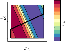
In many applications, like image analysis, $D$ can be in the order of thousands or millions. But even $D=10$ is a high dimensionality for common Gaussian process models, not only from a computational, but also from an informational, perspective. Because standard gp covariance functions stipulate that function values separated by more than a few input length scales are negligibly correlated, for high $D$, almost all of $\mathcal{X}$ is uncorrelated with observed data. Hence data is effectively ignored during most predictions, and learning is impossible. Practical experience shows, however, that many functions are insensitive to some of their inputs (Wang et al., 2013), thus have low effective dimensionality (Figure 1). Our goal is to discover a $R\in\mathbb{R}^{d\times D}$ such that, for low-dimensional $\mathcal{U}\subset\mathbb{R}^{d}$, $u=xR^{\intercal},\ \forall u\in\mathcal{U},\ x\in\mathcal{X}$ and $f(x)=\tilde{f}(u)$ for a new function, $\tilde{f}\colon\mathcal{U}\to\mathbb{R}$. The discussion here will be restricted to pre-defined $d$: in reality, this is likely to be defined as the maximum number of dimensions that can be feasibly considered in light of computational constraints. If the actual $d$ is lower than this limit, $R$ can be padded with rows of zeros.

Figure 1: A function $f$ with a one dimensional linear embedding (searching over the thick black lines captures all variation of the function) and its box-bounded domain $\mathcal{X}$. Our aim is to learn this embedding, represented by embedding matrix $R\in\mathbb{R}^{1\times 2}$, by selecting evaluations of $f$ in some search space.

We adopt a gp prior on $\tilde{f}$ with mean and covariance functions $\tilde{\mu}$ and $\tilde{\kappa}$, respectively. The linear embedding induces another gp prior $p(f)=\mathcal{GP}(f;\mu,\kappa)$, where $\mu(x)=\tilde{\mu}(x\,R^{\intercal})$ and $\kappa(x,x^{\prime})=\tilde{\kappa}(x\,R^{\intercal},x^{\prime}\,R^{\intercal})$. For example, if $\tilde{\kappa}$ is the well-known isotropic exponentiated-quadratic (squared-exponential, radial basis function, Gaussian) covariance, $\tilde{\kappa}(u,u^{\prime}):=\gamma^{2}\exp\left[-\frac{1}{2}(u-u^{\prime})(u-u^{\prime})^{\intercal}\right]$ with output scale $\gamma$, $\kappa$ on $f$ is the Mahalanobis exponentiated-quadratic covariance

$$\kappa(x,x^{\prime})=\gamma^{2}\exp\left[-\frac{1}{2}(x-x^{\prime})R^{\intercal}R(x-x^{\prime})^{\intercal}\right].$$ (1)

If $d=D=1$, then $R\in\mathbb{R}$ is an inverse length scale. We will return to this one-dimensional example later to build intuition. A further special case is a diagonal $R$ (assuming $d=D$), in which case $\kappa$ is the automatic relevance determination (ard) covariance (Neal, 1995), widely used to identify the most important inputs.

Given an appropriate $R$ with acceptably small $d$, learning about $f$ is possible even for large $D$, because the regression problem is reduced to the manageable space $\mathbb{R}^{d}$. This can remain true even in the case of an uncertain $R$: in particular, assume a prior $p(R)=\mathcal{N}(R;\hat{R},\Sigma)$. Thus, recalling that $u=xR^{\intercal}$, and using standard Gaussian identities, if $d=1$, $p(u\mid x)=\mathcal{N}(u;x\hat{R}^{\intercal},x\Sigma x^{\intercal})$. If $d>1$, $\Sigma$ is $\text{Cov}[\text{vect}(R)]$, resulting in another Gaussian for $p(u\mid x)$ that is only slightly more involved than in the $d=1$ case. As such, regression on $f$ reduces to gp regression on $\tilde{f}$, whose domain is the much smaller $\mathcal{U}\subset\mathbb{R}^{d}$, but with uncertain, Gaussian-distributed, inputs. Unlike the work of McHutchon & Rasmussen (2011), giving an existing approach to gp regression with uncertain inputs, the Gaussian over the inputs here is correlated; the location of a datum is correlated with all others via mutual dependence on $R$. And unlike the setting considered by Girard & Murray-Smith (2005), there is no natural ordering of this domain enabling an iterative procedure. The following section describes a novel means of regression with uncertain embedding $R$.

2.1 Approximating the posterior on $R$

The log-likelihood of $R$, after $N$ observations forming a dataset $\mathcal{D}:=({Y},X)\in\mathbb{R}^{N}\times\mathbb{R}^{N\times D}$, is

$$\log p(Y\mid X,R) =\log\mathcal{N}(Y;\mu_{X},K_{XX}+\sigma^{2}\mathbb{I})$$ (2)

$$=-\frac{1}{2}\big{[}(Y-\mu_{X})^{\intercal}(K_{XX}+\sigma^{2}\mathbb{I})^{-1}({Y}-\mu_{X})$$

$$\quad+\log\lvert K_{XX}+\sigma^{2}\mathbb{I}\rvert+N\log 2\pi\big{]}.$$

As $\mu_{X}:=\mu(X)$ and $K_{XX}:=\kappa(X,X)$ have non-linear dependence upon $R$, so does $p(Y\mid X,R)$. Even a simplistic prior on the elements of $R$ thus gives a complicated posterior. We will use a Laplace approximation for $p(R\mid\mathcal{D})$ to attain a tractable algorithm. To construct a Gaussian approximation, $\mathcal{N}(R;\hat{R},\Sigma)\simeq p(R\mid\mathcal{D})$, we find a mode of the posterior of $p(R\mid\mathcal{D})$ and set this mode as the mean $\hat{R}$ of our approximate distribution. The covariance of the Gaussian approximation is taken as the inverse Hessian of the negative logarithm of the posterior evaluated at $\hat{R}$,

$$\Sigma^{-1}=-\nabla\nabla^{\intercal}\log p(R\mid\mathcal{D})\bigr{\rvert}_{R=\hat{R}}.$$ (3)

2.1.1 Computational Cost

How costly is it to construct the Laplace approximation of Equation (3)? Since $D$ may be a large number, active learning should have low cost in $D$. This section shows that the required computations can be performed in time linear in $D$, using standard approximate numerical methods. It is a technical aspect that readers not interested in details may want to skip over.

Up to normalization, the log posterior is the sum of log prior and log likelihood (2). The former can be chosen very simplistically; the latter has gradient and Hessian given by, defining $G:=\kappa_{XX}+\sigma^{2}\mathbb{I}$ and $\Gamma:=G^{-1}({Y}-\mu_{X})$,

$$-2\frac{\partial\log p({Y}\mid X,R)}{\partial\theta} =-\Gamma^{\intercal}\frac{\partial\kappa_{XX}}{\partial\theta}\Gamma+\operatorname{Tr}\left[G^{-1}\frac{\partial\kappa_{XX}}{\partial\theta}\right];$$

$$-2\frac{\partial^{2}\log p({Y}\mid X,R)}{\partial\theta\partial\eta} =2\Gamma^{\intercal}\frac{\partial\kappa_{XX}}{\partial\eta}G^{-1}\frac{\partial\kappa_{XX}}{\partial\theta}\Gamma$$ (4)

$$-\operatorname{Tr}\left[G^{-1}\frac{\partial\kappa_{XX}}{\partial\eta}G^{-1}\frac{\partial\kappa_{XX}}{\partial\theta}\right]$$

$$-\Gamma^{\intercal}\frac{\partial^{2}\kappa_{XX}}{\partial\theta\partial\eta}\Gamma+\operatorname{Tr}\left[G^{-1}\frac{\partial^{2}\kappa_{XX}}{\partial\theta\partial\eta}\right].$$

Together with the analogous expressions for a prior $p(R)$, these expressions can be used to find a maximum of the posterior distribution (e.g., via a quasi-Newton method), and the Hessian matrix required for the Laplace approximation to $p(R\mid\mathcal{D})$. The computational cost of evaluating these expressions depends on the precise algebraic form of the kernel $\kappa$.

For the exponentiated quadratic kernel of Equation 1, careful analysis shows that the storage cost for the Hessian of (2) is $\mathcal{O}(N^{2}dD)$, and its structure allows its multiplication with a vector in $\mathcal{O}(N^{2}dD)$. The corresponding derivations are tedious and not particularly enlightening. To give an intuition, consider the most involved term in (4): Using the short-hand $\Delta^{ij}_{\ell}:=x_{i\ell}-x_{j\ell}$, a straightforward derivation gives the form

$$H^{1}_{k\ell,ab}: =-\sum_{ij}\Gamma_{i}\frac{\partial^{2}\kappa(x_{i},x_{j})}{\partial R_{k\ell}\partial R_{ab}}\Gamma_{j}$$

$$=\sum_{ijop}R_{ko}\Delta^{ij}_{o}\Delta^{ij}_{\ell}\Gamma_{i}\kappa(x_{i},x_{j})\Gamma_{j}R_{ap}\Delta^{ij}_{p}\Delta_{b}^{ij}$$

$$\quad-\sum_{ij}\delta_{ka}\Delta^{ij}_{b}\Gamma_{i}\kappa(x_{i},x_{j})\Gamma_{j}\Delta_{\ell}^{ij}.$$

Multiplication of this term with some vector $g_{ab}$ (resulting from stacking the elements of the $D\times d$ matrix $g$ into a vector) requires storage of the $d\times N\times N$ array $R\Delta$ with elements $(R\Delta)^{ij}_{k}$, the $D\times N\times N$ array $\Delta$ with elements $\Delta_{\ell}^{ij}$, and the $N\times N$ matrix $\Gamma\Gamma^{\intercal}\otimes K$. Multiplication then takes the form

$$[H^{1}g]_{k\ell} =\sum_{j=1}^{N}\sum_{i=1}^{N}(R\Delta)_{k}^{ij}\Delta_{\ell}^{ij}\Gamma_{i}\Gamma_{j}\kappa_{x_{i}x_{j}}$$ (5)

$$\quad\cdot\underbrace{\left[\sum_{a=1}^{d}(R\Delta)^{ij}_{a}\left[\sum_{b=1}^{D}\Delta_{b}^{ij}g_{ab}\right]\right]}_{\text{compute once in $\mathcal{O}(N^{2}dD)$, store in $\mathcal{O}(N^{2})$.}}$$

Since the $N\times N$ matrix in the square brackets is independent of $k\ell$, it can be re-used in the $dD$ computations required to evaluate the full matrix-vector product, so the overall computation cost of this product is $\mathcal{O}(N^{2}dD)$. The other required terms are of similar form. This means that approximate inversion of the Hessian, using an iterative solver like the Lanczos or conjugate gradient methods, is achievable in time linear in $D$. The methods described here are computationally feasible even for high-dimensional problems. Our implementation of the active method, which will be released along with this text, does not yet allow this kind of scalability, but the derivations above show that it is feasible in principle.

3 Approximate marginalization of Gaussian process hyperparameters

To turn the approximate Gaussian belief on $R$ into an approximate Gaussian process belief on $f$, the active learning algorithm (constructed in Section 4) requires an (approximate) means of integrating over the belief on $R$. The elements of $R$ form hyperparameters of the gp model. The problem of dealing with uncertainty in Gaussian process hyperparameters is a general one, also faced by other, non-active, Gaussian process regression models. This section presents a novel means of approximately integrating over the hyperparameters of a gp. The most widely used approach to learning gp hyperparameters is type-II maximum likelihood estimation (evidence maximization), or maximum a-posteriori (map) estimation, which both approximate the likelihood as a delta function. However, ignoring the uncertainty in the hyperparameters in this way can lead to pathologies (MacKay, 2003).

For compact notation, all hyperparameters to be marginalized will be subsumed into a vector $\theta$. We will denote as $m_{f|\mathcal{D},\theta}(x)$ the gp posterior mean prediction for $f(x)$ conditioned on data $\mathcal{D}$ and $\theta$, and similarly as $V_{f|\mathcal{D},\theta}(x)$ the posterior variance $V$ of $f(x)$ conditioned on $\mathcal{D}$ and $\theta$.

We seek an approximation to the intractable posterior for $f_{\ast}=f(x_{\ast})$, which requires marginalization over $\theta$,

$$p(f_{\ast}\mid\mathcal{D})=\int p(f_{\ast}\mid\mathcal{D},\theta)\,p(\theta\mid\mathcal{D})\,\mathrm{d}\theta.$$ (6)

Assume a Gaussian conditional, $p\!\left(\theta\middle|\mathcal{D}\right)=\mathcal{N}(\theta;\hat{\theta},\Sigma)$ on the hyperparameters, such as the approximate distribution over $R$ constructed in the preceding section. To make the integral in (6) tractable, we seek a linear approximation

$$p\!\left(f_{\ast}\middle|\mathcal{D},\theta\right) =\mathcal{N}\bigl{(}f_{\ast};m_{f\mid\mathcal{D},\theta}(x_{\ast}),V_{f\mid\mathcal{D},\theta}(x_{\ast})\bigr{)}$$ (7)

$$\simeq q(f_{\ast};\theta):=\mathcal{N}(f_{\ast};a^{\intercal}\theta+b,\nu^{2}),$$ (8)

using free parameters $a,b,\nu^{2}$ to optimize the fit. The motivation for this approximation is that it yields a tractable marginal, $p\!\left(f_{\ast}\middle|\mathcal{D}\right)\simeq\mathcal{N}(f_{\ast};a^{\intercal}\hat{\theta}+b,\nu^{2}+a^{\intercal}\Sigma a)$. Further, the posterior for $\theta$ typically has quite narrow width, over which $p\!\left(f_{\ast}\middle|\mathcal{D},\theta\right)$’s dependence on $\theta$ can be reasonably approximated. We choose the variables $a,b,\nu^{2}$ by matching a local expansion of $q(f_{*}\mid\theta)$ to $p\!\left(f_{\ast}\middle|\mathcal{D},\theta\right)$. The expansion will be performed at $\theta=\hat{\theta}$, and at a $f_{\star}=\hat{f}_{\star}$ to be determined. Specifically, we match as

$$\left.\frac{\partial}{\partial f_{\ast}}q(f_{\ast};\theta)\right\mid_{\hat{\theta},\hat{f}_{\star}} =\left.\frac{\partial}{\partial f_{\ast}}p\!\left(f_{\ast}\middle|\mathcal{D},\theta\right)\right\mid_{\hat{\theta},\hat{f}_{\star}},$$ (9)

$$\left.\frac{\partial}{\partial\theta_{i}}q(f_{\ast};\theta)\right\mid_{\hat{\theta},\hat{f}_{\star}} =\left.\frac{\partial}{\partial\theta_{i}}p\!\left(f_{\ast}\middle|\mathcal{D},\theta\right)\right\mid_{\hat{\theta},\hat{f}_{\star}},$$ (10)

$$\left.\frac{\partial^{2}}{\partial f_{\ast}^{2}}q(f_{\ast};\theta)\right\mid_{\hat{\theta},\hat{f}_{\star}} =\left.\frac{\partial^{2}}{\partial f_{\ast}^{2}}p\!\left(f_{\ast}\middle|\mathcal{D},\theta\right)\right\mid_{\hat{\theta},\hat{f}_{\star}},$$ (11)

$$\left.\frac{\partial^{2}}{\partial f_{\ast}\partial\theta_{i}}q(f_{\ast};\theta)\right\mid_{\hat{\theta},\hat{f}_{\star}} =\left.\frac{\partial^{2}}{\partial f_{\ast}\partial\theta_{i}}p\!\left(f_{\ast}\middle|\mathcal{D},\theta\right)\right\mid_{\hat{\theta},\hat{f}_{\star}}\,.$$ (12)

An alternative set of constraints could be constructed by including second derivatives with respect to $\theta$. But this would require computation scaling as $O((\#\theta)^{2})$, prohibitive for large numbers of hyperparameters, such as the $D\times d$ required to parameterize $R$ for large $D$. We define

$$\hat{m}:=m_{f|\mathcal{D},\hat{\theta}}\quad\text{and}\quad\frac{\partial\hat{m}}{\partial\theta_{i}}:=\frac{\partial m_{f|\mathcal{D},\theta}}{\partial\theta_{i}}\big{|}_{\theta=\hat{\theta}},$$ (13)

along with analogous expressions for $\hat{V}$ and $\frac{\partial\hat{V}}{\partial\theta_{i}}$. Turning to solving for $a,b,\nu^{2}$ and $f_{\star}$, note that, firstly, (9) implies that $a^{\intercal}\hat{\theta}+b=\hat{m}$, and that (11) implies that $\nu^{2}=\hat{V}$. Rearranging (10) and (12), respectively, we have

$$2a_{i} =\frac{\partial\hat{V}}{\partial\theta_{i}}\Biggl{(}\frac{1}{\hat{f}_{\star}-\hat{m}}-\frac{\hat{f}_{\star}-\hat{m}}{\hat{V}}\Biggr{)}+2\frac{\partial\hat{m}}{\partial\theta_{i}}\,,$$ (14)

$$2a_{i} =2\frac{\partial\hat{V}}{\partial\theta_{i}}\frac{\hat{f}_{\star}-\hat{m}}{\hat{V}}+2\frac{\partial\hat{m}}{\partial\theta_{i}}\,.$$ (15)

(14) and (15) can be solved only for

$$a_{i} =a_{i\pm}:=\pm\frac{1}{\sqrt{3\hat{V}}}\frac{\partial\hat{V}}{\partial\theta_{i}}+\frac{\partial\hat{m}}{\partial\theta_{i}}$$ (16)

$$f_{\ast} =\hat{f}_{\ast\pm}:=\hat{m}(x_{\ast})\pm\sqrt{\frac{\hat{V}(x_{\ast})}{3}}.$$ (17)

In particular, note that the intuitive choice $f_{\ast}=\hat{m}(x_{\ast})$, for which $\frac{\partial}{\partial f_{\ast}}p\!\left(f_{\ast}\middle|\mathcal{D},\theta\right)=0$, gives $q$ inconsistent constraints related to its variation with $\theta$. Introducing the separation of $\surd(\nicefrac{{\hat{V}(x_{\ast})}}{{3}})$ provides optimal information about the curvature of $p\!\left(f_{\ast}\middle|\mathcal{D},\theta\right)$ with $\theta$. Hence there are two possible values, $\hat{f}_{\ast\pm}$, to expand around, giving a separate Gaussian approximation for each. We average over the two solutions, giving an approximation that is a mixture of two Gaussians. We then further approximate this as a single moment-matched Gaussian.

The consequence of this approximation is that

$$p(f_{\ast}\mid\mathcal{D})\simeq\mathcal{N}\bigl{(}f_{\ast};\tilde{m}_{f|\mathcal{D}}(x_{\ast}),\tilde{V}_{f|\mathcal{D}}(x_{\ast})\bigr{)},$$ (18)

where the marginal mean for $f_{\ast}$ is $\tilde{m}_{f|\mathcal{D}}(x_{\ast}):=\hat{m}(x_{\ast})$, and the marginal variance is

$$\tilde{V}_{f|\mathcal{D}}(x_{\ast}) :=\frac{4}{3}\hat{V}(x_{\ast})+\frac{\partial\hat{m}(x_{\ast})}{\partial\theta}^{\intercal}\Sigma\,\frac{\partial\hat{m}(x_{\ast})}{\partial\theta}$$

$$\quad+\frac{1}{3\hat{V}(x_{\ast})}\frac{\partial\hat{V}(x_{\ast})}{\partial\theta}^{\intercal}\Sigma\,\frac{\partial\hat{V}(x_{\ast})}{\partial\theta}\,.$$ (19)

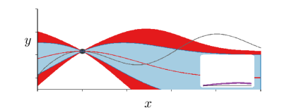
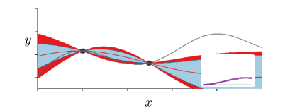
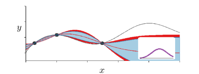
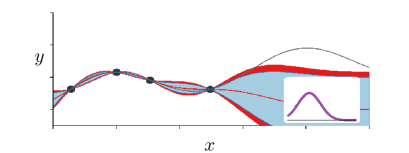
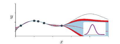
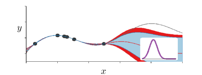
Figure 2 provides an illustration of our approximate marginal gp (henceforth abbreviated as mgp).

Our approach is similar to that of Osborne et al. (2012) (bbq), for which $\tilde{V}_{f|\mathcal{D}}=V_{f|\mathcal{D},\hat{\theta}}+\frac{\partial\hat{m}}{\partial\theta}^{\intercal}\Sigma\frac{\partial\hat{m}}{\partial\theta}$. However, bbq ignores the variation of the predictive variance with changes in hyperparameters.

To compare the two methods, we generated (from a gp) $10\times D$ random function values, $\mathcal{D}$, where $D$ is the problem dimension. We then trained a gp with zero prior mean and ard covariance on that data, and performed prediction for $10\times D$ test data. Test points, $(x_{\ast},y_{\ast})$, were generated a small number (drawn from $\mathcal{U}(1,3)$) of input scales away from a training point in a uniformly random direction. The mgp and bbq were used to approximately marginalize over all gp hyperparameters (the output scale and $D$ input scales), computing posteriors for the test points. We considered $D\in\{5,10,20\}$ and calculated the mean skld over fifty random repetitions of each experiment. We additionally tested on two real datasets: yacht hydrodynamics (Gerritsma et al., 1981) and (centered) concrete compressive strength (Yeh, 1998). In these two, a random selection of 50 and 100 points, respectively, was used for training and the remainder for testing. All else was as above, with the exception that ten random partitions of each dataset were considered.

We evaluate performance using the symmetrized Kullback–Leibler divergence (skld) between approximate posteriors and the “true” posterior (obtained using a run of slice sampling (Neal, 2003) with $10^{5}$ samples and $10^{4}$ burn-in); the better the approximate marginalization, the smaller this divergence. We additionally measured the average negative predictive log-likelihood, $-\mathbb{E}\bigl{[}\log p(y_{\ast}\mid x_{\ast},\mathcal{D})\bigr{]}$, on the test points $(x_{\ast},y_{\ast})$. Results are displayed in Table 1; it can be seen that the mgp provides both superior predictive likelihoods and posteriors closer to the “true” distributions. The only exception is found on the yacht dataset, where the mgp’s skld score was penalized for having predictive variances that were consistently slightly larger than the “true” variances. However, these conservative variances, in better accommodating test points that were unexpectedly large or small, led to better likelihoods than the consistently over-confident map and bbq predictions.

Figure 2: Approximate marginalization (mgp) of covariance hyperparameters $\theta$ increases the predictive variance to closely match the “true” posterior (obtained using slice sampling with $10^{5}$ samples). bbq (Osborne et al., 2012) provides a standard deviation differing from the map standard deviation by less than 3.1% everywhere, and would hence be largely invisible on this plot. The bottom of the figure displays the (normalized) mutual information $I\bigl{(}\Theta;F(x)\bigr{)}$ (equal to the bald utility function $\upsilon(x)$) for the various methods, and their maxima, giving the optimal positions for the next function evaluations. The mgp position is very close to the true position.

Table 1: Mean negative log-likelihood for test points and mean skld (nats) between approximate and true posteriors. Both metrics were averaged over test points, as well as over fifty and ten random repeats for synthetic and real experiments, respectively.

		$-\mathbb{E}\bigl{[}\log p(y_{\ast}\mid x_{\ast},\mathcal{D})\bigr{]}$			skld
problem	dim	map	bbq	mgp	map	bbq	mgp
synthetic	5	$3.58$	$2.67$	${\bf 1}.{\bf 73}$	$0.216$	$0.144$	${\bf 0}.{\bf 0835}$
synthetic	10	$3.57$	$3.10$	${\bf 1}.{\bf 86}$	$0.872$	$0.758$	${\bf 0}.{\bf 465}$
synthetic	20	$1.46$	$1.41$	${\bf 0}.{\bf 782}$	$1.01$	$0.947$	${\bf 0}.{\bf 500}$
yacht	6	$123.0$	$97.8$	${\bf 56}.{\bf 8}$	$0.0322$	${\bf 0}.{\bf 0133}$	$0.0323$
concrete	8	$2.96\cdot 10^{9}$	$2.96\cdot 10^{9}$	${\bf 1}.{\mathbf{67\cdot 10^{9}}}$	$0.413$	$0.347$	${\bf 0}.{\bf 337}$

4 Active learning of Gaussian process hyperparameters

Now we turn to the question of actively selecting observation locations to hasten our learning of $R$. We employ an active learning strategy due to Houlsby et al. (2011), known as Bayesian active learning by disagreement (bald). The idea is that, in selecting the location $x$ of a function evaluation $f$ to learn parameters $\theta$, a sensible utility function is the expected reduction in the entropy of $\theta$,

$$\upsilon(x):=H(\Theta)-H(\Theta\mid F)=H(F)-H(F\mid\Theta),$$ (20)

also equal to the mutual information $I(\Theta;F)$ between $f$ and $\theta$. Mutual information, unlike differential entropies, is well-defined: the bald objective is insensitive to changes in the representation of $f$ and $\theta$. The right-hand-side of (20), the expected reduction in the entropy of $f$ given the provision of $\theta$, is particularly interesting. For our purposes, $\theta$ will parameterize $R\in\mathbb{R}^{d\times D}$: that is, $\theta$ is very high-dimensional, making the computation of $H(\Theta)$ computationally demanding. In contrast, the calculation of the entropy of $f\in\mathbb{R}$ is usually easy or even trivial. The right-hand side of (20) is particularly straightforward to evaluate under the approximation of Section 3, for which $p(f\mid\mathcal{D},\theta)$ and the marginal $p(f\mid\mathcal{D})$ are both Gaussian. Further, under this approximation, $p(f\mid\mathcal{D},\theta)$ has variance $\nu^{2}=\hat{V}$ that is independent of $\theta$, hence, $H(F\mid\Theta)=H(F\mid\Theta=\hat{\theta})$. We henceforth consider the equivalent but transformed utility function

$$\upsilon^{\prime}(x)=\tilde{V}_{f|\mathcal{D}}(x)\,\Big{(}V_{f|\mathcal{D},\hat{\theta}}(x)\Big{)}^{-1}.$$ (21)

The mgp approximation has only a slight influence on this objective – Figure 2 compares it to a full mcmc-derived marginal. With reference to (19), (21) encourages evaluations where the posterior mean and covariance functions are most sensitive to changes in $\theta$ (Figure 3), normalized by the variance in $f$: such points are most informative about the hyperparameters.

Figure 3: Active learning of the length scale of a one-dimensional gp (beginning at the top left and continuing across and then down): the next sample is taken where the map and approximate variances maximally disagree, normalized by the map variance. Samples are taken at a variety of separations to refine belief about the length scale. The inset plots (all of which share axes) display the approximate posteriors over log-length scales, which tighten with increasing numbers of samples. The legend is identical to that of Figure 2.

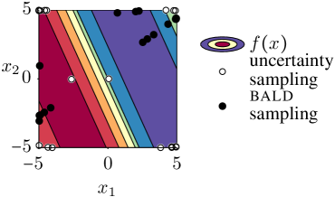
An alternative to bald is found in uncertainty sampling. Uncertainty sampling selects the location with highest variance, that is, its objective is simply $H(F)$, the first term in the bald objective. This considers only the variance of a single point, whereas the bald objective rewards points that assist in the learning of embeddings, thereby reducing the variance associated with all points. An empirical comparison of our method against uncertainty sampling follows below.

4.1 Active learning of linear embeddings for Gaussian processes

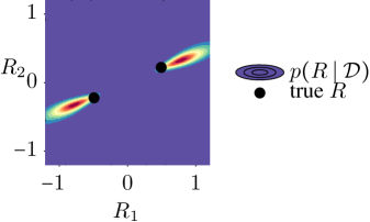
To apply bald to learning the linear embedding of a Gaussian process, we consider the case $R\subset\theta$; the gp hyperparameters define the embedding described in Section 2. Figure 4 demonstrates an example of active learning for the embedding of a two-dimensional function.

Figure 4: Left: Twenty samples selected by uncertainty sampling and bald for a function $f$ with a one dimensional linear embedding. Note that uncertainty sampling prefers corner locations, to maximize the variance in $u$, $x\Sigma x^{\intercal}$, and hence the variance in $f$; these points are less useful for learning $f$ and its embedding than those selected by bald. Right: the posterior over embeddings returned by the bald samples, concentrated near the true embedding (equivalent under negation).

The latent model of lower dimension renders optimizing an objective with domain $\mathcal{X}$ (e.g., $f(x)$, or the bald objective) feasible even for high dimensional $\mathcal{X}$. Instead of direct search over $\mathcal{X}$, one can choose a $u\in\mathcal{U}$, requiring search over only the low-dimensional $\mathcal{U}$, and then evaluate the objective at an $x\in\mathcal{X}$ for which $u=x\,R^{\intercal}$. A natural choice is the $x$ which is most likely to actually map to $u$ under $R$, that is, the $x$ for which $p(u\mid x)$ is as tight as possible. For example, we could minimize $\log\det\operatorname{cov}[u\mid x]$, subject to $\mathbb{E}[u\mid x]=x\,\hat{R}^{\intercal}$, by solving the appropriate program. For $d=1$, this is a quadratic program that minimizes the variance $x\Sigma x^{\intercal}$ under the equality constraint. Finally, we evaluate the objective at the solution.

For simplicity, we will henceforth assume $\mathcal{X}=[-1,1]^{D}$. For any box-bounded problem, there is an invertible affine transformation mapping the box to this $\mathcal{X}$; this then requires only that $R$ is composed with this transformation. Further, define the signature of the $i$th row of $R$ to be $[\text{sign}(R_{i1}),\text{sign}(R_{i2}),\ldots]$. Then, for the $i$th coordinate, the maximum and minimum value obtained by mapping the corners of $\mathcal{X}$ through $R$ are achieved by the corner matching this signature and its negative. This procedure defines the extreme corners of the search volume $\mathcal{U}$.

Consider the typical case in which we take $\tilde{\mu}$ as constant and $\tilde{\kappa}$ as isotropic (e.g., the exponentiated quadratic (1)). Since $p(f\mid X,R)$ is then invariant to orthogonal transformations of $R$ in $\mathbb{R}^{d}$, there is no unique embedding. In the special case $d=1$, $R$ and $-R$ are equivalent. For most means and covariances there will be similar symmetries, and likely ever more of them as $d$ increases. We therefore evaluate the performance of our algorithms not by comparing estimated to true $R$s, which is difficult due to these symmetries, but rather in the direct predictive performance for $f$.

4.2 Active learning of linear embeddings experiments

We now present the results of applying our proposed method for learning linear embeddings on both real and synthetic data with dimension up to $D=318$. Given a function $f\colon\mathcal{X}\to\mathbb{R}$ with a known or suspected low-dimensional embedding, we compare the following methods for sequentially selecting $N=100$ observations from the domain $[-1,1]^{D}$: random sampling (rand), a Latin hypercube design (lh), uncertainty sampling (unc), and bald. unc and bald use identical models (Laplace approximation on $R$ followed by mgp) and hyperparameter priors. We also compare with lasso, choosing the regularization parameter by minimizing squared loss on the training data. The functions that these methods are compared on are:

• Synthetic in-model data drawn from a gp matching our model with an embedding drawn from our prior, for $d\in\{2,3\}$ and $D\in\{10,20\}$.

• The Branin function, a popular test function for global optimization ($d=2$), embedded in $D\in\{10,20\}$ via an embedding drawn from our prior.

• The temperature data described in Snelson & Ghahramani (2006) ($D=106$), with $d=2$. The associated prediction problem concerns future temperature at a weather station, given the output of a circulation model. The training and validation points were combined to form the dataset, comprising 10 675 points.

• The normalized “communities and crime” (c&c) dataset from the uci Machine Learning Repository ($D=96$), with $d=2$. The task here is to predict the number of violent crimes per capita in a set of us communities given historical data from the us Census and fbi. The lemas survey features were discarded due to missing values, as was a single record missing the “AsianPerCap” attribute, leaving $1\,993$ points.

• The “relative location of ct slices on axial axis” dataset from the uci Machine Learning Repository ($D=318$), with $d=2$. The task is to use features extracted from slices of a ct scan to predict its vertical location in the human body. Missing features were replaced with zeros. Only axial locations in the range $[50,60]$ were used. Features that did not vary over these points were discarded, leaving $3\,071$ points.

The ct slices and communities and crime datasets are, respectively, the highest- and third-highest-dimensional regression datasets available in the uci Machine Learning Repository with real attributes; in second place is an unnormalized version of the c&c dataset.

Table 2: The combination of mgp and bald actively learns embeddings whose predictive performance improves on alternatives. Average negative log predictive probability and average rmse on test functions for various $D$ and $d$.

		$-\mathbb{E}\bigl{[}\log p(y_{\ast}\mid x_{\ast},\hat{R})\bigr{]}$					rmse
dataset	$D$/	$d$	rand	lh	unc	bald	rand	lh	unc	bald	lasso
synthetic	10/	2	$0.272$	$0.224$	$-0.564$	${\bf-0}.{\bf 649}$	$0.412$	$0.371$	$0.146$	${\bf 0}.{\bf 138}$	$0.842$
synthetic	10/	3	$0.711$	$0.999$	$0.662$	${\bf 0}.{\bf 465}$	$0.553$	$0.687$	$0.557$	${\bf 0}.{\bf 523}$	$0.864$
synthetic	20/	2	$0.804$	$0.745$	$0.749$	${\bf 0}.{\bf 470}$	$0.578$	$0.549$	$0.551$	${\bf 0}.{\bf 464}$	$0.853$
synthetic	20/	3	$1.07$	$1.10$	$1.04$	${\bf 0}.{\bf 888}$	$0.714$	$0.740$	$0.700$	${\bf 0}.{\bf 617}$	$0.883$
Branin	10/	2	$3.87$	$3.90$	$1.58$	${\bf 0}.{\bf 0165}$	$18.2$	$17.8$	$3.63$	${\bf 2}.{\bf 29}$	$40.0$
Branin	20/	2	$4.00$	$3.70$	${\bf 3}.{\bf 55}$	$3.63$	$18.3$	$14.8$	${\bf 13}.{\bf 4}$	$15.0$	$39.1$
communities & crime	96/	2	$1.09$	—	$1.17$	${\bf 1}.{\bf 01}$	$0.720$	—	$0.782$	${\bf 0}.{\bf 661}$	$1.16$
temperature	106/	2	$0.566$	—	$0.583$	${\bf 0}.{\bf 318}$	$0.423$	—	$0.427$	${\bf 0}.{\bf 328}$	$0.430$
ct slices	318/	2	$1.30$	—	$1.26$	${\bf 1}.{\bf 16}$	$0.878$	—	$0.845$	${\bf 0}.{\bf 767}$	$0.900$

For the synthetic and Branin problems, where the true embedding $R$ was chosen explicitly, we report averages over five separate experiments differing only in the choice of $R$. On these datasets, the unc and bald methods selected points by successively maximizing their respective objectives on a set of $20\,000$ fixed points in the input domain, $10\,000$ selected uniformly in $[-1,1]^{D}$ and $10\,000$ selected uniformly in the unit $D$-sphere. For a given $D$, these points were fixed across methods and experimental runs. This choice allows us to compare methods based only on their objectives and not the means of optimizing them.

For the real datasets (temperature, communities and crimes, and ct slices), each method selected from the available points; lh is incapable of doing so and so is not considered on these datasets. The real datasets were further processed by transforming all features to the box $[-1,1]^{D}$ via the “subtract min, divide by max” map and normalizing the outputs to have zero mean and unit variance. For the synthetic problems, we added i.i.d. Gaussian observation noise with variance $\sigma^{2}=(0.1)^{2}$. For the remaining problems, the datapoints were used directly (assuming that these real measurements already reflect noise).

After each method selected 100 observations, we compare the quality of the learned embeddings by fixing the hyperparameters of a gp to the map embedding at termination and measuring predictive performance. This is intended to emulate a fixed-budget embedding learning phase followed by an experiment using only the most likely $R$. We chose $N=100$ training points and $1\,000$ test points uniformly at random from those available; these points are common to all methods. We report root-mean-square-error and the average negative predictive log-likelihood on the test points. The rmse measures predictive accuracy, whereas the log-likelihood additionally captures the accuracy of variance estimates. This procedure was repeated 10 times for each experiment; the reported numbers are averages.

The embedding prior $p(R)$ was set to be i.i.d. zero-mean Gaussian with standard deviation $\nicefrac{{5}}{{4}}D^{-1}$. This choice roughly implies that we expect $[-1,1]^{D}$ to map approximately within $[-2.5,2.5]^{d}$, a box five length scales on each side, under the unknown embedding. This prior is extremely diffuse and does not encode any structure of $R$ beyond prefering low-magnitude values. At each step, the mode of the log posterior over $R$ was found using using l-bfgs, starting from both the previous best point and one random restart drawn from $p(R)$.

The results are displayed in Table 2. The active algorithm achieves the most accurate predictions on all but one problem, including each of the real datasets, according to both metrics. These results strongly suggest an advantage for actively learning linear embeddings.

5 Conclusions

Active learning in regression tasks should include hyperparameters, in addition to the function model itself. Here we studied simultaneous active learning of the function and a low-dimensional linear embedding of its input domain. We also developed a novel means of approximately integrating over the hyperparameters of a gp model. The resulting algorithm addresses needs in a number of domains, including Bayesian optimization, Bayesian quadrature, and also the underlying idea of nonparametric Gaussian regression itself. Empirical evaluation demonstrates the efficacy of the resulting algorithm on both synthetic and real problems in up to $318$ dimensions, and an analysis of computational cost shows that the algorithm can, at least in principle, be scaled to problems of much larger dimensionality as well.

References

- Bergstra & Bengio (2012) Bergstra, J. and Bengio, Y. Random search for hyper-parameter optimization. Journal of Machine Learning Research, 13:281–305, 2012.
- Brochu et al. (2010) Brochu, E., Cora, V. M., and de Freitas, N. A tutorial on Bayesian optimization of expensive cost functions, with application to active user modeling and hierarchical reinforcement learning. arXiv preprint arXiv:1012.2599, 2010.
- Candes & Tao (2007) Candes, E. and Tao, T. The Dantzig selector: Statistical estimation when is much larger than . Annals of Statistics, 35(6):2313–2351, 2007.
- Carpentier & Munos (2012) Carpentier, A. and Munos, R. Bandit theory meets compressed sensing for high dimensional stochastic linear bandit. arXiv preprint arXiv:1205.4094, 2012.
- Chen et al. (2012) Chen, B., Castro, R., and Krause, A. Joint optimization and variable selection of high-dimensional Gaussian processes. In Proceedings of the 29th Annual International Conference on Machine Learning, 2012.
- Gerritsma et al. (1981) Gerritsma, J., Onnink, R., and Versluis, A. Geometry, resistance and stability of the delft systematic yacht hull series. International Shipbuilding Progress, 28(328):276–297, 1981.
- Girard & Murray-Smith (2005) Girard, A. and Murray-Smith, R. Gaussian processes: Prediction at a noisy input and application to iterative multiple-step ahead forecasting of time-series. In Switching and Learning in Feedback Systems, number 3355 in Lecture Notes in Computer Science. Springer, 2005.
- Guestrin et al. (2005) Guestrin, C., Krause, A., and Singh, A. P. Near-optimal sensor placements in Gaussian processes. In Proceedings of the 22nd Annual International Conference on Machine Learning, pp. 265–272. ACM, 2005.
- Hennig & Kiefel (2012) Hennig, P. and Kiefel, M. Quasi-Newton methods – A new direction. In Proceedings of the 29th Annual International Conference on Machine Learning, 2012.
- Houlsby et al. (2011) Houlsby, N., Huszár, F., Ghahramani, Z., and Lengyel, M. Bayesian active learning for classification and preference learning. arXiv preprint arXiv:1112.5745, 2011.
- Hutter (2009) Hutter, F. Automated configuration of algorithms for solving hard computational problems. PhD thesis, University of British Columbia, 2009.
- Hutter et al. (2011) Hutter, F., Hoos, H., and Leyton-Brown, K. Sequential model-based optimization for general algorithm configuration. In Learning and Intelligent Optimization, pp. 507–523. Springer, 2011.
- Iwata et al. (2013) Iwata, T., Houlsby, N., and Ghahramani, Z. Active learning for interactive visualization. Proceedings of the 16th International Conference on Artificial Intelligence and Statistics (AISTATS 2013), (31), 2013.
- Lawrence (2012) Lawrence, N. D. A unifying probabilistic perspective for spectral dimensionality reduction: Insights and new models. Journal of Machine Learning Research, 13:1609–1638, 2012.
- MacKay (1992a) MacKay, D. J. C. Bayesian interpolation. Neural Computation, 4(3):415–447, 1992a.
- MacKay (1992b) MacKay, D. J. C. Information-based objective functions for active data selection. Neural Computation, 4(4):590–604, 1992b.
- MacKay (2003) MacKay, David J. C. Information theory, inference and learning algorithms. Cambridge University Press, 2003.
- McHutchon & Rasmussen (2011) McHutchon, A. and Rasmussen, C. E. Gaussian process training with input noise. In Advances in Neural Information Processing Systems 24, 2011.
- Neal (1995) Neal, R. M. Bayesian Learning for Neural Networks. PhD thesis, University of Toronto, 1995.
- Neal (2003) Neal, R. M. Slice sampling. Annals of Statistics, 31(3):705–767, 2003.
- O’Hagan (1991) O’Hagan, A. Bayes-Hermite quadrature. Journal of Statistical Planning and Inference, 29:245–260, 1991.
- Osborne et al. (2012) Osborne, M. A., Duvenaud, D., Garnett, R., Rasmussen, C. E., Roberts, S. J., and Ghahramani, Z. Active learning of model evidence using Bayesian quadrature. In Advances in Neural Information Processing Systems 25, pp. 46–54, 2012.
- Rasmussen & Williams (2006) Rasmussen, C. E. and Williams, C. K. I. Gaussian Processes for Machine Learning. MIT Press, 2006.
- Snelson & Ghahramani (2006) Snelson, E. and Ghahramani, Z. Variable noise and dimensionality reduction for sparse Gaussian processes. In Proceedings of the 22nd Conference on Uncertainty in Artificial Intelligence (UAI 2006), pp. 461–468, 2006.
- Tibshirani (1996) Tibshirani, R. Regression shrinkage and selection via the lasso. Journal of the Royal Statistical Society. Series B (Methodological), 58(1):267–288, 1996.
- Wang et al. (2013) Wang, Z., Zoghi, M., Hutter, F., Matheson, D., and de Freitas, N. Bayesian optimization in a billion dimensions via random embeddings. arXiv preprint arXiv:1301.1942, 2013.
- Williams & Rasmussen (1996) Williams, C. K. I. and Rasmussen, C. E. Gaussian processes for regression. In Advances in Neural Information Processing Systems 8, 1996.
- Yeh (1998) Yeh, I-C. Modeling of strength of high-performance concrete using artificial neural networks. Cement and Concrete Research, 28(12):1797–1808, 1998.