Cascading Failures in Networks with Proximate Dependent Nodes
Abstract
We study the mutual percolation of a system composed of two interdependent random regular networks. We introduce a notion of distance to explore the effects of the proximity of interdependent nodes on the cascade of failures after an initial attack. We find a non-trivial relation between the nature of the transition through which the networks disintegrate and the parameters of the system, which are the degree of the nodes and the maximum distance between interdependent nodes. We explain this relation by solving the problem analytically for the relevant set of cases.
Previous studies of the robustness of interdependent networks have
focused on networks in which there is no constraint on the distance
between the interdependent nodes
Huang ; Parshani ; Shao ; Buldyrev ; Hu ; Buldyrevnat ; Dong ; Gao ; Son . However, many dependency links in the
real world connect nearby nodes. For example, the international
network of seaports and the network of national highways form a
complex system. As seen recently from the effects of Hurricane
Sandy in New York City, if a seaport is damaged, the city that
depends on it will become isolated from the highway network due to the
lack of fuel. Similarly, a city without roads cannot supply a seaport properly. However, a city will depend on a nearby seaport, not
on one across the world. Li et. al Li investigated
distance-limited interdependent lattice networks by computer simulations and found that allowing only local interdependency links changed the resilience properties of the system. Here, we study the analytically tractable random networks.
We study the mutual percolation of two interdependent
random regular (RR) graphs. We build two identical networks, A and B,
each of whose nodes are labeled . Each node is randomly
connected by edges to exactly other nodes, in such a way that the two networks
have identical topologies. We then create one-to-one bidirectional dependency links, requiring that
the shortest path between the interdependent nodes does not exceed an
integer constant .
Formally, we establish two isomorphisms between
networks A and B, a topological isomorphism and a dependency
isomorphism. The topological isomorphism is defined for each node
as and . If and
are immediate neighbors in network A, then and are
immediate neighbors in network B and vice versa.
The dependency isomorphism has the property that if , then . We create a restriction that only if there are a maximum of
connectivity links on the shortest path connecting and
.
For simplicity, we introduce two more restrictions. We only set if there are no other possibilities for . Additionally, we require that if , then . This restriction decreases the computation time needed. Simulations suggest that the results for the models with and without the latter restriction are indistinguishable within the statistical error.
Following the mutual percolation model described in Buldyrev et
al. Buldyrevnat , we destroy a fraction of randomly
selected nodes in A. Any nodes that, as a result, lost their connectivity links to the largest cluster (as defined in classical, single-network percolation theory
newmanbook ; havlinbook ) are also destroyed. In the next stage, nodes in B that have their interdependent nodes in the other network destroyed are also destroyed. Consequently, the nodes that are isolated
from the largest cluster in B
as a result of the destruction of nodes in B are also destroyed. The iteration of this process, which alternates between the two networks, leads to a cascade of
failures. The cascade ends when no more nodes fail in either network. The pair of remaining largest interdependent clusters in both networks is called a largest mutual component. If in the thermodynamic limit
, the fraction of nodes in the largest mutual component is greater than zero, it is called the giant mutual component.
As
decreases, the giant component also decreases in size and eventually disappears at the value of that we call critical , or . We will denote for a
degree and distance as . We investigate how varies as
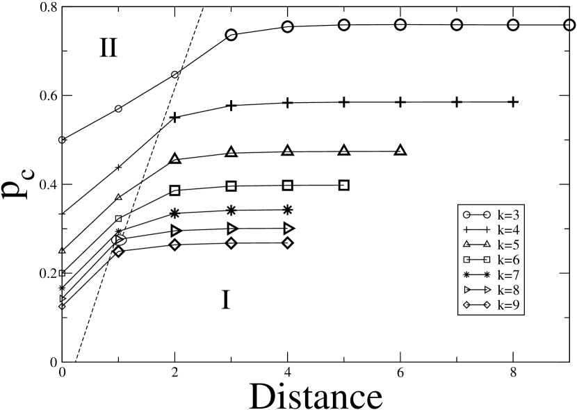
a function of and (Figure 1).

As the distance and the degree increase, the transition at shifts
from a second-order transition in which continuously approach zero to a first-order one, in which decreases discontinuously in the thermodynamic limit. The line separating these two regimes is shown in Fig. 1. Of particular note is the shift
for . If , the transition is second
order. For , the transition is first-order. For , we
observe two transitions: the first-order transition at followed by
the second-order transition at . As we will explain, the existence of the second-order transition in this case affects the behavior of the first-order transition.
For each value of , increases monotonically as increases. This monotonic increase is in contrast with the results
found by Li et al. Li , who found that in distance-limited
lattices, there is a maximum in as a function of . In Li et al.,
this maximum coincided with the distance at which the transition
shifts its nature from second-order for smaller distances to
first-order for larger distances. In our model, a similar shift occurs
at a very low value of and is not associated with a maximum of
.
If the transition is of the first-order,
the size of the largest mutual component of a finite network at a fixed value of may fluctuate dramatically. Due to
fluctuations always present in a finite system, can be close to the value , which is the fraction of nodes in the mutual giant component for at , where is a small positive number. In other cases, it can be close to , the value of at for . However, no values of are expected in the interval between and .
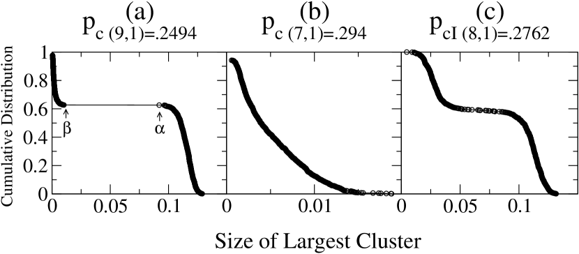
Fig. 2 (a) illustrates the first-order transition observed at ; we see that there is no
intermediate value of when the simulation is repeated for
many such systems. As the size of the network increases,
the distribution concentrates around and , with the probability density approaching a delta function at these two points. We define as the point where half of the realizations lead to each result. As the size of the network increases, goes to 0 in most cases. The sole exception is (Fig. 2 (c)).
In the case of second-
order transitions, the drop in is less dramatic. There is no
gap in the size distribution of the largest giant component (Fig. 2 (b)). Rather, there is a steady decline of the cumulative distribution of . Thus, and are not defined.
These two categories describe every transition with the exception of . There, we see a plateau in the cumulative
distribution of the largest component size, reminiscent of a first-order transition. However, there is no clear gap
in the distribution of the mutual giant
component in a finite network and we cannot clearly identify and (Fig. 2).

To explain the curious behavior of , as well as to better understand the general behavior of interdependent networks with distance constraints, we offer a brief synopsis of our analytic solution for the case where , which is the simplest case, in which we see the transition shift from second-order to first-order.
In our simulation, we establish dependency links in the following way:
At each step, we select at random a node that currently does not have a dependency link and set
two dependency links and , where is randomly chosen among ’s immediate neighbors without a dependency link, if at least one such neighbor exists. We call a dimer. If all of the neighbors of already have dependency links, we set and is called a monomer. In order to calculate , we find the fraction of indices that are monomers,
| (1) |
Finding the value of is a version of Rényi’s parking
problem Renyi that applies to a discrete graph.
We will present our full analytic solution of that problem and the derivation of Eq. (1) elsewhere.
In our analytic calculation of we will use the probability that a link leaving a dimer reaches a monomer. Because, in our algorithm, two monomers cannot be adjoining, any connectivity link that has a monomer at one end has a dimer at the other end. Thus, is simply
the number of links with monomers at one end divided by the number of
links that leave dimers, which is .
When , it is possible to express the problem of finding the mutual giant component of two networks as the problem of finding of a giant component in a single network, while taking into account the disruption caused by the other network. To determine for a single RR graph, percolation theory introduces a probability that a randomly selected link does not lead to the giant component. This probability satisfies the equation newmanbook
| (2) |
The first term on the right side of the equation refers to the probability that the link leads to a node that was destroyed in the initial attack, while the second term represents the probability that the node survived, but does not have any outgoing links that lead to the giant component.
Previous studies of interdependent networks
have used this equation Son , often modifying either the value
of Buldyrevnat ; Shao ; Parshani ; Hu or the degree
distribution Huang ; Dong ; Buldyrev . They use these modifications to describe the diminished network at each stage of the cascade. However, this method is only useful when the nodes destroyed in each stage of the cascade can be seen as a random subset of nodes in the other network. The distance restriction in our model precludes us from doing so. We modify the equation itself to account for the local
interdependency between our two networks. This allows us to study both networks at once and to account for more complex relationships between them.
When studying a link in network A, we assume that the link
starts from a node , such that its interdependent counterpart in network B, a priori belongs to the mutual giant component. This assumption allows us to isolate the effect that the destruction of nodes in network A will have. Formally, this is done by assuming that is artificially connected to the mutual giant component in a way that does not affect the topology in network A. We thus define as the probability that a randomly chosen link leaving node would not lead to the mutual giant component, if were to be artificially attached to the mutual giant component.
If the link leaving leads to a node that survived the initial
attack, represents the event that is not connected to the
mutual giant component via any of its outgoing links, even with our a priori assumption.
However, even if does not occur, may still be dead because its interdependent node
does not belong to the mutual giant component.
Accordingly, we define the event that the node is not
connected to the mutual giant component via links of network B.
Thus, we can write
| (3) |
where plays the role that did in Eq. (2). We need to study separately monomers, “matched” dimers (in which both nodes in the dimer survive the initial attack), and “unmatched” dimers, (in which only one of the two nodes survives). Eq. (3) is a general framework which must be adapted to account for the three different types of nodes in our system. We thus obtain three equations from Eq. (3). The equation for studies links that leave monomers, while the equation for studies links that leave matched dimers and the equation for studies links that leave unmatched dimers. We then calculate the probability that (the node to which the link leads) is a given type of node (for example, a monomer), and then multiply this by the probability that if is a monomer (for example), does not connects to the giant component, given our a priori assumption. Once we calculate these probabilities for each of the three types of nodes, we add these probabilities, finally arriving at the total probability that a node does not lead to the giant component, given our a priori assumption that its support node does. We find
| (4) | ||||||||
| (5) |
These two equations are relatively simple; is either just or . That is, , failure due to the second network, is either 1) impossible due to the a priori assumption, or 2) independent of . Case 1 occurs when both and are monomers or parts of matched dimers; in these cases, nodes that survived the initial attack connect and , allowing to be connected to the giant component. Case 2 occurs when is a part of an unmatched dimer; due to the local tree-like structure of the large RR network, the path that connects to its giant component will not overlap with the path that connects to its giant component. Thus, the existence of one path has no correlation with the existence of the other. The calculation of is more difficult. The events and are not always independent because ’s and ’s paths to the mutual giant component may overlap. We must find . Therefore, we introduce another two variables, and , which denote the probabilities that neither the link from to nor the link from to lead to the giant component. The principle in these cases is the same as the one used in the determination of and . can be expressed as a power of or . We find:
| (6) | ||||||
| (7) | ||||||
| (8) |
Finally, the fraction of nodes in the mutual giant component is
| (9) |
To solve the equations (Eqs. (4)-(8)), we define
, and a function , which represents the right hand sides of Eqs. (4)-(8). These
equations always have a trivial solution of , for which . Through an
iterative process ,
, we search for a
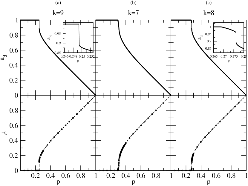
non-trivial fixed point for different values of . The results for are presented in
Figure 3. Our results for
coincide with our numerical data to within the precision of the simulation. We
remarkably see three types of transitions in the value of
as a function of , as the simulations indicated. For , we observe a
second-order transition. For , we find a first-order
transition. For , as decreases, we first see a first-order transition at
, where changes dramatically (but not to zero) and a second-order transition to when decreases to .

In conclusion, our results demonstrate the interesting behavior of collapsing random networks with distance-restricted dependency links.
We find that networks with long dependency distances,
are much more vulnerable than networks with short dependency distances.
Moreover, the networks with large dependency distance and large degree
collapse via an abrupt first-order transition, near which a removal of a single additional node can create a collapse of the entire system, while
the networks with short dependency distances and low degree gradually disintegrate via a continuous second-order transition without catastrophic cascades, which make such networks safer.
For the transitional case, we have found a two-stage
collapse. The first-order transition is sudden, as
expected, but the network survives until the second transition, which completely destroys the networks. Additionally, we have developed a new method
to find the critical value of the scope of the initial attack, , which will likely prove useful in future studies
of interdependent networks that are locally similar to each other.
We wish to thank DTRA for financial support and Shlomo Havlin for stimulating discussions.
We acknowledge the partial support of this research
through the Dr. Bernard W. Gamson Computational Science Center at Yeshiva
College.
References
- (1) S. V. Buldyrev, R. Parshani, G. Paul, H. E. Stanley and S. Havlin, Nature 464, 1025-1028 (2010).
- (2) Y. Hu, B Ksherim, R. Cohen and S. Havlin, Phys. Rev. E 84, 066116 (2011).
- (3) R. Parshani, S. V. Buldyrev and S. Havlin, Proc. Natl. Acad. Sci. U S A 108 (3):1007-1010 (2010).
- (4) J. Shao, S. V. Buldyrev, S. Havlin and H. E. Stanley, Phys. Rev. E 83, 036116 (2011).
- (5) S. V. Buldyrev, N. W. Shere and G. A. Cwilich, Phys. Rev. E 83, 016112 (2011).
- (6) X. Huang, J. Gao, S. V. Buldyrev, S. Havlin and H. E. Stanley, Phys. Rev. E 83, 065101 (2011).
- (7) G. Dong, J. Gao, L. Tian, R. Du and Y. He, Phys. Rev. E 85, 016112 (2012).
- (8) J. Gao, S. V. Buldyrev, S. Havlin, and H. E. Stanley, Phys. Rev. E 85, 066134 (2012).
- (9) S.W. Son, P. Grassberger and M. Paczuski, Phys. Rev. Lett. 107, 195702 (2011).
- (10) W. Li, A. Bashan, S. V. Buldyrev, H. E. Stanley and S. Havlin, Phys. Rev. Lett. 108, 228702 (2012).
- (11) M. E. J. Newman, Networks: An Introduction, (Oxford University Press, USA 2010).
- (12) R. Cohen and S. Havlin, Complex Networks: Structure, Robustness and Function, (Cambridge University Press, Cambridge, 2010).
- (13) A. Rényi, Publ. Math. Inst. Hung. Acad. Sci. 3, 109-127 (1958).