Properties of the Ornstein-Uhlenbeck bridge

Sylvain Corlay111Bloomberg Quant Research, 731 Lexington Avenue, New York, NY 10022, USA. scorlay@bloomberg.net
(January 21, 2014)
Abstract

This paper presents a study of the properties of the Ornstein-Uhlenbeck bridge, specifically, we derive its Karhunen-Loève expansion for any value of the initial variance and mean-reversion parameter (or mean-repulsion if negative). We also show that its canonical decomposition can be obtained using some techniques related to generalized bridges. Finally, we present an application to the optimal functional quantization of the Ornstein-Uhlenbeck bridge.

Keywords: Ornstein-Uhlenbeck bridge, canonical decomposition, Karhunen-Loève, filtration enlargement, functional quantization

Introduction

Let θ𝜃\theta and μ𝜇\mu be two real numbers and σ>0𝜎0\sigma>0. The Ornstein-Uhlenbeck process of long-term mean μ𝜇\mu, mean-reversion parameter θ𝜃\theta and volatility σ𝜎\sigma is defined as the solution of the S.D.E.

dXt=θ(μXt)dt+σdWt,𝑑subscript𝑋𝑡𝜃𝜇subscript𝑋𝑡𝑑𝑡𝜎𝑑subscript𝑊𝑡dX_{t}=\theta(\mu-X_{t})dt+\sigma dW_{t}, (1)

where W𝑊W is a standard Brownian motion and X0𝒩(x0,σ02)superscriptsimilar-tosubscript𝑋0𝒩subscript𝑥0superscriptsubscript𝜎02X_{0}\stackrel{{\scriptstyle\mathcal{L}}}{{\sim}}\mathcal{N}\left(x_{0},\sigma_{0}^{2}\right) is independent of W𝑊W. We have

Xt=X0eθt+μ(1eθt)+0tσeθ(ut)𝑑Wu.subscript𝑋𝑡subscript𝑋0superscript𝑒𝜃𝑡𝜇1superscript𝑒𝜃𝑡superscriptsubscript0𝑡𝜎superscript𝑒𝜃𝑢𝑡differential-dsubscript𝑊𝑢X_{t}=X_{0}e^{-\theta t}+\mu\left(1-e^{-\theta t}\right)+\int_{0}^{t}\sigma e^{\theta(u-t)}dW_{u}.

For a finite horizon T>0𝑇0T>0, let us derive the covariance function of the Ornstein-Uhlenbeck bridge. For θ0𝜃0\theta\neq 0, we have

𝔼[(Xt𝔼[Xt|XT])(Xs𝔼[Xs|XT])]=12θeθ(s+t)((2θσ02σ2)+σ2e2θst)12θeθT(σ2eθt+(2θσ02σ2)eθt)(σ2eθs+(2θσ02σ2)eθs)σ2eθT+(2θσ02σ2)eθT,𝔼delimited-[]subscript𝑋𝑡𝔼delimited-[]conditionalsubscript𝑋𝑡subscript𝑋𝑇subscript𝑋𝑠𝔼delimited-[]conditionalsubscript𝑋𝑠subscript𝑋𝑇12𝜃superscript𝑒𝜃𝑠𝑡2𝜃superscriptsubscript𝜎02superscript𝜎2superscript𝜎2superscript𝑒2𝜃𝑠𝑡12𝜃superscript𝑒𝜃𝑇superscript𝜎2superscript𝑒𝜃𝑡2𝜃superscriptsubscript𝜎02superscript𝜎2superscript𝑒𝜃𝑡superscript𝜎2superscript𝑒𝜃𝑠2𝜃superscriptsubscript𝜎02superscript𝜎2superscript𝑒𝜃𝑠superscript𝜎2superscript𝑒𝜃𝑇2𝜃superscriptsubscript𝜎02superscript𝜎2superscript𝑒𝜃𝑇\qquad\mathbb{E}\big{[}\big{(}X_{t}-\mathbb{E}[X_{t}|X_{T}]\big{)}\big{(}X_{s}-\mathbb{E}[X_{s}|X_{T}]\big{)}\big{]}=\frac{1}{2\theta}e^{-\theta(s+t)}\left(\left(2\theta\sigma_{0}^{2}-\sigma^{2}\right)+\sigma^{2}e^{2\theta s\wedge t}\right)\\ -\frac{1}{2\theta}e^{-\theta T}\frac{\left(\sigma^{2}e^{\theta t}+\left(2\theta\sigma_{0}^{2}-\sigma^{2}\right)e^{-\theta t}\right)\left(\sigma^{2}e^{\theta s}+\left(2\theta\sigma_{0}^{2}-\sigma^{2}\right)e^{-\theta s}\right)}{\sigma^{2}e^{\theta T}+\left(2\theta\sigma_{0}^{2}-\sigma^{2}\right)e^{-\theta T}},

and for θ=0𝜃0\theta=0, we have  𝔼[(Xt𝔼[Xt|XT])(Xs𝔼[Xs|XT])]=σ02+σ2st(σ02+σ2t)(σ02+σ2s)σ02+σ2T𝔼delimited-[]subscript𝑋𝑡𝔼delimited-[]conditionalsubscript𝑋𝑡subscript𝑋𝑇subscript𝑋𝑠𝔼delimited-[]conditionalsubscript𝑋𝑠subscript𝑋𝑇superscriptsubscript𝜎02superscript𝜎2𝑠𝑡superscriptsubscript𝜎02superscript𝜎2𝑡superscriptsubscript𝜎02superscript𝜎2𝑠superscriptsubscript𝜎02superscript𝜎2𝑇\mathbb{E}\big{[}\big{(}X_{t}-\mathbb{E}[X_{t}|X_{T}]\big{)}\big{(}X_{s}-\mathbb{E}[X_{s}|X_{T}]\big{)}\big{]}=\sigma_{0}^{2}+\sigma^{2}s\wedge t-\frac{\left(\sigma_{0}^{2}+\sigma^{2}t\right)\left(\sigma_{0}^{2}+\sigma^{2}s\right)}{\sigma_{0}^{2}+\sigma^{2}T}.

While the Karhunen-Loève expansion of Brownian motion and the Brownian bridge are known, no closed-form expression is available in the general case of a Gaussian process with a continuous covariance function such as fractional Brownian motion. Asymptotics on the rates of decay of the eigenvalues can sometime be obtained as they are related with the mean-regularity of the process, the small-ball probabilities and the rate of decay of the quantization error. However, closed-form expressions are very useful for a variety of numerical applications such as the use of functional quantization for cubature. Examples of Gaussian processes for which a closed-form expression of the Karhunen-Loève expansion exists are available in [2] and [7]. The case of the Ornstein-Uhlenbeck process is derived in [5].

The paper is organized as follows: Section 1 covers background on the Ornstein-Uhlenbeck bridge and its canonical decomposition. Using a recent result on generalized bridges, we retrieve the canonical decomposition already derived by Barczy and Kern in [3]. In Section 2, we present the derivation of the Karhunen-Loève expansion of the Ornstein-Uhlenbeck bridge. In Section 3 we derive the optimal functional quantization of Ornstein-Uhlenbeck bridges of various parameters.

1 Canonical decompositions in the enlarged filtration

1.1 Backgrounds on generalized bridges

Let (Xt)t[0,T]subscriptsubscript𝑋𝑡𝑡0𝑇(X_{t})_{t\in[0,T]} be a continuous centered Gaussian semimartingale starting from 00 on (Ω,𝒜,)Ω𝒜(\Omega,\mathcal{A},\mathbb{P}) and Xsuperscript𝑋\mathcal{F}^{X} its natural filtration. Fernique’s theorem [8] ensures that 0T𝔼[Xt2]𝑑t<+superscriptsubscript0𝑇𝔼delimited-[]superscriptsubscript𝑋𝑡2differential-d𝑡\int_{0}^{T}\mathbb{E}\left[X_{t}^{2}\right]dt<+\infty.

As Alili in [1], we are interested in the conditioning with respect to a finite family Z¯T:=(ZTi)iIassignsubscript¯𝑍𝑇subscriptsuperscriptsubscript𝑍𝑇𝑖𝑖𝐼\overline{Z}_{T}:=(Z_{T}^{i})_{i\in I} of Gaussian random variables, which are the terminal values of processes of the form Zti=0tfi(s)𝑑Xssuperscriptsubscript𝑍𝑡𝑖superscriptsubscript0𝑡subscript𝑓𝑖𝑠differential-dsubscript𝑋𝑠Z_{t}^{i}=\int_{0}^{t}f_{i}(s)dX_{s}, iI𝑖𝐼i\in I, for some finite set of bounded measurable functions f¯=(fi)iI¯𝑓subscriptsubscript𝑓𝑖𝑖𝐼\overline{f}=(f_{i})_{i\in I}. A generalized bridge for (Xt)t[0,T]subscriptsubscript𝑋𝑡𝑡0𝑇(X_{t})_{t\in[0,T]} corresponding to f¯¯𝑓\overline{f} with end-point z¯=(zi)iI¯𝑧subscriptsubscript𝑧𝑖𝑖𝐼\overline{z}=(z_{i})_{i\in I} is a process (Xtf¯,z¯)t[0,T]subscriptsuperscriptsubscript𝑋𝑡¯𝑓¯𝑧𝑡0𝑇\left(X_{t}^{\overline{f},\overline{z}}\right)_{t\in[0,T]} with distribution Xf¯,z¯(X|ZTi=zi,iI)X^{\overline{f},\overline{z}}\stackrel{{\scriptstyle\mathcal{L}}}{{\sim}}\mathcal{L}\left(X\middle|Z_{T}^{i}=z_{i},\ i\in I\right).

1.1.1 Gaussian semimartingales

We denote by νZ¯T|((Xt)t[0,s]):(I)×C0([0,s],)+,\nu_{\left.\overline{Z}_{T}\middle|\left((X_{t})_{t\in[0,s]}\right)\right.}:\mathcal{B}(\mathbb{R}^{I})\times C^{0}\left([0,s],\mathbb{R}\right)\to\mathbb{R}_{+}, the transition kernel corresponding to the conditional distribution (Z¯T|((Xt)t[0,s]))\mathcal{L}\left(\overline{Z}_{T}\middle|\left((X_{t})_{t\in[0,s]}\right)\right). We make the assumption (\mathcal{H}) that for every s[0,T)𝑠0𝑇s\in[0,T), this transition kernel is absolutely continuous with respect to the Lebesgue measure and we denote by Π(xu)u[0,s],TsubscriptΠsubscriptsubscript𝑥𝑢𝑢0𝑠𝑇\Pi_{(x_{u})_{u\in[0,s]},T} its density. This hypothesis is equivalent to assuming that the conditional covariance matrix Q(s,T)=𝔼[(Z¯T𝔼[Z¯T|(Xu)u[0,s]])(Z¯T𝔼[Z¯T|(Xu)u[0,s]])|(Xu)u[0,s]]Q(s,T)=\mathbb{E}\left[\left(\overline{Z}_{T}-\mathbb{E}\left[\overline{Z}_{T}\middle|(X_{u})_{u\in[0,s]}\right]\right)\left(\overline{Z}_{T}-\mathbb{E}\left[\overline{Z}_{T}\middle|(X_{u})_{u\in[0,s]}\right]\right)^{*}\middle|(X_{u})_{u\in[0,s]}\right] is invertible.

Theorem 1.1 (Radon-Nikodym derivative).

Under the (\mathcal{H}) hypothesis, for any s[0,T)𝑠0𝑇s\in[0,T), and for Z¯Tsubscriptsubscript¯𝑍𝑇\mathbb{P}_{\overline{Z}_{T}}-almost every z¯I¯𝑧superscript𝐼\overline{z}\in\mathbb{R}^{I}, [|Z¯T=z¯]\mathbb{P}\left[\cdot\middle|\overline{Z}_{T}=\overline{z}\right] is equivalent to \mathbb{P} on sXsubscriptsuperscript𝑋𝑠\mathcal{F}^{X}_{s} and its Radon-Nikodym density is given by

d[|Z¯T=z¯]d|sX=Π(Xu)u[0,s],T(z¯)Π0,T(z¯).\left.\frac{d\mathbb{P}\left[\cdot\middle|\overline{Z}_{T}=\overline{z}\right]}{d\mathbb{P}}\right|_{\mathcal{F}^{X}_{s}}=\frac{\Pi_{(X_{u})_{u\in[0,s]},T}(\overline{z})}{\Pi_{0,T}(\overline{z})}.
Proposition 1.2 (Generalized bridges as semimartingales).

Let us define the filtration 𝒢X,f¯superscript𝒢𝑋¯𝑓\mathcal{G}^{X,\overline{f}} by 𝒢tX,f¯:=σ(Z¯T,tX)assignsubscriptsuperscript𝒢𝑋¯𝑓𝑡𝜎subscript¯𝑍𝑇subscriptsuperscript𝑋𝑡\mathcal{G}^{X,\overline{f}}_{t}:=\sigma\left(\overline{Z}_{T},\mathcal{F}^{X}_{t}\right), the enlargement of the filtration Xsuperscript𝑋\mathcal{F}^{X} corresponding to the above conditioning. We consider the stochastic process Dsz¯:=d[|Z¯T=z¯]d|sX=Π(Xt)t[0,s],T(z¯)Π0,T(z¯)D_{s}^{\overline{z}}:=\frac{d\mathbb{P}\left[\cdot\middle|\overline{Z}_{T}=\overline{z}\right]}{d\mathbb{P}}_{|\mathcal{F}_{s}^{X}}=\frac{\Pi_{(X_{t})_{t\in[0,s]},T}(\overline{z})}{\Pi_{0,T}(\overline{z})} for s[0,T)𝑠0𝑇s\in[0,T). Then, under the (\mathcal{H}) hypothesis, and the assumption that Dz¯superscript𝐷¯𝑧D^{\overline{z}} is continuous, X𝑋X is a continuous 𝒢X,f¯superscript𝒢𝑋¯𝑓\mathcal{G}^{X,\overline{f}}-semimartingale on [0,T)0𝑇[0,T).

Theorem 1.1 and Proposition 1.2 were first established in the Brownian case in [1] and extended to Gaussian semimartingales in [4].

1.1.2 Canonical decomposition

Following the lines of [4], we define Ltz¯:=0tdΠ(Xu)u[0,s],T(z¯)Π(Xu)u[0,s],T(z¯)assignsuperscriptsubscript𝐿𝑡¯𝑧superscriptsubscript0𝑡𝑑subscriptΠsubscriptsubscript𝑋𝑢𝑢0𝑠𝑇¯𝑧subscriptΠsubscriptsubscript𝑋𝑢𝑢0𝑠𝑇¯𝑧L_{t}^{\overline{z}}:=\int_{0}^{t}\frac{d\Pi_{(X_{u})_{u\in[0,s]},T}(\overline{z})}{\Pi_{(X_{u})_{u\in[0,s]},T}(\overline{z})}. We have

dX,Lz¯s=dX,𝔼[Z¯T|(Xu)u[0,]]sQ(s,T)1(z¯𝔼[Z¯T|(Xu)u[0,s]]).d\left\langle X,L^{\overline{z}}\right\rangle_{s}=d\left\langle X,\mathbb{E}\left[\overline{Z}_{T}\middle|(X_{u})_{u\in[0,\cdot]}\right]\right\rangle_{s}Q(s,T)^{-1}\left(\overline{z}-\mathbb{E}\left[\overline{Z}_{T}\middle|(X_{u})_{u\in[0,s]}\right]\right)^{*}.

Thus, if X=V+M𝑋𝑉𝑀X=V+M is the (X,)superscript𝑋(\mathcal{F}^{X},\mathbb{P})-canonical decomposition of X𝑋X then MX,Lz¯𝑀𝑋superscript𝐿¯𝑧M-\left\langle X,L^{\overline{z}}\right\rangle is a (𝒢X,f¯,[|Z¯T=z¯])\left(\mathcal{G}^{X,\overline{f}},\mathbb{P}\left[\cdot\middle|\overline{Z}_{T}=\overline{z}\right]\right)-martingale, and the canonical decomposition of X𝑋X in this filtration is given by X=(V+X,Lz¯)+(MX,Lz¯)𝑋𝑉𝑋superscript𝐿¯𝑧𝑀𝑋superscript𝐿¯𝑧X=\left(V+\left\langle X,L^{\overline{z}}\right\rangle\right)+\left(M-\left\langle X,L^{\overline{z}}\right\rangle\right). In the case where X𝑋X is a Markov process, the expression for X,Lz¯𝑋superscript𝐿¯𝑧\left\langle X,L^{\overline{z}}\right\rangle can be simplified: For every jI𝑗𝐼j\in I there exists gjL2([0,T])subscript𝑔𝑗superscript𝐿20𝑇g_{j}\in L^{2}([0,T]) such that 𝔼[ZTj|(Xu)u[0,s]]=0sfj(u)dXu+gj(s)Xs\mathbb{E}\left[Z^{j}_{T}\middle|(X_{u})_{u\in[0,s]}\right]=\int_{0}^{s}f_{j}(u)dX_{u}+g_{j}(s)X_{s}. Hence, if one assumes that functions (gj)jIsubscriptsubscript𝑔𝑗𝑗𝐼(g_{j})_{j\in I} have finite-variations, which is the case if X𝑋X is an Ornstein-Uhlenbeck process, then dX,𝔼[Z¯T|(Xu)u[0,]]s=(f¯(s)+g¯(s))dXsd\left\langle X,\mathbb{E}\left[\overline{Z}_{T}\middle|(X_{u})_{u\in[0,\cdot]}\right]\right\rangle_{s}=\left(\overline{f}(s)+\overline{g}(s)\right)d\langle X\rangle_{s}, and thus

dX,Lz¯s=iI(fi(s)+gi(s))jI(Q(s,T)1)ij(zj𝔼[ZTj|(Xu)u[0,s]])dXs.d\left\langle X,L^{\overline{z}}\right\rangle_{s}=\sum\limits_{i\in I}\left(f_{i}(s)+g_{i}(s)\right)\sum\limits_{j\in I}\left(Q(s,T)^{-1}\right)_{ij}\left(z_{j}-\mathbb{E}\left[Z^{j}_{T}\middle|(X_{u})_{u\in[0,s]}\right]\right)d\langle X\rangle_{s}. (2)

1.2 Centered Ornstein-Uhlenbeck bridge starting from 00

We perform the conditioning of a centered Ornstein-Uhlenbeck process X𝑋X starting from 00 (meaning that μ=x0=σ0=0𝜇subscript𝑥0subscript𝜎00\mu=x_{0}=\sigma_{0}=0) by XT=zsubscript𝑋𝑇𝑧X_{T}=z. With the same notation as the previous section, we have 𝔼[XT|(Xu)u[0,s]]=Xseθ(Ts)\mathbb{E}\left[X_{T}\middle|(X_{u})_{u\in[0,s]}\right]=X_{s}e^{-\theta(T-s)} and thus dX,E[ZT|(Xu)u[0,]]s=eθ(Ts)dXs=σ2eθ(Ts)dsd\left\langle X,E\left[Z_{T}\middle|(X_{u})_{u\in[0,\cdot]}\right]\right\rangle_{s}=e^{-\theta(T-s)}d\langle X\rangle_{s}=\sigma^{2}e^{-\theta(T-s)}ds. In this case, Equation (2) simplifies to

dX,Lzs=eθ(Ts)σ2Q(s,T)1(z¯Xseθ(Ts))ds.𝑑subscript𝑋superscript𝐿𝑧𝑠superscript𝑒𝜃𝑇𝑠superscript𝜎2𝑄superscript𝑠𝑇1¯𝑧subscript𝑋𝑠superscript𝑒𝜃𝑇𝑠𝑑𝑠d\langle X,L^{z}\rangle_{s}=e^{-\theta(T-s)}\sigma^{2}Q(s,T)^{-1}\left(\overline{z}-X_{s}e^{-\theta(T-s)}\right)ds. (3)

Moreover, Q(s,T)=𝔼[(sTσeθ(uT)𝑑Wu)2]=σ2e2θTsTe2θu𝑑u,𝑄𝑠𝑇𝔼delimited-[]superscriptsuperscriptsubscript𝑠𝑇𝜎superscript𝑒𝜃𝑢𝑇differential-dsubscript𝑊𝑢2superscript𝜎2superscript𝑒2𝜃𝑇superscriptsubscript𝑠𝑇superscript𝑒2𝜃𝑢differential-d𝑢Q(s,T)=\mathbb{E}\bigg{[}\bigg{(}\int_{s}^{T}\sigma e^{\theta(u-T)}dW_{u}\bigg{)}^{2}\bigg{]}=\sigma^{2}e^{-2\theta T}\int_{s}^{T}e^{2\theta u}du, and thus

Q(s,T)1={2θσ2e2θT1e2θTe2θsifθ0,1σ2(Ts)ifθ=0.𝑄superscript𝑠𝑇1cases2𝜃superscript𝜎2superscript𝑒2𝜃𝑇1superscript𝑒2𝜃𝑇superscript𝑒2𝜃𝑠if𝜃01superscript𝜎2𝑇𝑠if𝜃0Q(s,T)^{-1}=\left\{\begin{array}[]{cl}\frac{2\theta}{\sigma^{2}}e^{-2\theta T}\frac{1}{e^{2\theta T}-e^{2\theta s}}&\textnormal{if}\ \theta\neq 0,\\ \frac{1}{\sigma^{2}(T-s)}&\textnormal{if}\ \theta=0.\end{array}\right.

If θ0𝜃0\theta\neq 0, plugging this into (3) yields dX,Lzs=2θzeθ(T+s)Xse2θse2θTe2θsds𝑑subscript𝑋superscript𝐿𝑧𝑠2𝜃𝑧superscript𝑒𝜃𝑇𝑠subscript𝑋𝑠superscript𝑒2𝜃𝑠superscript𝑒2𝜃𝑇superscript𝑒2𝜃𝑠𝑑𝑠d\langle X,L^{z}\rangle_{s}=2\theta\frac{ze^{\theta(T+s)}-X_{s}e^{2\theta s}}{e^{2\theta T}-e^{2\theta s}}ds, and we finally obtain the canonical decomposition of Barczy and Kern [3],

dXt=θcoth(θ(Tt))Xtdt+θzsinh(θ(Tt))dt+(θXtdt+dXt+dX,Lzt)(𝒢W,[|ZT=z])-martingale.dX_{t}=-\theta\coth(\theta(T-t))X_{t}dt+\frac{\theta z}{\sinh(\theta(T-t))}dt+\overbrace{\left(\theta X_{t}dt+dX_{t}+d\langle X,L^{z}\rangle_{t}\right)}^{\left(\mathcal{G}^{W},\mathbb{P}[\cdot|Z_{T}=z]\right)\textnormal{-martingale}}. (4)

By Lévy’s characterization of Brownian motion, the martingale part is of the form σdW~t𝜎𝑑subscript~𝑊𝑡\sigma d\widetilde{W}_{t} where W~~𝑊\widetilde{W} is a (𝒢W,[|ZT=z])\left(\mathcal{G}^{W},\mathbb{P}[\cdot|Z_{T}=z]\right)-Brownian motion. If θ=0𝜃0\theta=0, we retrieve the Brownian bridge dXt=zXtTtdt+σdW~t.𝑑subscript𝑋𝑡𝑧subscript𝑋𝑡𝑇𝑡𝑑𝑡𝜎𝑑subscript~𝑊𝑡dX_{t}=\frac{z-X_{t}}{T-t}dt+\sigma d\widetilde{W}_{t}.

1.3 The case of a non-deterministic starting point (σ020)superscriptsubscript𝜎020(\sigma_{0}^{2}\neq 0)

The conditional distribution of X0subscript𝑋0X_{0} knowing XTsubscript𝑋𝑇X_{T}, 𝒩(𝔼[X0|XT],Var(X0|XT))𝒩𝔼delimited-[]conditionalsubscript𝑋0subscript𝑋𝑇Varconditionalsubscript𝑋0subscript𝑋𝑇\mathcal{N}\left(\mathbb{E}[X_{0}|X_{T}],\operatorname{Var}(X_{0}|X_{T})\right) is completely determined by the covariance and expectation given in the introduction. We have Xt=(X0eθt+μ(1eθt))+X~tsubscript𝑋𝑡subscript𝑋0superscript𝑒𝜃𝑡𝜇1superscript𝑒𝜃𝑡perpendicular-toabsentperpendicular-tosubscript~𝑋𝑡X_{t}=\left(X_{0}e^{-\theta t}+\mu\left(1-e^{-\theta t}\right)\right)\quad\overset{{\perp\!\!\!\!\perp}}{+}\widetilde{X}_{t}, where X~t=0tσeθ(ut)𝑑Wusubscript~𝑋𝑡superscriptsubscript0𝑡𝜎superscript𝑒𝜃𝑢𝑡differential-dsubscript𝑊𝑢\widetilde{X}_{t}=\int_{0}^{t}\sigma e^{\theta(u-t)}dW_{u} is a centered Ornstein-Uhlenbeck process starting from 00. X~tsubscript~𝑋𝑡\widetilde{X}_{t} only depends on XTsubscript𝑋𝑇X_{T} through its dependence on X~T=XTX0eθTμ(1eθt)subscript~𝑋𝑇subscript𝑋𝑇subscript𝑋0superscript𝑒𝜃𝑇𝜇1superscript𝑒𝜃𝑡\widetilde{X}_{T}=X_{T}-X_{0}e^{-\theta T}-\mu\left(1-e^{-\theta t}\right). Thus, plugging z=XTX0eθTμ(1eθt)𝑧subscript𝑋𝑇subscript𝑋0superscript𝑒𝜃𝑇𝜇1superscript𝑒𝜃𝑡z=X_{T}-X_{0}e^{-\theta T}-\mu\left(1-e^{-\theta t}\right) into (4) gives the (𝒢W,[|XT])\left(\mathcal{G}^{W},\mathbb{P}[\cdot|X_{T}]\right)-canonical decomposition of X~~𝑋\widetilde{X}.

2 Karhunen-Loève expansion

In this section, we derive the Karhunen-Loève expansion of the Ornstein-Uhlenbeck bridge of any initial variance or mean-reversion parameter. The method of derivation is the same as the one used for the Ornstein-Uhlenbeck process in [5].

The covariance operator of the Ornstein-Uhlenbeck bridge is defined by TOBf(s):=0Tc(s,t)f(t)𝑑tassignsuperscript𝑇𝑂𝐵𝑓𝑠superscriptsubscript0𝑇𝑐𝑠𝑡𝑓𝑡differential-d𝑡T^{OB}f\ (s):=\int_{0}^{T}c(s,t)f(t)dt, where c(s,t)𝑐𝑠𝑡c(s,t) is the covariance function 𝔼[(Xt𝔼[Xt|XT])(Xs𝔼[Xs|XT])]𝔼delimited-[]subscript𝑋𝑡𝔼delimited-[]conditionalsubscript𝑋𝑡subscript𝑋𝑇subscript𝑋𝑠𝔼delimited-[]conditionalsubscript𝑋𝑠subscript𝑋𝑇\mathbb{E}[(X_{t}-\mathbb{E}[X_{t}|X_{T}])(X_{s}-\mathbb{E}[X_{s}|X_{T}])] given in the introduction.

Proposition 2.1.

If fC([0,T])𝑓𝐶0𝑇f\in C([0,T]) and g:=TOBfassign𝑔superscript𝑇𝑂𝐵𝑓g:=T^{OB}f, then g𝑔g satisfies the boundary value problem

g′′θ2g=σ2fg(T)=0,σ02g(0)=(σ2θσ02)g(0)superscript𝑔′′superscript𝜃2𝑔superscript𝜎2𝑓formulae-sequence𝑔𝑇0superscriptsubscript𝜎02superscript𝑔0superscript𝜎2𝜃superscriptsubscript𝜎02𝑔0\begin{array}[]{c}g^{\prime\prime}-\theta^{2}g=-\sigma^{2}f\\ g(T)=0,\qquad\sigma_{0}^{2}g^{\prime}(0)=\left(\sigma^{2}-\theta\sigma_{0}^{2}\right)g(0)\\ \end{array} (5)

Conversely, if fC([0,T])𝑓𝐶0𝑇f\in C([0,T]) and gC2([0,T])𝑔superscript𝐶20𝑇g\in C^{2}([0,T]) satisfy these three properties, then g=TOBf𝑔superscript𝑇𝑂𝐵𝑓g=T^{OB}f.

This is proved by differentiating twice under the integral signs and evaluating at t=0𝑡0t=0 and t=T𝑡𝑇t=T.

As a consequence, the eigensystem TOBf=λfsuperscript𝑇𝑂𝐵𝑓𝜆𝑓T^{OB}f=\lambda f amounts to solving λg′′+(σ2λθ2)g=0𝜆superscript𝑔′′superscript𝜎2𝜆superscript𝜃2𝑔0\lambda g^{\prime\prime}+(\sigma^{2}-\lambda\theta^{2})g=0 with the same boundary conditions. Hence the Karhunen-Loève eigenvalues and unit eigenfunctions of the Ornstein-Uhlenbeck bridge are

λnOB=σ2wn2+θ2andenOB(t)=(T214wnsin(2wnT))1/2sin(wn(tT)),formulae-sequencesuperscriptsubscript𝜆𝑛𝑂𝐵superscript𝜎2superscriptsubscript𝑤𝑛2superscript𝜃2andsuperscriptsubscript𝑒𝑛𝑂𝐵𝑡superscript𝑇214subscript𝑤𝑛2subscript𝑤𝑛𝑇12subscript𝑤𝑛𝑡𝑇\lambda_{n}^{OB}=\frac{\sigma^{2}}{w_{n}^{2}+\theta^{2}}\qquad\textnormal{and}\qquad e_{n}^{OB}(t)=\left(\frac{T}{2}-\frac{1}{4w_{n}}\sin\left(2w_{n}T\right)\right)^{-1/2}\sin(w_{n}(t-T)), (6)

where (wn)n1subscriptsubscript𝑤𝑛𝑛1(w_{n})_{n\geq 1} are the strictly positive and increasingly sorted solutions to

(σ2θσ02)sin(wT)=wσ02cos(wT).superscript𝜎2𝜃superscriptsubscript𝜎02𝑤𝑇𝑤superscriptsubscript𝜎02𝑤𝑇(\sigma^{2}-\theta\sigma_{0}^{2})\sin(wT)=-w\sigma_{0}^{2}\cos(wT). (7)
  1. 1.

    Deterministic starting point (σ0=0)subscript𝜎00(\sigma_{0}=0)

    Equation (7) then amounts to sin(wT)=0𝑤𝑇0\sin(wT)=0, and thus wn=nπTsubscript𝑤𝑛𝑛𝜋𝑇w_{n}=\frac{n\pi}{T} for n1𝑛1n\geq 1. (This case has already been derived in [6].)

  2. 2.

    Non-deterministic starting point (σ00)subscript𝜎00(\sigma_{0}\neq 0)

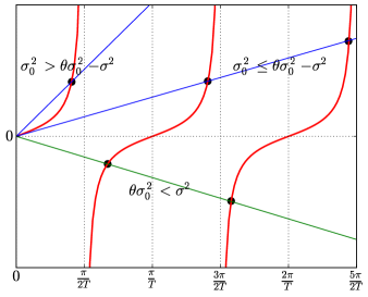
    1. (a)

      If σ2=θσ02superscript𝜎2𝜃superscriptsubscript𝜎02\sigma^{2}=\theta\sigma_{0}^{2}, Equation (7) amounts to cos(wT)=0,𝑤𝑇0\cos(wT)=0, and thus the increasingly sorted positive solutions are wn=nπTπ2Tsubscript𝑤𝑛𝑛𝜋𝑇𝜋2𝑇w_{n}=\frac{n\pi}{T}-\frac{\pi}{2T} for n1𝑛1n\geq 1.

    2. (b)

      If θσ02<σ2𝜃superscriptsubscript𝜎02superscript𝜎2\theta\sigma_{0}^{2}<\sigma^{2}, Equation (7) amounts to (σ2σ02θ)>0tan(wT)=σ02w,subscriptsuperscript𝜎2superscriptsubscript𝜎02𝜃absent0𝑤𝑇superscriptsubscript𝜎02𝑤\underbrace{\left(\sigma^{2}-\sigma_{0}^{2}\theta\right)}_{>0}\tan(wT)=-\sigma_{0}^{2}w,

      and thus the increasingly sorted positive solutions satisfy wn]nπTπ2T,nπT[subscript𝑤𝑛𝑛𝜋𝑇𝜋2𝑇𝑛𝜋𝑇w_{n}\in\left]\frac{n\pi}{T}-\frac{\pi}{2T},\frac{n\pi}{T}\right[ for n1𝑛1n\geq 1.

    3. (c)

      If θσ02>σ2𝜃superscriptsubscript𝜎02superscript𝜎2\theta\sigma_{0}^{2}>\sigma^{2}, Equation (7) amounts to (σ02θσ2)>0tan(wT)=σ02w.subscriptsuperscriptsubscript𝜎02𝜃superscript𝜎2absent0𝑤𝑇superscriptsubscript𝜎02𝑤\underbrace{\left(\sigma_{0}^{2}\theta-\sigma^{2}\right)}_{>0}\tan(wT)=\sigma_{0}^{2}w.

      There is a unique solution in each interval of the form ]kπT,kπT+π2T[𝑘𝜋𝑇𝑘𝜋𝑇𝜋2𝑇\left]\frac{k\pi}{T},\frac{k\pi}{T}+\frac{\pi}{2T}\right[ for k1𝑘1k\geq 1. There is another solution on ]0,π2T[0𝜋2𝑇\left]0,\frac{\pi}{2T}\right[ if and only if σ02>σ02θσ2superscriptsubscript𝜎02superscriptsubscript𝜎02𝜃superscript𝜎2\sigma_{0}^{2}>\sigma_{0}^{2}\theta-\sigma^{2}.

In cases (b) and (c), the numerical value can then be computed using a root-finding method on the corresponding intervals. This is illustrated in Figure 1. Using a certain rational approximation of tan\tan proposed in [5], a closed-form approximation of the solution is obtained as the root of a third-order polynomial and can be used as a starting point for the root-finding method.
Refer to caption
Figure 1: Solutions to Equation (7) in cases (b) and (c).

3 Functional quantization

The quantization of a random variable X𝑋X valued in a reflexive separable Banach space (E,||)(E,|\cdot|) consists in its approximation by Y𝑌Y that takes finitely many values in E𝐸E. We measure the resulting discretization error with the L2superscript𝐿2L^{2} norm of the difference |XY|𝑋𝑌|X-Y|. If we settle on a fixed maximum cardinal N𝑁N for Y(Ω)𝑌ΩY(\Omega), the minimization of the error reduces to the optimization problem.

N(X,||)=min{|XProjΓ(X)|2,ΓEsuch that|Γ|N},\mathcal{E}_{N}(X,|\cdot|)=\min\left\{\big{\|}\left|X-\operatorname{Proj}_{\Gamma}(X)\right|\big{\|}_{2},\ \Gamma\subset E\ \textnormal{such that}\ |\Gamma|\leq N\right\}, (8)

A solution of (8) is an L2superscript𝐿2L^{2}-optimal quantizer of X𝑋X.

Now let X𝑋X be a bi-measurable stochastic process on [0,T]0𝑇[0,T] verifying 0T𝔼[|Xt|2]𝑑t<superscriptsubscript0𝑇𝔼delimited-[]superscriptsubscript𝑋𝑡2differential-d𝑡\int_{0}^{T}\mathbb{E}\left[|X_{t}|^{2}\right]dt<\infty, which we see as a random variable valued in the Hilbert space H=L2([0,T])𝐻superscript𝐿20𝑇H=L^{2}([0,T]). We assume that its covariance function ΓXsuperscriptΓ𝑋\Gamma^{X} is continuous. In the seminal paper [10], it is shown that, in the centered Gaussian case, linear subspaces U𝑈U of H𝐻H spanned by N𝑁N-stationary quantizers correspond to principal components of X𝑋X, in other words, are spanned by eigenvectors of the covariance operator of X𝑋X, that is, its Karhunen-Loève eigenfunctions (enX)n1subscriptsuperscriptsubscript𝑒𝑛𝑋𝑛1\left(e_{n}^{X}\right)_{n\geq 1}.

To perform optimal quantization, the Karhunen-Loève expansion is first truncated at a fixed order m𝑚m and then the msuperscript𝑚\mathbb{R}^{m}-valued Gaussian vector constituted of the m𝑚m first coordinates of the process on its Karhunen-Loève decomposition is quantized. We have to determine the optimal rank of truncation dX(N)superscript𝑑𝑋𝑁d^{X}(N) (the quantization dimension) and the optimal dX(N)superscript𝑑𝑋𝑁d^{X}(N)-dimensional quantizer of the first coordinates, j=1dX(N)𝒩(0,λjX)superscriptsubscripttensor-product𝑗1superscript𝑑𝑋𝑁𝒩0subscriptsuperscript𝜆𝑋𝑗\bigotimes\limits_{j=1}^{d^{X}(N)}\mathcal{N}\left(0,\lambda^{X}_{j}\right). The minimal quadratic distortion N(X)subscript𝑁𝑋\mathcal{E}_{N}(X) is given by

N(X)2=jm+1λjX+N(j=1m𝒩(0,λjX))2.subscript𝑁superscript𝑋2subscript𝑗𝑚1superscriptsubscript𝜆𝑗𝑋subscript𝑁superscriptsuperscriptsubscripttensor-product𝑗1𝑚𝒩0superscriptsubscript𝜆𝑗𝑋2\mathcal{E}_{N}(X)^{2}=\sum\limits_{j\geq m+1}\lambda_{j}^{X}+\mathcal{E}_{N}\bigg{(}\bigotimes\limits_{j=1}^{m}\mathcal{N}\left(0,\lambda_{j}^{X}\right)\bigg{)}^{2}.

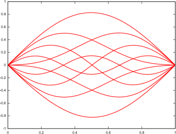
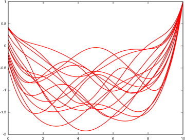
If the eigensystem (enX,λnX)1ndX(N)subscriptsuperscriptsubscript𝑒𝑛𝑋superscriptsubscript𝜆𝑛𝑋1𝑛superscript𝑑𝑋𝑁\left(e_{n}^{X},\lambda_{n}^{X}\right)_{1\leq n\leq d^{X}(N)} is known, we just need to perform the finite-dimensional quantization of j=1m𝒩(0,λjX)superscriptsubscripttensor-product𝑗1𝑚𝒩0superscriptsubscript𝜆𝑗𝑋\bigotimes\limits_{j=1}^{m}\mathcal{N}\left(0,\lambda_{j}^{X}\right). Various algorithms have been devised to deal with this problem, among others, Lloyd’s algorithm [9] and the Competitive Learning Vector Quantization (CLVQ) [12]. In Figures 2 and 3, we show optimal quantizers of the Orntein-Uhlenbeck bridge for different initial variances, mean-reversion parameters, volatilities and maturities.
Refer to caption
Figure 2: Optimal quantization of the Ornstein-Uhlenbeck bridge with parameters T=1𝑇1T=1, θ=1𝜃1\theta=1, σ2=1superscript𝜎21\sigma^{2}=1, σ02=0subscriptsuperscript𝜎200\sigma^{2}_{0}=0, x0=μ=XT=0subscript𝑥0𝜇subscript𝑋𝑇0x_{0}=\mu=X_{T}=0 and N=10𝑁10N=10.
Refer to caption
Figure 3: Optimal quantization of the Ornstein-Uhlenbeck bridge with parameters T=10𝑇10T=10, θ=1𝜃1\theta=1, σ2=1superscript𝜎21\sigma^{2}=1, σ02=1/2superscriptsubscript𝜎0212\sigma_{0}^{2}=1/2, x0=0subscript𝑥00x_{0}=0, μ=1𝜇1\mu=-1, XT=1subscript𝑋𝑇1X_{T}=1 and N=16𝑁16N=16.

Moreover, using the rate of decay of the Karhunen-Loève eigenvalues of the Ornstein-Uhlenbeck bridge, and [11, Theorem 2.22.22.2], we see that the optimal quadratic quantization error of level N𝑁N of the Ornstein-Uhlenbeck bridge N(X)subscript𝑁𝑋\mathcal{E}_{N}(X) satisfies N(X)Klog(N)1/2\mathcal{E}_{N}(X)\sim K\log(N)^{-1/2} as N𝑁N\to\infty, for some K>0𝐾0K>0.

References

  • [1] L. Alili. Canonical decompositions of certain generalized Brownian bridges. Electronic communications in probability, 7:27–35, 2002.
  • [2] M. Barczy and E. Iglói. Karhunen-Loève expansions of α𝛼\alpha-Wiener bridges. Central European Journal of Mathematics, 9(1):65–84, 2011.
  • [3] M. Barczy and P. Kern. Representations of multidimensional linear process bridges. Random Opeators and Stochastic Equations, 21:159–189, 2013.
  • [4] S. Corlay. Partial functional quantization and generalized bridges. To appear in Bernoulli Journal, 2011.
  • [5] S. Corlay and G. Pagès. Functional quantization-based stratified sampling methods. Preprint, 2010.
  • [6] A. Daniluk and R. Muchorski. The approximation of bonds and swaptions prices in a Black-Karasiński Model based on the Karhunen-Loève expansion. In 6th General AMaMeF and Banach Center Conference, 2013.
  • [7] P. Deheuvels and G. V. Martynov. A Karhunen-Loève decomposition of a Gaussian process generated by independent pairs of exponential random variables. Journal of Functional Analysis, 255(9):2363–2394, 2008.
  • [8] X. Fernique. Intégrabilité des vecteurs gaussiens. Comptes rendus de l’Académie des sciences, 1970.
  • [9] S. P. Lloyd. Least squares quantization in PCM. Information Theory, IEEE Transactions on, 28(2):129–137, 1982.
  • [10] H. Luschgy and G. Pagès. Functional quantization of Gaussian processes. Journal of Functional Analysis, 196(2):486–531, 2002.
  • [11] H. Luschgy and G. Pagès. Sharp asymptotics of the functional quantization problem for Gaussian processes. Annals of Probability, 32(2):1574–1599, 2004.
  • [12] G. Pagès and J. Printems. Optimal quadratic quantization for numerics: the Gaussian case. Monte Carlo Methods and Applications, 9:135–166, 2003.