Single-field inflation à la generalized Chaplygin gas

Abstract

In the simplest scenario for inflation, i. e. in the single-field inflation, it is presented an inflaton field with properties equivalent to a generalized Chaplygin gas. Their study is performed using the Hamilton-Jacobi approach to cosmology. The main results are contrasted with the measurements recently released by the Planck data, combined with the WMAP large-angle polarization. If the measurements released by Planck for the scalar spectral index together with its running are taken into account it is found a value for the $\alpha$-parameter associated to the generalized Chaplygin gas given by $\alpha=0.2578\pm 0.0009$.

I Introduction

The inflationary paradigm has been proposed as a good approach for solving most of the cosmological ”puzzles” (linde90a, ). Apart of solving these cosmological problems, inflation produces the seeds that, in the course of the subsequent eras of radiation and matter dominance, developed into the cosmic structures (galaxies and clusters thereof) that we observe today. In fact, the present popularity of the inflationary scenario is entirely due to its ability to generate a spectrum of density perturbations which lead to structure formation in the universe. In essence, the conclusion that all the observations of microwave background anisotropy performed so far support inflation, rests on the consistency of the anisotropy with an almost Harrison-Zel’dovich power spectrum predicted by most of the inflationary universe scenarios (WMAP03, ) and corroborated by the measurements recently released by the Planck combined with the WMAP large-angle polarizationPlanck2013 .

The essential feature of any inflationary universe model proposed so far is the rapid (accelerated) but finite period of expansion that the universe underwent at very early times in its evolution. The implementation of the inflationary universe model rests on the introduction of a scalar inflaton field, $\phi$. The evolution of this field becomes governed by its scalar potential, $V(\phi)$, via the Klein-Gordon equation. Thus, this equation of motion, together with the Friedmann equation, obtained from Einstein general relativity theory, form the most simple set of field equations, which could be applied to obtain inflationary solutions. But, in order to do this it is necessary to give an explicit expression for the scalar inflaton potential $V(\phi)$. However, in simple cases result very complicated to find solutions, even in the situation in which it is applied the so-called slow-roll approximation, where the kinetics terms is much smaller than the potential energy, i.e. $\dot{\phi}^{2}\ll V(\phi)$, together with the approximation $\mid\ddot{\phi}\mid\ll H\mid\dot{\phi}\mid$. This approach is usually refereed as the single-field inflation, whose definition encompasses the type of models where the inflationary phase becomes described by a single inflaton scalar field.

One way of finding inflationary solutions out of the slow-roll approximation is giving the functional form of the Hubble parameter in term of the inflaton field, i.e. $H(\phi)$, the so called generating fuctionL91 . This approach presents some advantages when compared with the slow-roll approximation: first of all, the form of the potential is deduced, and secondly, since an exact solution is obtained, then, application to the final period of inflation is possible. We should note that in this period the kinetic term associated to the inflaton field in the Friedmann equation becomes important. Certainly, this approach becomes necessary when studying the final stage of inflation, i.e. during the reheating phase. This method, that we will consider here, is usually referred as the Hamilton-Jacobi scheme to cosmologyGS88 ; LetAl97 ; dC12 .

In this paper we would like to study the consequences of considering an inflationary universe model in which the inflaton field presents characteristic of a generalized Chaplygin gasB01 ; B02 ; G03 ; B04 , with Equation of state

$$p_{\phi}=-B\rho_{\phi}^{-\alpha},$$ (1)

where $B$ is a positive constant and $\alpha$ a parameter that we call the generalizes Chaplygin gas parameter, which will be considered to lie in the range $0<\alpha<1$, and $p_{\phi}$ and $\rho_{\phi}$ are defined, as usual, by expressions $p_{\phi}\equiv\frac{1}{2}\,\dot{\phi}^{2}-V(\phi)$ and $\rho_{\phi}\equiv\frac{1}{2}\,\dot{\phi}^{2}+V(\phi)$, respectively. The usual Chaplygin gas is obtained when the parameter $\alpha$ becomes equal to one. Because the range that we have set for this parameter does not provide equality we will not include the possibility of considering the usual Chaplygin gas in our analysis. Moreover, it is possible to extend our analysis to include values of the parameter $\alpha$ which lie outside the range specified above, even by taking negative values, but our results do not change much. For simplicity, we shall restrict ourselves to considerer this parameter to lie in the range that we have specified above.

The sort of matter related to the usual Chaplygin gas, and its generalizations, have been extensively studied, and considered as one of the main matter components of the universe at present timeKMP . It has been established that this kind of component could be considered as the unification of dark matter and dark energyB01 . On the other hand, the relation between a perfect fluid, which can be related to a Chaplygin gas together with the corresponding scalar field models were considered in RefsPMT04 ; GKMPS05 ; U13 . The different parameters that enter into the model have been confronted with the recent observational data coming out of gravitational lensing, the baryon acoustic oscillation, the Cosmic Microwave Background Radiation from the Wilkinson Microwave Anisotropy Probe (WMAP7) resultL11 , Gamma-ray burstsF11 , power spectrum observational dataFa11 , the Constitution data set of type supernovae Ia cosmic probes, together with sample of cosmology-independent long gamma-ray bursts calibrated using their Type I Fundamental Plane, as well as the Union 2.1 set and observational Hubble parameter dataL12 , the combination of Chandra observations of the x-ray luminosity of galaxy clusters, together with independent measurements of the baryonic matter density, the latest measurements of the Hubble parameter as given by the HST Key Project, and data of the Supernova Cosmology ProjectC04 . Also, it was applied the the statefinder parametersS03 . Furthermore, combinations of some of these measurements have been made as wellW13 . On the other hand, the generalized Chaplygin gas has been studied by considering non-adiabatic pressure perturbations, where it was found that there are no instabilities which have been found in previous adiabatic Chaplygin-gas modelsB13 . Also, a successful description was obtained for generalized Chaplygin gas in thawing modelsdC13 .

One of the interesting features of the generalize Chaplygin gas is the connection that it has with string theory. Effectively, it can be obtained from the Nambu-Goto action for a D-brane moving in a (D+1,1)-dimensional spacetime in the light cone parametrizationvarios01 . This open a window for applying this sort of theory at early time in the evolution of the universe. The idea of taking an early phase of the universe in which the main component corresponds to a Chaplygin gas has been considered in Ref. varios001 . The tachyon-Chaplygin inflationary universe model was studied in Ref. dC08 under the slow-roll approximation.

The out line of this paper is as follows. We first describe exact solutions to inflationary universe models within the framework of the so-called Hamilton-Jacobi approach to cosmology. This will be carried out in section II. Then, in section III we apply this approach to the generalized Chaplygin gas inflationary universe model. In section IV we study the corresponding scalar and tensor perturbations. Finally, we conclude our work in section V.

II The Hamilton-Jacobi approach to inflation

The simplest model that describes inflationary universes in general relativity presents two main ingredients: the flat FRW metric and the single inflaton scalar field, $\phi$.

In the scheme of Hamilton-Jacobi approach the fundamental Equations of the model are described by the Klein-Gordon Equation, which satisfies the inflaton scalar field and it given by

$$\ddot{\phi}+3H\dot{\phi}+V^{\prime}(\phi)=0,$$ (2)

where $V^{\prime}$ represents a derivative with respect to $\phi$, and the Friedmann Equation given by

$$H^{2}=\frac{8\pi}{3\,m_{Pl}^{2}}\left[\frac{1}{2}\dot{\phi}^{2}+V(\phi)\right].$$ (3)

Here, $m_{Pl}^{2}=1/G$ is the Planck mass.

It is not hard to see from Eqs. (2) and (3) that the following relationship is satisfied

$$\dot{\phi}=-\,\left(\frac{m_{Pl}^{2}}{4\pi}\right)\,H^{\prime},$$ (4)

where $H^{\prime}$ represents a derivative with respect to $\phi$. Since it is assumed that the generating function $H(\phi)$ it is known, we can add that this latter relation allows us to obtain an explicit expression for the inflaton field in terms of the cosmological time $t$ in cases where it is possible to reverse the expression of the scalar field, $\phi$.

Also, it is not hard to see that it is found that

$$a\,H=-\left(\frac{m_{Pl}^{2}}{4\,\pi}\right)\,a^{\prime}\,H^{\prime},$$ (5)

from which we get that

$$a(\phi)=\exp\left\{-\frac{4\,\pi}{m_{Pl}^{2}}\,\int\frac{H}{H^{\prime}}\,d\phi\right\},$$ (6)

i.e. the scale factor $a$ as a function of the inflaton field $\phi$, and thus, assuming that we have the scalar field as a function of time, then we can obtain the scale factor as a function of the cosmological time.

The scalar potential $V(\phi)$ becomes given by

$$V(\phi)=\left(\frac{3\,m_{Pl}^{2}}{8\,\pi}\right)\left[H^{2}-\frac{3\,m_{Pl}^{2}}{12\,\pi}\left(H^{\prime}\right)^{2}\right].$$ (7)

We should note that in the slow-roll approximation this potential becomes $\displaystyle V(\phi)\simeq\left(\frac{3\,m_{Pl}^{2}}{8\,\pi}\right)\,H^{2}$

On the other hand, we see that the acceleration Equation for the scale factor results to be

$$\frac{\ddot{a}}{a}=H^{2}\left[1-\epsilon_{{}_{H}}\right],$$ (8)

where the function $\epsilon_{{}_{H}}$ corresponds to

$$\epsilon_{{}_{H}}\equiv-\frac{d\ln{H}}{d\ln{a}}=\left(\frac{m_{{}_{Pl}}^{2}}{4\,\pi}\right)\,\left(\frac{H^{\prime}}{H}\right)^{2}.$$ (9)

From this latter expression we can see that this definition, called the first Hubble hierarchy parameter, gives information about the acceleration of the universe. During inflation this parameter satisfies the bound $\epsilon_{{}_{H}}<1$, and inflation ends when $\epsilon_{{}_{H}}$ takes the value equal to one. In the next section we will use this parameter for describing scalar and tensor perturbations.

One interesting quantity in characterizing inflationary universe models is the amount of inflation. Usually, this quantity is defined by

$$N(t)\equiv\ln{\frac{a\left(t_{end}\right)}{a(t)}},$$ (10)

where $a\left(t_{end}\right)$ corresponds to the scale factor evaluated at the end of inflation. By considering expressions (4) and (9) we write

$$N(\phi)\equiv\int_{t}^{t_{end}}{H\,dt}=\left(\frac{4\,\pi}{m_{{}_{Pl}}^{2}}\right)\int^{\phi}_{\phi_{end}}\frac{H}{H^{\prime}}\,d\phi=\int^{\phi}_{\phi_{end}}\frac{1}{\epsilon_{{}_{H}}}\,\frac{H^{\prime}}{H}\,d\phi.$$ (11)

Here, $\phi_{end}$ represent the value of the scalar field at the end of inflation. Its value is determined by imposing that $\epsilon_{{}_{H}}\left(\phi_{end}\right)=1$. We interpret the parameter $N$ as the number of e-folding before inflation ends.

It seems to be more appropriated to describe the amount of inflation in terms of the comoving Hubble length, $1/(aH)$ than in terms of the scale factor only. In this case the amount of inflation becomesLPB94

$$\overline{\text{N}}=\ln{\frac{a\left(t_{end}\right)\,H\left(t_{end}\right)}{a(t)\,H(t)}},$$ (12)

which results into

$$\overline{\text{N}}(\phi)=\int^{\phi}_{\phi_{end}}\left(\frac{1}{\epsilon_{{}_{H}}}-1\right)\,\frac{H^{\prime}}{H}\,d\phi.$$ (13)

Note that, in general, $\overline{\text{N}}(\phi)$ is smaller that $N(\phi)$ and only in the slow-roll limit they coincide. In the following, and for simplicity, we will restrict ourselves to consider the amount of inflation given by $N(\phi)$.

In the description of inflation it is convenient to show that their solutions are independent from their initial conditions. This ensure the true predictive power that presents any inflationary universe model, otherwise the corresponding physical quantities associated with the inflationary phase, such that the scalar or tensor spectra, would depend on these initial conditions. Thus, with the purpose of being predictive, any inflationary model needs that their solutions present an attractor behavior, in the sense that solutions with different initial conditions should tend to a unique solutionSB90 .

Let us start by considering a linear perturbation, $\delta H(\phi)$, around a given inflationary solution, expressed by $H_{0}(\phi)$. In the following we will refer to this quantity as the background solution, and any quantity with the subscript zero is assumed to be evaluated taking into account the background solution. Therefore, at first order on $\delta H(\phi)$, we get from the field Equations (2) and (3) that

$$\delta H\simeq\left.\frac{1}{3}\left(\frac{m_{{}_{Pl}}^{2}}{4\pi}\right)\frac{H^{\prime}}{H}\right|_{0}\delta H^{\prime},$$ (14)

This latter expression can be solved for getting

$$\delta H(\phi)=\delta H(\phi_{{}_{i}})\exp\int_{\phi_{{}_{i}}}^{\phi}\left.\left(\frac{3}{\epsilon_{{}_{H}}}\right)\frac{H^{\prime}}{H}\right|_{0}d\phi,$$ (15)

where $\phi_{{}_{i}}$ corresponds to some arbitrary initial value of $\phi$. Since $d\phi$ and $H^{\prime}$ have opposite signs (assuming that $\dot{\phi}$ does not change sign due to the perturbation $\delta H$) the linear perturbations tend to vanish quicklyLPB94 .

In the following we want to apply this scheme to the case in which the inflaton field corresponds to a generalized Chaplygin gas fluid whose equation of state is governed by expression (1).

III Inflation à la Chaplygin

In this section we describe the inflationary model by using a fluid which presents the properties of a generalized Chaplygin gas, where the equation of state of this fluid corresponds to that specified by equation (1). In order to do this we start by taking that the generating function, $H(\phi)$ is given by

$$H(\phi)=H_{0}\cosh^{\frac{1}{1+\alpha}}\left[\sqrt{\frac{6\pi}{m_{Pl}^{2}}}(1+\alpha)(\phi-\phi_{0})\right],$$ (16)

where $H_{0}$, the value of $H$ when $\phi=\phi_{0}$, is a constant given by $\displaystyle H_{0}=\sqrt{\frac{8\pi}{3\,m_{Pl}^{2}}}\,B^{\frac{1}{2(1+\alpha)}}$, with $B$ and $\alpha$ introduced previously in Eq. (1). For simplicity from now on we will use the following dimensionless variable as the inflaton scalar field: $\Phi(\phi)\equiv\sqrt{\frac{6\pi}{m_{Pl}^{2}}}(\phi-\phi_{0})$.

In order to see that the expression above corresponds to a fluid which has an equation of state related to a Chaplygin gas, we take into account that the pressure and the energy density are given by

$$p_{\phi}=\frac{3m_{Pl}^{2}}{8\pi}\,H^{2}\left[\frac{m_{Pl}^{2}}{6\pi}\,\left(\frac{H^{\prime}}{H}\right)^{2}-1\right]$$ (17)

and

$$\rho_{\phi}=\frac{3m_{Pl}^{2}}{8\pi}\,H^{2},$$ (18)

respectively. Now, by using Eq. (16) into these two latter Equations we obtain that

$$p_{\phi}=-\frac{3m_{Pl}^{2}}{8\pi}\,H_{0}^{2}\,\cosh^{-\frac{2\alpha}{1+\alpha}}\left[(1+\alpha)\Phi\right]$$ (19)

and

$$\rho_{\phi}=H_{0}^{2}\cosh^{\frac{2}{1+\alpha}}\left[(1+\alpha)\Phi\right],$$ (20)

respectively. From Eq. (20) we get $\displaystyle\cosh\left[(1+\alpha)\Phi\right]$ as a function of $\rho_{\phi}$ and then substituting into Eq. (19) we obtain the Equation of state related to the generalized Chaplygin gas, as expressed by Eq. (1). In this way, the generating function expressed by Eq. (16) corresponds effectively to a generalized Chaplygin gas generating function.

From Eq. (4) together with Eq. (16) we get that

$$\csc^{\frac{1}{1+\alpha}}\left[(1+\alpha)\Phi\right]{}_{2}F_{1}\left[\frac{1}{2(1+\alpha)},\frac{1}{2(1+\alpha)};\frac{3+2\alpha}{2(1+\alpha)};-\csc^{2}\left[(1+\alpha)\Phi\right]\right]=-\sqrt{\frac{3m_{Pl}^{2}}{8\pi}}\,H_{0}t,$$ (21)

where ${}_{2}F_{1}\left[a,b;c;z\right]$ represents the hypergeometric function. This latter expression gives information on how the inflaton field evolves with the cosmological time. In the same way we get that the scale factor, $a(t)$, results to be given by

$$a(\phi)=a_{i}\left(\frac{\sinh\left[(1+\alpha)\Phi\right]}{\sinh\left[(1+\alpha)\Phi_{i}\right]}\right)^{\frac{2}{3}},$$ (22)

where $a_{i}$ is the value of the scale factor when the inflaton field has the value $\phi_{i}$, and $\Phi_{i}=\Phi(\phi_{i})$.

In order to see that we have an inflationary period, we introduce the deceleration parameter $q$, defined as $\displaystyle q=-\frac{\ddot{a}\,a}{\dot{a}^{2}}$, which in terms of the Hubble parameter it becomes $\displaystyle q=\left(\frac{m_{Pl}^{2}}{4\pi}\right)\,\left(\frac{H^{\prime}}{H}\right)^{2}-1$, which gives

$$q=-1+\frac{3}{2}\,\tanh^{2}\left[(1+\alpha)\Phi\right].$$ (23)

We note that this quantity becomes negative for the values $\displaystyle\phi\leq\phi_{0}\,\pm\,\frac{1}{1+\alpha}\sqrt{\frac{1}{6\,\pi}}\,{\text{arctanh}}\left(\sqrt{\frac{2}{3}}\right)\,m_{Pl}$. The equal sign corresponds to when the $q$ parameter vanishes, i.e. when inflation ends. Figure 1 shows how the parameter $q$ changes as a function of the dimensionless field $\Phi$. There, we have taken two different values of the parameter $\alpha$. The dot-dashed line corresponds to the value $\alpha=0.2$ and the continuous line to $\alpha=0.8$. These curves show that the universe is accelerating, since the parameter $q$ turns out to be negative, at least for the values that we have considered here.

Figure 1: The deceleration parameter $q$ as a function of the dimensionless scalar field $\Phi\equiv\sqrt{\frac{6\pi}{m^{2}_{Pl}}}\,(\phi-\phi_{0})$. Here we have taken the values for the generalized Chaplygin gas parameter $\alpha=0.2$ (dot-dashed line) and $\alpha=0.8$ (solid line).

From expressions (7) together with Eq. (16) we obtain for the scalar potential

$$V(\phi)=\,V_{0}\cosh^{-\frac{2\,\alpha}{1+\alpha}}\,\left[(1+\alpha)\Phi\right]\left(1+\cosh^{2}\left[(1+\alpha)\Phi\right]\right),$$ (24)

where $V_{0}=\frac{1}{2}B^{\frac{1}{1+\alpha}}$. In the slow-roll approximation, i.e. when $\dot{\phi}^{2}\ll V(\phi)$ together with $\mid\ddot{\phi}\mid\ll\mid dV(\phi)/d\phi\mid$, the scalar potential reduces to

$$V_{{}_{s-r}}(\phi)\simeq V_{0}\cosh^{\frac{2}{1+\alpha}}\,\left[(1+\alpha)\Phi\right].$$ (25)

Figure 2: Plots of the scalar potentials, $V(\Phi)$, as a function of the dimensionless scalar field, $\Phi\equiv\sqrt{\frac{6\pi}{m^{2}_{Pl}}}\,(\phi-\phi_{0})$. The solid line represents the scalar potential, expressed by Eq. (24) for the value $\alpha=0.2$. The dot-dashed line represents the same potential, but for the value $\alpha=0.8$. The scalar potential $V(\Phi)$ is expressed as a multiple of the constant $\displaystyle V_{0}\equiv\frac{1}{2}B^{\frac{1}{1+\alpha}}$.

Figure 2 depicts the shape of the potential for the exact case, expressed by Eq. (24) as a function of the dimensionless scalar field $\Phi$. Here, we have plotted the potential for two values of the parameter $\alpha$. The dot-dashed and the solid lines correspond to $\alpha=0.8$ and $\alpha=0.2$, respectively.

One interesting quantity in characterizing inflationary universe models is the amount of inflation. This quantity was introduced above (see Eq. (10)) and together with expression (22) we obtain that

$$N(\phi)=\frac{2}{3}\,\ln\left\{\frac{\sinh\left[(1+\alpha)\Phi_{e}\right]}{\sinh\left[(1+\alpha)\Phi\right]}\right\},$$ (26)

where $\Phi_{e}=\Phi(\phi_{e})$, with $\phi_{e}$ representing the value of the inflaton field at the end of inflation. This value is obtained by demanding that the first Hubble hierarchy parameter $\epsilon_{{}_{H}}$ becomes equal to one at the end of inflation. This parameter becomes determined by considering its definition, Eq. (9), together with expression (16)

$$\epsilon_{{}_{H}}(\phi)=\frac{3}{2}\,\tanh^{2}\,\left[(1+\alpha)\Phi\right].$$ (27)

Now, requiring that $\epsilon_{{}_{H}}(\phi_{e})=1$ we get that for the dimensionless scalar field $\displaystyle\Phi_{e}=\frac{1}{1+\alpha}\text{arctanh}\left(\sqrt{\frac{2}{3}}\right)$, or equivalently, for the inflaton field, $\phi_{e}=\phi_{0}\,\pm\,\frac{1}{1+\alpha}\sqrt{\frac{1}{6\,\pi}}\,{\text{arctanh}}\left(\sqrt{\frac{2}{3}}\right)\,m_{Pl}$. Note that, as specified above, this value coincides with that obtained when the parameter $q$ gets vanished, i.e. when inflation ends.

To study the attractor behavior of the model we consider a linear perturbation, $\delta H(\phi)$, around a given solution, just as was specified above. Thus, from Equations (15), (16) and (27) we get that

$$\delta H(\phi)=\left(\frac{\sinh\left[(1+\alpha)\Phi_{i}\right]}{\sinh\left[(1+\alpha)\Phi\right]}\right)^{\frac{2}{1+\alpha}}\delta H(\phi_{{}_{i}}).$$ (28)

Here, it is assumed that $\Phi\geq\Phi_{i}$ is satisfied, and thus, the ratio $\displaystyle\frac{\sinh\left[(1+\alpha)\Phi_{i}\right]}{\sinh\left[(1+\alpha)\Phi\right]}$ decreases rapidly, as the scalar field $\Phi$ increases. In this way, the linear perturbation tends to vanish rapidly. This can be seen more clearly, since the factor accompanying to $\delta H(\phi_{{}_{i}})$ is nothing but $(a/a_{i})^{-\frac{3}{1+\alpha}}$ (see expression (22)), which during inflation the quantity in this bracket increases at least 70 e-fold, leaving $\delta H(\phi)$ very small.

IV Scalar and tensor perturbations

Quantum fluctuations are amplified during inflation. They are stretched to astrophysical scales by the rapid expansion that universe presents at early time. In general terms any model of inflation generate two types of perturbations, density perturbations (which come from quantum fluctuations in the scalar field, together with the corresponding scalar metric perturbationMCh81 ; L80 ), and relic gravitational waves which are tensor metric fluctuationsG75 . The former experience gravitational instability and lead to structure formationMFB92 , while the latter predicts a stochastic background of relic gravitational waves which could influence the cosmic microwave background anisotropy via the presence of polarization in itGW .

In order to describe these perturbations we need to introduce a series of parameters which are known as the Hubble hierarchy parameters. We have already defined one of them, the so-called first Hubble hierarchy parameter, which is expressed by expression (27). The second Hubble hierarchy parameter, $\eta_{{}_{H}}$, is defined by

$$\eta_{{}_{H}}\equiv-\frac{d\,\ln H^{\prime}}{d\,\ln a}=\frac{m_{Pl}^{2}}{4\,\pi}\,\left(\frac{H^{\prime\prime}}{H}\right),$$ (29)

from which we get that for the generalized Chaplygin gas it becomes

$$\eta_{{}_{H}}=\frac{3}{4}\,\left(1+2\alpha+\cosh\left[2\,(1+\alpha)\Phi\right]\right)\,{\text{ sech}}^{2}\left[(1+\alpha)\Phi\right].$$ (30)

The third Hubble hierarchy parameter, $\xi_{{}_{H}}^{2}$ is defined by

$$\xi_{{}_{H}}^{2}\equiv\left(\frac{m_{{}_{Pl}}^{2}}{4\,\pi}\right)^{2}\,\left(\frac{H^{\prime\prime\prime}\,H^{\prime}}{H^{2}}\right),$$ (31)

which results to be

$$\xi_{{}_{H}}^{2}=\frac{9}{8}\,\left(1-2\alpha-4\,\alpha^{2}\right. \left.+\cosh\left[2\,(1+\alpha)\Phi\right]\right)$$

$$\times{\text{ sech}}^{2}\left[(1+\alpha)\Phi\right]\,\tanh^{2}\left[(1+\alpha)\Phi\right]$$ (32)

The evolution equation for the Fourier modes of the scalar perturbations at some scale $k$, corresponding to a comovil wave number, is governed by the following Equationvarios03

$$\frac{d^{2}u_{k}}{d\eta^{2}}+\left(k^{2}-\frac{1}{z}\frac{d^{2}z}{d\eta^{2}}\right)u_{k}=0,$$ (33)

where $\eta$ represents the conformal time defined by $\eta=\int{\frac{1}{a}\,dt}$ and $u_{k}$ corresponds to the Fourier transformed of the Mukanov variable, which is defined by $u=z\cal{R}$, with $z=a\frac{\dot{\phi}}{H}$ and $\cal{R}$ represents the gauge-invariant comovil curvature perturbation. This latter amount remains constant outside the horizon, i.e. metric perturbations with wavelengths larger than the Hubble radius1983 . The term $\frac{1}{z}\frac{d^{2}z}{d\eta^{2}}$ is usually refereed as the ”mass term”.

During inflation we have that $k^{2}\gg\frac{1}{z}\frac{d^{2}z}{d\eta^{2}}$, i.e. it is assumed that the physical mode has a wavelength much smaller than the curvature scale. Eq. (33) presents a solution of the type

$$u_{k}(\eta)\sim e^{-ik\eta}\left(1+\frac{{\cal{A}}_{k}}{\eta}+....\right).$$ (34)

Contrary, when $k^{2}\ll\frac{1}{z}\frac{d^{2}z}{d\eta^{2}}$, the physical modes present wavelengths much bigger than the curvature scale. The term $\frac{1}{z}\frac{d^{2}z}{d\eta^{2}}$ it is found to beSL93 .

$$\frac{1}{z}\frac{d^{2}z}{d\eta^{2}}=2a^{2}H^{2}\left\{1+\epsilon_{{}_{H}}-\frac{3}{2}\eta_{{}_{H}}-\frac{1}{2}\epsilon_{{}_{H}}\eta_{{}_{H}}+\frac{1}{2}\eta_{{}_{H}}^{2}+\frac{1}{2H}\dot{\epsilon}_{{}_{H}}-\frac{1}{2H}\dot{\eta}_{{}_{H}}\right\},$$ (35)

It is well known that Eq. (33) solves exactly when $\frac{1}{z}\frac{d^{2}z}{d\eta^{2}}$ is proportional to $\eta^{-2}$, in which case Eq. (33) reduces to a Bessel equation, where the solution becomes $u_{k}\sim\sqrt{-k\tau}H_{\nu}(-k\tau)$, with $H_{\nu}$ the Hankel function of first kind, and the parameter $\nu$ depends on the slow-roll parameter $\epsilon$ via $\nu=3/2+\epsilon/(1-\epsilon)$. This happens when the scale factor expands as a power law, i.e. $a(t)\sim t^{p}\,\,(p>1)$. Here, it is obtained that $\epsilon_{{}_{H}}=\eta_{{}_{H}}=\text{Constant}$LS92 . Others solutions, far from the slow-roll approximation, are described in Ref. K97 . In the generalized Chaplygin gas case this issue becomes more subtle and needs to be worked numerically.

The power spectrum becomes defined in terms of the two point correlation function as

$${\cal{P}}_{\cal{R}}(k)=\frac{k^{3}}{2\pi^{2}}<{\cal{R}}_{{\overrightarrow{k}^{\prime}}}{\cal{R}}_{{\overrightarrow{k}}}>\delta(\overrightarrow{k}^{\prime}+\overrightarrow{k}),$$ (36)

which in terms of the $u_{k}$ and $z$ it becomes

$${\cal{P}}_{\cal{R}}(k)=\frac{k^{3}}{2\pi^{2}}\left|\frac{u_{k}}{z}\right|^{{}^{2}}.$$ (37)

By solving equation (33) it is needed to impose boundary conditions to the solutions. Asymptotic conditions are usually consider to be the so-called Bunch-Davies vacuum stateK12

$$u_{k}\rightarrow\left\{\begin{array}[]{lll}\frac{1}{\sqrt{2k}}e^{-ik\eta}&\hskip 14.22636pt$as$&-k\eta\longrightarrow\infty,\\ {\cal{A}}_{k}z&\hskip 14.22636pt$as$&-k\eta\longrightarrow 0.\end{array}\right.$$ (38)

This ensures that perturbations that are generated well inside the horizon, i.e. in the region where $k\ll aH$, the modes approach plane waves and those that are generated well outside the horizon, i.e. in the region where $k\gg aH$, are fixed.

The primordial curvature perturbation are given byHa82 ; varios02

$${\cal{P}}_{\cal{R}}(k)=\left.\left(\frac{H}{|\dot{\phi}|}\right)^{2}\,\left(\frac{H}{2\,\pi}\right)^{2}\right|_{aH=k}.$$ (39)

This perturbation is evaluated for $aH=k$, i.e. when a given mode crosses outside the horizon during inflation. We should notice that the modes do not evolve outside the horizon, therefore, they kept a fixed value after crossing the horizon during inflation. Certainly, this value coincides with that amplitude when they cross back inside the horizon during a later epoch.

We can introduce the scalar spectral index $n_{s}$ defined by

$$n_{s}-1\equiv\frac{d\ln{\cal{P}}_{\cal{R}}}{d\ln{k}}.$$ (40)

It is not hard to see that this quantity becomes

$$n_{s}-1=2\eta_{{}_{H}}-4\,\epsilon_{{}_{H}}.$$ (41)

By using expression (16) we obtain that

$$n_{s}-1=\frac{3}{2}\left(3+2\,\alpha-\cosh\left[2\,(1+\alpha)\Phi\right]\right)\,\text{sech}^{2}\left[(1+\alpha)\Phi\right].$$ (42)

It is not hard to see that $n_{s}$ gets the value equal to one when the dimensionless scalar field becomes either too big, in which case the sech-factor becomes vanishes, or when it gets the value $\displaystyle\Phi_{n_{s}=1}=\frac{1}{2(1+\alpha)}\,\text{arccosh}(3+2\alpha)$. The former case is unfeasible, since the inflaton field is bounded from above, i.e. $\Phi\leq\Phi_{e}$. We notice that the ratio between $\Phi_{e}$ and $\Phi_{n_{s}=1}$ depends on the parameter $\alpha$, and since we have considered that this parameter is located in the range $0<\alpha<1$, we get that this ratio gets an upper bound $\left(\frac{\Phi_{e}}{\Phi_{n_{s}=1}}\right)\,<\,1.0\,(\text{for}\,\alpha=1)\,\text{or}\,\left(\frac{\Phi_{e}}{\Phi_{n_{s}=1}}\right)\,<\,1.3\,(\text{for}\,\alpha=0)$. Thus, we see that they becomes closer each other when the parameter $\alpha$ gets closer to one. From this we see that this model favors a model of inflation which does not present a Harrison-Zeld dovic spectrum, unless the parameter $\alpha$ gets the value equal to one. This result is in agreement with the conclusion reached by Planck, which rules out exact scale invariance at over $5\sigma$. As we shall see, by using the data realized by Planck for the scalar spectral index, together with its running, will give a value for the generalized Chaplygin parameter $\alpha$ of the order of $0.2$.

Let us introduce the running scalar spectral index, $n_{run}\equiv\displaystyle\frac{dn_{s}}{d\ln{k}}$ which results to be

$$n_{run}=10\,\epsilon_{{}_{H}}\eta_{{}_{H}}-8\,\epsilon_{{}_{H}}^{2}-2\,\xi_{{}_{H}}^{2},$$ (43)

that in our case it becomes

$$n_{run}=\frac{9}{4}\left(5+18\alpha+16\alpha^{2}-3\,\cosh^{2}\left[2\,(1+\alpha)\Phi\right]\right)$$ (44)

$$\times\text{sech}^{2}\left[(1+\alpha)\Phi\right]\tanh^{2}\left[(1+\alpha)\Phi\right].$$

This quantity expressed in terms of the parameter $n_{s}$ becomes

$$n_{run}=\frac{1}{2}\,\frac{(4+3\,\alpha-n_{s})}{(2+\alpha)^{2}}\left[-10+4\,n_{s}+9\,\alpha\,(1+n_{s})+8\,\alpha^{2}\,(2+n_{s})\right].$$ (45)

Therefore, we see that it is possible to obtain the value of the generalized Chaplygin gas parameter $\alpha$ if we give the corresponding values of the parameters $n_{s}$ and $n_{run}$ simultaneously. Given these values, what results is a cubic equation for the parameter $\alpha$. To do this, we shall take the data realized by the Planck collaborationPlanck2013 , which gives the following values for the scalar spectral index, $n_{s}=0.9603\pm 0.0073$, and the running of the scalar spectral index, $n_{run}=-0.0134\pm 0.0090$. With these data, together with Eq. (45), we find that the possible values for the generalized Chaplygin gas parameter are $\alpha_{1}=-1.0249\pm 0.0074$, $\alpha_{2}=-0.9916\pm 0.0048$ and $\alpha_{3}=0.2578\pm 0.0009$. Under the condition that this parameter should be positive we choose the parameter $\alpha_{3}$W13 as the appropriate value to consider.

Besides the scalar curvature perturbations, transverse-traceless tensor perturbations can also be generated from quantum fluctuations during inflationMFB92 . The tensor perturbations do not couple to matter and consequently they are only determined by the dynamics of the background metric. The two independent polarizations evolve like minimally coupled massless fields with spectrum

$${\cal{P}}_{{\cal T}}=\frac{16\pi}{m_{{}_{Pl}}^{2}}\left.\left(\frac{H}{2\pi}\right)^{2}\right|_{aH=k}.$$ (46)

Equivalently to the scalar perturbations, it is possible to introduce the gravitational wave spectral index $n_{{}_{T}}$ defined by $\displaystyle n_{{}_{T}}\equiv\frac{d\ln{{\cal{P}}_{{\cal T}}}}{d\ln{k}}$, which in our case it becomes $n_{{}_{T}}=-2\,\epsilon_{{}_{H}}$. At this point we can introduce the tensor-to-scalar amplitude ratio $\displaystyle r\equiv\frac{{\cal{P}}_{{\cal T}}}{{\cal{P}}_{\cal{R}}}$ which becomes

$$r=4\,\epsilon_{{}_{H}}.$$ (47)

Thus, we obtain that

$$r=6\,\tanh^{2}\left[(1+\alpha)\,\Phi\right].$$ (48)

Note that, since Planck has established an upper bound on the tensor-to-scalar ratio at $r<0.11$ (95$\%$ CL), expression (48) tells us that the value of the dimensionless scalar field is bounded from above, i.e. $\Phi<\frac{0.1326}{(1+\alpha)}$.

We may write a relationship between parameter $r$ and the parameter $n_{s}$, which results to be

$$r=6\,\left[\frac{1+\alpha-(n_{s}-1)}{2+\alpha}\right]$$ (49)

Figure 3 shows how changes $r$ as a function of $n_{s}$ for two different values of the parameter $\alpha$. These values are $\alpha=0.2$ (solid line) and $\alpha=0.8$ (dashed line). Here, we have normalized the value of the parameter $r$ in such a way that it acquires a vanishing value when the parameter $n_{s}$ gets the value one. This situation is confronted with recent data released by Planck, where marginalized joint $68\%$ and $95\%$ Confident Level regions for Planck plus WMAP data for the model $\Lambda$CDM plus $r$ for instantaneous and general reionization were considered. From this and from what we got above, we may say that a description of inflationary universe models in terms of a scalar inflaton field with characteristic of a generalized Chaplygin gas could quite well accommodate the recently data released by the Planck mission.

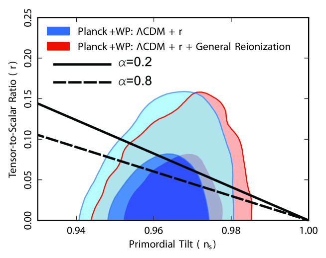
Figure 3: This plot shows the parameter $r$ as a function of the scalar spectral index $n_{s}$ for two values of the constant $\alpha$, i. e. $\alpha=0.2$ (solid line) and $\alpha=0.8$ (dashed line). The values of $r$ have been normalized in such a way that we have $r=0$ when $n_{s}=1$.

Finally, combining the expression for $n_{T}$ together with the expression for the $r$ parameter we get that $r=-\frac{1}{2}\,n_{T}$. This expression corresponds to the inflationary consistency conditionK94 . However, this relation could be violated in some casesH02 . Furthermore, this consistency condition is useful to understand how $r$ is connected to the evolution of the scalar inflaton field. It is not hard to show that the following relation holds

$$\frac{\triangle\,\phi}{m_{Pl}}=\frac{1}{4\,\sqrt{\pi}}\,\int_{0}^{N}\,\sqrt{r}\,dN,$$ (50)

relation known as the Lyth boundL97 . As a consequence this relation implies that an inflaton variation of the order of the Planck mass is needed to produce $r\geq 0.01$Planck2013 . By using the expression that we found for the $r$ parameter, expressed by Eq. (48), and using the result for the number of e-folds, $N$, expressed by Eq. (26), we get that

$$\frac{\triangle\,\phi}{m_{Pl}}=\frac{1}{4}\,\sqrt{\frac{6}{\pi}}\,\ln\left[\frac{e^{\frac{3}{2}N}+\sqrt{e^{3N}+1}}{1+\sqrt{2}}\right].$$ (51)

For instance, by taking some values of the number of e-folding we get that $\displaystyle\frac{\triangle\,\phi}{m_{Pl}}\approx 31$ and $\displaystyle\frac{\triangle\,\phi}{m_{Pl}}\approx 36$, for $N=60$ and $N=70$, respectively.

V conclusions

We have considered an inflationary universe model in which the inflaton field is characterized by an Equation of state corresponding to a generalized Chaplygin gas, i.e. $\displaystyle p_{\phi}=-\frac{B}{\rho_{\phi}^{\alpha}}$, where $\alpha$ is the generalized Chaplygin gas parameter, and was considered to lie in the range $0\leq\alpha\leq 1$. In this study it was described the kinematical evolution where the Hubble parameter was taken to be given by $\displaystyle H(\phi)=H_{0}\,\cosh^{\frac{1}{1+\alpha}}\,\left[\sqrt{\frac{6\,\pi}{m_{Pl}^{2}}}\,(1+\alpha)(\phi-\phi_{0})\right]$. Here, the scalar potential, the corresponding number of e-folding and the attractor feature of the model were described. We should mention here that the scalar potential related to the inflaton field results in such a way that it is possible to reproduce a generalized Chaplygin gas, requiring that some specific initial conditions on the inflaton field and its time derivative are chosen. Here, it was shown that this sort of potential works quite well when this is contrasted with the measurement recently released by the Planck data. This situation is the main motivation to study inflationary universe models with this kind of scalar potential.

Then, we determined the scalar and tensor spectrum indices in term of $\epsilon_{{}_{H}}$ and $\eta_{{}_{H}}$ parameters. From these quantities we were able to write down explicit expressions for the running scalar spectral index, $n_{run}$, and the tensor-to-scalar ratio, $r$, parameters.

The resulting contours in the $r-n_{s}$ plane were presented for two different values of the generalized Chaplygin gas parameter $\alpha=0.2$ and $\alpha=0.8$. In this plot we have confronted our results with recent data released by Planck, where marginalized joint $68\%$ and $95\%$ Confident Level regions for Planck plus WMAP data for the model $\Lambda$CDM plus $r$ were used. Also, by using the values released by Planck for the $n_{s}$ parameter and its running, $n_{run}$, was able to obtain a value for the $\alpha$ parameter given by the value $\alpha=0.2578\pm 0.0009$.

In general terms, we have found that the tensor-to-scalar ratio can adequately accommodate the currently available observational data for some values of the parameter $\alpha$. In this context, it seems that the model described here is appropriated for describing inflationary universe models.

- (1) A. Linde, Particle Physics and Inflationary Cosmology. Gordon and Breach, New York, USA, (1990).
- (2) WMAP Collaboration, H.V. Peiris et al., Astrophys. J. Suppl. 148, 213 (2003); WMAP collaboration, J. Dunkley et al., Astrophys. J. Suppl. 180, 306 (2009); WMAP collaboration, G. Hinshaw et al., Astrophys. J. Suppl. 180, 225 (2009); WMAP collaboration, M.R. Nolta et al., Astrophys. J. Suppl. 180, 296 (2009);WMAP collaboration, N. Jarozic et al., The Astrophys. J. Suppl. 192, 14 (2011); WMAP collaboration, E. Komatsu et al., Astrophys. J. Suppl. 192, 18 (2011).
- (3) P. A. R. Ade et al. [Planck Collaboration], arXiv:1303.5082 [astro-ph.CO].
- (4) J.E. Lisdey, Class. Quantum Grav. 8, 923 (1991).
- (5) L.P. Grishchuk and Y.V. Sidorav, in Fourth Seminar on Quantum Gravity, edited by M.A. Markov, V.A. Berezin, and V.P. Frolov (World Scientific, Singapore, 1988); A.G. Muslinov, Class. Quantum Grav. 7, 231 (1990); D.S. Salopek, J.R. Bond, and J.M. Bardeen, Phys. Rev. D 40, 1753 (1989).
- (6) J.E. Lidsey et al., Rev. Mod. Phys. 69, 373 (1997).
- (7) S. del Campo, JCAP 1212, 05 (2012).
- (8) N. Billic, G. B.Tupper and R. D. Viollier, Phys. Lett. B 535 17 (2001).
- (9) M. C. Bento, O. Bertolami and A. A. Sen, Phys. Rev. D 66 043507 (2002).
- (10) V. Gorini, A. Kamenschik and U. Moschella, Phys. Rev. D 67 063509 (2003).
- (11) M. C. Bento, O. Bertolami, and A. A. Sen, Phys. Rev. D, 70 083519 (2004).
- (12) A.Yu. Kamenshchik, U. Moschella and V. Pasquier, Phys. Lett. B 511 265 (2001).
- (13) F. Perrotta, S. Matarrese and M. Torki, Phys.Rev. D 70 121304 (2004).
- (14) V. Gorini, A. Kamenshchik, U. Moschella, V. Pasquier and A. Starobinsky, Phys. Rev. D 72 103518 (2005).
- (15) C. Uggla, Phys. Rev. D 88 064040 (2013).
- (16) N. Liang, L. Xu and Z.-H. Zhu, Astron. & Astrophys., 527 A11 (2011).
- (17) R. C. Freitas, S. V. B. Gonçalves and H. E. S. Velten, Phys. Lett. B, 703 209 (2011);
- (18) J. C. Fabris, C. Ogouyandjou, J. Tossa and H. E. S. Velten, Phys. lett. B, 694 289 (2011).
- (19) R. Lazkoz, A. Montiel and V. Salzano, Phys. Rev. D, 86 103535 (2012).
- (20) J. V. Cunha, J. S. Alcaniz and J. A. S. Lima, Phys. rev. D 69 083501 (2004).
- (21) V. Sahni, T. D. Saini and A. A. Starobinsky and U. Alam, JETP Lett. 77 201 (2003).
- (22) Y. Wang, D. Wands, L. Xu, J. De-Santiago and A. Hojjati, Phys. rev. D 87, 083503 (2013).
- (23) H. A. Borges, S. Carneiro, J. C. Fabris and W. Zimdahl, arXiv: 1306.0917v1[astro-ph.CO].
- (24) S. del Campo, et al, Phys. Rev. D, 88 , 023532 (2013).
- (25) R. Jackiw, A Particle field theorist’s lectures on supersymmetric, nonAbelian fluid mechanics and d-branes arXiv: physics-0010042; N. Ogawa, Phys. Rev. D 62, 085023 (2000); A. Kamenshchik et al., Phys. Lett. B 487, 7 (2000); N. Bilic, G. B. Tupper, R. D. Viollier, Phys. Lett., B 535, 17 (2002); J. C. Fabris, S. V. B. Goncalves, P. E. de Souza, Gen. Relativ. Grav. 34, 53 (2002).
- (26) M. Bouhmadi-López and P. Vargas Moniz, Phys. Rev. D 71, 063521 (2005); O. Bertolami and V. Duvvuri, Phys. Lett. B 640, 121 (2006); Bouhmadi-López, C. Kiefer, B. Sandhöfer and P. V. Moniz, Phys. Rev. D 79, 124035 (2009); M. Bouhmadi-López, P. Frazão and A. B. Henriques, Phys. Rev. D 81, 063504 (2010).
- (27) S. del Campo and R. Herrera, Phys. Lett. B, 660 282 (2008).
- (28) A. R. Liddle, P. Parson and J. D. Barrow, Phys. Rev. D 50, 7222 (1994).
- (29) D.S. Salopek and J.R. Bond, Phys. Rev. D 42, 3936 (1990).
- (30) V.F. Mukhanov and G.V. Chibisov, JETP Lett. 33, 532 (1981).
- (31) V.N. Lukash, Zh. Eksp. Teor. Fiz. (JETP) 79, 1601 (1980); S.W. Hawking, Phys. Lett. B 115, 295 (1982); A.A. Starobinsky, Phys. lett. B 117, 175 (1982).
- (32) L.P. Grishchuk, Sov. Phys. JETP 40, 409 (1975); A.A. Starobinsky, JETP Lett. 30, 682 (1979); V. Rubakov, M. Sazhin, and A. Veryaskin, Phys. Lett. B 115, 189 (1982); R. Fabbri and M.D. Pollock, Phys. Lett. B 125, 445 (1983); L. Abbott and M. Wise, Nucl. Phys. B 244, 541 (1984).
- (33) For a review see V. F. Mukhanov, H. Feldman, and R. H. Brandenberger, Phys. Rept. 215, 203 (1992). See also V.N. Lukash, VIII Brazilian School of Cosmology and Gravitation II, edited by M. Novello. (Editions Frontiers, Rio de Janeiro, Brazil, 1995).
- (34) M. Kamionkowski, A. Kosowski and A. Stebbins, Phys. Rev. Lett. 78, 2058 (1997); L. Knox and Y. Song, Phys. Rev. Lett. 89, 011303 (2002).
- (35) G. B. Field and L. C. Shepley, Astrophys. Space. Sci. 1 , 309 (1968); V. N. Lukash, Sov. Phys. JETP 52, 807 (1980); Sov. Phys. JETP Lett. 31, 596 (1980); G. V. Chibisov and V. F. Mukanov, Mon. Not. R. Astron. Soc. 200, 535 (1982); V.F. Mukanov, Sov. Phys. JEPT Lett. 41, 493 (1985); M. Sasaki, Prog. Theor. Phys. 76, 1036 (1986); Sov. Phys. JETP 68, 1297 (1988); V.F. Mukanov, Fisical Foundations of Cosmology (Cambridge University Press, Cambridge, 2005).
- (36) J.M. Barneer, P.J. Steinhardt and M.S. Turner, Phys. Rev. D 28, 679 (1983).
- (37) E. D. Stewart and D. H. Lyth, Phys. Lett. B 302, 171 (1993).
- (38) D. H. Lyth and E. D. Stewart, Phys. Lett. B 274, 168 (1992).
- (39) W.H. Kinney, Phys. Rev. D 56, 2002 (1997).
- (40) Other initial conditions have been impossed, for instance coherent states. See S. Kundu, J. Cosmol. Astropart. Phys. 1202 (2012) 005 for more details.
- (41) A. Guth and S.-Y. Pi, Phys. Rev. Lett. 49, 1110 (1982); J.M. Bardeen, P.J. Steinhardt and M.S. Turner, Phys. Rev. D 28 679 (1983).
- (42) S. Hawking, Phys. Lett. B 115 295 (1982).
- (43) E.W. Kolb and S.L. Vadas, Phys. Rev. D 50, 2479 (1994).
- (44) L. Hui and W.H. Kinney, Phys. Rev. D 65, 103507 (2002).
- (45) D. H. Lyth, Phys. Rev. Lett., 78, 1861 (1997).