High-loop perturbative renormalization constants
for Lattice QCD (II):
three-loop quark currents for tree-level Symanzik improved gauge action and $n_{f}=2$ Wilson fermions

Abstract

Numerical Stochastic Perturbation Theory was able to get three- (and even four-) loop results for finite Lattice QCD renormalization constants. More recently, a conceptual and technical framework has been devised to tame finite size effects, which had been reported to be significant for (logarithmically) divergent renormalization constants. In this work we present three-loop results for fermion bilinears in the Lattice QCD regularization defined by tree-level Symanzik improved gauge action and $n_{f}=2$ Wilson fermions. We discuss both finite and divergent renormalization constants in the RI’-MOM scheme. Since renormalization conditions are defined in the chiral limit, our results also apply to Twisted Mass QCD, for which non-perturbative computations of the same quantities are available.
We emphasize the importance of carefully accounting for both finite lattice space and finite volume effects. In our opinion the latter have in general not attracted the attention they would deserve.

1 Introduction

A few years ago the Parma group embarked in an ambitious program: computing renormalization constants for lattice QCD to three-loop accuracy. Since a non-perturbative computation of renormalization constants (RCs) has been the preferred choice for quite a long time, the rationale for such a program deserves a few words. The theoretical status of a perturbative computation of RCs is in principle firm: from a fundamental point of view, renormalizability is strictly speaking proved only in Perturbation Theory (PT) and quantities like fermion bilinears are either finite or only logarithmically divergent; since there are no power divergences, PT must work. From a practical point of view difficulties show up: traditional (diagrammatic) Lattice PT is cumbersome, so that one can get at most two-loop results; in practice, most results are only one-loop. Since Lattice PT itself is badly convergent, this is a serious concern. Numerical Stochastic Perturbation Theory (NSPT [1, 2]) enables high-loop computations and circumvents this problem. Indeed, three- (and even four-) loop results were published for finite RCs in the scheme defined by Wilson action and Wilson fermions [3].

A follow-up of [3] was announced for logarithmically divergent currents, for which a careful assessment of finite size effects is needed. In recent years a clean way to effectively control the latter was introduced in [4, 5], which we put at work also here. This is the first of two papers dealing with the three-loop computation of Lattice QCD RCs in the RI’-MOM scheme for plain Wilson fermions and improved gauge actions: in the present paper we report results for the tree-level Symanzik improved gauge action with $n_{f}=2$ and discuss the general framework of finite lattice spacing and finite size corrections; in a second one we deal with Iwasaki gauge action with $n_{f}=4$ and tackle the all the problems connected with summing PT series for Lattice QCD RCs [6]. Updates on these computations have been presented in recent years at the Lattice conferences, and in particular preliminary results were quoted in [7]. We emphasize that in both cases ($n_{f}=2$ tree-level Symanzik and $n_{f}=4$ Iwasaki) results can be compared with analogous non-perturbative computations for Twisted Mass fermions [8, 9]: since the renormalization scheme is massless, RCs are the same. In another paper we will finally fill the gap which was left in [3] for RCs of logarithmically divergent currents for Wilson fermions and Wilson gauge action.

The overall structure of this paper is as follows:

• RI’-MOM is the scheme we adhere to. Section 2 recalls the basic definitions and points out a crucial issue for the success of our computations: the logarithmic contributions to the RCs we will compute can be got from continuum computations which are available in the literature.

• From the discussion of Section 2 it will be clear that a two-loop matching of continuum and lattice scheme is needed. Since this is not available in the literature for the gauge action at hand (tree-level Symanzik), we derive it in Section 3. We comment on the level of accuracy which we can attain, discuss in which sense this is enough and put forward the strategy for a better determination.

• No chiral extrapolation is needed in our computations. In PT staying at zero quark mass is enforced by inserting the proper counterterms: in Section 4 we present our three-loop result for the Wilson fermions critical mass for the tree-level Symanzik action (with $n_{f}=2$). This section also contains a few technical details on our computations (e.g. the number of configurations which were generated).

• The extraction of the continuum limit is attained by fitting irrelevant contributions, which should be compliant to the lattice symmetries. This should be done having in mind that RI’-MOM is defined in the infinite volume: there is a subtle interplay between fitting finite lattice spacing and finite volume corrections. Section 5 is devoted to a general discussion of our strategy to get results in the continuum and in the infinite volume limit.

• Section 6 contains our results; in particular, we briefly comment on the comparison with non-perturbative results.

As said, this paper has a follow-up in [6], which contains more remarks on different ways of summing the series, trying to single out the different (relevant and irrelevant) contributions. In [6] we also comment to which extent the techniques we put at work in the NSPT context can provide a fresher look into the lattice version of the RI’-MOM scheme.

2 RI’-MOM and its logarithms

RI’-MOM is one of the most popular renormalization schemes for Lattice QCD [11]; being regulator independent, it can be effectively adopted in a lattice regularization. While this has been highly recognized, one technical detail has been not yet fully appreciated: in a RI’-MOM perturbative computation of lattice RCs, logarithmic contributions can be inferred from continuum computations. This is extremely useful to us. In a traditional computation, logarithmic contributions are the easy part, while finite terms require the really big efforts; in NSPT it is just the other way around. As it will be clear in the following, we need to fit our results to single out relevant and irrelevant contributions. While disentangling logarithmic and finite terms is in principle feasible, this would require a terrific numerical precision, de facto impossible to attain.

To renormalize quark bilinears in RI’-MOM one starts from Green functions constructed as expectation values computed on external quark states at fixed momentum $p$

$$G_{\Gamma}(p)\,=\,\int dx\,\langle p|\;\overline{\psi}(x)\Gamma\psi(x)\;|p\rangle$$

By inserting different $\Gamma$ one obtains the Green functions relevant for the different currents, e.g. the scalar (identity), pseudoscalar ($\gamma_{5}$), vector ($\gamma_{\mu}$), axial ($\gamma_{5}\gamma_{\mu}$). Since these are gauge-dependent quantities, a choice for the gauge has to be made. As it is common for the lattice implementation of RI’-MOM, Landau gauge is our choice. This is mainly due to technical reasons, since Landau gauge can be enforced in a lattice simulation by a minimization procedure. For NSPT the same holds, including the additional choice of Fast Fourier Transform acceleration (see [1, 2]). From Green functions, vertex functions are then obtained by amputation ($S(p)$ is the quark propagator)

$$\Gamma_{\Gamma}(p)=S^{-1}(p)\,G_{\Gamma}(p)\,S^{-1}(p).$$

The quark field renormalization constant has to be computed from the condition

$$Z_{q}(\mu,\alpha)=-i{{1}\over{12}}{{Tr(\not{p}S^{-1}(p))}\over{p^{2}}}|_{p^{2}=\mu^{2}}.$$ (1)

After projecting on tree-level structure

$$O_{\Gamma}(p)=Tr\left(\hat{P}_{O_{\Gamma}}\Gamma_{\Gamma}(p)\right),$$ (2)

one enforces renormalization conditions that read

$$Z_{O_{\Gamma}}(\mu,\alpha)Z_{q}^{-1}(\mu,\alpha)O_{\Gamma}(p)|_{p^{2}=\mu^{2}}=1.$$ (3)

In order to have a mass-independent scheme, all this is defined at zero quark mass.

In a lattice perturbative computation, we can write the generic $Z$ in the continuum limit ($a\rightarrow 0$)

$$Z(\mu,\alpha)=1+\sum_{n>0}d_{n}({l})\,\alpha(\mu)^{n}\qquad d_{n}({l})=\sum_{i=0}^{n}d_{n}^{(i)}{l}^{i}\qquad{l}\equiv\log(\mu a)^{2}$$ (4)

where the lattice cutoff ($a$) is in place and the expansion is in the renormalized coupling. To make our notations a bit lighter, we have omitted any reference to any operator, i.e. we wrote $Z$ and not $Z_{O_{\Gamma}}$ as we did a few lines above. In the same spirit we have omitted any dependence on the (covariant) gauge parameter $\lambda$: as already pointed out, the reader has to assume the choice $\lambda=0$ (Landau). Making this choice explicit simplifies the formulas; we will comment on the general formulation a few lines below, pointing out why our (apparently naive) notation is indeed correct for Landau gauge. For finite quantities (e.g. vector and axial currents) $d_{n}^{(i>0)}=0$; for divergent quantities (e.g. scalar and pseudoscalar currents) divergencies show up as powers of $\log(\mu a)^{2}$. To compute the $Z$s in NSPT, we want to eventually manage expansions in the bare lattice coupling $\alpha_{0}$

$$Z(\mu,\alpha_{0})=1+\sum_{n>0}\overline{d}_{n}({l})\,\alpha_{0}^{n}\qquad\overline{d}_{n}({l})=\sum_{i=0}^{n}\overline{d}_{n}^{(i)}{l}^{i}.$$ (5)

By differentiating Eq. (4) with respect to $\log(\mu a)^{2}$ one obtains the expression for the anomalous dimension

$$\gamma={{1}\over{2}}{{d}\over{d{l}}}\log Z.$$

Since this is a scheme dependent, finite quantity, one has to recover an expansion in which coefficients are finite numbers (with no dependence on the regulator left)

$$\gamma=\sum_{n>0}\gamma_{n}\,\,\alpha(\mu)^{n}.$$ (6)

This expansion is known to three-loop accuracy from continuum computations [12]. Imposing that the expression obtained by differentiating Eq. (4) matches Eq. (6) (with the proper values for the $\gamma_{n}$ read from [12]) we can obtain the expressions of all the $d_{n}^{(i>0)}\,(n\leq 3)$. In practice the solution comes from the request that all the (powers of the) logarithms cancel out; as a result, each $d_{n}^{(i>0)}$ is expressed in terms of the $\gamma_{m\leq n}$, the $d_{m\leq n}^{(0)}$ and the coefficients of the $\beta$-function; the latter come into place since part of the dependence on $\mu$ in Eq. (4) is via the coupling $\alpha(\mu)$.

The $\overline{d}_{n}^{(i>0)}$ of Eq. (5) can finally be obtained by re-expressing the expansion in Eq. (4) as an expansion in the bare coupling $\alpha_{0}$. This makes the $\overline{d}_{n}^{(i)}$ depend (also) on the coefficients of the matching of the continuum and the lattice couplings. In particular, our three-loop expansion of the Zs asks for a two-loop matching of the continuum coupling to the lattice coupling in the scheme we are working in, i.e. tree-level Symanzik gauge action with $n_{f}=2$ Wilson fermions. Since this is not known from the literature ([13] provides a one-loop matching), we derived it: this is discussed in the next section.

We now come back to the issue of (covariant) gauge parameter dependence. In a generic (covariant) gauge, not only the dependence on $\lambda$ enters Eq. (4), but also the gauge parameter anomalous dimension comes into place in linking Eq. (4) to Eq. (6). We have worked out the formulas with generic $\lambda$ and checked the correctness of our results with the two-loop computations of [14], which are obtained in Feynman gauge. Notice that the apparently naive recipe of neglecting the $\lambda$-dependence from the very beginning (as we did in our previous discussion) returns correct results, i.e. one obtains the same results by keeping track of all the $\lambda$-dependences and by finally putting $\lambda=0$. This is due to the fact that the non trivial dependence on the gauge parameter anomalous dimension is itself proportional to $\lambda$.

The expressions for the $\overline{d}_{n}^{(i>0)}$ (and $d_{n}^{(i>0)}$) are available upon request in the form of Mathematica notebooks; in the following we will focus on the finite $\overline{d}_{n}^{(0)}\,(n\leq 3)$ and adhere to the standard recipe of summing the series at $\mu a=1$. Actually we will report the results as expansions in yet another coupling, namely $\beta^{-1}\equiv{{2\pi\alpha_{0}}\over{3}}$ (more on this later). As we have already pointed out, in order to reconstruct the whole set $\{\overline{d}_{n}^{(i>0)}\}$, the only piece of information which is missing in the literature is the two-loop matching of continuum to lattice coupling for the regularization at hand: we report this result in the next section.

3 Two-loop matching of continuum and lattice couplings

In the following we provide the matching of couplings enabling us to go from Eq. (4) to Eq. (5). We will make use of the notation $\alpha_{0}=\alpha_{TLS}$ to enlighten that the lattice coupling we are referring to is the one defined by the regularization at hand, with the Tree-Level Symanzik (TLS) gauge action in place. The matching will be to the $\overline{MS}$ scheme, $\alpha_{\overline{MS}}$ being the coupling in which the expansions in [12] are expressed (strictly speaking, it suffices that this holds at the finite order one is interested in).

The general form of the matching between two schemes (unprimed and primed) reads

$$\alpha(s\mu)=\alpha^{\prime}(\mu)+c_{1}(s)\,\alpha^{\prime}(\mu)^{2}+c_{2}(s)\,\alpha^{\prime}(\mu)^{3}+\ldots.$$ (7)

The coefficient $s$ accounts for the choice of different momentum scales; it enters the expressions for the matching coefficients $c_{1}(s)$ and $c_{2}(s)$

$$c_{1}(s) = 2b_{0}\log{{\Lambda}\over{\Lambda^{\prime}}}-2b_{0}\log{s}$$ (8)

$$c_{2}(s) = c_{1}(s)^{2}-2b_{1}\log{s}+2b_{1}\log{{\Lambda}\over{\Lambda^{\prime}}}+{{b_{2}-b_{2}^{\prime}}\over{b_{0}}}.$$ (9)

Here $b_{0},b_{1},b_{2}$ and $b_{2}^{\prime}$ are coefficients of the $\beta$-function, while $\Lambda$ and $\Lambda^{\prime}$ are the scales associated with the two regularizations. While $b_{0}$ and $b_{1}$ are universal, $\Lambda$ and $b_{2}$ depend on the scheme (and so they come in both primed and unprimed versions). Notice that Eq. (9) states that the two loop matching of $\alpha_{TLS}$ to $\alpha_{\overline{MS}}$ also entails the knowledge of $b_{2}^{TLS}$, since $b_{2}^{\overline{MS}}$ is known.

3.1 Strategy for the matching

There is no obvious way of computing the direct matching of $\overline{MS}$ to the TLS scheme making use of NSPT. We will go through the strategy of first matching to an intermediate scheme. Once again, we will rely on the fact that no computation of logarithms will be needed: every relevant logarithmic dependence is known. The strategy has already been used in [15, 16] (although in those works we had another goal).

In the lattice regularization defined by TLS gauge action and $n_{f}=2$ Wilson fermions, we computed the perturbative expansions of rectangular Wilson loops $W(R,T)$ (of extensions $R$ and $T$) and from those we computed logarithms of Creutz ratios

$$V_{T}(R)=\log\left({{W(R,T-1)}\over{W(T,R)}}\right).$$

Notice that in the previous formula everything is dimensionless. In particular, $R$ and $T$ are measured in lattice units (i.e. they are integer numbers): at a given, fixed value of the lattice spacing $a$, physical lengths associated to them are $r=Ra,\,t=Ta$. The static quark potential can be defined via

$$aV(r)=aV(Ra)=\lim_{T\to\infty}V_{T}(R).$$

The static quark potential is the quantity which describes the interaction energy of a infinitely heavy $q\bar{q}$ pair at a distance $r$, which in its full (non-perturbative) form is in first approximation just the sum of a string tension contribution, which is responsible for confinement, and a $r^{-1}$ contribution, whose interpretation is different in different IR/UV regimes

$$V(r)={{C}\over{r}}+\sigma r.$$

In PT the first term is just the Coulomb potential and there is no string tension. In a lattice regularization, one is left in addition with a linearly divergent term, which gives the so called residual mass of the heavy quark:

$$aV(r)=aV(Ra)=2\delta m-C_{F}{{\alpha_{V}(r^{-1})}\over{R}}.$$ (10)

While $\delta m$ is associated to a linearly divergent quantity, logarithmic divergencies are absorbed in $\alpha_{V}$; extra (corners) divergences are absent because the quantity is built out of ratio of rectangular loops. Eq. (10) defines the potential coupling $\alpha_{V}(r^{-1})$ we will be concerned with. Notice that the perturbative computation of the (power divergent) residual mass is not supposed to be a reliable one.

A perturbative computation of the static quark potential in our lattice scheme reads

$$aV(r)=aV(Ra) = V_{0}(R)\,\alpha_{TLS}+V_{1}(R)\,\alpha_{TLS}^{2}+V_{2}(R)\,\alpha_{TLS}^{3}+\mathcal{O}(\alpha_{TLS}^{4})$$

$$= 2\left(\delta m_{0}\,\alpha_{TLS}+\delta m_{1}\,\alpha_{TLS}^{2}+\delta m_{2}\,\alpha_{TLS}^{3}+\mathcal{O}(\alpha_{TLS}^{4})\right)+$$

$$-C_{F}{{\alpha_{TLS}}\over{R}}\left(1+C_{1}(R)\,\alpha_{TLS}+C_{2}(R)\,\alpha_{TLS}^{2}+\mathcal{O}(\alpha_{TLS}^{3})\right),$$

where subscripts are written according to the actual loop counting.

In order to trade the description in terms of the $V_{i}(R)$ for that in terms of $\delta m_{i}$ and $C_{i}(R)$ one has to disentangle constant and $R^{-1}$ contributions: in NSPT this requires a fitting procedure. The description in terms of $\delta m_{i}$ and $C_{i}(R)$ is the order by order version of Eq. (10): we have actually computed $\alpha_{V}(r^{-1})$ as an expansion

$$\alpha_{V}(r^{-1})=\alpha_{TLS}+C_{1}(R)\,\alpha_{TLS}^{2}+C_{2}(R)\,\alpha_{TLS}^{3}+\mathcal{O}(\alpha_{TLS}^{4}).$$ (12)

To be more precise, this is simply a particular case of the matching (7): it is the matching of the continuum coupling $\alpha_{V}(r^{-1})$ to the lattice coupling $\alpha_{TLS}$. Since the latter is defined at the scale $a^{-1}$ while $\alpha_{V}(r^{-1})$ is defined at the scale $r^{-1}=a^{-1}R^{-1}$, the factor $s$ of Eq. (7) here reads $s=R^{-1}$. In other words, we can read the $C_{i}(R)$ from Eq. (8) and Eq. (9) (i.e. $C_{i}(R)=c_{i}(R^{-1})$)

$$C_{1}(R) = 2b_{0}\log{{\Lambda_{V}}\over{\Lambda_{TLS}}}+2b_{0}\log{R}$$ (13)

$$C_{2}(R) = C_{1}(R)^{2}+2b_{1}\log{R}+2b_{1}\log{{\Lambda_{V}}\over{\Lambda_{TLS}}}+{{b_{2}^{(V)}-b_{2}^{(TLS)}}\over{b_{0}}}.$$ (14)

Notice that everything has been written in the limit $a\rightarrow 0$ (and in the infinite volume limit, as it is clear from the definition of $aV(Ra)$ in terms of $V_{T}(R)$). We will have to come back to this when we discuss the NSPT computation.

As a byproduct of our computation we also obtain the residual mass $\delta m$ as an expansion in $\alpha_{TLS}$

$$\sum_{n\geq 0}\delta m_{n}\,\alpha_{TLS}^{n+1}.$$ (15)

Once we have computed the matching between $\alpha_{V}(R)$ and $\alpha_{TLS}$, we need the matching of $\alpha_{V}(R)$ to $\alpha_{\overline{MS}}$. This can be read from the computation in [17].

3.2 Results

The NSPT computations were performed on a $32^{4}$ lattice; we computed the Wilson loops $W(R,T)$ for all the values of $R$ and $T$ up to 16. The quark mass was set to zero by plugging the appropriate mass counterterm, i.e. the perturbative critical mass as read from [19] (see next Section). Results were averaged over $\sim$150 lattice configurations.

From the $W(R,T)$ we computed the $V_{T}(R)$. We could not take the $T\to\infty$ limit, but regarded the $V_{T}(R)$ as our estimate for $aV(Ra)$. This is a first (finite volume) approximation in our setting. By fitting (order-by-order) our $V_{T}(R)$ data to $aV(Ra)$ as defined by eq. (3.1) (which is valid in the $a\rightarrow 0$ limit) we incurred yet another source of approximation, since no attempt was made to take into account irrelevant, finite $a$ effects. Despite the distortions expected from these lattice artifacts, we extracted from our data both the residual quark mass $\delta m_{i}$ and the expected $C_{i}(R)$ (i.e. we fitted the parameters entering their expressions). Since most of the parameters are known, we can estimate a posteriori how good (or bad) the procedure is.

In order to at least minimize the irrelevant effects we considered intervals of $R$ such that

• $T>R$ ($T/R\sim 2.5$);

• $R$ itself is not too small ($R\geq 3$);

• the fitting intervals themselves are from 3 up to 7 points long.

On top of the systematic (lattice artifacts) errors, results are of course also affected by statistical errors. The relative weight of these effects is different for different orders. This actually opens the way to a possible (careful) tradeoff between the errors. We adopted the following strategy: when systematic effects are clearly distinguishable (i.e. statistical effects are relatively small), we only considered $T=16$ data (this is the case of the tree-level potential). When statistical errors are significant on their own, the systematic (finite $T$) effect is not that clear. In this case we decided to neglect this systematic effect and tame the statistical noise by averaging over different values of $T$ (from $T=14$ to $T=16$). In this way we obtained smoother curves. Further details can be found in [18].

In order to verify the reliability of our approach we first checked known results. Notice that despite the coupling parameters are known, even lower order results are not trivial, since at any order residual mass is unknown (we got it as a byproduct). In Figure 1 we show our estimates for tree-level, one-loop and two-loop potential. We estimated $3\leq R\leq 7$ as the best fitting interval for tree-level and one loop; the same interval was also taken for two-loop computation.

Tree-level data were fitted to the functional form

$$V_{0}(R)=2\delta m_{0}-{{C_{F}}\over{R}}$$

obtaining $\delta m_{0}=1.84\pm 0.01$, while $C_{F}$ is reconstructed to a few percent. This gives a first rough idea of the impact of systematic effects.

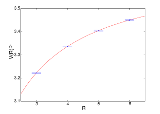
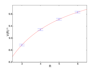
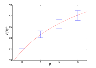
Figure 1: Data and fit (continuous line) for (from left to right) tree-level, one-loop, two-loop potential.

At one-loop, we plugged the analytical value for $C_{F}$ and tried to fit the constant term $\log{{\Lambda_{V}}\over{\Lambda_{(TLS)}}}$ in the functional form

$$V_{1}(R)=\delta m_{1}-{{C_{F}}\over{R}}2b_{0}\left(\log R+\log{{\Lambda_{V}}\over{\Lambda_{TLS}}}\right).$$

We obtained $\log{{\Lambda_{V}}\over{\Lambda_{(TLS)}}}=2.8\pm 0.1$, to be compared to the analytical result $2.8191$ [13]. We also obtained $\delta m_{1}=5.71\pm 0.01$.

At two-loop we finally tackled the determination of the quantity we are interested in; the functional form

$$V_{2}(R)=\delta m_{2}-{{C_{F}}\over{R}}\left(c_{1}(R)^{2}+2b_{1}\log R+2b_{1}\log{{\Lambda_{V}}\over{\Lambda_{TLS}}}+{{b_{2}^{(V)}-b_{2}^{(TLS)}}\over{b_{0}}}\right).$$

depends on the unknown $\delta m_{2}$ and ${{b_{2}^{(V)}-b_{2}^{(TLS)}}\over{b_{0}}}$. As one can see from the figure, at two-loop fluctuations are larger than at lower orders, and as a consequence the fit suffers from a larger indetermination. In this case we obtained $\delta m_{2}=30\pm 1$ and

$${{b_{2}^{(V)}-b_{2}^{(TLS)}}\over{b_{0}}}\equiv X=4\pm 1$$

where we have introduced a notation ($X$) we will make use of later. Though the relative error in this value is high, we must emphasize that one is interested in the final matching to $\alpha_{\overline{MS}}$. From [17] we can get the matching of $\alpha_{V}$ to $\alpha_{\overline{MS}}$, and the final result is (remember that this holds for $n_{f}=2$, with Wilson regularization for the lattice fermions)

$$\alpha_{\overline{MS}}=\alpha_{TLS}+2.79866\,\alpha_{TLS}^{2}+(11.5\pm 1.0)\,\alpha_{TLS}^{3}+\mathcal{O}(\alpha_{TLS}^{4}),$$

where the relative error on the second coefficient is slightly less than 10%.

Notice that in order to assess the effectiveness of our computation, this is not yet the end of the story. What we are really interested in is how the parameter $X$ (which fixes this matching) enters the coefficient $\overline{d}_{3}^{(1)}$ of Eq. (5). Actually in the following we will report our results as expansions in the lattice coupling $\beta^{-1}$ (we specify the definition to the case at hand, i.e. SU(3))

$$\beta^{-1}\equiv{{g_{0}^{2}}\over{6}}\equiv{{2\pi\alpha_{0}}\over{3}}$$

$$Z(\mu,\beta^{-1})=1+\sum_{n>0}z_{n}({l})\,\beta^{-n}\qquad z_{n}({l})=\sum_{i=0}^{n}z_{n}^{(i)}{l}^{i}\qquad{l}\equiv\log(\mu a)^{2}$$ (16)

We now show how the parameter $X$ enters $z_{S\,3}^{(1)}$, where the extra subscript $S$ indicates that we are taking the example of the renormalization of the scalar current:

$$z_{S\,3}^{(1)}=1.7823+0.0693\,X+0.7366\,z_{S\,1}^{(0)}+0.3040\,z_{S\,2}^{(0)}$$

This is the coefficient in front of the simple log in the three-loop order of the renormalization constant of the scalar current; a similar relation is in place for the pseudoscalar current. Apart from $X$, the only parameters in the formula are $z_{n<3}^{(0)}$ (all other numerics have been worked out explicitly): $z_{S\,1}^{(0)}=-0.6893$ is known analytically ([13]), while at two-loop we got $z_{S\,2}^{(0)}=-0.777(24)$. We can conclude the indetermination which is carried by $X$ is acceptable (namely, less than $10\%$). For the pseudoscalar current numerics is less favorable, but the indetermination remains acceptable (namely, of order $10\%$).

One could wonder whether NSPT can do better that what we showed in computing lattice to continuum coupling matchings. The answer is yes, a natural candidate for a more effective intermediate scheme being a finite volume one, e.g. the SF (Schroedinger Functional) scheme. A robust NSPT formulation of PT for the SF has been set up recently [20].

4 The three-loop critical mass

For Wilson fermions staying at zero quark mass amounts to the knowledge of the critical mass. In perturbation theory the latter has to be computed at the convenient order and plugged in as a counterterm: one does not need to go through an extrapolation process to reach the chiral limit (which can be a heavy task in a non-perturbative computation, in the end always acting as a source of systematic error).

In order to compute three-loop renormalization constants the effect of the critical mass has to be corrected up to two-loop order. Though it is not relevant for the computation at hand, we get as a by-product the value of the three-loop critical mass (which is a new result).

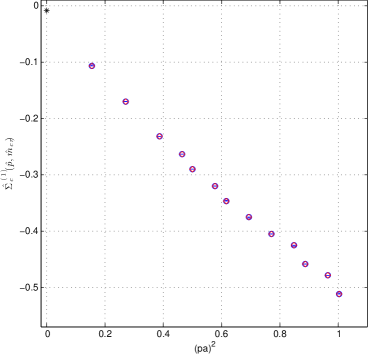
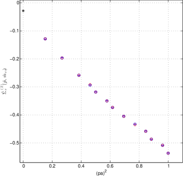
Figure 2: One-(left) and two-(right)loop $\hat{\Sigma_{c}}(\hat{p},\hat{m}_{cr},\beta^{-1})$ on a $32^{4}$ lattice: the (extrapolated) one- and two-loop values at $\hat{p}=0$ should be zero, because of counterterms, but they are not, because of finite volume.

The critical mass is computed from the inverse quark propagator

$$a\Gamma_{2}(\hat{p},\hat{m}_{cr},\beta^{-1})=aS(\hat{p},\hat{m}_{cr},\beta^{-1})^{-1}=i\hat{\not{p}}+\hat{m}_{W}(\hat{p})-\hat{\Sigma}(\hat{p},\hat{m}_{cr},\beta^{-1}).$$ (17)

In order to have less factors $a$ in place, we have here introduced a hat notation to denote dimensionless quantities (e.g. $\hat{p}=pa$): explicit factor of $a$ will be later singled out if needed. As already pointed out, $\beta^{-1}$ is the expansion parameter we adopt (and hence the dependence we quote). $\hat{m}_{W}(\hat{p})={\cal O}(\hat{p}^{2})$ is the (irrelevant) mass term generated at tree level by the Wilson prescription.

The dimensionless self-energy $\hat{\Sigma}(\hat{p},\hat{m}_{cr},\beta^{-1})$ (which is ${\cal O}(\beta^{-1})$) reads

$$\hat{\Sigma}(\hat{p},\hat{m}_{cr},\beta^{-1})=\hat{\Sigma}_{c}(\hat{p},\hat{m}_{cr},\beta^{-1})+\hat{\Sigma}_{\gamma}(\hat{p},\hat{m}_{cr},\beta^{-1})+\hat{\Sigma}_{\rm other}(\hat{p},\hat{m}_{cr},\beta^{-1}),$$ (18)

where we have singled out the component along the (Dirac space) identity

$$\hat{\Sigma}_{c}(\hat{p},\hat{m}_{cr})=1/4{\rm Tr_{spin}}(\hat{\Sigma}),$$

and the one along the gamma matrices

$${{1}\over{4}}\sum_{\mu}\gamma_{\mu}{\rm Tr_{spin}}(\gamma_{\mu}\hat{\Sigma})=\hat{\Sigma}_{\gamma},$$

while $\hat{\Sigma}_{\rm other}$ includes all other possible contributions along the remaining elements of the Dirac basis: these quantities are irrelevant and are always neglected in our analysis. The critical mass can be read from $\hat{\Sigma}_{c}$ at zero momentum

$$\hat{\Sigma}(0,\hat{m}_{cr},\beta^{-1})=\hat{\Sigma}_{c}(0,\hat{m}_{cr},\beta^{-1})=\,\hat{m}_{cr}.$$ (19)

Notice that restoring physical dimensions one recognizes that the critical mass is order $a^{-1}$, and so it must be cured by an additive counterterm. Since 1-loop and 2-loop orders are known [19], we plug their values as counterterms in our computations. As a result, a plot of one- and two-loop $\hat{\Sigma}_{c}$ vs momentum should display a zero intercept in zero. Actually this is not strictly speaking correct; on finite lattices one inspect corrections (which get smaller and smaller as the lattice size increases): see Fig. 2 for $32^{4}$ measurements.

The $p=0$ intercept of $\hat{\Sigma_{c}}(\hat{p},\hat{m}_{cr},\beta^{-1})$) comes from a fitting procedure: this is a general feature of our computations, as it will be clear in the next section. Since we want to remove the finite size effects, we perform our computations on different lattice sizes.

4.1 Data sets

Measurements were taken on different sizes: $32^{4}$, $20^{4}$, $16^{4}$, $12^{4}$. NSPT prescribes the numerical (order by order) integration of the Langevin equation (see [1, 2]). In this work we adopt the simplest numerical scheme, i.e. Euler scheme. To remove the effects of the finite time step $\epsilon$ an extrapolation $\epsilon\rightarrow 0$ (in this scheme a linear one) is needed. In view of this, measurements were taken on configurations generated at different values of $\epsilon$. Table 1 summarizes our statistics. The procedure is pretty the same as for non-perturbative simulations: configurations are generated on which one can later measure different observables. A preliminary analysis of the autocorrelations in place guided our choice for the frequency at which we save configurations. Residual autocorrelation effects are of course later accounted for in the analysis of different observables.
One should keep in mind that lattice sizes are actually pure numbers $N=L/a$: the coupling is in NSPT an expansion parameter and there is no physical value (say, in fermi) of the lattice spacing (and henceforth of the lattice size).

Table 1: Number of measurements at different value of the time step for the different lattice sizes.

lattice size $N=L/a$	$\epsilon=0.005$	$\epsilon=0.010$	$\epsilon=0.015$
$12$	118	115	119
$16$	195	136	184
$20$	20	31	41
$32$	22	19	22

4.2 Results

For each value of the lattice size and at each order in the coupling, we get the zero momentum value of $\hat{\Sigma_{c}}(\hat{p},\hat{m}_{cr},\beta^{-1})$) by fitting the latter as an expansion in hypercubic invariants, e.g.

$$\sum_{\nu}\hat{p}_{\nu}^{2}\;\;\;\;\;\;\;{{\sum_{\nu}\hat{p}_{\nu}^{4}}\over{\sum_{\nu}\hat{p}_{\nu}^{2}}}\;\;\;\;\;\;\;{(\sum_{\nu}\hat{p}_{\nu}^{2})}^{2}\;\;\;\;\;\;\;\sum_{\nu}\hat{p}_{\nu}^{4}\;\;\;\;\;\;\;{{\sum_{\nu}\hat{p}_{\nu}^{6}}\over{\sum_{\nu}\hat{p}_{\nu}^{2}}}\;\;\;\;\;\;\;\ldots$$ (20)

Figure 2 gives an idea of the effectiveness of such fits. Once we have the $\hat{\Sigma_{c}}(0,\hat{m}_{cr},\beta^{-1})$ for each lattice size, we have to extrapolate them to the infinite volume limit: Figure 3 displays the behavior of (one- and two-loop) results as inverse powers of $N=L/a$. Results are fully consistent with the (known) critical mass analytical values we have plugged in.

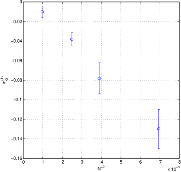
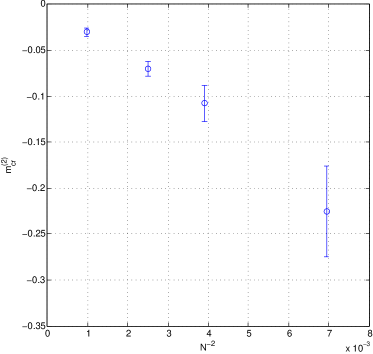
Figure 3: Infinite volume extrapolations of the one-(left) and two-(right)loop critical mass; data are plotted (and extrapolated) as functions of an inverse power of the lattice size $N=L/a$.

Things are different at three-loop order. Since the critical mass counterterm has been inserted up to two-loop order, $\hat{\Sigma_{c}}(\hat{p},\hat{m}_{cr},\beta^{-1})$ does not have to extrapolate to zero. We get instead a first original result: as a byproduct of our computations, we can estimate the three-loop critical mass. Three-loop results are plotted in Figure 4. The infinite volume extrapolation of our results reads $\hat{m}_{cr}^{(3)}=-3.94(4)$.

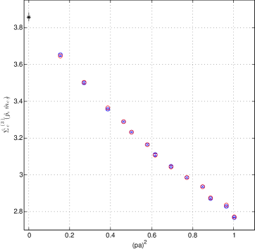
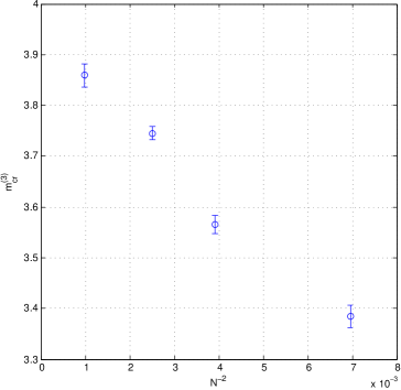
Figure 4: Three-loop critical mass: zero momentum extrapolation on a $32^{4}$ lattice (left) and infinite volume extrapolation (right).

5 The continuum and infinite volume limits of the $Z_{O_{\Gamma}}$

Our main goal is to compute the renormalization constants from our master formula Eq. (3). As said, in the $\beta^{-1}$ expansions of Eq.(16) the only unknown are the $z_{n}^{(0)}$: these are the quantities we are interested in. The $O_{\Gamma}(p)$ of Eq. (2) are the basic building blocks we have to compute; more precisely, we have to compute their lattice counterparts. Their evaluation in NSPT is much the same as in the non-perturbative case: computing them basically amounts to a fair number of inversions of the Dirac operator (on convenient sources) and a fair number of scalar products. We point out that we always deal with sources in momentum space. This is quite natural in our computation environment, since the inversion of the Dirac operator proceeds back and forth from momentum to configuration space (see [2]).

5.1 Hypercubic symmetry and continuum limit: the case of $Z_{q}$

To compute the various $Z_{O_{\Gamma}}$, the RI’-MOM master formula requires the knowledge of the field renormalization constant $Z_{q}$, which is entailed in the self-energy via Eq.(1). The relevant component is the one along the gamma matrices, for which (in the infinite volume limit) hypercubic symmetry fixes the expected form

$$\hat{\Sigma}_{\gamma}={{1}\over{4}}\sum_{\mu}\gamma_{\mu}{\rm Tr_{spin}}(\gamma_{\mu}\hat{\Sigma})=i\sum_{\mu}\gamma_{\mu}\hat{p}_{\mu}\left(\hat{\Sigma}_{\gamma}^{(0)}(\hat{p})+\hat{p}^{2}_{\mu}\hat{\Sigma}_{\gamma}^{(1)}(\hat{p})+\hat{p}^{4}_{\mu}\hat{\Sigma}_{\gamma}^{(2)}(\hat{p})+\ldots\right)$$ (21)

There is a tower of contributions on top of the one expected in the continuum: they are due to the reduced symmetry and (as expected) they are irrelevant ones, i.e. they show up as power of $\hat{p}_{\mu}^{2}=(ap_{\mu})^{2}$. As another consequence of the lattice symmetry, each $\hat{\Sigma}_{\gamma}^{(i)}(\hat{p})$ is not only a function of $\sum_{\nu}\hat{p}_{\nu}^{2}$, but of all the possible hypercubic invariants, e.g. those listed in Eq. (20).

The prescription to get $Z_{q}$ at any scale $p$ is clear from the definition. Notice that, in the continuum limit, one can equivalently compute

$$Z_{q}(\mu=p,\beta^{-1})=-i{{1}\over{3}}{{Tr(\gamma_{\bar{\mu}}S^{-1}(p))}\over{p_{\bar{\mu}}}}.$$ (22)

In the previous formula we have taken the shortcuts of recognizing $p$ as the renormalization scale and of writing the dependence on the coupling on the left-hand side only. Here $\bar{\mu}$ is any of the directions (i.e. $p_{\bar{\mu}}$ is any component of the momentum at hand).

Our computation proceeds by evaluating the right-hand side of Eq. (22), which in our setting does not equal the left-hand side, but yields (see Eq. (21))

$$\widehat{\Sigma}_{\gamma}(\hat{p},\bar{\mu})\equiv\hat{\Sigma}_{\gamma}^{(0)}(\hat{p})+\hat{p}^{2}_{\bar{\mu}}\hat{\Sigma}_{\gamma}^{(1)}(\hat{p})+\hat{p}^{4}_{\bar{\mu}}\hat{\Sigma}_{\gamma}^{(2)}(\hat{p})+\ldots$$ (23)

where the dependence on the choice of a given direction $\bar{\mu}$ is explicit. Notice that this is a sloppy notation, in which we are assuming no finite size effects, which are certainly there in any NSPT simulations: we will correct for them later. The result obtained at one-loop on a $32^{4}$ lattice can be inspected in Figure 5 (left). Data are plotted vs $\sum_{\nu}\hat{p}_{\nu}^{2}$: as we have already pointed out, they are not a function of this variable only, which is the reason why the curves are not completely smooth. Errors are negligible compared to the size of the symbols: this should be born in mind in what follows. In order to connect what is plotted to a value for $Z_{q}$, a few general observations should be made:

• $\widehat{\Sigma}_{\gamma}(\hat{p},\bar{\mu})$ in general contains logarithms. Since we can not disentangle them from irrelevant contributions (this would require a terrific numerical precision), we subtract them (they are known from the method discussed in Section 2). This mechanism of subtracting the logs is a common feature of our method and is in place for the computation of any renormalization constant. Actually Figure 5 is with this respect a particular case, since there is no log at one-loop order for the self-energy in Landau gauge. In other words, if we plotted the two- or three-loop computations of the same quantity, then we should perform the subtraction.

• After (possibly) subtracting the logs, one is left with a variety of irrelevant contributions: only one number will survive in the continuum limit and one needs a procedure to extract it.

• Irrelevant contributions are organized in such a way that families of curves are easily recognized: each different family is denoted by a different symbol in Figure 5.

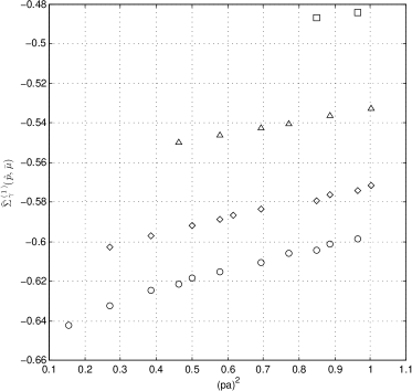
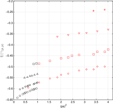
Figure 5: One-loop evaluation of $\widehat{\Sigma}_{\gamma}(\hat{p},\bar{\mu})$ (see Eq. (23)) on a $32^{4}$ lattice (left) and on both a $32^{4}$ and a $16^{4}$ lattice (right).

Why data arrange in families is clear from Eq. (23). On a finite lattice, the allowed (dimensionless) momenta are of the form

$$\hat{p}_{\mu}={{2\pi}\over{N}}n_{\mu},$$ (24)

where the $n_{\mu}$ are integer numbers. Given a 4-tuple $\{n_{1},n_{2},n_{3},n_{4}\}$, the values of the scalar functions $\hat{\Sigma}_{\gamma}^{(i)}(\hat{p})$ are fixed. Depending on the choice of the direction $\bar{\mu}$ in the right-hand side of Eq. (22), one gets different combinations of the $\hat{\Sigma}_{\gamma}^{(i)}(\hat{p})$ (depending on the length $|\hat{p}_{\bar{\mu}}|$) and thus different values for $\widehat{\Sigma}_{\gamma}(\hat{p},\bar{\mu})$. To be definite: suppose we pick the 4-tuple $\{1,1,1,2\}$. (this is the second lowest value of $\sum_{\nu}\hat{p}_{\nu}^{2}$ in Figure 5). When $\bar{\mu}=1,2,3$ we get the point on the first family (by this we mean the lowest lying, i.e. the circles), while for $\bar{\mu}=4$ we get the point on the second family (i.e. the diamonds). In other words, there is a different family for each different value of the length $|\hat{p}_{\mu}|$.

As a first attempt, we can fit Eq. (23) to our data by first (possibly) subtracting leading logs and then taking for each $\hat{\Sigma}_{\gamma}^{(i)}(\hat{p})|_{\mbox{\tiny{log subtr}}}$ an expansion in hypercubic invariants, e.g.

$$\hat{\Sigma}_{\gamma}^{(i)}(\hat{p})|_{\mbox{\tiny{log subtr}}}=c_{1}^{(i)}+c_{2}^{(i)}\sum_{\nu}\hat{p}_{\nu}^{2}+c_{3}^{(i)}{{\sum_{\nu}\hat{p}_{\nu}^{4}}\over{\sum_{\nu}\hat{p}_{\nu}^{2}}}+\mathcal{O}(a^{4}).$$ (25)

A trivial power-counting fixes the order at which each $\hat{\Sigma}_{\gamma}^{(i)}(\hat{p})$ is expanded (there is a factor of $\hat{p}^{2i}_{\bar{\mu}}$ in front). The only term surviving the $a\to 0$ limit is $c_{1}^{(0)}$, which is the only one we are interested in. Referring to the data of Figure 5, it is the estimate of $z_{q1}^{(0)}$, the finite part of the one-loop $Z_{q}$, as obtained from the computation on a $32^{4}$ lattice.

We do not report results for $Z_{q}$: in the following the dependence on $Z_{q}$ of Eq. (3) will be eliminated by making use of the quantity $\widehat{\Sigma}_{\gamma}(\hat{p},\bar{\mu})$ defined in Eq. (23), but before we can deal with this, we have to address the finite volume effects issue.

5.2 General procedure: disentangling finite volume effects

In Figure 5 (right) we display the computation of the one-loop $\widehat{\Sigma}_{\gamma}(\hat{p},\bar{\mu})$ on both a $32^{4}$ (black symbols) and a $16^{4}$ (red symbols) lattice. The 4-tuples $n_{\mu}$ defining the momenta are the same for measurements on both lattice sizes (as one can see, there is the same number of black and red symbols). Families join quite smoothly, in a way which is dictated by Eq. (24). Suppose we pick the same 4-tuple $\{1,1,1,2\}$ both on $32^{4}$ and on $16^{4}$ and inspect the values of $\widehat{\Sigma}_{\gamma}(\hat{p},\bar{\mu})$: we have to look for them (a) at different values of the abscissa $\sum_{\nu}\hat{p}_{\nu}^{2}$ and (b) on different families. To make the last point even clearer, consider the choice $\bar{\mu}=1$: on $32^{4}$ it results in $|\hat{p}_{\bar{\mu}}|=\pi/16$ and makes $\widehat{\Sigma}_{\gamma}(\hat{p},\bar{\mu}=1)$ fall on the first family (circles); $\bar{\mu}=1$ on $16^{4}$ results in $|\hat{p}_{\bar{\mu}}|=\pi/8$ and makes $\widehat{\Sigma}_{\gamma}(\hat{p},\bar{\mu}=1)$ fall on the second family (diamonds).

If there were no finite size effects, all the families should join in a perfectly smooth way and there should be a few points falling exactly on top of each other, e.g. the value of $\widehat{\Sigma}_{\gamma}(\hat{p},\bar{\mu})$ for the 4-tuple $\{1,1,1,1\}$ on $16^{4}$ should fall on top of the one associated to the 4-tuple $\{2,2,2,2\}$ on $32^{4}$. By inspecting the data ($\{1,1,1,1\}$ corresponds to the lowest value of $\sum_{\nu}\hat{p}_{\nu}^{2}$ for both lattice sizes) we see that the red diamond does not fall exactly on top of black one. This is a first hint at some finite size effect.

To correct for finite size effects we proceed along the lines that were first introduced in [4, 5]. We infer a $pL$ dependence in $\widehat{\Sigma}_{\gamma}$ (this is expected on dimensional grounds) and define a correction with respect to the infinite volume result by simply adding and subtracting the latter

$$\widehat{\Sigma}_{\gamma}(\hat{p},pL,\bar{\mu}) = \widehat{\Sigma}_{\gamma}(\hat{p},\infty,\bar{\mu})+\left(\widehat{\Sigma}_{\gamma}(\hat{p},pL,\bar{\mu})-\widehat{\Sigma}_{\gamma}(\hat{p},\infty,\bar{\mu})\right)$$ (26)

$$\equiv \widehat{\Sigma}_{\gamma}(\hat{p},\infty,\bar{\mu})+\Delta\widehat{\Sigma}_{\gamma}(\hat{p},pL,\bar{\mu})$$

To a first approximation we now let

$$\Delta\widehat{\Sigma}_{\gamma}(\hat{p},pL,\bar{\mu})\sim\Delta\widehat{\Sigma}_{\gamma}(pL),$$ (27)

the main rationale being that we neglect corrections on top of corrections (more on this later). As a result, we have a better form to be fitted to $\widehat{\Sigma}_{\gamma}|_{\mbox{\tiny{log subtr}}}$, e.g. (we here assume a low order expansions in terms of $a$, actually lower than the ones we typically manage)

$$\widehat{\Sigma}_{\gamma}(\hat{p},pL,\bar{\mu})|_{\mbox{\tiny{log subtr}}}=c_{1}^{(0)}+c_{2}^{(0)}\sum_{\nu}\hat{p}_{\nu}^{2}+c_{3}^{(0)}{{\sum_{\nu}\hat{p}_{\nu}^{4}}\over{\sum_{\nu}\hat{p}_{\nu}^{2}}}+c_{1}^{(1)}p^{2}_{\bar{\mu}}+\Delta\widehat{\Sigma}_{\gamma}(pL)+\mathcal{O}(a^{4}).$$ (28)

The above formula opens the way to a combined fit of measurements on different lattice sizes: since

$$p_{\mu}L={{2\pi n_{\mu}}\over{L}}L=2\pi n_{\mu},$$

there is only one finite size correction for each 4-tuple $n_{\mu}$ and no functional form has to be inferred for the correction.

The quantities $\widehat{\Sigma}_{\gamma}(\hat{p},pL,\bar{\mu})$ have been taken as examples to clarify the way we deal with the extraction of the continuum and infinite volume limits, but they are not directly used to determine the field renormalization $Z_{q}$. Without making explicit reference to $Z_{q}$ we instead rewrite the finite part of the currents RI’-MOM renormalization constants as

$$Z_{O_{\Gamma}}(\mu=p,\beta^{-1})|_{\mbox{\tiny{finite part}}}=\lim_{\begin{subarray}{c}a\rightarrow 0\\ L\rightarrow\infty\end{subarray}}{{\widehat{\Sigma}_{\gamma}(\hat{p},pL,\bar{\mu})}\over{\hat{O}_{\Gamma}(\hat{p},pL)}}|_{\mbox{\tiny{log subtr}}}$$ (29)

The right-hand side has to be evaluated order by order. The dependence on $Z_{q}$ has been traded for the $\widehat{\Sigma}_{\gamma}(\hat{p},pL,\bar{\mu})$, which reconstructs the $Z_{q}$ contribution to the left-hand side in the limits which are taken in Eq. (29). Before taking the limits this provides a lot of irrelevant contributions (and finite size effects) on top of what is per se contained in the $\hat{O}_{\Gamma}(\hat{p},pL)$, which are the finite lattice version of the $O_{\Gamma}(p)$ of Eq. (3). Here there is a subtlety connected with the dependence on direction of vector and axial currents: we will comment on this. Notice finally the notation $\ldots|_{\mbox{\tiny{log subtr}}}$: this means that the leading logarithms which plagues $Z_{O_{\Gamma}}(\mu=p,\beta^{-1})$ as a function of $pa$ have been subtracted (once again, they are known from the prescriptions of Section 2). The $a\rightarrow 0$ limit of Eq. (29) can be taken only provided this subtraction is performed.

Let’s consider the vertex function relevant for the computation of the vector current. In the continuum one has

$$\Gamma_{V}^{\mu}(p)=\gamma^{\mu}\,\Sigma_{V}^{(1)}(p^{2})+{{p^{\mu}\not{p}}\over{p^{2}}}\,\Sigma_{V}^{(2)}(p^{2})$$

where the extra contribution (with respect to the tree level structure) vanishes at $p=0$. The lattice version, due to the same mechanism which is place for $\hat{\Sigma}_{\gamma}$ (i.e. reduced symmetry with respect to the continuum), reads

$$\hat{\Gamma}_{V}^{\mu}(\hat{p})=\gamma^{\mu}\,\hat{\Sigma}_{V}^{(1)}(\hat{p})+{{\hat{p}^{\mu}\sum_{\nu}\gamma_{\nu}\hat{p}_{\nu}}\over{\sum_{\nu}\hat{p}_{\nu}^{2}}}\,\Sigma_{V}^{(2)}(\hat{p})+{{\hat{p}^{\mu 3}\sum_{\nu}\gamma_{\nu}\hat{p}_{\nu}}\over{\sum_{\nu}\hat{p}_{\nu}^{2}}}\,\Sigma_{V}^{(3)}(\hat{p})+{{\hat{p}^{\mu}\sum_{\nu}\gamma_{\nu}\hat{p}_{\nu}^{3}}\over{\sum_{\nu}\hat{p}_{\nu}^{2}}}\,\Sigma_{V}^{(4)}(\hat{p})+\ldots$$

where we have only written the first two irrelevant extra-contributions; the $\Sigma_{V}^{(i)}(\hat{p})$ depend on all the hypercubic invariants. If we now choose $\gamma_{\mu}$ as the projector $\hat{P}_{O_{\Gamma}}$ of Eq. (2) we would get a dependence on the direction (i.e. we would get a $\hat{O}_{\Gamma}(\hat{p},pL,\bar{\mu})$, in the notation which should by now be familiar). While this is not per se a conceptual problem, it is a practical one, since we would have a very large set of coefficients to fit. We can consider

$${{1}\over{12}}\left(\mbox{Tr}\;\gamma_{\mu}\hat{\Gamma}_{V}^{\mu}(\hat{p})-\mbox{Tr}\;{{\hat{p}^{\mu}\sum_{\nu}\gamma_{\nu}\hat{p}_{\nu}}\over{\sum_{\nu}\hat{p}_{\nu}^{2}}}\hat{\Gamma}_{V}^{\mu}(\hat{p})\right)\;\;\;\;\;\;\mbox{or}\;\;\;\;\;\;{{1}\over{4}}\sum_{\mu}\mbox{Tr}\;\gamma_{\mu}\hat{\Gamma}_{V}^{\mu}(\hat{p})$$

in order to have no dependence on direction. In the first case the contribution from $\Sigma_{V}^{(2)}(\hat{p})$ is eliminated at any value of the momentum, but we verified that the two procedures returns consistent results once irrelevant contributions are extrapolated away.
The procedure of averaging over directions would cancel the dependence on direction also in $\widehat{\Sigma}_{\gamma}(\hat{p},pL,\bar{\mu})$, but as we saw this dependence provides a very effective handle for assessing finite size effects. All in all, by retaining dependence on direction in $\widehat{\Sigma}_{\gamma}(\hat{p},pL,\bar{\mu})$ and eliminating a possible dependence on direction in $\hat{O}_{\Gamma}(\hat{p},pL)$ we aim at a fit which is both effective and not too demanding in terms of number of parameters.

From our NSPT computations we can evaluate (order by order) the quantities

$$\widehat{O}_{\Gamma}(\hat{p},pL,\bar{\mu})\equiv{{\widehat{\Sigma}_{\gamma}(\hat{p},pL,\bar{\mu})}\over{\hat{O}_{\Gamma}(\hat{p},pL)}}|_{\mbox{\tiny{log subtr}}}$$ (30)

where (compares to Eq. (29)) no limit is taken. The continuum and infinite volume limits are reconstructed by first computing the $\widehat{O}_{\Gamma}(\hat{p},pL,\bar{\mu})$ at different values of $(\hat{p},pL,\bar{\mu})$ and then fitting the results accordingly to the procedure we described above, for which we now provide a few extra details (see also [4, 5]). In practice we proceed as follows:

• A given $\widehat{O}_{\Gamma}(\hat{p},pL,\bar{\mu})$ is computed on different sizes $N=L/a$ and for different values of lattice momenta. We stress once again that the definition of $\widehat{O}_{\Gamma}(\hat{p},pL,\bar{\mu})$ entails the subtraction of leading logs contributions.

• We select a given interval of values of $\sum_{\nu}\hat{p}_{\nu}^{2}$: let’s call it $I_{p2}$. We also decide a given order for our fit in terms of power of $pa$. This fixes the number of parameters we have to determine as for irrelevant $pa$ contributions (we recall once again that this is fixed by hypercubic symmetry).

• Given the momentum interval and the sizes $N$, we define the set of points (i.e. 4-momenta) to be fitted by first selecting 4-tuples $\{n_{1},n_{2},n_{3},n_{4}\}$ satisfying the following requirement: the corresponding 4-momenta should return a value of $\sum_{\nu}\hat{p}_{\nu}^{2}$ within the selected momentum interval $I_{p2}$ for each value of $N$. Notice that within the approximation of Eq. (27) there is one parameter to be fitted for each of these 4-tuples: let’s call it $\Delta\widehat{O}_{\Gamma}(pL)$.

• We add to the set of momenta selected above the measurement taken on the largest lattice size $N_{\mbox{\tiny{max}}}$ at the 4-momentum corresponding to the largest value of $\sum_{\nu}\hat{p}_{\nu}^{2}$ within $I_{p2}$. This data point is assumed free of finite size effects and acts as a normalization point for our fitting procedure (we study the stability of the fit by allowing the inclusion of two data points from the largest lattice size, i.e. the two 4-momenta corresponding to the largest and second largest value of $\sum_{\nu}\hat{p}_{\nu}^{2}$ within $I_{p2}$).

• The functional form of our fit (and the number of parameters to be determined) is now completely fixed. In particular, no attempt is made to fit subleading logs.

One has to be aware that a number of assumptions were made, so that the effectiveness of the fit has always to be assessed a posteriori (at one-loop we can compare to results available from standard techniques; at higher loops we can assess stability of the procedure and inspect the values of standard indicators, e.g. values of $\chi^{2}$).

We plot in Figure 6 the one-loop $\widehat{O}_{S}(\hat{p},pL,\bar{\mu})$ (the $\widehat{O}_{\Gamma}(\hat{p},pL,\bar{\mu})$ for the scalar current). On the left, data are plotted as obtained on $32^{4}$ (black symbols) and $16^{4}$ (red symbols), without any finite size corrections. Finite size effects are manifest: red and black diamonds fail to fall on a smooth curve, and the same holds for black and red squares (these are supposed to be families in the jargon we introduced). On the right, we display the same data corrected for finite size effects: the corrections have been fitted according to our simplest recipe (in the spirit of Eq. (27)). Black and red diamonds and black and red squares now do fall on smooth curves. The effectiveness of the fit is displayed in Figure 7, where in particular one can see how well we determine the final result we are interested in, i.e. $z_{S1}^{(0)}$, in the notation of Eq. (16) (we recall that this is the counterpart of $c_{1}^{(0)}$ of Eq. (28)).

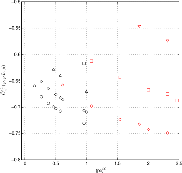
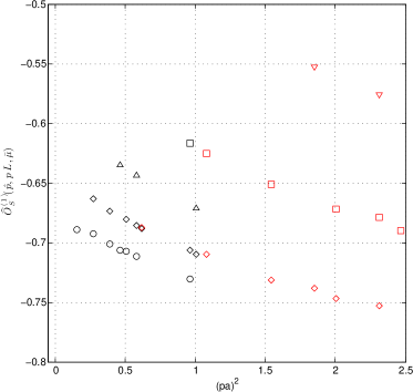
Figure 6: One-loop $\widehat{O}_{S}(\hat{p},pL,\bar{\mu})$ (see Eq. (30)) measured on a $32^{4}$ (black) and a $16^{4}$ (red) lattice, without (left) and with (right) finite size corrections.

Notice that finite size effects are more manifest in Figure 6 than in Figure 5. The latter refers to a quantity for which there is no log involved (the one-loop field anomalous dimension vanishes in Landau gauge). In [3] it was observed that whenever logs are in place, finite size effects can be quite large. This is a rationale in support of the strong assumption contained in Eq. (27), which states that we look for one single parameter ($\Delta\widehat{O}_{\Gamma}(pL)$) to correct for finite size effects in $\widehat{O}_{\Gamma}(\hat{p},pL,\bar{\mu})$. In the definition of the latter a subtraction of leading logs is in place. One can infer that on a finite lattice logarithmic divergences are actually regulated in the IR (see the discussion of [3] in terms of tamed logs). As a matter of fact, the finite size corrections that we get for finite renormalization constants (i.e. those of the vector and axial currents) are small, and results are within errors quite consistent with those obtained by taking into account only $32^{4}$ data.

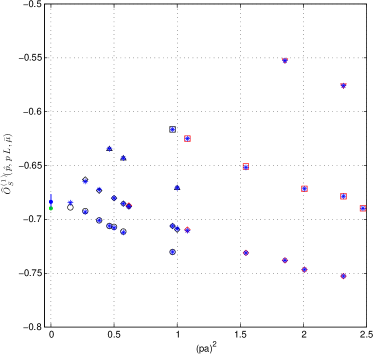
Figure 7: One-loop $\widehat{O}_{S}(\hat{p},pL,\bar{\mu})$ (see Eq. (30)) measured on a $32^{4}$ (black) and a $16^{4}$ (red) lattice, with finite size corrections and the fitted form plotted on top of data

6 Results: three-loop expansion of $Z_{S}$, $Z_{P}$, $Z_{V}$, $Z_{A}$

In Table 2 we report the coefficients of the three-loop expansion of $Z_{S}$, $Z_{P}$, $Z_{V}$ and $Z_{A}$. The expansion parameter is $\beta^{-1}$. We quote the analytical one-loop results [13]: the comparison confirms the effectiveness of our method. Errors are dominated by the stability of fits with respect to the change of fitting ranges, functional forms, number of lattice sizes simultaneously taken into account. Three-loop results for $Z_{S}$ and $Z_{P}$ have the indetermination in the coupling matching as an extra source of error (see discussion in Section 3).

Non-perturbative results for the quantities we computed are available in [8], where Twisted-Mass fermions regularization is in place for the same (RI’-MOM) renormalization scheme. The latter is defined in the chiral limit, and hence results must be the same as for Wilson fermions (our case). In order to make a comparison, we have to sum our series. The computations of [8] are at three values of $\beta$, namely $3.8$, $3.9$, $4.05$. The last one is in principle the best suited for a comparison in PT.

Table 2: One-, two- and three-loop coefficients of the renormalization constants for quark bilinears. Expansions are in $\beta^{-1}$. One-loop analytical results are reported for comparison.

	analytical
	one-loop	one-loop	two-loop	three-loop
$Z_{S}$	-0.6893	-0.683(7)	-0.777(24)	-1.96(14)
$Z_{P}$	-1.1010	-1.098(11)	-1.299(38)	-3.19(21)
$Z_{V}$	-0.8411	-0.838(6)	-0.891(17)	-1.870(65)
$Z_{A}$	-0.6352	-0.633(4)	-0.611(16)	-1.198(57)

The simplest (and straightforward) recipe is to sum the series in the coupling $\beta^{-1}$. At $\beta=4.05$ this results in $Z_{V}(\beta=4.05)=0.710(28)$, $Z_{A}(\beta=4.05)=0.788(18)$, $Z_{S}(\beta=4.05)=0.753(30)$, $Z_{P}(\beta=4.05)=0.610(48)$. Here we adhere to a standar recipe for pinning down an (order of magnitude for the) error: it is the three-loop contribution itself. At this stage one can inspect not too big discrepancies with the values reported in [8] for the finite renormalization constants (actually $Z_{A}$ is de facto fully consistent). Larger deviations are inspected for $Z_{S}$ and $Z_{P}$.

It has become very popular [21] to sum LPT results making use of different couplings, a procedure that is often generically referred to as Boosted Perturbation Theory (BPT). As our group also observed in [3], there is a large fraction of arbitrariness in one-loop BPT. Having three-loop results available provides a by far more stringent control. We will devote much more space to this in [6]. Here we merely quote that the use of different couplings (much the same was done in [3]) makes $Z_{V}$ and $Z_{A}$ fully consistent with the non-perturbative results of [8], while for $Z_{S}$ and $Z_{P}$ the agreement improves, but it is not full. We notice that these are the cases for which in our case it was crucial to look for finite size effects corrections.

7 Conclusions and prospects

The main message of this paper is that computing three-loop renormalization constants for Lattice QCD is fully viable, both for finite and for logarithmically divergent quantities. The control on both finite lattice spacing and finite volume effects appears solid and reliable.

While three-loop finite renormalization constants are fully consistent with non-perturbative results, the logarithmically divergent $Z_{S}$ and $Z_{P}$ are not. One should keep in mind that a typical RI’-MOM lattice computation is performed over a range of momenta eventually pinching the IR region. Now, contributions at low momenta are from one side supposed to be relevant in assessing irrelevant (UV) contributions (higher powers of $pa$ are suppressed), from another side prone to suffer from finite size (IR) effects. All in all, there is a subtle interplay of UV and IR effects.

We proposed a computational scheme to take control over this interplay in our perturbative framework. In [6], which is dedicated to three-loop computations in a different gluonic regularization (Iwasaki action), we devote more attention to quantify the impact of irrelevant and finite volume contributions, comparing results for the two different gluonic action (TLS and Iwasaki). It is important to keep in mind that the numerics of IR effects that we compute in LPT are not supposed to be the same of non-perturbative computations, while there is quite a consensus that this is the case for irrelevant (UV) ones. In [6] we discuss what of our approach could be relevant for the non-perturbative framework in terms of methodology.

References

- [1] F. Di Renzo, E. Onofri, G. Marchesini and P. Marenzoni, Four loop result in SU(3) lattice gauge theory by a stochastic method: Lattice correction to the condensate, Nucl. Phys. B 426, 675 (1994).
- [2] F. Di Renzo and L. Scorzato, Numerical Stochastic Perturbation Theory for full QCD, JHEP 04 (2004) 073.
- [3] F. Di Renzo, V. Miccio, L. Scorzato and C. Torrero, High-loop perturbative renormalization constants for Lattice QCD. I. Finite constants for Wilson quark currents, Eur. Phys. J. C 51, 645 (2007).
- [4] F. Di Renzo, E. -M. Ilgenfritz, H. Perlt, A. Schiller and C. Torrero, Two-point functions of quenched lattice QCD in Numerical Stochastic Perturbation Theory. (I) The ghost propagator in Landau gauge, Nucl. Phys. B 831, 262 (2010).
- [5] F. Di Renzo, E. -M. Ilgenfritz, H. Perlt, A. Schiller and C. Torrero, Two-point functions of quenched lattice QCD in Numerical Stochastic Perturbation Theory. (II) The Gluon propagator in Landau gauge, Nucl. Phys. B 842, 122 (2011).
- [6] M. Brambilla, F. Di Renzo and M. Hasegawa, High-loop perturbative renormalization constants for Lattice QCD (III): three-loop quark currents for Iwasaki gauge action and Wilson fermions, to be issued soon.
- [7] M. Hasegawa, M. Brambilla and F. Di Renzo, Three loops renormalization constants in Numerical Stochastic Perturbation Theory, PoS LATTICE 2012, 240 (2012).
- [8] M. Constantinou et al. [ETM Collaboration], Non-perturbative renormalization of quark bilinear operators with (tmQCD) Wilson fermions and the tree-level improved gauge action, JHEP 1008, 068 (2010).
- [9] B. Blossier et al. [ETM Collaboration], Renormalisation constants of quark bilinears in lattice QCD with four dynamical Wilson quarks, PoS LATTICE 2011, 233 (2011).
- [10] F. de Soto and C. Roiesnel, On the reduction of hypercubic lattice artifacts, JHEP 0709 (2007) 007.
- [11] G. Martinelli, C. Pittori, C. T. Sachrajda, M. Testa and A. Vladikas, A General method for nonperturbative renormalization of lattice operators, Nucl. Phys. B 445, 81 (1995).
- [12] J. A. Gracey, Three loop anomalous dimension of nonsinglet quark currents in the RI-prime scheme, Nucl. Phys. B 662, 247 (2003).
- [13] S. Aoki, K. i. Nagai, Y. Taniguchi and A. Ukawa, Perturbative renormalization factors of bilinear quark operators for improved gluon and quark actions in lattice QCD, Phys. Rev. D 58, 074505 (1998).
- [14] A. Skouroupathis and H. Panagopoulos, Two-loop renormalization of scalar and pseudoscalar fermion bilinears on the lattice, Phys. Rev. D 76, 094514 (2007) [Erratum-ibid. D 78, 119901 (2008)]
- [15] F. Di Renzo, L. Scorzato, The Residual mass in lattice heavy quark effective theory to order, JHEP 0102 (2001) 020.
- [16] F. Di Renzo, L. Scorzato, The residual mass in perturbative lattice-HQET for an improved determination of , JHEP 0411 (2004) 036.
- [17] Y. Schroder, The Static potential in QCD to two loops, Phys. Lett. B 447 (1999) 321.
- [18] M. Brambilla and F. Di Renzo, Matching the lattice coupling to the continuum for the tree level Symanzik improved gauge action,’ PoS LATTICE 2010 (2010) 222.
- [19] A. Skouroupathis, M. Constantinou, H. Panagopoulos, Two-loop additive mass renormalization with clover fermions and Symanzik improved gluons, Phys. Rev. D77 (2008) 014513.
- [20] D. Hesse, M. Dalla Brida, S. Sint, F. Di Renzo, M. Brambilla The Schrödinger Functional in Numerical Stochastic Perturbation Theory, PoS LATTICE 2013 (2013) 325.
- [21] G. P. Lepage and P. Mackenzie, On the viability of lattice perturbation theory, Phys. Rev. D48 (1993) 2250.