A temporal steering inequality

Abstract

Quantum steering is the ability to remotely prepare different quantum states by using entangled pairs as a resource. Very recently, the concept of steering has been quantified with the use of inequalities, leading to substantial applications in quantum information and communication science. Here, we highlight that there exists a natural temporal analogue of the steering inequality when considering measurements on a single object at different times. We give non-trivial operational meaning to violations of this temporal inequality by showing that it is connected to the security bound in the BB84 protocol and thus may have applications in quantum communication.

I Introduction

Non-locality is one of the most striking concepts of quantum mechanics in that it defies our intuition about space and time. Its history can be traced back to such early works as those of Einstein, Podolsky, and Rosen EPR . After Bell proposed his famous test of non-locality in 1964 Bell , almost all experimental implementations have yielded violations of his inequalities Aspect . Motivated by the advance of quantum information science, quantum non-locality as a resource has been further studied in the form of entanglement and entanglement measures. Recently, an inequality to delineate quantum steering from other non-local properties was proposed Wiseman ; Caval ; Smith and tested in a range of experiments Smith ; experiments . Steerability has since then been further investigated with all-versus-nothing measures JingLing , and has been utilized as a way to characterize and visualize the state-space of two-qubit systems Jevtic . In combination these different concepts (Bell non-locality, steerability, and entanglement) form a hierarchy and enable one to categorize different non-local properties of quantum states.

Moving away from the notion of non-locality, Leggett and Garg in 1985 derived an inequality LG to test the assumption of “macroscopic realism” on a single object. An experimental violation of this inequality has been observed in a large range of systems over the last few years SC ; EmaryReview . In addition, the Leggett-Garg (LG) inequality can also be applied to microscopic systems Lambert1 ; Lambert2 ; SR1 ; SR2 , as a tool to examine the quantum coherent dynamics therein. For two-level systems, there is a one-to-one correspondence between the LG inequality and the Bell-CHSH inequality Brukner , a fundamental consequence of the Choi-Jamiolkowski isomorphismchoi .

Since the steering inequality is fundamentally linked to the notion of non-locality we then ask the following question: Does there exist a temporal scenario or analogue of the steering inequality, as implied by the Choi-Jamiolkowski isomorphism, and does it have any non-trivial implications? We start by showing, in Section II, that there does exist such an analogue, and in Section III give some simple examples of its behavior. To give a non-trivial operational meaning to this temporal steering inequality in Section IV we show that, for a noisy channel, the upper bound on the noise which limits the observation of a violation of temporal steering exactly corresponds to the optimal upper limit on the allowable noise in the BB84 quantum cryptography scheme BB84 . In Section V we discuss how spatial and temporal steering can be distinguished.

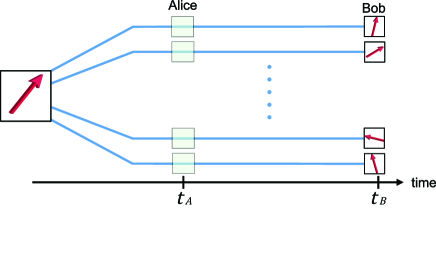
Figure 1: (Color online) Temporal scenario of the steering inequality. An object may be sent into different channels with probability distribution $q_{\lambda}$. Alice claims that the non-invasive measurement is performed at the earlier time $t_{A}$, whereas Bob performs the trusted quantum measurement at the later time $t_{B}$.

II Formulation

First, consider a quantum channel through which a system is sent to Bob. At an intermediate point of the channel, Alice can perform some operations, including measurements on the system, before Bob receives the system and performs his measurement. The state of the system is characterized by a set of observables. In this setting, Alice measures the observable $A_{i}$ at time $t_{\mathrm{A}}$, and subsequently Bob measures the observable $B_{j}$ at $t_{\mathrm{B}}$. The subscripts $i$ and $j$ are the particular choice of observable each makes. For example, for a two-level system, when Bob performs his measurements with a mutually-unbiased basis (e.g., Ref. [Wootters;Fields:1989, ]), the corresponding observables are $B_{1}=\sigma_{z}$, $B_{2}=\sigma_{x}$, and $B_{3}=\sigma_{y}$. When the measurement results of $A_{i}$ and $B_{j}$ are, respectively, $a$ and $b$, the joint probability distribution of this result is

$$P^{\mathrm{Q}}(A_{i,t_{\mathrm{A}}}=a,\,B_{j,t_{\mathrm{B}}}=b)$$

$$\quad\quad=P^{\mathrm{Q}}(A_{i,t_{\mathrm{A}}}=a)P^{\mathrm{Q}}(B_{j,t_{\mathrm{B}}}=b|A_{i,t_{\mathrm{A}}}=a).$$ (1)

We explicitly write the measurement times as subscripts of the observables. The conditional probability $P^{\mathrm{Q}}(B_{j,t_{\mathrm{B}}}=b|A_{i,t_{\mathrm{A}}}=a)$ is an expectation value of a projector (or a positive operator related to a positive operator-valued measure) with respect to a density matrix depending on a Alice’s measurement result. In other words, this quantity contains the backaction from Alice’s measurement. This backaction can change the quantum dynamics after the measurement.

Now, to obtain a temporal steering-inequality, we consider an alternative model to describe the aforementioned scenario. In this model, Bob receives a system that is sent to him through one of several different channels, chosen randomly, as seen in Fig. 1. Furthermore, the choice of Alice’s measurement observable has no influence on the state of the system Bob receives, apart from furnishing information about which channel it is sent through. In the temporal scenario this can only arise from variations of three possible scenarios; first, Alice simply does not have access to Bob’s system, and is “making-up” her measurement results. Second, Alice does have access to Bob’s system but the influence of her measurement choice is washed out by the noise in the channel, before Bob receives the system. Third, Alice cannot measure Bob’s qubit, but can determine something about which channel the system passed through.

The above setting can be regarded as a multi-channel protocol with probability distribution $q_{\lambda}$, as seen in Fig. 1. The classical random variable $\lambda$ specifies a given type of channel. Both Alice and Bob do not have a priori knowledge about $q_{\lambda}$. We assume that: (i) Bob trusts only his measurement results, and (ii) Alice’s choice of measurement has no influence on the state Bob receives. Instead of Eq. (1), the joint probability distribution can be written as

$$P(A_{i,t_{A}} = a,B_{j,t_{B}}=b)$$ (2)

$$= \sum_{\lambda}q_{\lambda}P_{\lambda}(A_{i,t_{\mathrm{A}}}=a)P_{\rho_{\lambda}}^{\mathrm{Q}}(B_{j,t_{\mathrm{B}}}=b)\text{,}$$

where $\sum_{\lambda}q_{\lambda}=1$. The conditional probability $P_{\lambda}(A_{i,t_{\rm A}}=a)$ is associated with Alice’s (non-invasive) measurement at time $t_{\mathrm{A}}$. The quantum state for the channel $\lambda$ is evolved into $\rho_{\lambda}$ at time $t_{\mathrm{B}}$. Bob obtains the conditional probability $P^{\rm Q}_{\rho_{\lambda}}(B_{j,t_{\rm B}}=b)$ as quantum mechanics gives (i.e., an expectation value with respect to $\rho_{\lambda}$).

Using Eq. (2) we can derive the temporal analogue of the steering inequality. Hereafter, we focus on the case when the object is a two-level (or a two-valued) system in which the observable takes either $+1$ or $-1$. The observables $A$ and $B$ are the Pauli matrices. We stress that the formula (2) is essentially the same as in the context of the (spatial) quantum steering inequality Wiseman , where the notion of non-invasive measurement is the analogue to locality. Following the techniques in Ref. Smith, , the temporal steering inequality is

$$S_{N}\equiv\sum_{i=1}^{N}E\left[\left\langle B_{i,t_{\mathrm{B}}}\right\rangle_{A_{i,t_{\mathrm{A}}}}^{2}\right]\leq 1,$$ (3)

where $N$($=2$ or $3$) is the number of mutually-unbiased measurements that Bob implements on his qubit, and

$$E\left[\left\langle B_{i,t_{\mathrm{B}}}\right\rangle_{A_{i,t_{\mathrm{A}}}}^{2}\right]\equiv\sum_{a=\pm 1}P(A_{i}=a)\left\langle B_{i,t_{\mathrm{B}}}\right\rangle_{A_{i,t_{\mathrm{A}}}=a}^{2},$$ (4)

with

$$P(A_{i,t_{\mathrm{A}}}=a)\equiv\sum_{\lambda}q_{\lambda}P_{\lambda}(A_{i,t_{\mathrm{A}}}=a),$$ (5)

and Bob’s expectation value conditioned on Alice’s result is defined as

$$\left\langle B_{i,t_{\mathrm{B}}}\right\rangle_{A_{i,t_{\mathrm{A}}}=a}\equiv\sum_{b=\pm 1}b\,P(B_{i,t_{\mathrm{B}}}=b\mid A_{i,t_{\mathrm{A}}}=a).$$ (6)

The inequality (3) comes from the fact two observables in a mutually-unbiased basis are non-commutative. If the inequality is violated, it implies Alice’s choice of measurement basis influences Bob’s measurement outcomes, and that the channel has not erased the influence of this choice.

III Examples

For illustrative purposes, we first consider an example of a single qubit that undergoes Rabi-oscillations due to the dynamics given by the Hamiltonian evolution $H^{\prime}=\hbar g(\sigma_{+}+\sigma_{-})$, where $g$ is the Rabi frequency, and $\sigma_{+}$ and $\sigma_{-}$ are the raising and lowering operators of the qubit. In addition, the qubit is also subject to an intrinsic Markovian decay process in Lindblad form, so that the total evolution of the density matrix can be expressed as

$$\dot{\rho}=\frac{1}{i\hbar}[H^{\prime},\rho]+\frac{\gamma}{2}(2\sigma_{-}\rho\sigma_{+}-\sigma_{+}\sigma_{-}\rho-\rho\sigma_{+}\sigma_{-}),$$ (7)

where $\gamma$ is the decay rate of the qubit. Assuming that the qubit is initially in the mixed state,

$$\rho_{t=0}=\left(\begin{array}[]{cc}\frac{1}{2}&0\\ 0&\frac{1}{2}\end{array}\right),$$ (8)

one first performs a measurement along the $\widehat{x}$, $\widehat{y}$, or $\widehat{z}$ direction at time $t_{A}=0$, to mimic the action of Alice in Fig. 1. After the system evolves to time $t$, the second measurement is implemented along a mutually unbiased basis. The various measurement outcomes are sorted and arranged conditionally, and the steering parameter is calculated.

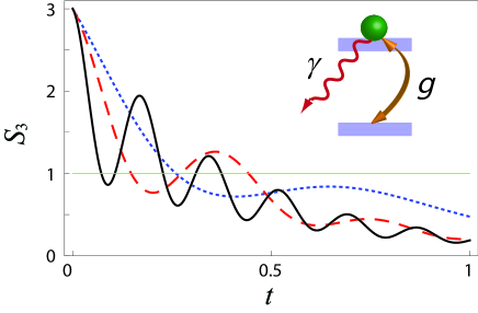
Figure 2: (Color online) The temporal steering parameter $S_{3}$ of a qubit initially prepared in the mixed state undergoes Rabi-oscillations with the coherent Rabi frequency $g$ and the intrinsic decay rate $\gamma$. In all figures $\hbar=1$. The black-solid, red-dashed, and blue-dotted curves represent the results of $g=9\gamma,$ $4\gamma$, and 2$\gamma$, respectively.

In Fig. 2, we plot the steering parameter $S_{3}$ as a function of the evolution time. For short times ($t\rightarrow 0$), the steering parameter always violates the bound and reaches the value of $3$. To understand this, let us recall the spatial steering inequality. Suppose Alice and Bob share a Werner state of visibility $V$,

$$\rho_{w}=V\left|\psi_{-}\right\rangle\left\langle\psi_{-}\right|+(1-V)/4,$$ (9)

where $\left|\psi_{-}\right\rangle\left\langle\psi_{-}\right|$ is the Bell singlet state. After Alice performs her measurements (along the $\widehat{x}$, $\widehat{y}$, and $\widehat{z}$ directions), some of the possible reduced, measurement-conditioned density matrices of Bob’s system before Bob’s measurements are made can be written as follows:

$$\rho_{\sigma_{z},+1} = \left(\begin{array}[]{cc}\frac{1-V}{2}&0\\ 0&\frac{1+V}{2}\end{array}\right),\rho_{\sigma_{x},+1}=\left(\begin{array}[]{cc}\frac{1}{2}&-\frac{V}{2}\\ -\frac{V}{2}&\frac{1}{2}\end{array}\right).$$ (14)

Since the steering parameter is the summation of the results along different unbiased bases, it is the differences in the coherence terms ($V$ in the off-diagonal element) that give the violation of the inequality.

Returning to the temporal analogue of the steering inequality, similar results occur. When Alice performs the first measurements along a certain basis, the qubit is projected into the corresponding state. From the viewpoint of a given basis (for example, the $\widehat{z}$ basis), the measurement creates coherence in the density matrix if the measurement is along another mutually unbiased $\widehat{x}$ or $\widehat{y}$ direction. If Bob immediately performs the second measurements after Alice’s measurement, the influence of Alice’s choice of measurement is as large as it can be, resulting in the violations of the bound. Another phenomenon worth mentioning is that the violation may re-occur at later times if the frequency $g$ is strong enough (compared with the decay rate $\gamma$). This feature resembles a similar effect in the Leggett-Garg inequality, where violations are periodic in time. In Appendix A, we consider an extension of this example, where revivals also occur due to strong interactions with a quantum environment. Ultimately, a violation of the temporal steering inequality means that there are significant quantum correlations between measurements at different times. However, unlike in the Leggett-Garg and Bell inequality cases one should be wary of implementing any version of the steering inequality as a kind of quantum witness, as it is of course trivially violated by a two-partite classical hidden variable model. A summary of the various spatial and temporal inequalities are given in Table 1.

CHSH Inequality	Leggett-Garg Inequality
$|\langle B_{1}A_{1}\rangle+\langle B_{1}A_{2}\rangle+\langle B_{2}A_{1}\rangle-\langle B_{2}A_{2}\rangle|\leq 2$	$|\langle A_{i,t_{2}}A_{i,t_{1}}\rangle+\langle A_{i,t_{3}}A_{i,t_{2}}\rangle+\langle A_{i,t_{4}}A_{i,t_{3}}\rangle-\langle A_{i,t_{4}}A_{i,t_{1}}\rangle|\leq 2$
Steering inequality	Temporal steering inequality
$\sum_{i=1}^{N}E\left[\left\langle B_{i}\right\rangle_{A_{i}}^{2}\right]\leq 1$	$\sum_{i=1}^{N}E\left[\left\langle B_{i,t_{\mathrm{B}}}\right\rangle_{A_{i,t_{\mathrm{A}}}}^{2}\right]\leq 1$

Table 1: A summary of the definitions of the various spatial and temporal inequalities. Particular examples of the spatial inequalities (the Bell inequality and the steering inequality) are shown on the left, with their corresponding temporal analogues on the right.

IV Quantum Cryptography

It is well known that the spatial steering inequality has some promising applications in quantum communication and quantum cryptography app ; Smith . Here, we discuss how the temporal steering inequality has directly analogous applications. In particular, as with the spatial steering inequality app and the CHSH inequalitycryptography , the temporal steering inequality can be used to directly test the suitability of a quantum channel for certain quantum cryptography protocols. However, unlike the spatial steering inequality, one does not need to resort to entanglement based schemes but can directly work with the BB84 and related protocols BB84 ; app ; 1sided .

Typically, in the BB84 protocol one needs to check whether a state sent from Alice to Bob, from which they wish to construct their private key, is being measured by a third person, Eve. To do this, Alice and Bob have to compare their measurement results using a sub-ensemble of their qubits. The eavesdropping by Eve is equivalent to an environment acting on the quantum state, or losses in a noisy channel. Thus in any real implementation of BB84 there is an upper-limit to how noisy the channel can be; otherwise the possible effect of Eve’s measurements cannot be distinguished from that noise.

As an example, let us evaluate the average bit error rate that Alice and Bob will find when the channel is influenced by Eve’s measurements. Alice performs her projective measurement on an initial state $\rho_{0}$, producing the state $\rho_{\mathrm{A},\mu}$, with $\mu=(i,a)$. The subscript $\mu$ represents the choice of measurement direction ($i=\widehat{z},\,\widehat{x}$) and the measured value ($a=\pm 1$). Alice then sends this state to Bob through a quantum channel, during which Eve tries to eavesdrop and measure the state of the system. We denote the state Bob receives as $\rho_{\mathrm{B},\mu}$. The average bit error rate can be written by

$$R_{\mathrm{err}}=\frac{1}{2}\sum_{\mu}P^{\mathrm{Q}}(A_{i,t_{\mathrm{A}}}=a)\left[1-\mathrm{Tr}(\sqrt{\rho_{\mathrm{A},\mu}}\rho_{\mathrm{B},\mu}\sqrt{\rho_{\mathrm{A},\mu}})\right].$$ (15)

During the eavesdropping, Eve randomly measures the qubit along the $\widehat{z}$ ($\widehat{x}$) direction with probability $q$ ($p$) or does nothing with probability $1-(p+q)$ (under the constraint of $p+q\leq 1$). The effect of this process on the state that Bob receives can be shown to be (see Appendix C),

$$R_{\mathrm{err}}=\frac{1}{4}(p+q).$$ (16)

What is the minimum error that Eve can introduce and still gain sufficient information to capture the shared key of Alice and Bob? The optimal upper bound cryptography allowable in a quantum channel so that the channel is still useful for BB84, and in corollary the minimum error rate Eve can induce while still extracting useful information, is in the case when the effect of Eve’s actions in each basis is equal, i.e., when $p=q$. When Eve adopts a strategy that relies just on independent attacks on each qubit the optimal scenario was found cryptography ; cryptographyOLD to be set by the equation $2(1-2R_{\mathrm{err}})^{2}-1=0$, which gives a threshold error rate of $R_{\mathrm{err}}(p=q)=0.146447$.

How are BB84 and the error rate of a channel related to temporal steering? Since Eve’s action can be described as a quantum channel (see appendix B) we can see a direct relationship between the error rate and the violation of the temporal steering inequality; if the loss in the channel is too large the steering inequality is not violated. To make things concrete we focus on the temporal steering parameter for $N=2$, This is a reasonable choice, because in the standard BB84 scheme one performs measurements along either $\widehat{z}$ or $\widehat{x}$ directions. One finds that, for the quantum channel described above,

$$S_{2}=(1-p)^{2}+(1-q)^{2}.$$ (17)

As shown in Fig. 3, Eq. (3) implies an upper bound of $S_{2}$ equal to unity.

Considering the scenario mentioned above, when Eve’s measurements are equally distributed ($p=q$), from the roots of setting Eq. [17] equal to unity, one also finds that the steering inequality reduces to $2(1-2R_{\mathrm{err}})^{2}-1=0$: The steering inequality bound and the BB84 threshold are equivalent. In other words, the boundary of steerability is set by the optimal error rate for the BB84 protocol, and vice versa. A similar result was also observed by extending BB84 into an entanglement utilizing protocol, and calculating the violation of a Bell inequalityEkert .

However, $R_{\mathrm{err}}(p=q)=0.146447$ is still not the minimum noise that Eve can induce. She can resort to so-called “coherent” attacks where she can access multiple qubits and operate on them at the same time. In this case cryptography it was found that the minimum error rate was $11\%$. Recently Branciard et al. app showed that the key length in that case could be mapped to a different type of spatial steering inequality based on conditional entropies between Alice and Bob’s qubits, in analogy to the entropic Bell and Leggett-Garg inequalities entropicBell ; entropicLI ; entropic . One can again map this entropic steering inequality into the temporal domain, which has the same error bound as the spatial one, producing a temporal entropic steering inequality:

$$S_{2}^{(E)}\equiv\sum_{i=1}^{2}H(B_{i,t_{B}}|A_{i,t_{A}})\geq 1,$$

where the average conditional entropies are defined

$$H(B_{i,t_{B}}|A_{i,t_{A}})=\sum_{a=\pm 1}P(A_{i}=a)H(B_{i}|a),$$ (18)

and

$$H(B_{i}|a)=-\sum_{b=\pm}P(B_{i}=b|a)\mathrm{log}_{2}P(B_{i}=b|a).$$ (19)

One can again app relate this to a bit error rate (assuming it is again equal in both bases), which reduces to

$$1-2h(R_{\mathrm{err}})\leq 0,$$ (20)

where

$$h(R_{\mathrm{err}})=-R_{\mathrm{err}}\mathrm{log}_{2}R_{\mathrm{err}}-(1-R_{\mathrm{err}})\mathrm{log}_{2}(1-R_{\mathrm{err}}).$$ (21)

Ultimately, one may consider temporal steering inequalities as a benchmark for validating the usability of a quantum channel for BB84. The connection discussed here, between BB84 and steerability, is both natural and physical, because of the Choi-Jamiolkowski isomorphism choi and the known symmetry between BB84 and entanglement based protocols Ekert . However it allows one to consider BB84 protocols app ; 1sided in a practical and direct way. Possible generalization to other protocols Bruss deserves further investigation.

Finally, one may ask what are the relative merits of steerability versus full Bell non-locality in terms of their ability to characterize a quantum channel. For cryptography schemes based on entangled pairs, encoding using two mutually unbiased bases, and an eavesdropper strategy based on an independent attack, both the Bell inequality violation, the steering inequality violation, and BB84 are limited by the same bit error rate ($14.6\%$). In the entangled-based spatial scenario Alice and Bob typically attempt to share an entangled singlet state. The effect of Eve inducing errors on this state, due to measuring equally in two-bases, means that the state that Alice and Bob receive is a Werner state. The Werner state is one of the few states where the CHSH and steering inequality violations coincide. The result by Branciard et al. app discussed above suggests that in other situations steering inequalities, and thus steering as a resource, may be more useful for validating quantum channels than Bell non-locality (which is necessarily stricter).

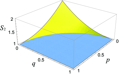
Figure 3: (Color online) The steering parameter $S_{2}$ under the disturbance by the third party, Eve, with the probabilities of measurements $q$ (along the $\widehat{z}$ direction) and $p$ (along the $\widehat{x}$ direction).

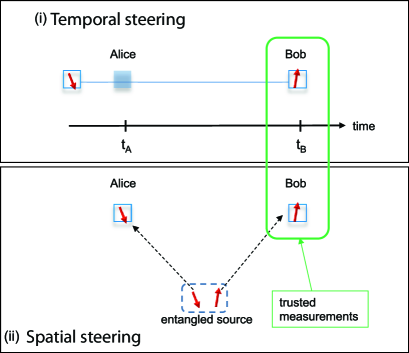
Figure 4: (Color online) Two possible situations that can lead to the violation of the steering inequality: (i) Bob’s particle is measured by Alice at a earlier time; (ii) Bob’s particle is entangled with another one, on which Alice performs measurement.

V Temporal Ordering

In a real scenario there is a further symmetry between the temporal and spatial steering inequalities. In both cases Bob trusts only his measurement results and asks Alice to provide her measurement outcomes to him for comparison. From Bob’s point of view, a violation of the inequality may have two possible origins (excluding non-local communication between his and Alice’s apparatus) (i) Bob’s particle is measured by Alice at a earlier time (temporal steering), or (ii) Bob’s particle is entangled with another one, on which Alice performs measurements (spatial steering).

To distinguish these two cases, the following steps could be made. (a) When Bob receives the particle, he should not perform his measurement immediately and also ask Alice not to perform her measurement (though of course she may already have done so, and on Bob’s qubit in the temporal scenario). (b) Bob should ask Alice to perform her measurement following his orders, e.g., along the $\widehat{x}$, $\widehat{y}$, or $\widehat{z}$ direction. (c) After Alice reports her measurement results, Bob then performs the corresponding measurement. If Alice has already pre-measured Bob’s qubit then, unless Bob chooses the basis she happens to have already pre-measured in, she can only make a random guess. On the other hand, for the case (ii), Alice can still measure her qubit and Bob’s results can be steered to give violations.

VI Conclusion

In summary, we have shown that there exists a temporal scenario of the steering inequality for a single object. A strong connection to the bound on the error rate of a quantum channel in the BB84 protocol is pointed out and may have potential applications in quantum communication Smith .

Appendix A Non-Markovian environment

When a system is coupled to an environment it is possible that coherence between the system and the environment, i.e., entanglement, can be created during the evolution. It is interesting to know if such a coherence can also cause recurrent violations of the temporal steering inequality. To investigate this we consider a single qubit coherently coupled to another ancillary qubit, which serves as an effective environment, as shown in the inset of Fig. 5. If one traces out the effective-environment-qubit the reduced system can be viewed as being coupled to a non-Markovian environment.

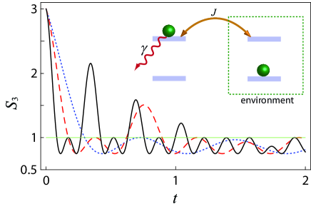
Figure 5: (Color online) The temporal steering parameter $S_{3}$ as a function of time. The black-solid, red-dashed, and blue-dotted curves represent the results of $J=9\gamma,$ $4\gamma$, and 2$\gamma$, respectively. Inset: Schematic view of a qubit coupled to a special environment (another qubit) with the coherent coupling strength $\hbar J$ and the intrinsic decay rate $\gamma$.

In addition to this effective environment, we assume that the system is subject to an intrinsic decay as in the example in the main text, but without the influence of the Rabi-oscillation-inducing Hamiltonian. The interaction between the system and the environment is written as $H_{\text{int}}=\hbar J(\sigma_{+}^{1}\sigma_{-}^{2}+\sigma_{+}^{2}\sigma_{-}^{1})$, where $\sigma_{+}^{i}$ and $\sigma_{-}^{i}$ are the raising and lowering operators of the $i$-th qubit, and $\hbar J$ is the coherent coupling between the system and the environment. The master equation of the total system is

$$\dot{\rho}=\frac{1}{i\hbar}[H_{\text{int}},\rho]+\frac{\gamma_{1}}{2}(2\sigma_{-}^{1}\rho\sigma_{+}^{1}-\sigma_{+}^{1}\sigma_{-}^{1}\rho-\rho\sigma_{+}^{1}\sigma_{-}^{1}),$$ (22)

where $\gamma_{1\text{ }}$is the decay rate of the system qubit. In Fig. 5, we plot the steering parameter $S_{3}$ for various coupling strengths $\hbar J$. Similar to the previous example, Fig. 2 in the main text, there are violations in the short-time regime. If the coupling $\hbar J$ is strong enough, it can also induce recurrent violations at later times. Again, the coherent coupling $\hbar J$ causes the recurrence of coherence in the system qubit. These coherent off-diagonal terms then give the violations of the inequality.

Appendix B Characterizing the dephasing of a quantum channel

It is interesting to know if there are other practical applications of the temporal steering inequality. To gain further insight, we analyze the various contributions the steering parameter $S_{3}$ for the example system discussed earlier, of a single qubit undergoing Rabi oscillations and decay processes (Fig. 2 in the main text). Interestingly, we find the contribution from the measurement in the $\widehat{x}$ direction is independent of the coherent Rabi frequency $g$ and takes the simple form

$$E\left[\left\langle\widehat{B}_{i}\right\rangle_{A_{i=\widehat{x}}}^{2}\right]=\exp(-2\gamma t),$$ (23)

while the contributions from the measurements in the $\widehat{z}$ and $\widehat{y}$ directions,

$$E\left[\left\langle\widehat{B}_{i}\right\rangle_{A_{i=\widehat{y}}}^{2}\right]~{}~{}\text{and}~{}~{}E\left[\left\langle\widehat{B}_{i}\right\rangle_{A_{i=\widehat{z}}}^{2}\right],$$ (24)

are functions of both $g$ and $\gamma$.

This means that the measurements in the $\widehat{x}$ direction are independent of the coherent tunneling amplitude $g$, and allow us to extract information about the dephasing rate $\gamma$ of the channel if we know in advance the axis of the coherent tunneling.

Generally speaking, $E\left[\left\langle\widehat{B}_{i}\right\rangle_{A_{i=\widehat{x}}}^{2}\right]$, $E\left[\left\langle\widehat{B}_{i}\right\rangle_{A_{i=\widehat{y}}}^{2}\right]$, and $E\left[\left\langle\widehat{B}_{i}\right\rangle_{A_{i=\widehat{z}}}^{2}\right]$ are influenced by both coherent and incoherent properties of the channel. Therefore, the value of the steering parameter can be used as an approximate indicator of how good a channel is. For example, if the value of the steering parameter $S_{2}$ is very close to $2$ after the qubit passes through the channel, one can expect it does not lose much of its coherence, and hence dephasing and losses are low. One can in principle check $S_{2}$ with and verify the quality of the channel, rather than doing full process tomographyNielsen . How this scales to larger dimensional systems is an interesting open problem.

Appendix C Method for assessing steering and error rates in the BB84 protocol

We now show a method for calculating the average error rate $R_{\mathrm{err}}$ and the temporal steering parameter $S_{2}$ in the BB84 protocol. Throughout this supplementary material, the temporal behavior of all quantities will be calculated in the Schrödinger picture.

Let us describe the BB84 protocol in terms of a quantum channel. A quantum object is initially prepared as a density matrix $\rho_{0}$. Subsequently, Alice performs her projective measurement on $\rho_{0}$, interacting a probe (ancillary) qubit with the object and measuring the probe system destructively. As a result, the object becomes a pure state $\rho_{\mathrm{A},i,a}=\Pi_{i,a}$, with probability $P^{\rm Q}(A_{i,t_{\rm A}}=a)={\rm Tr}\,(\Pi_{i,a}\rho_{0})$. The operator $\Pi_{i,a}$ is the projector onto the eigenvector of the $i$th component of the $2\times 2$ Pauli matrix ($i=\widehat{z},\widehat{x}$). When $i=\widehat{z}$, for example, we find that $\Pi_{\widehat{z},a}=|\widehat{z},a\rangle\langle\widehat{z},a|$, with $\sigma_{z}|\widehat{z},a\rangle=a|\widehat{z},a\rangle$ and $a=\pm 1$. Between Alice and Bob, Eve tries to eavesdrop the information sent. Eve’s action can be described by a linear map. For an input state $\rho$, one may write this linear map as the Kraus representation Nielsen ,

$$\rho\ \mapsto\ \mathcal{E}(\rho)=(1-p-q)\rho+q\,\pi_{\widehat{z}}(\rho)+p\,\pi_{\widehat{x}}(\rho),$$ (25)

with

$$\pi_{i}(\rho)=\sum_{a}\Pi_{i,a}\,\rho\,\Pi_{i,a},\;0\;\leq\;p\;,\;q\;\leq 1,$$ (26)

and $p+q\leq 1$. Therefore, Bob receives the density matrix $\rho_{{\rm B},i,a}=\mathcal{E}(\rho_{{\rm A},i,a})$. The process is assessed by the fidelity

$$F(\rho_{\mathrm{A},i,a},\,\mathcal{E}) = \mathrm{Tr}\,(\sqrt{\rho_{\mathrm{A},i,a}}\;\rho_{\mathrm{B},\mu}\,\sqrt{\rho_{\mathrm{A},i,a}})$$ (27)

$$= (1-p-q)\;+q\;\langle i,a\,|\pi_{z}(\rho_{\mathrm{A},i,a})|\,i,a\rangle$$

$$+p\,\langle i,a\,|\pi_{x}(\rho_{\mathrm{A},i,a})|\,i,a\rangle.$$

When this quantity is unity, the protocol completely works for a specific input state $\rho_{\mathrm{A},i,a}$. The error rate $R_{\mathrm{err}}$ is the mean value of $(1-F)$ over all possible input states.

The fidelity (27) is calculated as follows. First, we focus on the formula

$$|\langle\,i,a|\,j,b\rangle|=\delta_{i,j}\delta_{a,b}+\frac{1}{\sqrt{2}}(1-\delta_{i,j}).$$ (28)

The second term comes from the fact that $|\widehat{z},a\rangle$ and $|\widehat{x},a\rangle$ are the elements of the mutually-unbiased basis in a two-level system Wootters;Fields:1989 . Using this formula, we obtain

$$\langle i,b\,|\pi_{j}(\rho_{i,a})|\,i,b\rangle=\delta_{i,j}\mathrm{Tr}\,(\Pi_{j,b}\,\rho_{i,a})+\frac{1}{2}(1-\delta_{i,j}).$$ (29)

Furthermore, we have $\mathrm{Tr}\,(\Pi_{i,a}\,\rho_{\mathrm{A},i,a})=1$, since $\rho_{\mathrm{A},i,a}=\Pi_{i,a}$. Thus,

$$F(\rho_{\mathrm{A},i,a},\mathcal{E})=1-q\,\frac{1-\delta_{i,\widehat{z}}}{2}-p\,\frac{1-\delta_{i,\widehat{x}}}{2}.$$ (30)

It indicates that errors occur whenever Eve’s measurement operators do not commute with Alice’s density matrix. Since $F(\rho_{\mathrm{A},i,a},\mathcal{E})$ does not depend on $a$ and $\sum_{a}\,P^{\rm Q}(A_{i,t_{\rm A}}=a)=1$ , the average error rate is

$$R_{\mathrm{eff}}=\frac{1}{2}\sum_{i,a}P^{\mathrm{Q}}(A_{i,t_{\mathrm{A}}}=a)(1-F)=\frac{1}{4}(p+q).$$ (31)

We turn to the expectation value of $B_{i}$ conditioned by Alice’s result,

$$\langle B_{i,t_{\mathrm{B}}}\rangle_{A_{i,t_{\mathrm{A}}}=a}=\mathrm{Tr}\,(\sigma_{i}\,\rho_{\mathrm{B},i,a}).$$ (32)

Using Eq. (29), we find that

$$\langle B_{i,t_{\mathrm{B}}}\rangle_{A_{i,t_{\mathrm{A}}}=a} = (1-p-q)\mathrm{Tr}\,(\sigma_{i}\,\rho_{\mathrm{A},i,a})$$ (33)

$$+q\sum_{b=\pm 1}b\,\langle i,b\,|\pi_{\widehat{z}}(\rho_{\mathrm{A},i,a})|\,i,b\rangle$$

$$+p\sum_{b=\pm 1}b\,\langle i,b\,|\pi_{\widehat{x}}(\rho_{\mathrm{A},i,a})|\,i,b\rangle$$

$$= a[(1-p-q)+\delta_{i,\widehat{z}}\,q+\delta_{i,\widehat{x}}\,p].$$

In this derivation, we also use the fact $\sigma_{i,a}\,\rho_{{\rm A},i,a}=a\,\rho_{{\rm A},i,a}$. Since $a=\pm 1$, the conditional expectation squared does not depend on $a$. Thus, the temporal steering parameter is

$$S_{2} = \sum_{i=\widehat{z},\widehat{x}}\sum_{a=\pm 1}P^{\mathrm{Q}}(A_{i,t_{\mathrm{A}}}=a)\,[\langle B_{i,t_{\mathrm{B}}}\rangle_{A_{i,t_{\mathrm{A}}}=a}]^{2}$$ (34)

$$= (1-p)^{2}+(1-q)^{2}.$$

References

- (1) A. Einstein, B. Podolsky, and N. Rosen, Phys. Rev. 47, 777 (1935).
- (2) J. S. Bell, Physics 1, 195 (1964).
- (3) A. Aspect, P. Grangier, and G. Roger, Phys. Rev. Lett. 47, 460 (1981); G. Weihs, T. Jennewein, C. Simon, H. Weinfurter, and A. Zeilinger, Phys. Rev. Lett. 81, 5039 (1998); M. A. Rowe et al., Nature 409, 791 (2001); T. Scheidl et al., Proc. Nat. Acad. Sci. 107, 19708 (2010). M. Genovese, Physics Reports 413 , 319 (2005).
- (4) H. M. Wiseman, S. J. Jones, and A. C. Doherty, Phys. Rev. Lett. 98, 140402 (2007);
- (5) E. G. Cavalcanti, S. J. Jones, H. M. Wiseman, and M. D. Reid, Phys. Rev. A 80, 032112 (2009). James Schneeloch, P. Ben Dixon, Gregory A. Howland, Curtis J. Broadbent, and John C. Howell, Phys. Rev. Lett. 110, 130407 (2013). H-Y Su, J-L Chen, C. Wu, D-L. Deng, C. H. Oh, Int. J. Quantum Inform. 11, 1350019 (2013).
- (6) D. Smith, G. Gillett, M. de Almeida, C. Branciard, A. Fedrizzi, T. Weinhold, A. Lita, B. Calkins, T. Gerrits, H. Wiseman, S. W. Nam, and A. White, Nature Communications 3, 625 (2012). S. P. Walborn, A. Salles, R. M. Gomes, F. Toscano, and P. H. Souto Ribeiro, Phys. Rev. Lett. 106 130402, (2011).
- (7) V. Händchen, T. Eberle, S. Steinlechner, A. Samblowski, T. Franz, R. F. Werner and R. Schnabel, Nature Photonics 6, 596 (2012);A. J. Bennet, D. A. Evans, D. J. Saunders, C. Branciard, E. G. Cavalcanti, H. M. Wiseman and G. J. Pryde, Physical Review X 2, 031003 (2012); D. J. Saunders, S. J. Jones, H. M. Wiseman and G. J. Pryde, Nature Physics 6, 845 (2010).
- (8) J. L. Chen, X. J. Ye, C. Wu, H. Y. Su, A. Cabello, L. C. Kwek and C. H. Oh, Scientific Reports 3, 2143 (2013).
- (9) S. Jevtic, M. F. Pusey, D. Jennings and T. Rudolph, arXiv:1303.4724 (2013).
- (10) A. J. Leggett and A. Garg, Phys. Rev. Lett. 54, 857 (1985).
- (11) A. Palacios-Laloy, F. Mallet, F. Nguyen, P. Bertet, D. Vion, D. Esteve, and A. N. Korotkov, Nature Phys. 6, 442(2010).
- (12) C. Emary, N. Lambert and F. Nori, Rep. Prog. Phys. 77, 016001, (2014).
- (13) N. Lambert, C. Emary, Y. N. Chen, and F. Nori, Phys. Rev. Lett. 105, 176801 (2010).
- (14) N. Lambert, Y. N. Chen, and F. Nori, Phys. Rev. A 82, 063840 (2010).
- (15) C. M. Li, N. Lambert, Y. N. Chen, G. Y. Chen, and F. Nori, Scientific Reports 2, 885 (2012).
- (16) G. Y. Chen, N. Lambert, C. M. Li, Y. N. Chen, and F. Nori, Scientific Reports 2, 869 (2012).
- (17) W. K. Wootters and B. D. Fields, Ann. Phys. 191, 363 (1989).
- (18) J. Kofler and Č. Brukner, Phys. Rev. A 87, 052115 (2013).
- (19) A. Jamiokowski, Reports on Mathematical Physics 3, 275 (1972). M. Koashi and A. Winter, Phys. Rev. A 69, 022309 (2004). G. Chiribella, G. M. D’Ariano, and P. Perinotti, Phys. Rev. A 80, 022339 (2009). M. S. Leifer and R. W. Spekkens, Phys. Rev. A 88, 052130 (2013). O. Oreshkov, F. Costa, and C. Brukner, Nat. Commun. 3, 1092 (2012). J. Fitzsimons, J. Jones, and V. Vedral, arXiv:1302.2731 (2013).
- (20) M. A. Nielsen and I. L. Chuang, Quantum Computation and Quantum Information (Cambridge Univ Press, Cambridge, UK, 2000); Quantum State Estimation, edited by M. G. A. Paris and J. Rehacek (Springer, Berlin, 2004); G. M. D’Ariano and P. LoPresti, Phys. Rev. Lett. 91, 047902 (2003); X. B. Wang, Z. W. Yu, J. Z. Hu, A. Miranowicz, and F. Nori, Phys. Rev. A 88, 022101 (2013).
- (21) C. H. Bennett and G. Brassard, in Proceedings of the IEEE International Conference on Computer, Systems, and Signal Processing, Bangalore, India (IEEE, New York, 1984), pp.175–179.
- (22) C. Branciard, E. G. Cavalcanti, S. P. Walborn, V. Scarani, H. M. Wiseman Phys. Rev. A 85, 010301(R) (2012).
- (23) N. Gisin, G. Ribordy, W. Tittel, and H. Zbinden, Rev. Mod. Phys. 74, 145 (2002).
- (24) C. A. Fuchs, N. Gisin, R. B. Griffiths, Chi-Sueng Niu and A. Peres, Phys. Rev. A. 56, 1163 (1997).
- (25) M. Tomamichel and R. Renner, Phys. Rev. Lett. 106, 110506, (2011).
- (26) J. Schneeloch, C. J. Broadbent, S. P. Walborn, E. G. Cavalcanti and J. C. Howell, Phys. Rev. A 87, 062103 (2013).
- (27) N. J. Cerf and C. Adami, Phys. Rev. A 55, 3371 (1997). S. L. Braunstein and C. M. Caves, Phys. Rev. Lett. 61, 662 (1988); Ann. Phys. (N.Y.) 202, 22 (1990).
- (28) F. Morikoshi, Phys. Rev. A 73, 052308 (2006).
- (29) A. K. Ekert, Phys. Rev. Lett. 67, 661 (1991).
- (30) D. Bruß, Phys. Rev. Lett. 81, 3018 (1998). H. Bechmann-Pasquinucci and N. Gisin, Phys. Rev. A 59, 4238 (1999). Nicolas J. Cerf, Mohamed Bourennane, Anders Karlsson, and Nicolas Gisin, Phys. Rev. Lett., 88, 127902 (2002).