Stellar Spin-Orbit Misalignment in a Multiplanet System

Stellar Spin-Orbit Misalignment in a Multiplanet System

¹NASA Ames Research Center, MS 244-30, Moffett Field, CA 94035, USA
²Harvard-Smithsonian Center for Astrophysics, 60 Garden Street, Cambridge, MA 02138, USA
³CISAS, University of Padua, via Venezia 15, 35131 Padova, Italy
⁴School of Physics and Astronomy, University of Birmingham, Birmingham B15 2TT, UK
⁵Stellar Astrophysics Centre, Department of Physics and Astronomy, Aarhus University,
Ny Munkegade 120, 8000 Aarhus C, Denmark
⁶Department of Physics, Massachusetts Institute of Technology, 77 Massachusetts Ave.,
Cambridge, MA 02139, USA
⁷Department of Astronomy and Astrophysics, University of Chicago, 5640 S. Ellis Ave.,
Chicago, IL 60637, USA
⁸Department of Astrophysics, California Institute of Technology, MC 249-17, Pasadena, CA 91125
⁹Niels Bohr Institute, University of Copenhagen, DK-2100 Copenhagen, Denmark
¹⁰Centre for Star and Planet Formation, Natural History Museum of Denmark,
University of Copenhagen, DK-1350 Copenhagen, Denmark
¹¹Astronomical Institute “Anton Pannekoek”, University of Amsterdam,
1098 XH Amsterdam, The Netherlands
¹²Max-Planck-Institut für Sonnensystemforschung, 37191 Katlenburg-Lindau, Germany
¹³Institut d’Astrophysique et de Géophysique de l’Université de Liège, Allée du 6 Août 17,
B 4000 Liège, Belgium
¹⁴ Department of Astronomy, Yale University, PO Box 208101, New Haven, CT 06520-8101
¹⁵ Sydney Institute for Astronomy (SIfA), School of Physics, University of Sydney, NSW 2006, Australia
¹⁶Center for Exoplanets and Habitable Worlds, The Pennsylvania State University,
University Park, PA 16802
¹⁷Astronomy Department, University of Florida, 211 Bryant Space Sciences Center,
Gainesville, FL 32111, USA
¹⁸Institute for Astronomy, University of Hawaii, 2680 Woodlawn Drive, Honolulu, HI 96822, USA
¹⁹Department of Astronomy, University of California, Berkeley, CA 94720, USA
²⁰Department of Physics and Astronomy, Iowa State University, Ames, IA 50011 USA
²¹Space Science Institute, Boulder, CO 80301, USA
^∗To whom correspondence should be addressed; E-mail: daniel.huber@nasa.gov

Stars hosting hot Jupiters are often observed to have high obliquities, whereas stars with multiple co-planar planets have been seen to have low obliquities. This has been interpreted as evidence that hot-Jupiter formation is linked to dynamical disruption, as opposed to planet migration through a protoplanetary disk. We used asteroseismology to measure a large obliquity for Kepler-56, a red giant star hosting two transiting co-planar planets. These observations show that spin-orbit misalignments are not confined to hot-Jupiter systems. Misalignments in a broader class of systems had been predicted as a consequence of torques from wide-orbiting companions, and indeed radial-velocity measurements revealed a third companion in a wide orbit in the Kepler-56 system.

The Kepler space telescope detects exoplanets by measuring periodic dimmings of light as a planet passes in front of its host star (?). The majority of the $\sim$ 150,000 targets observed by Kepler are unevolved stars near the main sequence, because those stars provide the best prospect for detecting habitable planets similar to Earth (?). In contrast, the temperature and surface gravity of Kepler-56 (KIC 6448890) indicate that it is an evolved star with exhausted hydrogen in its core, and that it started burning hydrogen in a shell surrounding an inert Helium core. Stellar evolutionary theory predicts that our Sun will evolve into a low-luminosity red giant similar in size to Kepler-56 in roughly 7 billion years.

The Kepler planet search pipeline detected two planet candidates orbiting Kepler-56 (designated as KOI-1241)  (?) with periods of 10.50 and 21.41 days, a nearly 2:1 commensurability. The observation of transit time variations caused by gravitational interactions showed that the two candidates represent objects orbiting the same star, and modeling of these variations led to upper limits on their masses that place them firmly in the planetary regime (?). Kepler-56 is the most evolved star observed by Kepler with more than one detected planet.

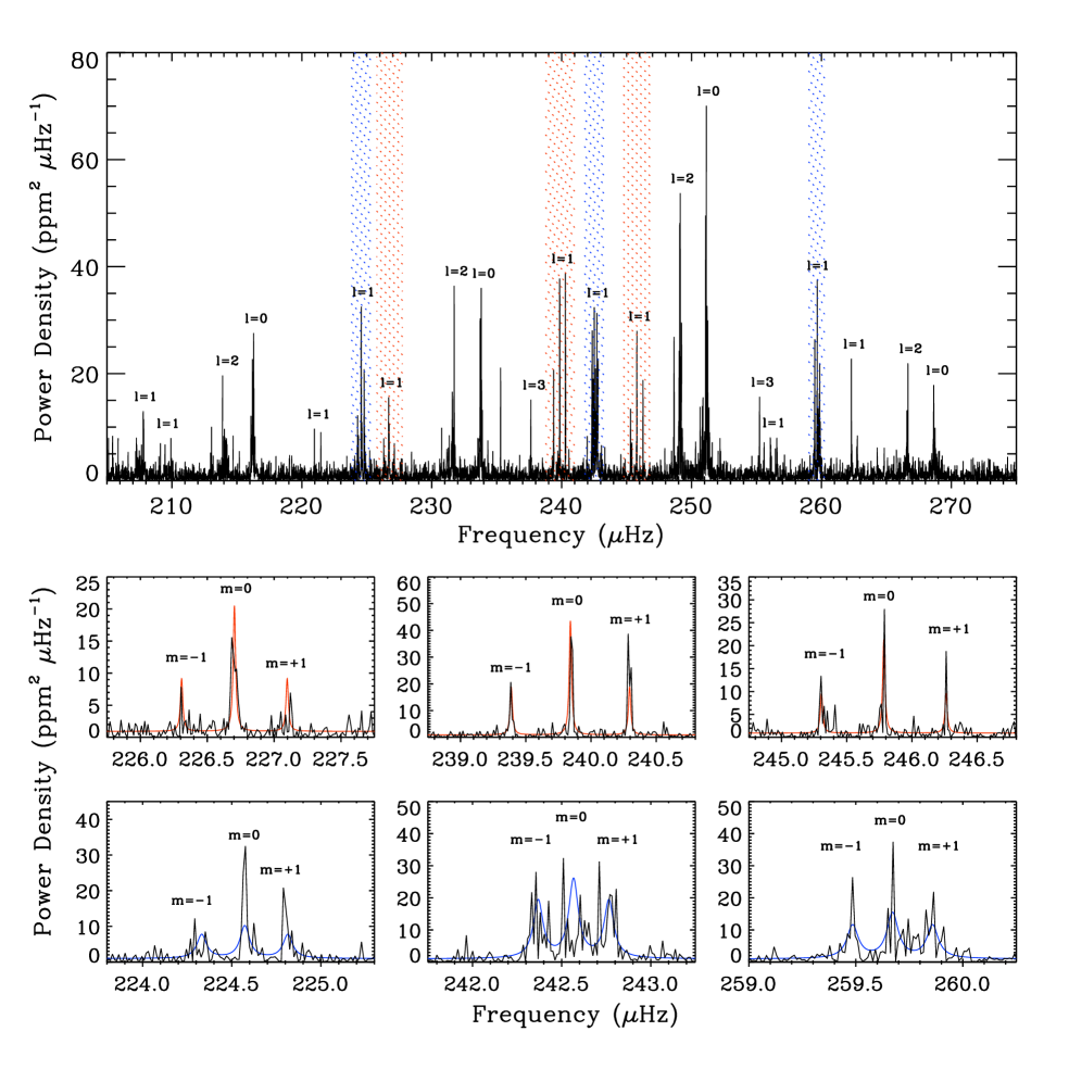
Transit observations lead to measurements of planet properties relative to stellar properties, and hence accurate knowledge of the host star is required to characterize the system. Asteroseismology enables inference of stellar properties through the measurement of oscillations excited by near-surface convection (?). The power spectrum of the Kepler-56 data after removing the planetary transits shows a regular series of peaks (Fig. 1), which are characteristic of stellar oscillations. By combining the measured oscillation frequencies with the effective temperature and chemical composition obtained from spectroscopy, we were able to precisely determine the properties of the host star  (?). Kepler-56 is more than four times as large as the Sun and its mass is 30% greater (Table 1).

Non-radial oscillations in evolved stars are mixed modes, behaving like pressure modes in the envelope and like gravity modes in the core (?, ?). Unlike pressure-dominated mixed modes, gravity-dominated mixed modes have frequencies that are shifted from the regular asymptotic spacing. Mixed modes are also approximately equally spaced in period  (?). We measured the average period spacing between dipole ($l=1$) modes in Kepler-56 to be $50$ seconds, consistent with a first ascent red giant (?).

Individual mixed dipole modes are further split into multiplets as a result of stellar rotation. Because the modes in each multiplet are on average expected to be excited to very nearly equal amplitudes, the observed relative amplitudes depend only on viewing angle relative to the stellar rotation axis (?). For Kepler-56  several mixed dipole modes show triplets (Fig. 1). A rotation axis perpendicular to the line of sight (inclination $i=90^{\circ}$) would have produced a frequency doublet, whereas a star viewed pole-on ($i=0^{\circ}$) would have produced no visible splitting  (?). Therefore the observed triplets are a clear signature of an intermediate inclination of the stellar rotation axis with respect to the line of sight. This also implies an intermediate inclination with respect to the planetary orbital axes, which are known to be perpendicular to the line of sight from the existence of transits.

For a quantitative measurement of the stellar spin-axis inclination, we modeled the six dipole modes with the highest signal-to-noise values. The fitted parameters included the frequency, height, width, rotational splitting and inclination for each mode. Three fitted modes (Fig. 1, middle panels) correspond to gravity-dominated mixed modes, whereas the other three multiplets (Fig. 1, bottom panels) are pressure-dominated mixed modes. The best fitting model yields an inclination angle $i_{\rm g}=43\pm 4^{\circ}$ for gravity-dominated modes and $i_{\rm p}=51\pm 4^{\circ}$ for pressure-dominated modes. Simulations confirmed that the inclination measurements are not strongly affected by the stochastic excitation of the oscillation modes, and both inclinations are consistent with the coarser determination that can be made from estimates of the spectroscopic projected rotational velocity and the surface rotation rate  (?). Furthermore, the measured splittings for gravity-dominated mixed modes are substantially higher than for pressure-dominated mixed modes, consistent with internal differential rotation in red-giant stars (?). Our observations thus reveal that Kepler-56 rotates differentially with a rapidly spinning core, and that both the core and the envelope are (within 1.4-$\sigma$) mutually aligned and inclined by about 45^∘ to the line of sight of the observer.

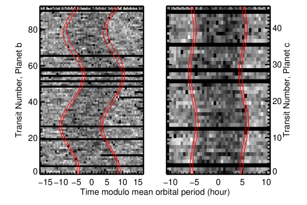
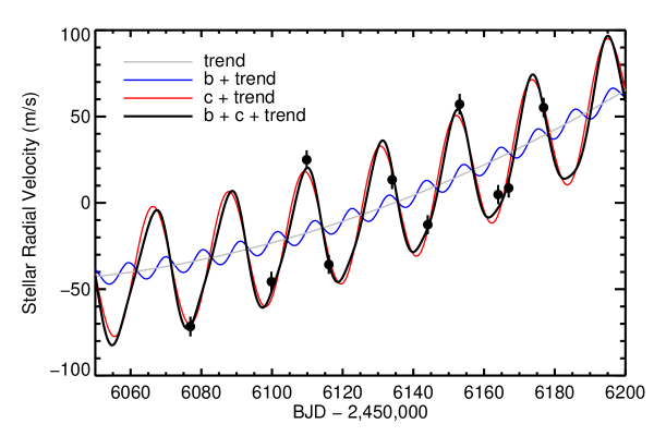
To measure the properties and orbital parameters of the planets, we used the stellar properties from asteroseismology to fit a model to the Kepler data that includes gravitational interactions between the planets, as revealed in the transit time variations (a “photodynamical” model; Fig. 2). In addition to the Kepler light curves, we obtained 10 high-precision radial velocity measurements using the HIgh-Resolution Echelle Spectrometer (HIRES) at the Keck 10-m telescope. The radial velocities show the Doppler signal of the transiting planets, as well as a slow velocity drift indicating a third, more massive companion in a wide orbit (Fig. 3). The combined fit of transit time variations and radial velocity data yields precise properties of the system (Table 1). Both planets have densities consistent with gas-giant planets, and their radii are comparable to the radius of Jupiter $R_{\rm J}$ for planet c ($R=0.88\pm 0.04R_{\rm J}$) and intermediate between Saturn and Neptune for planet b ($R=0.58\pm 0.03R_{\rm J}$). The planets are more than 30% larger than previously thought (?), because asteroseismology enables a more accurate measurement of the host star’s properties.

Further analysis also shows that the orbits of the planets are nearly circular and co-planar. By itself the pattern of transit time variations does not imply coplanar orbits, but in combination with the radial velocity data the mutual inclination is required to be either very low ($\lesssim 10^{\circ}$) or moderately high ($\gtrsim 60^{\circ}$)  (?). We performed dynamical stability simulations using initial conditions drawn from the posterior distribution of the photodynamical model. The highly inclined solutions were dynamically unstable on a timescale of $10^{4}$ years  (?). Thus, the transiting planets in the Kepler-56 system are on co-planar orbits that are misaligned with the equatorial plane of the host star.

Several theories have been proposed to explain stellar spin-orbit misalignments. Favored scenarios include dynamical perturbations such as Kozai cycles (?) and planet-planet scattering (?). These scenarios would be consistent with the presence of a third companion, but would tend to randomize mutual inclinations of planets (and therefore lead to mutually inclined multi-planet systems) unless the perturbations occurred early enough for the inclinations to be damped by the protoplanetary disk. Alternative tilting mechanisms invoke interactions of the stellar magnetic field with the proto-planetary disc (?), angular momentum transport within the star by internal gravity waves (?), or tidal interactions in the early stages of star formation (?). These theories are consistent with a co-planar multi-planet system, but do not require the presence of a third companion on a wide orbit. Spin-orbit misalignments could also be produced through a scenario involving torques from nearby planets or companion stars in inclined orbits (?, ?). Contrary to other scenarios, such a mechanism would naturally produce both a co-planar multi-planet system and a third companion in a wide orbit, as observed for Kepler-56.

The wide companion in the Kepler-56 system thus offers an intriguing explanation for the misalignment based on a scenario originally proposed for the transiting multi-planet system HAT-P-13 (?). The radial velocity drift implies a third companion with the mass of a gas-giant planet within a few astronomical units, or a brown dwarf or star within several dozen astronomical units. In either case, if the third companion’s orbit is itself inclined with respect to the inner planetary orbits (for example through planet-planet scattering, if the companion is a planet), it could have torqued the orbits of the inner planets out of the equatorial plane of the host star. The inner planetary orbits would stay aligned with one another because of strong coupling between their orbits, resulting in a misalignment of the two co-planar transiting planets with the host star. Dynamical simulations that include a third companion in an eccentric orbit inclined to the equatorial plane of the host star confirm that such a mechanism can reproduce the architecture of the Kepler-56 system  (?).

Obliquity measurements have long been considered as a powerful tool to test planet formation theories (?, ?). In particular, observations of the Rossiter-McLaughlin effect have revealed that stars hosting hot Jupiters (mass $\gtrsim 0.3$ times the mass of Jupiter, period $<10$ days) show a wide range of obliquities (?, ?, ?, ?). This finding has been interpreted as supporting evidence for dynamical perturbations as the origin of hot Jupiters, and against scenarios in which hot Jupiters migrate inward because of an interaction with the protoplanetary disk (?). This conclusion, however, relies on the assumption that the stellar equator is a good tracer of the initial orbital plane of the planet (and hence the protoplanetary disk), which has previously been called into question (?, ?). Important test cases are co-planar multi-planet systems which, if primordial alignments are common, should predominantly show low obliquities. Indeed, until now all transiting multi-planet systems have been found to be well-aligned (?, ?, ?).

Although our observations do not constrain the primordial inclination of the protoplanetary disk of Kepler-56, they provide firm evidence that stellar spin-orbit misalignments are not solely confined to hot-Jupiter systems. Continued radial velocity measurements will reveal whether the third companion in the Kepler-56 system is a planet (implying that the initial misalignment occurred after the planets formed) or a star (implying a primordial misalignment of the protoplanetary disk).

Acknowledgements: We gratefully acknowledge the entire Kepler team for making this paper possible. Funding for the Kepler Mission is provided by NASA’s Science Mission Directorate. We thank E. Agol and D. Raggozine for helpful comments on the manuscript. Supported by an appointment to the NASA Postdoctoral Program at Ames Research Center, administered by Oak Ridge Associated Universities through a contract with NASA (D.H.); a NSF Graduate Research Fellowship (K.M.D.); a NSF Graduate Research Fellowship under grant DGE‐1144469 (B.T.M.); the Netherlands Organisation for Scientific Research (S.H.); BELSPO for contract PRODEX COROT (J.M.); the NASA Kepler Participating Scientist program (R.S.-O., J.N.W. and E.B.F.); NSF grant AST-1105930 (S.B.); and the David and Lucile Packard and Alfred P. Sloan foundations (J.A.J.); J.A.C. is a Hubble Fellow of the Harvard-Smithsonian Center for Astrophysics. Funding for the Stellar Astrophysics Centre is provided by Danish National Research Foundation grant DNRF106. The research is supported by the ASTERISK (ASTERoseismic Investigations with SONG and Kepler) project funded by the European Research Council (grant agreement 267864).

Host Star
Radius ($R_{\odot}$)	$4.23\pm 0.15$
Mass ($M_{\odot}$)	$1.32\pm 0.13$
Mean Density (g cm-3)	$0.0246\pm 0.0006$
log [Surface gravity] (cgs)	$3.31\pm 0.01$
Effective Temperature (K)	$4840\pm 97$
Metallicity [M/H] (dex)	$0.20\pm 0.16$
Age (Gyr)	$3.5\pm 1.3$
Stellar Inclination (degrees)	$47\pm 6$
Planet b
Time of Transit (BJD)	$2454978.2556^{+0.0056}_{-0.0057}$
Orbital Period (days)	$10.5016^{+0.0011}_{-0.0010}$
Semi-major axis (AU)	$0.1028^{+0.0037}_{-0.0037}$
Radius ($R_{\oplus}$)	$6.51^{+0.29}_{-0.28}$
Mass ($M_{\oplus}$)	$22.1^{+3.9}_{-3.6}$
Mean Density (g cm-3)	$0.442^{+0.080}_{-0.072}$
Planet c
Time of Transit (BJD)	$2454978.6560^{+0.0057}_{-0.0055}$
Orbital Period (days)	$21.40239^{+0.00059}_{-0.00062}$
Semi-major axis (AU)	$0.1652^{+0.0059}_{-0.0059}$
Radius ($R_{\oplus}$)	$9.80^{+0.46}_{-0.46}$
Mass ($M_{\oplus}$)	$181^{+21}_{-19}$
Mean Density (g cm-3)	$1.06^{+0.14}_{-0.13}$

Table 1: Properties of the Kepler-56 system. Host star properties were derived using asteroseismology and high-resolution spectroscopy. The inclination angle was calculated as a weighted average of the inclination measured from gravity-dominated and pressure-dominated dipole modes, and includes uncertainties from finite mode lifetimes  (?). Because the orbits are not periodic, orbital periods and transit times for the planets refer to values at an arbitrary reference epoch [barycentric Julian Date (BJD) 2,454,970 BJD]. The mutual orbital inclination of the two planets is $5^{+3.4}_{-3.1}$ degrees at this epoch.

Figure 1: Power spectrum analysis to measure the inclination of the stellar rotation axis. Top panel: Power spectrum centered on the frequency range with excited oscillations. The spherical degree $l$ of each identified mode is indicated. Red and blue areas highlight gravity-dominated and pressure-dominated mixed dipole modes, respectively. Bottom panels: Zoom on the mixed dipole modes highlighted in the top panel. Each mode is split into a triplet by rotation. The azimuthal order $m$ of each component is indicated. Red and blue lines show the modeled Lorentzian profiles. The scatter in the data about the fitted model is due to the finite mode lifetimes  (?).

Figure 2: Transit time variations of the inner planets. Stellar intensity is plotted as a function of transit epoch and time modulo the mean orbital period near transits of planet b (left) and c (right). The red lines mark the 68% confidence intervals for the start and end of each transit, according to the photodynamical model.

Figure 3: Radial velocity variations. Solid circles show the individual radial velocity measurements as a function of barycentric Julian date; the black solid line is the best-fitting photodynamical model to the combined Kepler and radial velocity data. Thin gray, blue and red lines show the individual components of the fit, which includes a radial velocity drift modeled as a quadratic function of time and radial velocity variations due to planet b and c. The drift is attributed to a third, massive companion in a wide orbit.

Supplementary Materials

1 Asteroseismic Data Analysis

1.1 Observations and Data Preparation

The asteroseismic analysis is based on Kepler long-cadence data (?) collected during Quarters 0–11, spanning a total of 977.8 days. We have used Kepler simple aperture photometry (SAP) for our analysis. Intensity differences between quarters were removed by fitting and correcting a linear regression to 10 day light curve segments before and after each quarterly gap. To correct remaining long-periodic instrumental trends, a quadratic Savitzky-Golay filter (?) with a width of 2 days was applied.

The sharp structure of transits in the time series can cause significant power leakage from low to high frequencies in the power spectrum, and hence they need to be corrected or removed prior to the asteroseismic analysis. Using the average ephemeris and orbital periods identified by the Kepler planet search pipeline (?), we removed data during transits from the time series. To account for transit timing variations, we used transit durations inflated to 19.5 hours for planet b and 16.3 hours for planet c to remove transits from the phase-folded light curve. Note that we have also repeated the analysis by discarding the transits according to the transit timings of the photodynamical model (§5), but found no significant difference in the results.

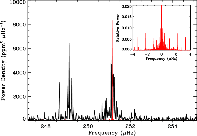
The removal of transits causes a reduction in duty cycle by $\sim$10%. Figure S1 shows the power spectrum of Kepler-56, with the spectral window after removing the transits overlaid on the oscillation mode with the highest power. The spectral window (red) has sidelobes which are below 1% in power, and hence make a negligible contribution to the power spectrum compared to the noise level. We conclude that the removal of transits has no significant impact on the results of the asteroseismic analysis.

Figure S1: A small part of the power spectrum of Kepler-56 (black line), centered on the strongest oscillation mode. The red line shows the spectral window of the timeseries with transits removed, scaled to the frequency and maximum value of the highest peak. The inset shows a close up of the spectral window, with the same $x$-axis range as the main panel and normalized to a height of 1. The sidelobes caused by the periodic transit removal are much lower than the overall noise level and hence negligible for the asteroseismic analysis.

1.2 Extraction of Oscillation Parameters and Frequencies

To extract oscillation parameters characterizing the average properties of the power spectrum, we used automated analysis methods (?, ?) which have been thoroughly tested on Kepler data of other stars (?, ?). In brief, the power contribution due to granulation noise and stellar activity was modeled by a combination of power laws, and then corrected by dividing the power spectrum by the background model. Next, the frequency of maximum power ($\nu_{\rm max}$) was measured by heavily smoothing the power spectrum or by fitting a Gaussian function to the power excess. Finally, the large frequency separation ($\Delta\nu$), i.e. the average separation of modes with the same spherical degree and consecutive radial order, was determined by computing an autocorrelation of the power spectrum or of the time series, and identifying the most significant peak. The high S/N of the Kepler-56 data allowed a very precise determination of both quantities, yielding $\mbox{$\nu_{\rm max}$}=244.3\pm 1.4\,\mbox{$\mu$Hz}$ and $\mbox{$\Delta\nu$}=17.4\pm 0.1\,\mbox{$\mu$Hz}$.

To extract individual oscillation frequencies we first smoothed the background-corrected power spectrum with a Gaussian function with a FWHM of 1$\mu$Hz. The spectrum was then manually inspected for peaks significantly above the noise level (S/N $>$ 4), and for each identified mode a power-weighted centroid was calculated. To estimate uncertainties, Monte-Carlo simulations were performed by perturbing the power spectrum with random numbers drawn from a $\chi^{2}$ distribution with two degrees of freedom. For each iteration, the power weighted centroids were recalculated, and the uncertainty for each frequency was taken as the standard deviation of the resulting distribution. In an alternative approach, a statistical test was employed to identify frequencies with low probabilities of being due to noise  (?). These frequencies were manually inspected and additional frequencies were selected if appropriate. The power spectrum was then fitted using a global fit, with the frequency, width and height as free parameters for each mode. The fitting was based on a maximum likelihood estimation and uncertainties were computed from the Hessian matrix. Finally, the uncertainties on the determined frequencies obtained using the methods described above were checked by performing a Markov-Chain Monte-Carlo analysis to fit a global model to the power spectrum  (?).

$f(\mbox{$\mu$Hz})$	$\sigma_{f}(\mbox{$\mu$Hz})$	$l$	$m$	$f(\mbox{$\mu$Hz})$	$\sigma_{f}(\mbox{$\mu$Hz})$	$l$	$m$
190.525	0.023	1	–	237.624	0.017	3	0
192.402	0.029	1	–	239.380	0.007	1	$-1$
196.888	0.019	2	0	239.848	0.007	1	0
198.985	0.017	0	0	240.296	0.006	1	$+1$
205.113	0.011	1	$-1$	242.363	0.011	1	$-1$
205.437	0.009	1	0	242.566	0.015	1	0
205.869	0.013	1	$+1$	242.749	0.013	1	$+1$
207.730	0.025	1	0	245.326	0.011	1	$-1$
209.055	0.018	1	$-1$	245.779	0.008	1	0
209.463	0.011	1	0	246.278	0.012	1	$+1$
209.996	0.018	1	$+1$	249.135	0.017	2	0
214.017	0.025	2	0	251.150	0.016	0	0
216.237	0.016	0	0	255.204	0.017	3	0
220.965	0.011	1	$-1$	255.571	0.024	1	$-1$
221.464	0.012	1	0	256.086	0.017	1	0
221.926	0.011	1	$+1$	256.534	0.016	1	$+1$
224.312	0.012	1	$-1$	259.486	0.009	1	$-1$
224.582	0.007	1	0	259.687	0.011	1	0
224.809	0.009	1	$+1$	259.842	0.011	1	$+1$
226.340	0.013	1	$-1$	262.303	0.014	1	–
226.699	0.007	1	0	262.746	0.015	1	–
227.088	0.013	1	$+1$	266.617	0.019	2	0
231.654	0.019	2	0	268.683	0.020	0	0
233.760	0.015	0	0	277.538	0.024	1	0
213.035	0.022	–	–	235.307	0.020	–	–
230.777	0.022	–	–	248.651	0.017	–	–

Table S1: Measured oscillation frequencies for Kepler-56. The spherical degree $l$ and azimuthal order $m$ is indicated for each frequency. Frequencies in the bottom two rows correspond to significant peaks for which no clear mode identification could be determined.

Figure S2: Échelle diagram of the background corrected power spectrum. Darker regions mark frequencies with higher power. Open symbols show extracted frequencies with spherical degrees $l=0$ (blue squares), $l=1$ (red diamonds), $l=2$ (green triangles) and $l=3$ (magenta asterisks). Note that for the extracted frequencies we have plotted the central frequency of each order on the vertical axis  (?), and that the plot is duplicated past the vertical dashed line for clarity.

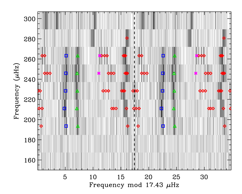
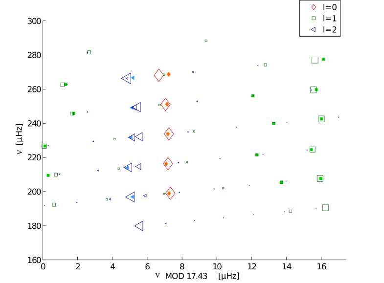
Figure S2 shows an échelle diagram, which is calculated by plotting the power spectrum modulo the large frequency separation (hence stacking orders of equal spherical degree on top of each other). Oscillation modes with spherical degree $l=0,1,2$ and 3 are denoted by green triangles, blue squares, red diamonds and magenta asterisks. The vertical ridge along which oscillation modes line up in the échelle diagram is much broader for $l=1$ modes than for $l=0$ and 2 modes, due to the presence of mixed modes  (?). Four orders contain $l=1$ modes with clear triplet structure due to rotational splitting  (?, ?, ?), which allows for an identification of the azimuthal degree $m$. The extracted frequencies including a mode identification are listed in Table S1.

Figure S3: Comparison of power spectra calculated from Q0-11 long-cadence data (black) and Q9-11 short-cadence data (red). Note that the y-axis for the latter has been inverted for clarity. The vertical dotted line marks the long-cadence Nyquist limit. Both power spectra are nearly indistinguishable, showing that Nyquist effects are negligible when using long-cadence data for the asteroseismic analysis.

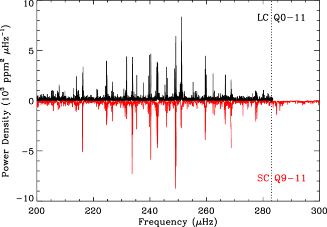
The proximity of the power excess to the long-cadence Nyquist limit (283$\mu$Hz) raises some concern about the effect of reflection of power at the Nyquist frequency on the extracted parameters, in particular for the determination of $\nu_{\rm max}$. Although Q9-11 short-cadence data are available for Kepler-56, the four-times-higher frequency resolution in long-cadence data is essential for resolving the rotationally split multiplets. To test the influence of Nyquist effects, Figure S3 compares the power spectrum using long-cadence data to a power spectrum calculated using the Q9-11 short-cadence data. The comparison shows that there are no significant reflection effects in the long-cadence data and that, except for a few low-amplitude modes at the highest frequencies, all frequencies are well captured. A re-determination of $\nu_{\rm max}$ and $\Delta\nu$ using short-cadence data yielded nearly identical to those obtained using long-cadence data, but with higher uncertainties. This confirms that the extracted oscillation parameters and individual frequencies using long-cadence data were not affected by Nyquist effects.

1.3 Host Star Inclination

1.3.1 Power Spectrum Modeling

The inclination of a rotating star can be determined by measuring the relative heights of rotationally split oscillation modes  (?, ?, ?). To measure the inclination of Kepler-56, we fit rotationally split Lorentzian profiles to the six strongest triplets of dipole modes in the power spectrum (see Figure 1). The model power $P$ as a function of frequency $\nu$ can be described as:

$$P(\nu)=\sum_{k=1}^{N}\sum_{m=-l}^{+l}\frac{\epsilon_{lm}(i)h_{k}}{1+4(\nu-f_{k}-ms_{k})^{2}\Gamma^{-2}}+n\>.$$ (1)

Here, $h$ is the mode height, $f$ is the central mode frequency, $\Gamma$ is the mode linewidth, $s$ is the rotational splitting, and $n$ is an arbitrary noise floor in the power spectrum. The outer sum runs over the $N$ oscillation modes to be fitted, while the inner sum runs over the azimuthal order $m$ of each frequency. The relative height of each component is given by $\epsilon_{lm}(i)$, which depends on the azimuthal order $m$, spherical degree $l$ and inclination angle $i$. For dipole modes ($l=1$), $\epsilon_{lm}(i)$ can be written as  (?):

$$\epsilon_{l=1,~{}m=0}=\cos^{2}i\>,$$ (2)

$$\epsilon_{l=1,~{}m\pm 1}=\frac{1}{2}\sin^{2}i\>.$$ (3)

Note that this formulation assumes that the intrinsic mode height is independent of $m$. The amplitudes of the $m=\pm 1$ components relative to the $m=0$ component then give a direct measure of the stellar inclination, independent of effects such as the Coriolis force or stellar limb darkening  (?). According to Equations (2) and (3) observations of frequency triplets can be used to immediately rule out edge-on or pole-on inclinations of the stellar spin axis.

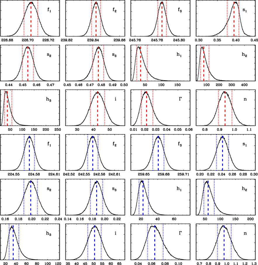
We performed two fits, once using three gravity-dominated $l=1$ modes, and once using three pressure-dominated $l=1$ modes (see Figure 1). The power spectrum was first corrected for background contributions due to activity and granulation, as described in the previous section. For each mode, we fitted the central frequency $f$, rotational splitting $s$ and mode height $h$. The inclination $i$, linewidth $\Gamma$ and noise floor $n$ were assumed to be the equal for each set of three modes, yielding a total of 12 free parameters. The fit was performed using a Markov-Chain Monte-Carlo algorithm. The likelihood function $\mathcal{L}$ for fitting a power spectrum is given by $\chi^{2}$ statistics with two degrees of freedom and hence can be written as  (?, ?, ?):

$$\mathcal{L}=\prod_{\nu}\frac{1}{P_{\rm m}(\nu)}\exp\left(-\frac{P_{\rm o}(\nu)}{P_{\rm m}(\nu)}\right)\>.$$ (4)

Here, $P_{\rm m}(\nu)$ is the power predicted by the model at a frequency $\nu$, and $P_{\rm o}(\nu)$ is the observed power. For the priors $p$ we assume Jeffreys priors for the mode heights:

$${p(x)}=\frac{1}{x\ln({\frac{x_{\rm max}}{x_{\rm min}}})}\>,$$ (5)

and uniform priors for the remaining parameters:

$${p(x)}=\frac{1}{x_{\rm max}-x_{\rm min}}\>.$$ (6)

Here, $x_{\rm min}$ and $x_{\rm max}$ are the minimum and maximum allowed values for a given parameter $x$. We performed $5\times 10^{6}$ iterations, and discarded the first 5% of each chain. The best-fitting values and uncertainties were calculated as the median and 84.1 and 15.9 percentile of the marginalized posterior distribution for each parameter. Table S2 reports these values, and Figure S4 shows the posterior distributions for each set of fitted gravity- and pressure-dominated $l=1$ modes. We have checked the results by sub-dividing the time series into two parts of equal length, and repeating the power spectrum analysis on these two independent datasets. The derived inclinations agreed well (within $6^{\circ}$ for p-dominated and g-dominated modes) with the results derived from the full dataset.

We note that the rotational splittings of gravity-dominated dipole modes are on average twice as large as the splittings measured from pressure-dominated dipole modes, consistent with other red giants observed by Kepler  (?, ?).

Parameter	g-dominated modes	p-dominated modes
$f_{1}(\mbox{$\mu$Hz})$	$226.7030^{+0.0066}_{-0.0069}$	$224.5730^{+0.0077}_{-0.0076}$
$f_{2}(\mbox{$\mu$Hz})$	$239.8421^{+0.0034}_{-0.0034}$	$242.5669^{+0.0103}_{-0.0101}$
$f_{3}(\mbox{$\mu$Hz})$	$245.7844^{+0.0040}_{-0.0038}$	$259.6717^{+0.0086}_{-0.0084}$
$s_{1}(\mbox{$\mu$Hz})$	$0.395^{+0.013}_{-0.018}$	$0.242^{+0.011}_{-0.011}$
$s_{2}(\mbox{$\mu$Hz})$	$0.4534^{+0.0040}_{-0.0039}$	$0.198^{+0.010}_{-0.010}$
$s_{3}(\mbox{$\mu$Hz})$	$0.4773^{+0.0046}_{-0.0050}$	$0.187^{+0.010}_{-0.010}$
$h_{1}$	$36.0^{+20.6}_{-12.1}$	$22.3^{+6.6}_{-4.8}$
$h_{2}$	$78.3^{+41.4}_{-24.5}$	$59.9^{+20.3}_{-14.2}$
$h_{3}$	$37.5^{+19.0}_{-11.7}$	$34.4^{+10.7}_{-7.8}$
$i$ (deg)	$42.5^{+4.4}_{-4.3}$	$50.5^{+3.9}_{-4.0}$
$\Gamma(\mbox{$\mu$Hz})$	$0.0217^{+0.0056}_{-0.0048}$	$0.065^{+0.012}_{-0.011}$
$n$	$0.936^{+0.047}_{-0.045}$	$0.971^{+0.078}_{-0.073}$

Table S2: Results of fitting rotationally split Lorentzian profiles to two sets of three mixed $l=1$ modes. Fitted parameters are the central frequency $f$, the rotational splitting $s$, the mode height $h$, the inclination $i$, the linewidth $\Gamma$ and the noise floor $n$. Note that $h$ and $n$ are dimensionless quantities measured relative to the background. The quoted values are the median as well as 84.1% and 15.9% confidence intervals.

Figure S4: Posterior distributions of the MCMC analysis of three gravity-dominated and three pressure-dominated rotationally-split dipole modes in the Kepler-56 power spectrum. Annotations in each panel follow the description of each parameter listed in Table S2. Dashed lines show the median and dotted lines the 84.1% and 15.9% confidence intervals, respectively. The three top rows show the posteriors for gravity-dominated modes (red lines) and the three bottom rows show the posteriors for pressure-dominated modes (blue lines).

1.3.2 Finite Mode Lifetime Simulations

It is important to examine how our measurement of the stellar inclination is affected by the finite lifetimes of the oscillation modes. Solar-like oscillations are stochastically excited and damped  (?, ?), with mode lifetimes ranging from a few days for main-sequence stars to several weeks or months for cool red giants  (?, ?, ?, ?, ?, ?). The main effect of stochastic excitation is that solar-like oscillations are not described by a sinc function in the Fourier domain, but rather by a series of peaks modulated by a Lorentzian profile whose width depends on the lifetime of the modes. If the Lorentzian profile is not well resolved (i.e. the observation timebase is not much greater than the mode lifetime), the observed peaks will vary in height, depending on the time of observation.

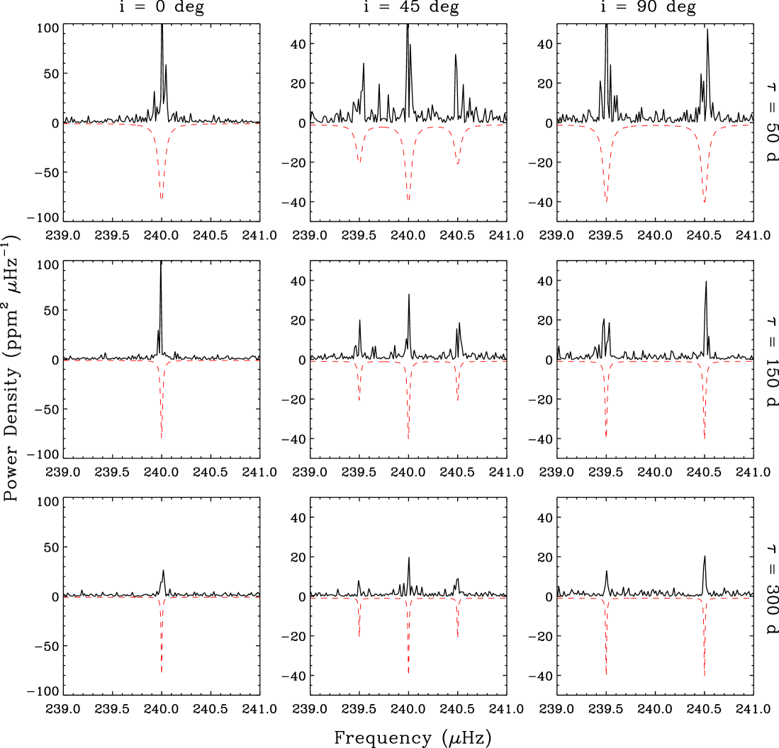
The maximum mode lifetime for Kepler-56, based on the fit of Lorentzian profiles, is about 170 days, indicating that the modes are not well-resolved by the observational timebase of 998 days. To ensure that our measured inclination from the relative mode heights of rotationally split multiplets is not biased by finite mode lifetimes, we performed simulations as follows. Using the timestamps of the original Kepler-56 observations, we generated synthetic timeseries by simulating a damped, harmonic oscillator with a given frequency, amplitude and mode lifetime  (?). The frequency and height of the simulated mode were set to typical values observed in Kepler-56  and we added shot noise corresponding to the observed Kepler data. To simulate a rotationally split mode we added two additional modes spaced by an equal amount in frequency, and fixed the relative mode heights to the central mode for a given input inclination. Figure S5 shows several examples for synthetic power spectra over a range of mode lifetimes and inclinations for a single simulated mode in Kepler-56. A comparison with the underlying input models, shown in red, illustrates the effect of the finite mode lifetimes on the resulting spectrum.

We performed 2000 simulations by drawing random input values for inclinations and mode lifetimes from uniform distributions in the ranges 0–90 degrees and 30–300 days, and generating three rotationally split modes with typical frequencies and mode heights as observed in Kepler-56. For one half of the simulations we used a rotational splitting typical for pressure-dominated modes in Kepler-56, and for the other half we used rotational splittings typical for gravity-dominated modes. For each simulation, we performed the same MCMC analysis as applied to the real data. Figure S6 shows the determined inclinations compared to the input values, as well a histogram of the differences between output and input values. The results demonstrate that there is no bias introduced by finite mode lifetimes on the determination of the stellar inclination, and that inclinations are securely recovered for a wide range of input parameters. The residuals show a standard deviation of 5 degrees, in very good agreement with our estimated uncertainties for the original data. To account for finite mode lifetimes, we add in quadrature the scatter from our simulations to the uncertainty of the weighted average inclination from pressure- and gravity-dominated modes, yielding our final stellar inclination measurement for Kepler-56 of $i=47\pm 6^{\circ}$.

1.3.3 Three-Dimensional Stellar Spin-Orbit Angle

The three-dimensional angle $\psi$ between the stellar spin axis and the planetary orbital axes is given as  (?):

$$\cos\psi=\sin i\cos\lambda\sin i_{0}+\cos i\cos i_{0}\>,$$ (7)

where $\lambda$ is the sky-projected stellar spin-orbit angle, and $i_{0}$ is the angle between the line of sight and the orbital axis of the planet. The angle $\lambda$ can be measured through spectroscopic observations of the Rossiter-McLaughlin effect or observations of planet - starspot crossings, but remains unconstrained in the asteroseismic analysis. If $i$ and $i_{0}$ are known, a lower limit of $\psi$ can be calculated:

$$\cos\psi<\sin i\sin i_{0}+\cos i\cos i_{0}\>.$$ (8)

Using the values for $i$ and $i_{0}$ derived from our asteroseismic and photo-dynamical analysis, we calculate $\psi>37^{\circ}$ for Kepler-56. For low eccentricity orbits, the lower limit on $\psi$ can be approximated as follows  (?):

$$\cos\psi\lesssim\sin i+\frac{R_{\rm s}}{a_{\rm p}}\cos i\>.$$ (9)

Here, $R_{\rm s}$ is the stellar radius and $a_{\rm p}$ is the semi-major axis of the planet. Equation (9) illustrates that a large value of $i$ (i.e., the stellar rotation axis being nearly perpendicular to the line of sight) for a transiting system does not necessarily imply a stellar spin-orbit alignment, while a small value for $i$ always implies a stellar spin-orbit misalignment.

Figure S5: Simulations illustrating the influence of inclination and mode lifetime on observed power spectra. In each panel, red dashed lines show the input model and black lines show the calculated power spectrum of the simulated Kepler-56 timeseries. Note that the input models have been inverted for clarity. Mode frequencies, heights, and input shot noise were set to typical values for observations of Kepler-56. The stochastic excitation of the modes causes the observed spectrum to scatter around the input spectrum. Note that only intermediate inclinations produce a distinct set of triplets, as observed for Kepler-56 (see Equations (2) and (3)).

Figure S6: Simulation results to validate the measured inclination of Kepler-56. The top two panels show the input mode lifetime and input inclination versus the difference between the output and input inclination. Note that the sharp edges in the middle panel are caused by the condition that the output inclination is measured between 0 and 90 degrees. The bottom panel shows a histogram of the differences between output and input inclination. The residual scatter over all mode lifetimes is $5^{\circ}$.

2 Surface Rotation and Stellar Inclination from Starspots

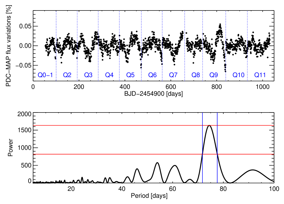
Stars like Kepler-56 can have starspots that are carried across their surfaces by stellar rotation, which produces quasi-periodic flux variations. This variability was filtered out in order to study the stellar pulsations, which occur on much shorter timescales. However, rotational modulation due to spots can be used to measure the surface rotation rate and even to constrain the stellar inclination. Kepler simple aperture photometry (SAP) data cannot be used for this purpose because of artificial flux changes due to pointing drifts and other systematic effects  (?). We therefore used the corrected flux series processed with the PDC-MAP algorithm  (?, ?) to estimate the rotation period. This algorithm finds the systematic trends using a selected group of stars in each CCD module and uses that information to correct the light curves of all Kepler stars. The final product should mainly preserve the astrophysical sources of variability. We applied a 3-sigma clipping algorithm to the PDC-MAP data with a 12 hour-long moving-median filter, and also normalized each quarter by its median. The final flux series is shown in the upper panel of Figure S7, where the data have been binned to two points per day. Quasi-periodic variability of the order of $0.05-0.1$% can be observed, with a period that does not seem to be strongly correlated with the quarter duration.

We calculated a Lomb-Scargle periodogram and found a clear peak around 75 days (lower panel, Figure S7). This periodicity can be seen also in the time series data. We interpret this periodicity as the signal introduced by spots rotating across the stellar disk. In the Lomb-Scargle periodogram we find the range of periods where the power is higher than half the peak power. This range is adopted as the 1-$\sigma$ uncertainties, and the center of the interval is the final value of the surface rotation period  (?). With this prescription, we find a rotation period of $74\pm 3$ days, which corresponds to a frequency of $0.156\pm 0.006\mbox{$\mu$Hz}$. Combined with the rotational splitting of pressure and gravity dominated dipole modes, these observations show that the star rotates more slowly on the surface than within the interior of the star  (?, ?, ?). Using the radius of the star and the $v\sin i$ obtained from spectroscopy (§3.1) we obtain an independent value of the stellar inclination of $i_{\rm s}=36\pm 25^{\circ}$, in agreement with the asteroseismic analysis. While the agreement is reassuring, the precision of the $v\sin i$-based method is comparatively poor, and the accuracy of the method is also questionable due to the difficulties of measuring $v\sin i$ values as small as the one observed for Kepler-56 (see §3.1). Furthermore, the determined rotation period is close to the length of Kepler observing quarters and hence may be affected instrumental effects such as flux discontinuities between quarter boundaries.

Figure S7: Quasi-periodic flux variations induced by starspots and rotation are used to obtain a surface rotation period and to check the stellar inclination. Upper panel: The mean-normalized mean-subtracted PDC-MAP flux series is represented with black dots. The data are binned to show only two points per day. Each quarter is labeled in blue to show that the stellar variability is not strongly correlated with the quarter boundaries. Lower panel: A Lomb-Scargle periodogram of the flux series shows a clear peak at 74 days, which we interpret as the surface rotation period. The red and blue lines mark the full-width at half-maximum of that peak.

3 Host Star Properties

3.1 Atmospheric Parameters

We obtained spectroscopic follow-up observations of Kepler-56 using the Fiber-fed Échelle Spectrograph (FIES) on the 2.5 m Nordic Optical Telescope (NOT) on La Palma, Spain  (?). Three spectra were acquired in July 2011 with a resolution of R = 67,000 and an individual exposure time of 60 minutes yielding an average signal-to-noise ratio per resolution element of 47 in the MgB region. The stellar parameters were derived using the Stellar Parameter Classification pipeline (SPC)  (?). In an initial analysis, effective temperature, surface gravity and metallicity were fit simultaneously to match the spectrum to a library of synthetic spectra. In a second iteration, the surface gravity was fixed to a value of $\mbox{$\log g$}=3.29$, as determined from the asteroseismic gridmodeling analysis (see next section). This procedure was adopted to minimize potential correlations between Teff, log(g) and metallicity  (?), and yielded final parameters of $\mbox{$T_{\rm eff}$}=4840\pm 97$ K, $\mbox{$\rm{[M/H]}$}=+0.20\pm 0.16$ dex and $v\sin i=1.7\pm 1.0$ km s^-1. To account for systematic differences between different spectroscopic methods, the quoted uncertainties include contributions of 59 K, 0.062 dex and 0.85 km s^-1 in $T_{\rm eff}$, $\rm{[M/H]}$ and $v\sin i$, respectively, which were added in quadrature to the formal uncertainties  (?).

3.2 Asteroseismic Grid-Modeling

In a first step to estimate stellar properties using asteroseismology, we have used the asteroseismic observables $\nu_{\rm max}$ (the frequency of maximum power) and $\Delta\nu$ (the average separation between modes of the same spherical degree and consecutive radial order). It can be shown that $\nu_{\rm max}$ and $\Delta\nu$ are approximately related to stellar properties as follows  (?, ?, ?):

$$\Delta\nu\approx\frac{({M/M_{\odot}})^{1/2}}{(R/R_{\odot})^{3/2}}\Delta\nu_{\odot}\>,$$ (10)

$$\nu_{\rm max}\approx\frac{M/M_{\odot}}{(R/R_{\odot})^{2}\sqrt{T_{\rm eff}/T_{\rm eff,\odot}}}\nu_{\rm max,\odot}\>.$$ (11)

Given an estimate of $T_{\rm eff}$, Equations (10) and (11) can be solved to obtain radius and mass, in the so-called direct method  (?, ?). Alternatively, $\Delta\nu$ and $\nu_{\rm max}$ can be used in combination with evolutionary tracks, spectroscopic temperatures and metallicities to estimate stellar properties  (?, ?, ?). Equations (10) and (11) have been tested observationally using eclipsing binary systems, Hipparcos parallaxes, and long-baseline interferometry  (?, ?, ?), and have also been supported theoretically  (?, ?). For evolved stars, Equations (10) and (11) have generally been found to yield radii and masses accurate to 5% and 10%, respectively  (?, ?).

To derive fundamental properties, we have employed the grid-based method to match the spectroscopic and asteroseismic parameters to a variety of evolutionary tracks  (?, ?, ?, ?, ?). The solar reference parameters used were $\mbox{$\nu_{\rm max}$}=3090\,\mbox{$\mu$Hz}$ and $\mbox{$\Delta\nu$}=135.1\,\mbox{$\mu$Hz}$  (?). We note that the recently proposed revision of Equation (10)  (?) has negligible influence on our results, and that the stellar properties derived from scaling relations are only used as an input for a more detailed analysis using individual oscillation frequencies (see next section) and to reduce degeneracies in the spectroscopic analysis (see previous section).

3.3 Individual Frequency Modeling

We have used the ATON code  (?) to compute a grid of stellar interior models with masses in the range $1.26-1.56$ $M_{\odot}$ in steps of $0.02\,\mbox{$M_{\odot}$}$, helium mass fractions of $Y=0.27-0.33$ in steps of 0.01, metal mass fractions of $Z=0.028-0.030$ in steps of 0.001 and mixing length parameters $\alpha_{\rm MLT}=1.9,2.05$ and $2.2$. For each track we computed adiabatic oscillation frequencies using LOSC  (?, ?) for all models having a large frequency separation within 10% of the observed value.

Model frequencies were corrected for near-surface effects  (?). The power-law correction was applied to both radial and non-radial frequencies. Since the latter may have inertias considerably different to those of radial modes, the surface correction for non-radial modes was multiplied by $Q_{n,l}^{-1}$, where $Q_{nl}$ is the ratio of the mode inertia of the mode to that of the closest radial mode  (?). To explore uncertainties in the exponent $b$ describing the power-law correction we considered $b=3,6$, and $8$. To match the model frequencies to the observed frequencies we evaluated the reduced $\chi^{2}$ for the frequencies and the spectroscopic constraints separately. For the best matching models, the contribution of the spectroscopic constraints to the reduced $\chi^{2}$ is typically lower than 1.

Figure S8 shows an échelle diagram of the best-fit model compared to the observed frequencies. The match of both radial and non-radial frequencies to the observations is very good, and in particular reproduces the mixed dipole modes. We note that our best-fit models indicate that the trapping between the pressure-mode and gravity-mode cavities is strong enough for some $l=2$ mixed modes to have relatively low inertias, and therefore possibly excited to observable amplitudes. Some of the additional modes with no clear identification (see Table S1) may be compatible with mixed $l=2$ modes.

The properties of the best-fitting model are $M=1.32\pm 0.13\,M_{\odot}$, $R=4.23\pm 0.15\,R_{\odot}$ and $\rho=0.0246\pm 0.0006$ g cm^-3, with an age of $3.5\pm 1.3$ Gyr. The helium mass fraction, iron mass fraction and mixing length parameter of the best-fitting model are $Y=0.29$, $Z=0.03$, and $\alpha_{\rm MLT}=2.2$. Fully consistent results were derived with an independent analysis using ASTEC models  (?, ?, ?). Uncertainties on the properties were estimated by adopting the fractional uncertainties of the grid-based method described in the previous section. These estimates encompass the properties of best-fit models obtained by fitting individual frequencies and making different assumptions on the surface-correction term (see above). Importantly, we note that the mean stellar density derived using individual model frequencies is 5% higher than the density derived using Equation (10) ($\rho=0.0234\pm 0.0003$ g cm^-3). This result has been confirmed using other techniques to model individual frequencies, and is in-line with previous studies showing deviations of Equation (10) from models for evolved stars  (?, ?).

Figure S8: Échelle diagram comparing the observed frequencies (filled symbols) with theoretical frequencies of the best-fitting model (open symbols). Modes of different spherical degree are shown as diamonds ($l=0$), squares ($l=1$) and triangles ($l=2$). The size of the open symbols is inversely proportional to $E^{1/2}$, where $E$ is the mode inertia  (?). Note that rotationally split components ($m\neq 0$) are not included in the merit function and hence are not plotted in the diagram.

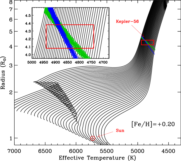
To illustrate the evolutionary state of Kepler-56, Figure S9 shows evolutionary tracks from the BaSTI database  (?) for the measured metallicity of Kepler-56, quadratically interpolated to a fine grid in stellar mass. The red box shows the position of Kepler-56 as determined from the asteroseismic analysis of individual frequencies and spectroscopic follow-up. Additionally, green and blue models highlight the 1-$\sigma$ constraints from $\Delta\nu$ and $\nu_{\rm max}$, as used in the previous section.

Figure S9: BaSTI evolutionary tracks for a metallicity of [Fe/H] = 0.20 and masses ranging from 0.9 to 1.6 solar masses with a stepsize of 0.02. Models fullfilling 1-$\sigma$ observational constraints for the large frequency separation $\Delta\nu$ (green) and the frequency of maximum power $\nu_{\rm max}$ (blue) are highlighted in the plot. Red lines show the 1-$\sigma$ error box in radius and temperature derived from asteroseismic modeling of individual frequencies and the spectroscopic analysis with asteroseismic constraints. The position of the Sun is shown in the bottom part of the plot. The inset shows a close-up of the position of Kepler-56.

4 Radial Velocity Data

We obtained spectroscopic observations of Kepler-56 at Keck Observatory (Mauna Kea, Hawaii) using the HIgh-Resolution Echelle Spectrometer (HIRES)  (?) with the standard observational setup used by the California Planet Survey  (?). All observations were made with an iodine cell mounted directly in front of the spectrometer entrance slit. The iodine absorption lines observed with the stellar spectrum provide a precise wavelength scale to measure Doppler shifts and place constraints on the shape of the HIRES instrumental profile at each observing epoch  (?).

Because of the star’s relative faintness ($m_{\rm V}=12.8$) we used the C2 decker, corresponding to a sky-projected size of $14\mbox{$.\!\!^{\prime\prime}$}0$ by $0\mbox{$.\!\!^{\prime\prime}$}851$. The increased height of the C2 decker, compared to the shorter B5 decker normally used for brighter stars, allows for sky subtraction and provides a resolving power of $R=\lambda/\Delta\lambda\approx$ 55,000. We obtained a total of 10 observations with exposure times ranging from 750 to 1800 seconds, resulting in signal-to-noise ratios between 50 and 90 at 550 nm.

In each observation, we determined the radial velocity of Kepler-56 relative to a “template” observation of the star with its instrumental profile removed through deconvolution. Two templates were collected of the star, each without the presence of iodine in the light path. The same decker was used for the templates as for the other observations. The radial velocity measurements, times of observation, and internal uncertainties are listed in Table S3.

JD $-$ 244000	RV (m s-1)	Unc. (m s-1)	SNR
16076.904083	-71.6087	2.4468	62
16099.840740	-45.5976	2.4815	62
16109.824833	24.9774	1.7344	88
16116.089211	-35.6964	1.5950	89
16133.999602	13.4154	1.6138	89
16144.079281	-12.6180	1.9468	84
16153.086751	57.1263	2.9634	52
16163.980793	4.8418	1.8606	89
16166.962497	8.5878	1.7946	89
16176.855891	55.1829	2.1804	65

Table S3: Radial velocities for Kepler-56. The uncertainties reported in the third column are formal measurement uncertainties and do not include the effects of stellar chromospheric “jitter” on our observations.

5 Photodynamical Modeling

The times of transit of the two planets are not strictly periodic owing to planet-planet dynamical interactions. These deviations may be interpreted to infer bulk and orbital properties including, for example, a combination of planetary mass and orbital eccentricity, or, the mutual inclination between the planetary orbits (the stellar density from asteroseismology also helps to constrain the vectorial eccentricity component $e\sin\omega$ for each orbit, where $e$ is the eccentricity and $\omega$ the argument of periastron). However, the transit times are difficult to estimate at individual epochs owing to correlated noise in excess of the photon noise. To attempt to resolve this, we fit all transit events simultaneously assuming a physically accurate model. This model includes dynamical interactions and an accurate description of the photometric noise.

In detail, the light curve and radial velocity of Kepler-56 were modeled using a dynamical simulation to determine the motions of the planets and star and a transit light curve model to predict the light curve at the observed times. In addition to this deterministic model, an extended noise model was fitted to account for the significant time-correlated stellar granulation signal superposed with Poisson photon noise. The posterior distribution of the model parameters was sampled using a Markov chain Monte Carlo algorithm. The details of this model, its application, and the derived results are described in this section.

5.1 Preparation of the Light Curve Data

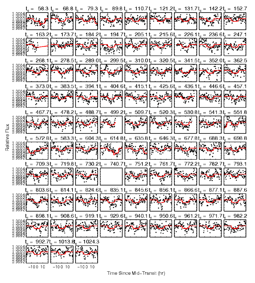
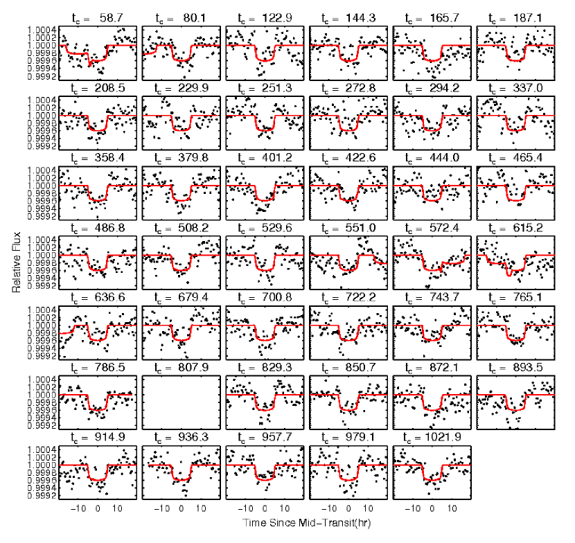
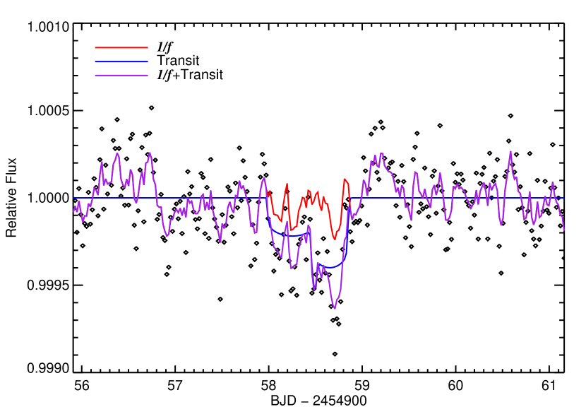
We isolated the observations near the planetary transit events in the full Kepler light curve (specifically “SAP_FLUX”) for Kepler-56. We retain 96 continuous segments of 256 cadences (roughly 5.2 days) centered on single transit events or, when transits of both planets occur within 5.2 days of one another, centered halfway between two transits. We choose 256 cadences — a power of 2 — to facilitate the rapid computation of the wavelet transform when computing the likelihood (see §5.4). Figures S10, S11 show a portion of the data utilized in our analysis, within $\sim 1$ day of a transit event.

A quadratic trend in time was fitted to each continuous segment and divided through the data. The parameters of this quadratic trend were found iteratively, re-estimated after fitting the data with the photometric-dynamical model using a nonlinear fitter (Levenberg-Marquardt). At each iteration step, the best-fitting light curve model and correlated noise model were removed from the data and the quadratic trend was refit to the residuals; the revised trend was divided through the data and the process was repeated until the parameters of the trend converged to sufficient tolerance.

Figure S10: Light curve data and best-fitting transit model (in red) near transits of planet b. Times of transit less $2,454,900$ BJD are indicated above each plot cell. Note that empty panels are due to data gaps in the Kepler time series.

Figure S11: Light curve data and best-fitting transit model (in red) near transits of planet c. Times of transit less $2,454,900$ BJD are indicated above each plot cell. Note that empty panels are due to data gaps in the Kepler time series.

5.2 Dynamical Simulation

We perform a dynamical integration to determine the positions and velocities of all three bodies in Kepler-56 at any time. This integration utilized a Jacobian coordinate system  (?). In this system, ${\bf r_{b}}$ is the position of planet b relative to the star, and ${\bf r_{c}}$ is the position of planet c relative to the center of mass of planet b and the star. These coordinates and masses are specified (via the parameterization described in §5.5) at some fiducial time to uniquely specify the evolutionary history over our observations.

The computations are performed in a Cartesian system, although it is convenient to express ${\bf r_{b}}$ and ${\bf r_{c}}$ and their time derivatives in terms of osculating Keplerian orbital elements: instantaneous period, eccentricity, argument of pericenter, inclination, longitude of the ascending node, and time of transit. We denote these quantities as $P_{b,c}$, $e_{b,c}$, $\omega_{b,c}$, $i_{b,c}$, $\Omega_{b,c}$, and $T_{b,c}$, respectively. We note that these parameters do not necessarily reflect observables in the light curve; the unique three-body effects make these parameters functions of time. The “time of transit,” in particular, refers to the modeled time of transit at the reference epoch; it cannot be used in conjunction with the modeled orbital period to compute a simple ephemeris for the system, due to transit timing variations.

The accelerations of the three bodies are determined from Newton’s equations of motion, which depend on ${\bf r_{b}}$, ${\bf r_{c}}$ and the masses  (?, ?). For the purpose of reporting the masses and radii in Solar units, we assumed $G\mbox{$M_{\odot}$}=2.959122\times 10^{-4}$ AU³ day^-2 and $\mbox{$R_{\odot}$}=0.00465116$ AU. We used a Bulirsch-Stoer algorithm  (?) to integrate the coupled first-order differential equations for $\dot{\bf r}_{b,c}$ and ${\bf r}_{b,c}$. We set a positional accuracy of $10^{-16}$ AU. The positions and velocities determined from the dynamical simulation were then used as input to a light curve model.

5.3 Light Curve Model

We did not determine the spatial coordinates of all three bodies at each observed time in the Kepler light curve. Instead, to speed computation, we recorded for each epoch only the sky-plane projected separation between star and planet, and the sky-plane projected speed of planet relative to star at the calculated time of transit. The times of transit were determined numerically by minimizing the projected separation between the star and planet. The result of these calculations was a collection of transit times $t^{k}_{i_{k}}$, impact parameters $b^{k}_{i_{k}}$ and speeds $v^{k}_{i_{k}}$ for each planet $k\in\{b,c\}$ and for epochs $i_{k}\in N_{k}$ where $N_{k}$ is the set of observed epoch numbers for planet $k$. The motion of the planet relative to the star is approximately linear in the sky-plane such that the projected separation as a function of time is, to good approximation,

$$Z^{k}_{i_{k}}(t)=\sqrt{\left[v^{k}_{i_{k}}(t-t^{k}_{i_{k}})\right]^{2}+\left(b^{k}_{i_{k}}\right)^{2}}$$ (12)

for times near (a few transit durations) of the calculated mid-transit time.

The approximate photometric model for the relative stellar flux, $f(t)$, is then defined as

$$f(t)=1-\sum_{k}\sum_{i_{k}\in N_{k}}\left\{\begin{array}[]{ll}\lambda\left(Z^{k}_{i_{k}}(t),R^{k},u\right)&-0.5\leq t-t^{k}_{i_{k}}\leq 0.5\\ 0&{\rm otherwise}\end{array}\right.$$ (15)

where $\lambda(z,r,u)$ is the overlap integral between a limb darkened star of radius $R_{\star}$ (such that the radial brightness profile is $I(\rho/R_{\star})/I(0)=1-u[1-\sqrt{1-(\rho/R_{\star})^{2}}]$ with linear limb-darkening parameter $u$) whose center is separated by a distance $z$ from a dark, opaque sphere of radius $r$. $\lambda(z,r,u)$ may be computed semi-analytically with available codes  (?). This photometric model, assuming constant transit velocity, is faster to compute than calculating the positions at each photometric cadence and results in a negligible change in the quality of the model fit to the data compared to exact integration. This model does not include the “anomalous” brightening events that occur when the planet c occults planet b during a transit  (?). No such events are observed, nor are they predicted to occur, within the current dataset.

The continuous model $f(t)$ is integrated over a 29.4 min interval centered on each long cadence sample using a Gaussian-quadrature integration with 10 samples per cadence.

5.4 Photometric Noise Model

Investigation of the Kepler light curve shows a significant correlated stochastic signal in addition to the coherent oscillations (utilized in the asteroseismic analysis) and the transit events (see Figure S12). This signal is attributed to stellar granulation, is approximately stationary (i.e., temporal correlation depends only on relative separations in time), and has a power spectral density that scales inversely with frequency. This nearly $1/f$ (“pink”) power spectral density is typical of granulation noise  (?, ?, ?). This correlated noise can significantly bias parameters related to the transit events (e.g., mid-transit times, depths) if not properly accounted for  (?).

In response, we model the photometric noise, $\eta$, as $\eta(t)=\epsilon+\gamma(t)$ where $\epsilon$ and $\gamma$ are both normally distributed [$\epsilon\sim{\cal N}(0;\Sigma_{w})$, $\gamma\sim{\cal N}(0;\Sigma_{p})$], $\epsilon$ is uncorrelated “white” noise, and $\gamma$ is correlated “pink” noise. To facilitate the rapid computation of this model and its associated likelihood, we use the wavelet-based formalism described in Carter & Winn (2009)  (?). Here, the data $\eta(t)$ (or the data residuals after removing the transit model, $\eta(t)=F(t)-f(t)$) are projected into components $\hat{\eta}_{m,n}$ of a wavelet basis (indexed by scale $m$ and position $n$). In this basis, the covariance of the components is approximately diagonal

$$\langle\hat{\eta}_{m,n}\hat{\eta}_{m^{\prime},n^{\prime}}\rangle \approx (\sigma_{r}^{2}2^{-m}+\sigma_{w}^{2})\delta_{m,m^{\prime}}\delta_{n,n^{\prime}}$$ (16)

where we have parameterized the noise model by two parameters, $\sigma_{w}^{2}$ and $\sigma_{r}^{2}$. The first parameter is the variance of $\epsilon$ (associated with photon-noise only) while the second parameter is related to the scale of the correlated noise component.

Figure S12: Example decomposition of single data segment into its constitute components: transit model (blue; itself the superposition of a nearly simultaneous transits of Planets b and c) and a stochastic correlated noise component (red).

5.5 Specification of Parameters

The reference epoch of the initial conditions was chosen to be $t_{0}=2,454,950$ (BJD). The photo-dynamical model has 23 adjustable parameters. Two parameters are related to stellar constraints from asteroseismology: the stellar density times the gravitational constant, $G\rho_{\star}$, and the stellar radius, $R_{\star}$. Two parameters are the mass ratios $q_{+}\equiv(M_{b}+M_{c})/M_{\star}$ and $q_{p}\equiv M_{b}/M_{c}$. Four parameters are combinations of the eccentricities $e_{b,c}$ and arguments of pericenter $\omega_{b,c}$ in a nonlinear way, chosen to give nearly linear correlations between their uncertainties (and thereby avoid the computational cost often associated with nonlinear correlations):

$$h_{-} \equiv (P_{b}/P_{c})^{2/3}e_{b}\cos\omega_{b}-e_{c}\cos\omega_{c}$$ (17)

$$h_{+} \equiv (P_{b}/P_{c})^{2/3}e_{b}\cos\omega_{b}+e_{c}\cos\omega_{c}$$ (18)

$$k_{-} \equiv (P_{b}/P_{c})^{2/3}e_{b}\sin\omega_{b}-e_{c}\sin\omega_{c}$$ (19)

$$k_{+} \equiv (P_{b}/P_{c})^{2/3}e_{b}\sin\omega_{b}+e_{c}\sin\omega_{c}$$ (20)

The remaining osculating parameters, 7 in total, are the periods $P_{b}$, $P_{c}$, the orbital inclinations $i_{b}$, $i_{c}$, the times of transit $T_{b}$, $T_{c}$ and the difference between the nodal longitudes $\Delta\Omega\equiv\Omega_{c}-\Omega_{b}$.

Two more parameters are the relative radii of the planets: $r_{b}\equiv R_{b}/R_{\star}$ and $r_{c}\equiv R_{c}/R_{\star}$. One parameter, $u$, parameterizes the linear limb darkening law for the star.

Two parameters, $\sigma_{w}^{2}$ and $\sigma_{r}^{2}$, characterize the extended noise model (see § 5.4).

The remaining parameters parameterize the radial velocity model: 3 describe the quadratic trend and one parameter gives the additional stellar jitter ($\sigma_{\rm jitter}$), added in quadrature to the formal velocity errors.

5.6 Model Likelihood and Priors

We adopted uniform priors in the parameters described in the previous section excluding $h_{+,-}$ and $k_{+,-}$. For these latter four parameters, we enforced uniform priors in eccentricities and arguments of pericenter. For these priors, the probability density obeys

$$p(h_{+,-},k_{+,-})dh_{+,-}k_{+,-} \propto p(e_{b,c},\omega_{b,c})\times\frac{1}{e_{b}e_{c}}d_{e_{b},e_{c}}d_{\omega_{b},\omega_{c}}\propto\frac{1}{e_{b}e_{c}}d_{e_{b},e_{c}}d_{\omega_{b},\omega_{c}}$$ (21)

The likelihood ${\cal L}$ of a given set of parameters was taken to be the product of likelihoods based on the photometric data (each 256 cadence segment projected into a discrete fourth-order Daubechies wavelet basis), the assumed-Gaussian asteroseismology priors and the radial velocity data:

$${\cal L} \propto \prod^{{\rm segments}}\left[\prod_{n}\prod_{m}(\sigma_{r}^{2}2^{-m}+\sigma_{w}^{2})^{-\frac{1}{2}}\exp\left(-\frac{1}{2}\frac{\hat{\eta}^{s}_{m,n}}{\sigma_{r}^{2}2^{-m}+\sigma_{w}^{2}}\right)\right]$$

$$\times\prod_{i}(\sigma_{i}^{2}+\sigma_{\rm jitter}^{2})^{-\frac{1}{2}}\exp\left(-\frac{1}{2}\frac{\Delta RV_{i}^{2}}{\sigma_{i}^{2}+\sigma_{\rm jitter}^{2}}\right)\times$$

$$\times\exp\left[-\frac{1}{2}\left(\frac{\Delta G\rho_{\star}}{\sigma_{G\rho_{\star}}}\right)^{2}\right]\times\exp\left[-\frac{1}{2}\left(\frac{\Delta R_{\star}}{\sigma_{R_{\star}}}\right)^{2}\right]$$

where $\hat{\eta}^{s}_{m,n}$ are the wavelet components of the $s$th segment photometric residuals after removing the transit model $f(t)$ (see Carter & Winn 2009 for additional details), $\Delta RV_{i}$ is the residual of the $i$th radial velocity measurement with formal error $\sigma_{i}$, and $\Delta G\rho_{\star}/\sigma_{G\rho_{\star}}$ and $\Delta R_{\star}/\sigma_{R_{\star}}$ are the deviates between the asteroseismic constraints in density and radius.

5.7 Parameter Estimation

We explored the parameter space and estimated the posterior parameter distribution with a Differential Evolution Markov Chain Monte Carlo (DE-MCMC) algorithm  (?). We generated a population of 60 chains and evolved through approximately 500,000 generations. The initial parameter states of the 60 chains were randomly selected from an over-dispersed region in parameter space bounding the final posterior distribution. The first 10% of the links in each individual Markov chain were clipped, and the resulting chains were concatenated to form a single Markov chain, after having confirmed that each chain had converged according to the standard criteria including the Gelman-Rubin convergence statistics and the observation of a long effective chain length in each parameter (as determined from the chain autocorrelation).

5.8 Photodynamical Modeling Results

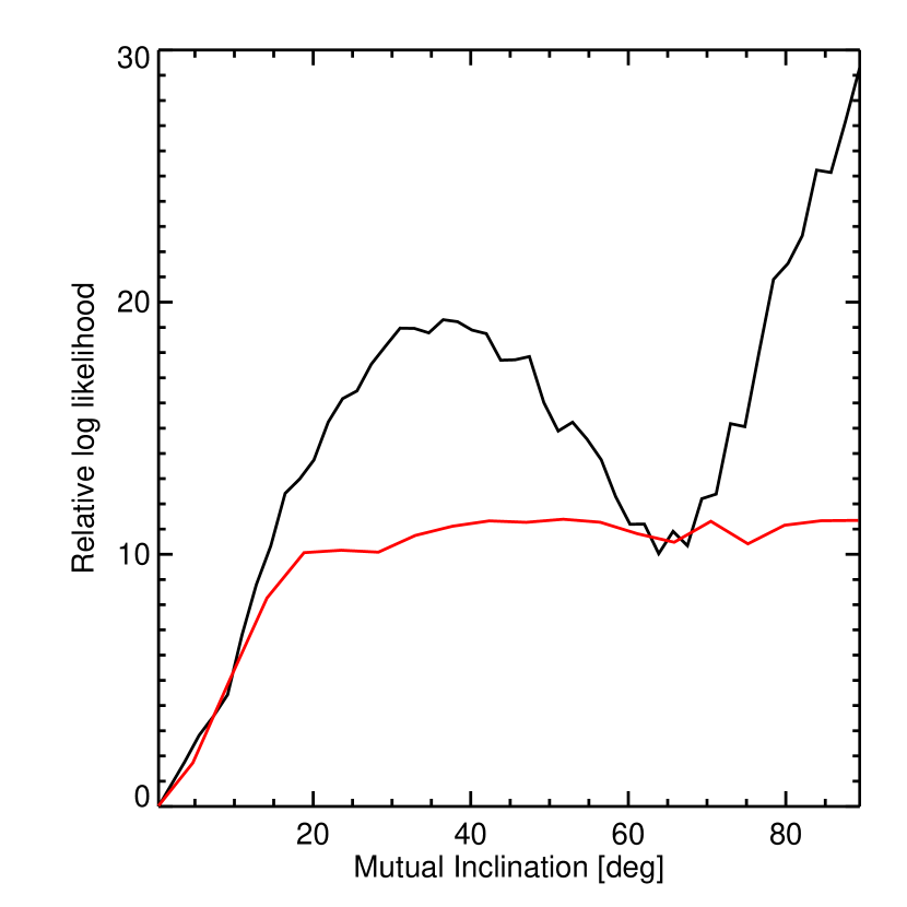
Initially, we included only the photometric data subject to the asteroseismic constraints on stellar density and radius in our analysis, excluding the radial velocity data. Examining the MCMC results, we found that at low mutual orbital inclination $I$, defined such that

$$\cos I = \sin i_{b}\sin i_{c}\cos\Delta\Omega+\cos i_{c}\cos i_{b},$$ (23)

the planetary orbits were nearly circular and the planetary masses were moderately constrained (to within $\approx$10%).

Arbitrarily high mutual inclinations are marginally consistent (Figure S13) with the photometric data (in the tail of the posterior distribution) so long as the planetary masses, orbital eccentricities and arguments of periapse are relatively fine-tuned. These dependences are shown in Figure S14. The source of these curious correlations is the changing character of the transit timing anomalies at mutual inclinations exceeding roughly 20 degrees.

Figure S13: Relative log-likelihood as a function of mutual inclination estimated from the photo-dynamical model when RV data is excluded (red) or included (black). Smaller values correspond to higher likelihood.

Figure S14: Best-fitting parameters as a function of the relative nodal longitude between the orbits of Planet b and c, fitting only the photometric data (subject to the constraints from asteroseismology). The shaded gray regions indicate the 1$\sigma$ intervals of uncertainty. The best-fitting architecture undergoes a finely-tuned “phase change” for mutual inclinations (approximately equal to the relative nodal longitude) greater than 20^∘.

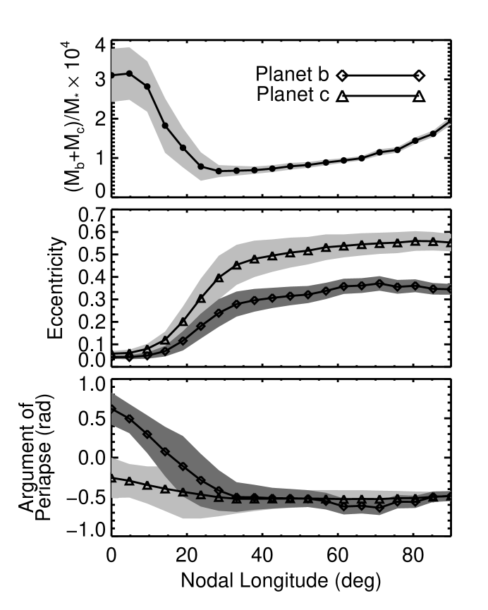
At low mutual inclinations, the periodicity of the timing anomaly is determined by the period of the longitude of conjunction, defined as the mutual anomaly at planetary conjunction  (?, ?): $P_{\rm LOC}=|2/P_{c}-1/P_{b}|^{-1}$. At high inclinations, additional minima in separation appear near conjunctions at either node (orbital plane crossings) and occur twice each $P_{\rm LOC}$. As a result, a frequency doubled component arises in the TTV at high inclinations (see Figure S15). The onset of this frequency doubling occurs at moderate mutual inclinations.

Figure S15: Transit timing variation for Kepler-56 b and c as a function of mutual inclination keeping all other parameters fixed.

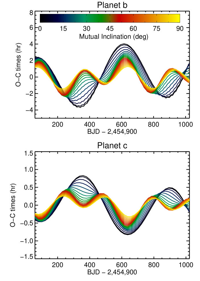
The data favor a single periodicity (see Figure 2) at the expected period $P_{\rm LOC}\approx 590$ days  (?). However, by carefully orienting the orbits and increasing eccentricities (and finely tuning their masses to keep the TTV amplitude constant), the frequency doubled component can be suppressed. In particular, when pericenters are aligned and the eccentricity is sufficiently large the longitude of conjunction sweeps quickly through the line of nodes; in this case, the behavior of the TTV is approximately described with a single component. This is demonstrated in the correlations shown in Figure S14 for mutual inclinations $I>20$ degrees; these high eccentricity solutions have approximately equal likelihoods, slightly lower than low inclination solutions (see Figure S13).

The inclusion of the radial velocity data in our analysis resolved this degeneracy between mutual inclination and planet mass sum or orbital eccentricity. In detail, the radial velocity data constrained both the planetary masses and the eccentricity of their orbits to a range consistent with low mutual inclination. Moderate mutual inclinations ($15^{\circ}<I<50^{\circ}$) and high mutual inclinations ($I>75^{\circ}$) were excluded by the data. A lower likelihood connected region near $I\approx 60^{\circ}$ was statistically plausible (Figure S13), but was ultimately excluded based on considerations of long-term dynamical stability (see §6). We conclude that the orbits are coplanar to within $I<10^{\circ}$ at 95% confidence (Figure S16).

Figure S16: Distribution of mutual inclination, $I$, determined from the photometric-dynamical analysis (solid line) and the prior for $I$ (dotted line). Both distributions have been normalized so that the maximum equals unity.

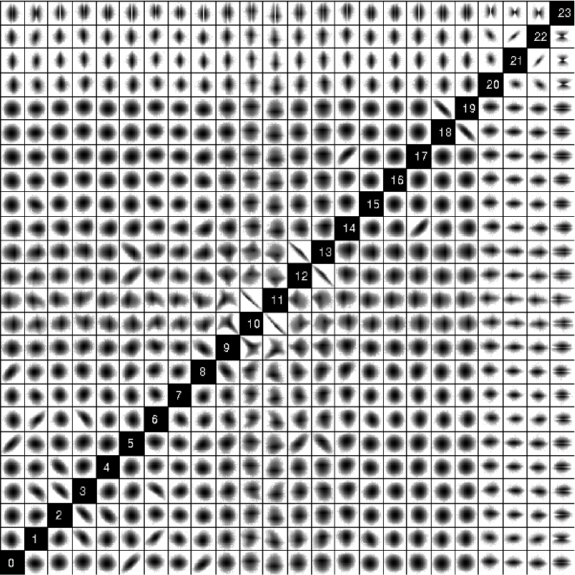
Table 5.8 provides the best-fitting photometric-dynamical model parameters, their medians and uncertainties (provided as 68% confidence intervals of the marginalized parameter posterior drawn by the MCMC algorithm). Table 5.8 provides a number of derived parameters. Figure S17 shows 2D joint probability distribution plots between the fitted parameters (and references the parameter indices listed in Table 5.8). These plots are meant to qualitatively display the correlations amongst the parameters.

Index	Parameter Name	Best-fit	50%	15.8%	84.2%
	Mass parameters
0	Mean Density, $\rho_{\star}$ (g cm-3)	$0.02458$	$0.02461$	$-0.00060$	$+0.00059$
1	Mass sum ratio, $(M_{b}+M_{c})/M_{A}(\times 10^{5})$	$47.7$	$46.8$	$-3.9$	$+3.9$
2	Planetary mass ratio, $M_{b}/M_{c}$	$0.129$	$0.122$	$-0.015$	$+0.015$
	Inner Binary Orbit (Planet b)
3	Orbital Period, $P_{b}$ (day)	$10.51046$	$10.51057$	$-0.0010$	$+0.0011$
4	Time of Transit, $t_{b}$ (days since $t_{0}$)	$8.2581$	$8.2556$	$-0.0057$	$+0.0056$
5	Orbital Inclination, $i_{b}$ (deg)	$83.84$	$83.92$	$-0.25$	$+0.26$
	Outer Binary Orbit (Planet c)
6	Orbital Period, $P_{c}$ (day)	$21.40221$	$21.40239$	$-0.00062$	$+0.00059$
7	Time of Transit, $t_{c}$ (days since $t_{0}$)	$8.6531$	$8.6560$	$-0.0055$	$+0.0057$
8	Orbital Inclination, $i_{c}$ (deg)	$84.02$	$84.08$	$-0.087$	$+0.091$
9	Relative Nodal Longitude, $\Delta\Omega$ (deg)	$-4.91$	$-4.95$	$-3.5$	$+3.8$
	Eccentricity parameters
10	$e_{b}\cos\omega_{b}-(a_{c}/a_{b})e_{c}\cos\omega_{c}$	$0.033$	$0.032$	$-0.022$	$+0.018$
11	$e_{b}\cos\omega_{b}+(a_{c}/a_{b})e_{c}\cos\omega_{c}$	$0.033$	$0.034$	$-0.023$	$+0.032$
12	$e_{b}\sin\omega_{b}-(a_{c}/a_{b})e_{c}\sin\omega_{c}$	$-0.010$	$-0.004$	$-0.013$	$+0.019$
13	$e_{b}\sin\omega_{b}+(a_{c}/a_{b})e_{c}\sin\omega_{c}$	$-0.010$	$-0.020$	$-0.031$	$+0.018$
	Radius Parameters
14	Linear Limb Darkening Parameter, $u$	$0.464$	$0.530$	$-0.100$	$+0.091$
15	Stellar Radius, $R_{\star}$ ($R_{\odot}$)	$4.19$	$4.22$	$-0.15$	$+0.15$
16	b Radius Ratio, $R_{b}/R_{\star}$	$0.01419$	$0.01414$	$-0.00038$	$+0.00037$
17	c Radius Ratio, $R_{c}/R_{\star}$	$0.02109$	$0.02130$	$-0.00065$	$+0.00064$
	Photometric Noise Parameters
18	White Noise paramter, $\sigma_{w}$ ($\times 10^{5}$)	$12.78$	$12.80$	$-0.20$	$+0.19$
19	Pink Noise parameter, $\sigma_{r}$ ($\times 10^{5}$)	$152.3$	$152.5$	$-2.3$	$+2.3$
	RV Parameters
20	RV Offset (m/s)	$13.1$	$13.0$	$-2.6$	$+2.7$
21	Linear Trend (m/s/day)	$0.79$	$0.86$	$-0.12$	$+0.12$
22	Quadratic Trend (m/s/day2)	$0.0017$	$0.0028$	$-0.0025$	$+0.0024$
23	RV Jitter (m/s)	$5.2$	$5.9$	$-1.7$	$+2.8$

Table S4: Photometric-dynamical model parameters. The reference epoch is $t_{0}=$2,454,950 (BJD).

Table S5: Derived parameters. The reference epoch is $t_{0}=$2,454,950 (BJD).

Figure S17: Two-parameter joint posterior distributions of the primary model parameters. The densities are plotted logarithmically in order to elucidate the nature of the parameter correlations. The indices listed along the diagonal indicate which parameter is associated with the corresponding row and column. The parameter name corresponding to a given index is indicated in Table 5.8 in the “Index” column.

6 Dynamical Stability Analysis of the Inner Planets

The photodynamical modeling of the Kepler-56 data results in a posterior joint probability distribution for the model parameters. Marginalizing over all parameters except the radius and density of the star (resulting in the mass of the star), the two mass ratio parameters and the initial positions and velocities of the bodies at a reference epoch results in a posterior distribution for these dynamical parameters. Sets of masses and initial conditions drawn from this distribution are statistically consistent with the photometric and radial velocity data. However, there is no guarantee that these orbits will be stable on longer timescales. We should reject any initial conditions that show instability on timescales much shorter than the age of the system, even if they are consistent with the data, unless there is some reason to believe we are observing the system at a special time.

6.1 Orbital Solutions with High Mutual Inclinations

A set of 6,600 initial conditions, drawn from a Markov chain specially seeded in the region of parameter space corresponding to highly inclined solutions near $I\sim 60^{\circ}$, were tested for dynamical stability. All of these initial conditions failed the Hill stability criterion, implying that crossing orbits and collisions were possible  (?, ?). Although orbits satisfying the Hill criterion can never result in particularly strong gravitational interactions (occurring when the planets pass within a mutual Hill sphere of each other, for example) or direct collisions between the bodies, failing the criterion is not sufficient to conclude that collisions will definitely occur. This is especially true when orbits are protected by a resonance. Hence we cannot immediately conclude that these 6,600 initial conditions are unstable without direct numerical integration.

The dynamical evolution of these initial conditions was studied by evolving the Newtonian equations of motion using a Bulirsch-Stoer integration scheme  (?). No relativistic or dissipative forces were included in these integrations. Energy was conserved in these integrations to within one part in $10^{10}$.

The integrations revealed that the orbits with high mutual inclinations exhibited large amplitude Kozai-like oscillations in the inclinations and eccentricities of the planets. Though the initial eccentricities of the planets are not particularly large ($e_{b}\sim 0.12,e_{c}\sim 0.21$), they correspond to a minimum in the eccentricity oscillations. The maximum eccentricity of the inner planet can approach unity. The eccentricity and sky plane inclination evolution is shown in Figure S18. Throughout this evolution, the semimajor axes are approximately constant, with only a small variation due to coherent oscillations related to the near 2:1 commensurability. Because of this, the large growth in eccentricity directly implies that the minimum pericenter distance of the inner planet becomes very small. When the eccentricity of the inner planet is larger than 0.8, the corresponding pericenter is inside of the host star ($1-e_{b}<R_{\star}/a_{b}=0.2$, where $a_{b}$ is roughly constant). A typical case is shown in Figure S19.

Figure S18: The eccentricity and sky plane inclination evolution of both planets for a randomly chosen initial condition with high mutual inclination.

Figure S19: The pericenter distance of the inner planet is show for the same initial condition as Figure S18. Note that since the bodies are treated as point particles the integrations do not stop when the collision actually occurs.

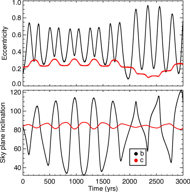
The timescale to reach this critical $e_{b}\approx 0.8$ is shorter for the initial conditions with the highest initial mutual inclination. Over $99\%$ of the initial conditions lead to a collision between the inner planet and the star within $10^{4}$ years. The remaining $1\%$ suffer collisions on timescales of $10^{5}$ years. The distribution of the time required before the inner planet crashes into the star is shown in Figure S20.

Figure S20: The distribution of time required, in years, for the inner planet to reach a pericenter distance inside the surface of the star.

The typical timescales for collisions are very short, and hence tidal damping of eccentricity (or any other dissipative process) would not save the inner planet from this fate unless that dissipation was exceedingly efficient. Additionally, the dynamical effects of a far away perturber would likely be too weak to affect this result, and so we can conclude that the highly mutually inclined orbits which fit the data are unphysical.

6.2 Orbital Solutions with Low Mutual Inclinations

We also studied the short-term stability of solutions with a low initial mutual inclination. Out of $10^{4}$ solutions drawn from the posterior distribution, two failed the Hill criterion. A set of 995 representative low-inclination initial conditions were integrated for $5\times 10^{5}$ years, or $\sim 2\times 10^{7}$ orbits of the inner planet, using a Wisdom-Holman symplectic integrator  (?). Symplectic correctors were implemented to improve the accuracy of the integrations  (?, ?). For these integrations, a relativistic contribution was included because the typical precession rate for the inner planet is on the order of $10^{5}$ years. We used a dipole-like potential, which is straightforward to incorporate into the symplectic integrator, to mimic the effect of general relativity in the weak limit  (?). Energy was conserved to within one part in $10^{10}$. For each of these initial conditions, we kept track of the maximum, minimum and average semi-major axes, eccentricities, pericenters, and sky-plane inclinations of the planets, as well as the mutual inclination of the orbits. The evolution of the eccentricities and sky-plane inclinations for a typical initial condition is shown in Figure S21. The maximum eccentricity reached by the inner planet in any of the integrations was 0.098. Note that the initial eccentricities no longer preferentially correspond to extrema in the secular cycle as was the case for the set of initial conditions with high mutual inclinations. Again, the semi-major axes were approximately constant ($\approx$0.05% variation in $a_{c}$ from the time-averaged value, and $\approx$0.3% variation in $a_{b}$), implying that the inner planet no longer crashes into or even closely approaches the star. The typical pericenter evolution of the inner planet, relative to the radius of the star, is shown in Figure S22. The outer planet had a maximum eccentricity of 0.107, and consequently the orbits do not come close to crossing.

Figure S21: The eccentricity and sky plane inclination evolution of both planets for a typical initial condition with low mutual inclination ($I\sim 5^{\circ}$).

Figure S22: The pericenter distance of the inner planet is show for the same initial condition as Figure S21. Initial conditions with low mutual inclinations do not lead to close approaches between the inner planet and the star.

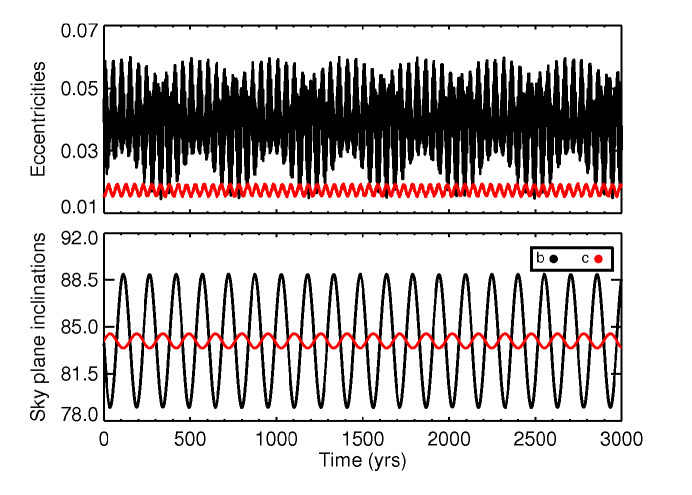
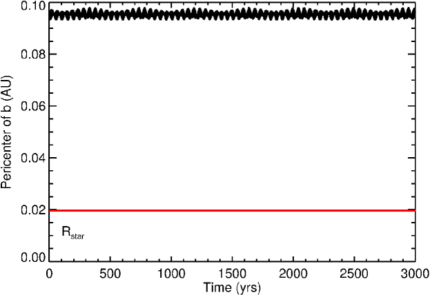
With approximately half of the initial condition studied, corresponding to those orbits with initial mutual inclinations $>$5 degrees, the inner planet periodically stops transiting. The typical timescale for this behavior is 60,000 days (150 years). Similarly, the outer planet stops transiting for about one quarter of the initial conditions, with the same timescale. However, the mean inclinations of the planets over the $5\times 10^{5}$ years always corresponded to impact parameters less than unity. For each initial condition, we monitored the time evolution of the planetary impact parameters. We found that there were 16 initial conditions where only planet c stopped transiting, 281 where only planet b stopped transiting, and 239 where both stopped transiting periodically. This analysis allows us to determine the probability of observing the Kepler 56 system as a different multiplicity system. For example, the probability of seeing the Kepler 56 system as an $n$-transiting system, where $n=0,1,$ or $2$, is $P_{n}=\sum_{\rm allIC}P(IC)f(IC)_{t,n}$, where $P(IC)$ is the probability of the initial condition and $f(IC)_{t,n}$ is the fraction of the integration time that the initial condition spent in an $n$-transiting configuration. Since these initial conditions are drawn from the probability posterior distribution generated from fitting the data, the probability of each initial condition is already accounted for, and so we only need to set $P(IC)=1/$(number of IC) as a normalization.

Of the 239 initial conditions where both planets periodically stopped transiting, only one corresponded to the case where both planets were not in a transiting configuration with respect to our line of sight at the same time. The probability of seeing Kepler 56 in the state where no planet is transiting is $P_{0}=\frac{1}{995}\times$ the fraction of time this initial condition spent in the non-transiting configuration. We determined that $P_{0}\approx 10^{-7}$. The probability of seeing the Kepler 56 system as a single transiting system is then approximately the sum over the remaining 994 initial conditions of the fraction of integration time that each planet is not in a transiting configuration, divided by 994. We found that $P_{1}=0.081$, and hence the probability of seeing the Kepler 56 system as double transiting system is $P_{2}=0.92$.

Finally, the mutual inclination remained essentially constant throughout the integrations, without any long-term trend: these initial conditions, identified by their low current mutual inclinations, remain at a low mutual inclination. The typical difference between the maximum and minimum mutual inclinations reached over the course of the integrations was about 0.06 degrees.

These investigations are sufficient for the present purpose of establishing the dynamical instability of the highly mutually inclined solutions, and the plausible dynamical stability of the low-inclination solutions. A longer-term stability analysis (integrations longer than $\sim 10^{7}$ years) would need to take into account the effects of stellar (and tidal) evolution on the orbits.

7 Specific Realization of the Dynamical Tilting Hypothesis

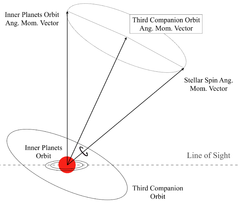
The radial velocity data show a long-term drift due to a third companion in the Kepler-56 system. Based on the linear trend of $0.8$ m s^-1 d^-1 determined from the simultaneous fit of the Kepler and radial-velocity data (§5), a third body in a circular orbit with a period $P_{\rm d}$ would have a minimum mass of $1.6M_{\rm J}(P_{\rm d}/\rm{yr})^{4/3}$. Hence, if the long-term velocity drift is seen to halt and reverse direction within the next few years, the third body would be implicated as another planet. The orbit of this more massive, outer companion dominates the angular momentum of the system, and hence can have a strong influence on the spin-orbit angle of the inner planets. If the third body is inclined by an angle $I_{3}$ relative to the mean orbital plane of the transiting planets, it would produce a torque on the planes of the inner planets and cause them to precess cyclically around the total angular momentum with a maximum inclination of $2I_{3}$. The planets in turn also cause the star to precess around the total angular momentum. However, the star precesses on a much slower timescale, resulting in large inclinations between the spin-axis of the host star and the orbital plane of the inner planets. The mutual inclination of the inner planets, on the other hand, remains low due to their compact orbits  (?). Figure S23 shows a graphical representation of this dynamical tilting hypothesis.

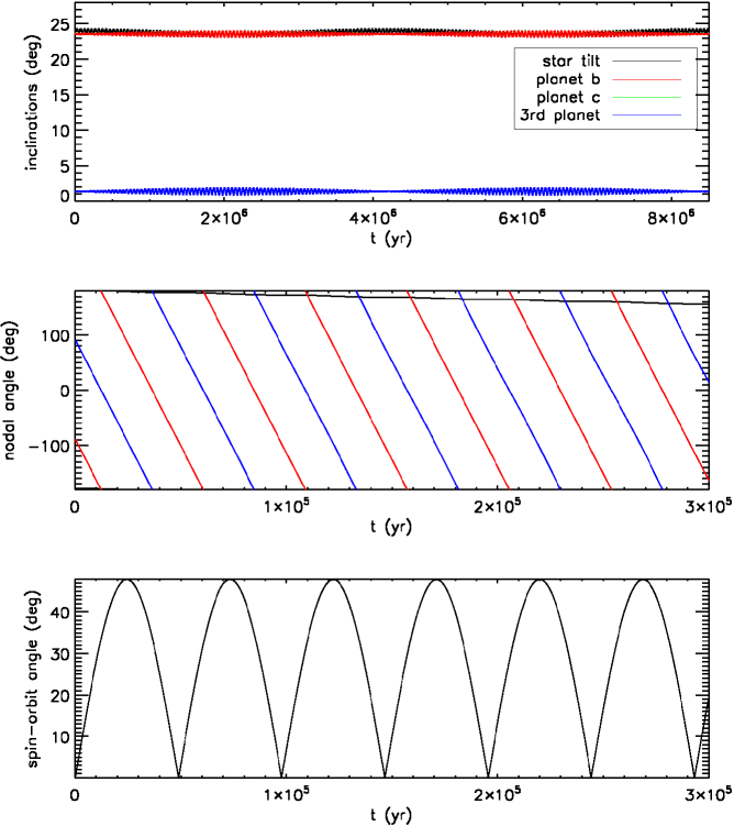
To quantify this scenario, we used the direct 3-planet code of Mardling & Lin  (?) to integrate the motion of such a system explicitly. These equations track the orbital trajectories of three planets, as well as the spin rate and direction of the star and the innermost planet. For concreteness we adopted the current star’s parameters, and assumed the outer body has a mass of 3.3 $M_{\rm J}$ planet with a semi-major axis of 2 AU, and eccentricity of 0.4. We furthermore assume a mutual inclination of $25^{\circ}$ of the outer planet with respect to the inner planet, the middle planet, and the stellar equatorial plane, all of which are initially aligned with one another. This choice for the inclination of the third body corresponds to a typical value for planets on wide orbits produced by planet-planet scattering  (?, ?). Table S6 gives the initial conditions of the simulation. Figure S24 shows the evolution of the inclinations of all relevant angles of the system over a timescale of $3\times 10^{5}$ years. As suggested by the qualitative discussion above, the spin-orbit angle between the host star and the inner, transiting system can reach large angles due to the outer planet on an inclined, eccentric orbit, consistent with our observations in the Kepler-56 system.

This simulation provides a proof of concept for the scenario described in the main text. We emphasize, though, that the properties of the companion were chosen somewhat arbitrarily. Furthermore, for this calculation we adopted the properties for the host star in its current evolutionary stage, but it should be borne in mind that the dynamical action may have occurred long ago when the star was on the main sequence or even the pre-main-sequence. Dynamical simulations including the evolution of the host star would allow study the effects of mass loss or tides on the planets  (?), and potentially constrain when the instability occurred. However, for a smaller host star, the precession of the star would occur with an even longer period, and hence produce a smaller torque on the inner planets than it currently does. Hence there would be even less difficulty producing a large spin-orbit misalignment.

Host Star
Mass ($M_{\odot}$)	1.32
Radius ($R_{\odot}$)	4.23
Apsidal motion constant	0.004
Moment of inertia coefficent	0.02
Obliquity (deg)	0.0
Planet b
Eccentricity	0.0
Semi-major axis (AU)	0.1028
Inclination relative to third companion (deg)	25.0
Argument of perigee (deg)	0.0
Longitude of line of nodes (deg)	0.0
True anomaly (deg)	57.0
Mass ($M_{\rm J}$)	0.069
Radius ($R_{\rm J}$)	0.3
Apsidal motion constant	0.15
Moment of inertia coefficient	0.25
Planet c
Eccentricity	0.0
Semi-major axis (AU)	0.1652
Inclination relative to third companion (deg)	25.0
Argument of perigee (deg)	0.0
Longitude of line of nodes (deg)	0.0
True anomaly (deg)	182.0
Mass ($M_{\rm J}$)	0.569
Third Companion
Eccentricity	0.4
Semi-major axis (AU)	2.0
True anomaly (deg)	256.0
Mass ($M_{\rm J}$)	3.3

Table S6: Initial conditions of the dynamical simulation of the Kepler-56 system, including a third companion on an eccentric and inclined orbit.

Figure S23: Graphical illustration of the dynamical tilting hypothesis for the Kepler-56 system. Note that the sizes are not to scale.

Figure S24: Simulation results demonstrating the generation of spin-orbit misalignment from the torque from a wide-orbiting, inclined companion. Initially, the observed system of two transiting planets is placed on coplanar orbits in the equatorial plane of their host star. A massive, inclined, and eccentric planet is placed exterior to them. Panel (a): Inclinations with respect to the Laplace plane (the plane normal to the total angular momentum), each of which stay nearly constant. Panel (b): Nodal angles versus simulation time. The inner and middle planets precess in concert, with the same nodal angle. The outer planet precesses at the same rate, but $180^{\circ}$ out of phase. The star precesses very slowly, due to its weak coupling to the planets. Panel (c): Angle between the stellar equator plane and the inner planet’s orbital plane. Both planets and the star remain $24^{\circ}$ inclined from the Laplace plane, but they precess at different rates, and hence are periodically misaligned by $48^{\circ}$.

References and Notes

- 1. W. J. Borucki, et al., Science 327, 977 (2010).
- 2. N. M. Batalha, et al., ApJ 713, L109 (2010).
- 3. W. J. Borucki, et al., ApJ 736, 19 (2011).
- 4. J. H. Steffen, et al., MNRAS 428, 1077 (2013).
- 5. J. De Ridder, et al., Nature 459, 398 (2009).
- 6. Materials, methods are available as supporting material on Science Online. .
- 7. W. A. Dziembowski, D. O. Gough, G. Houdek, R. Sienkiewicz, MNRAS 328, 601 (2001).
- 8. J. Montalbán, A. Miglio, A. Noels, R. Scuflaire, P. Ventura, ApJ 721, L182 (2010).
- 9. P. G. Beck, et al., Science 332, 205 (2011).
- 10. T. R. Bedding, et al., Nature 471, 608 (2011).
- 11. L. Gizon, S. K. Solanki, ApJ 589, 1009 (2003).
- 12. P. G. Beck, et al., Nature 481, 55 (2012).
- 13. D. Fabrycky, S. Tremaine, ApJ 669, 1298 (2007).
- 14. M. Nagasawa, S. Ida, T. Bessho, ApJ 678, 498 (2008).
- 15. D. Lai, F. Foucart, D. N. C. Lin, MNRAS 412, 2790 (2011).
- 16. T. M. Rogers, D. N. C. Lin, H. H. B. Lau, ApJ 758, L6 (2012).
- 17. M. R. Bate, G. Lodato, J. E. Pringle, MNRAS 401, 1505 (2010).
- 18. R. A. Mardling, MNRAS 407, 1048 (2010).
- 19. K. Batygin, Nature 491, 418 (2012).
- 20. D. Queloz, et al., A&A 359, L13 (2000).
- 21. J. N. Winn, et al., ApJ 631, 1215 (2005).
- 22. J. A. Johnson, et al., PASP 121, 1104 (2009).
- 23. J. N. Winn, D. Fabrycky, S. Albrecht, J. A. Johnson, ApJ 718, L145 (2010).
- 24. A. H. M. J. Triaud, et al., A&A 524, A25 (2010).
- 25. S. Albrecht, et al., ApJ 757, 18 (2012).
- 26. D. N. C. Lin, P. Bodenheimer, D. C. Richardson, Nature 380, 606 (1996).
- 27. J.-B. Le Bouquin, et al., A&A 498, L41 (2009).
- 28. C. A. Watson, et al., MNRAS 413, L71 (2011).
- 29. T. Hirano, et al., ApJ 759, L36 (2012).
- 30. R. Sanchis-Ojeda, et al., Nature 487, 449 (2012).
- 31. W. J. Chaplin, et al., ApJ 766, 101 (2013).
- 32. J. M. Jenkins, et al., ApJ 713, L120 (2010).
- 33. A. Savitzky, M. J. E. Golay, Analytical Chemistry 36, 1627 (1964).
- 34. N. M. Batalha, et al., ApJS 204, 24 (2013).
- 35. D. Huber, et al., Communications in Asteroseismology 160, 74 (2009).
- 36. S. Hekker, et al., MNRAS 402, 2049 (2010).
- 37. S. Hekker, et al., A&A 525, A131 (2011).
- 38. G. A. Verner, et al., MNRAS 415, 3539 (2011).
- 39. S. Hekker, et al., A&A 520, A60 (2010).
- 40. R. Handberg, T. L. Campante, A&A 527, A56 (2011).
- 41. T. R. Bedding, H. Kjeldsen, Communications in Asteroseismology 161, 3 (2010).
- 42. T. R. Bedding, et al., ApJ 713, L176 (2010).
- 43. S. Deheuvels, et al., ApJ 756, 19 (2012).
- 44. B. Mosser, et al., A&A 548, A10 (2012).
- 45. L. Gizon, et al., Proceedings of the National Academy of Science 110, 13267 (2013).
- 46. T. Toutain, T. Appourchaux, A&A 289, 649 (1994).
- 47. O. Benomar, T. Appourchaux, F. Baudin, A&A 506, 15 (2009).
- 48. M. Gruberbauer, T. Kallinger, W. W. Weiss, D. B. Guenther, A&A 506, 1043 (2009).
- 49. G. Houdek, N. J. Balmforth, J. Christensen-Dalsgaard, D. O. Gough, A&A 351, 582 (1999).
- 50. G. Houdek, Proceedings of SOHO 18/GONG 2006/HELAS I, Beyond the spherical Sun, K. Fletcher & M. Thompson, ed. (Noordwijk: ESA, 2006), vol. 624 of ESA Special Publication.
- 51. W. J. Chaplin, G. Houdek, C. Karoff, Y. Elsworth, R. New, A&A 500, L21 (2009).
- 52. M.-A. Dupret, et al., A&A 506, 57 (2009).
- 53. D. Huber, et al., ApJ 723, 1607 (2010).
- 54. F. Baudin, et al., A&A 529, A84 (2011).
- 55. T. Appourchaux, et al., A&A 537, A134 (2012).
- 56. E. Corsaro, et al., ApJ 757, 190 (2012).
- 57. W. J. Chaplin, et al., MNRAS 287, 51 (1997).
- 58. D. C. Fabrycky, J. N. Winn, ApJ 696, 1230 (2009).
- 59. T. Hirano, et al., ApJ 756, 66 (2012).
- 60. M. C. Stumpe, et al., PASP 124, 985 (2012).
- 61. J. C. Smith, et al., PASP 124, 1000 (2012).
- 62. A. A. Djupvik, J. Andersen, Highlights of Spanish Astrophysics V, J. M. Diego, L. J. Goicoechea, J. I. González-Serrano, J. Gorgas, eds. (Berlin: Springer, 2010), pp. 211–218.
- 63. L. A. Buchhave, et al., Nature 486, 375 (2012).
- 64. G. Torres, et al., ApJ 757, 161 (2012).
- 65. R. K. Ulrich, ApJ 306, L37 (1986).
- 66. T. M. Brown, R. L. Gilliland, R. W. Noyes, L. W. Ramsey, ApJ 368, 599 (1991).
- 67. H. Kjeldsen, T. R. Bedding, A&A 293, 87 (1995).
- 68. T. Kallinger, et al., A&A 509, A77 (2010).
- 69. B. Mosser, et al., A&A 517, A22 (2010).
- 70. D. Stello, et al., ApJ 700, 1589 (2009).
- 71. N. Gai, S. Basu, W. J. Chaplin, Y. Elsworth, ApJ 730, 63 (2011).
- 72. D. Huber, et al., ApJ 767, 127 (2013).
- 73. A. Miglio, Red Giants as Probes of the Structure and Evolution of the Milky Way, A. Miglio, J. Montalbán, A. Noels, eds., ApSS Proceedings (Berlin: Springer, 2012).
- 74. D. Huber, et al., ApJ 760, 32 (2012).
- 75. V. Silva Aguirre, et al., ApJ 757, 99 (2012).
- 76. K. Belkacem, et al., A&A 530, A142 (2011).
- 77. K. Belkacem, SF2A-2012: Proceedings of the Annual meeting of the French Society of Astronomy and Astrophysics, S. Boissier, et al., eds. (2012), pp. 173–188.
- 78. A. Miglio, et al., European Physical Journal Web of Conferences (2013), vol. 43 of European Physical Journal Web of Conferences, pp. 3004, DOI: 10.1051/epjconf/20134303004.
- 79. L. da Silva, et al., A&A 458, 609 (2006).
- 80. S. Basu, et al., ApJ 729, L10 (2011).
- 81. A. Miglio, et al., MNRAS 429, 423 (2013).
- 82. V. Silva Aguirre, et al., ApJ 769, 141 (2013).
- 83. D. Huber, et al., ApJ 743, 143 (2011).
- 84. B. Mosser, et al., A&A 550, A126 (2013).
- 85. P. Ventura, F. D’Antona, I. Mazzitelli, Ap&SS 316, 93 (2008).
- 86. R. Scuflaire, et al., Ap&SS 316, 149 (2008).
- 87. H. Kjeldsen, et al., ApJ 682, 1370 (2008).
- 88. C. Aerts, J. Christensen-Dalsgaard, M. Cunha, D. W. Kurtz, Sol. Phys. 251, 3 (2008).
- 89. J. Christensen-Dalsgaard, Ap&SS 316, 13 (2008).
- 90. J. Christensen-Dalsgaard, Ap&SS 316, 113 (2008).
- 91. J. Christensen-Dalsgaard, et al., ApJ 713, L164 (2010).
- 92. T. R. White, et al., ApJ 743, 161 (2011).
- 93. J. Christensen-Dalsgaard, Sol. Phys. 220, 137 (2004).
- 94. A. Pietrinferni, S. Cassisi, M. Salaris, F. Castelli, ApJ 612, 168 (2004).
- 95. S. S. Vogt, et al., Society of Photo-Optical Instrumentation Engineers (SPIE) Conference Series, D. L. Crawford, E. R. Craine, eds. (1994), vol. 2198 of Society of Photo-Optical Instrumentation Engineers (SPIE) Conference Series, p. 362.
- 96. A. W. Howard, et al., ApJ 721, 1467 (2010).
- 97. G. W. Marcy, R. P. Butler, PASP 104, 270 (1992).
- 98. C. D. Murray, S. F. Dermott, Solar system dynamics (Princeton, NJ: Princeton Univ. Press, 1999).
- 99. R. A. Mardling, D. N. C. Lin, ApJ 573, 829 (2002).
- 100. W. H. Press, S. A. Teukolsky, W. T. Vetterling, B. P. Flannery, Numerical recipes in C++ : the art of scientific computing (Cambridge: Cambridge University Press, 2002).
- 101. K. Mandel, E. Agol, ApJ 580, L171 (2002).
- 102. D. Ragozzine, M. J. Holman, ArXiv e-prints (arXiv:1006.3727) (2010).
- 103. W. H. Press, Comments on Astrophysics 7, 103 (1978).
- 104. H. Kjeldsen, T. R. Bedding, A&A 529, L8 (2011).
- 105. S. Mathur, et al., ApJ 741, 119 (2011).
- 106. J. A. Carter, J. N. Winn, ApJ 704, 51 (2009).
- 107. C. ter Braak, J. Vrugt, Statistics and Computing 16, 239 (2006).
- 108. E. Agol, J. Steffen, R. Sari, W. Clarkson, MNRAS 359, 567 (2005).
- 109. Y. Lithwick, J. Xie, Y. Wu, ApJ 761, 122 (2012).
- 110. M. Gladman, Icarus 106 (1992).
- 111. C. Marchal, G. Bozis, Celestial Mechanics 26 (1982).
- 112. R. Bulirsch, R. Stoer, Introduction to Numerical Analysis (New York:Springer-Verlag, 1991).
- 113. J. Wisdom, M. Holman, AJ 102 (1991).
- 114. J. Wisdom, M. Holman, J. Touma, Fields Institute Communications 10, 217, URL: web.mit.edu/wisdom/www/Symplectic_Correctors.pdf (1996).
- 115. J. E. Chambers, F. Migliorini, BAAS 29 (1997).
- 116. A. Nobili, I. Roxburgh, Relativity in celestial mechanics and astrometry: High precision dynamical theories and observational verifications: Proceedings of the Symposium, Leningrad, USSR, May 28-31, 1985 (Dordrecht, D. Reidel Publishing Co., 1986), pp. 3105–110.
- 117. G. Takeda, R. Kita, F. A. Rasio, ApJ 683, 1063 (2008).
- 118. S. Chatterjee, E. B. Ford, S. Matsumura, F. A. Rasio, ApJ 686, 580 (2008).
- 119. G. Voyatzis, J. D. Hadjidemetriou, D. Veras, H. Varvoglis, MNRAS 430, 3383 (2013).