Hamiltonian quantum simulation with bounded-strength controls
Abstract
We propose dynamical control schemes for Hamiltonian simulation in many-body quantum systems that avoid instantaneous control operations and rely solely on realistic bounded-strength control Hamiltonians. Each simulation protocol consists of periodic repetitions of a basic control block, constructed as a suitable modification of an “Eulerian decoupling cycle,” that would otherwise implement a trivial (zero) target Hamiltonian. For an open quantum system coupled to an uncontrollable environment, our approach may be employed to engineer an effective evolution that simulates a target Hamiltonian on the system, while suppressing unwanted decoherence to the leading order. We present illustrative applications to both closed- and open-system simulation settings, with emphasis on simulation of non-local (two-body) Hamiltonians using only local (one-body) controls. In particular, we provide simulation schemes applicable to Heisenberg-coupled spin chains exposed to general linear decoherence, and show how to simulate Kitaev’s honeycomb lattice Hamiltonian starting from Ising-coupled qubits, as potentially relevant to the dynamical generation of a topologically protected quantum memory. Additional implications for quantum information processing are discussed.
pacs:
03.67.Lx, 03.65.Fd, 03.67.-amit-ctp 4504
1 Introduction
The ability to accurately engineer the Hamiltonian of complex quantum systems is both a fundamental control task and a prerequisite for quantum simulation, as originally envisioned by Feynman [1, 2, 3]. The basic idea underlying Hamiltonian simulation is to use an available quantum system, together with available (classical or quantum) control resources, to emulate the dynamical evolution that would have occurred under a different, desired Hamiltonian not directly accessible to implementation [4]. From a control-theory standpoint, the simplest setting is provided by open-loop Hamiltonian engineering in the time domain [5, 6], whereby coherent control over the system of interest is achieved solely based on suitably designed time-dependent modulation (most commonly sequences of control pulses), without access to ancillary quantum resources and/or measurement and feedback. While open-loop Hamiltonian engineering techniques have their origin and a long tradition in nuclear magnetic resonance (NMR) [8, 7], the underlying physical principles of “coherent averaging” have recently found widespread use in the context of quantum information processing (QIP), leading in particular to dynamical symmetrization and dynamical decoupling (DD) schemes for control and decoherence suppression in open quantum systems [9, 10, 11, 12, 13, 14].
As applications for quantum simulators continue to emerge across a vast array of problems in physics and chemistry, and implementations become closer to experimental reality [3, 15, 16], it becomes imperative to expand the repertoire of available Hamiltonian simulation procedures, while scrutinizing the validity of the relevant control assumptions. With a few exceptions (notably, the use of so-called “perturbation theory gadgets” [17]), open-loop Hamiltonian simulation schemes have largely relied thus far on the ability to implement sequences of effectively instantaneous, “bang-bang” (BB) control pulses [18, 19, 20, 21, 22, 23, 24, 25]. While this is a convenient and often reasonable first approximation, instantaneous pulses necessarily involve unbounded control amplitude and/or power, something which is out of reach for many control devices of interest and is fundamentally unphysical. In the context of DD, a general approach for achieving (to at least the leading order) the same dynamical symmetrization as in the BB limit was proposed in [26], based on the idea of continuously applying bounded-strength control Hamiltonians according to an Eulerian cycle, so-called Eulerian DD (EDD). From a Hamiltonian engineering perspective, EDD protocols translate directly into bounded-strength simulation schemes for specific effective Hamiltonians – most commonly, the trivial (zero) Hamiltonian in the case of “non-selective averaging” for quantum memory (or “time-suspension” in NMR terminology). More recently, EDD has also served as the starting point for bounded-strength gate simulation schemes in the presence of decoherence, so-called dynamically corrected gates (DCGs) for universal quantum computation [27, 28, 29, 30].
In this work, we show that the approach of Eulerian control can be further systematically exploited to construct bounded-strength Hamiltonian simulation schemes for a broad class of target evolutions on both closed and open (finite-dimensional) quantum systems. Our techniques are device-independent and broadly applicable, thus substantially expanding the control toolbox for programming complex Hamiltonians into existing or near-term quantum simulators subject to realistic control assumptions.
The content is organized as follows. We begin in Sect. II by introducing the appropriate control-theoretic framework and by reviewing the basic principles underlying open-loop simulation via average Hamiltonian theory, along with its application to Hamiltonian simulation in the BB setting. Sect. III is devoted to constructing and analyzing simulation schemes that employ bounded-strength controls: while Sec. III.A reviews required background material on EDD, Sec. III.B introduces our new Eulerian simulation protocols for a generic closed quantum system. In Sec. III.C we separately address the important problem of Hamiltonian simulation in the presence of slowly-correlated (non-Markovian) decoherence, identifying conditions under which a desired Hamiltonian may be enacted on the target system while simultaneously decoupling the latter from its environment, and making further contact with DCG protocols. Sect. IV presents a number of illustrative applications of our general simulation schemes in interacting multi-qubit networks. In particular, we provide explicit protocols to simulate a large family of two-body Hamiltonians in Heisenberg-coupled spin systems additionally exposed to depolarization or dephasing, as well as to achieve Kitaev’s honeycomb lattice Hamiltonian starting from Ising-coupled qubits. In all cases, only local (single-qubit, possibly collective) control Hamiltonians with bounded strength are employed. A brief summary and outlook conclude in Sec. V.
2 Principles of Hamiltonian simulation
2.1 Control-theoretic framework
We consider a quantum system , with associated Hilbert space , whose evolution is described by a time-independent Hamiltonian . As mentioned, Hamiltonian simulation is the task of making evolve under some other time-independent target Hamiltonian, say, . Without loss of generality, both the input and the target Hamiltonians may be taken to be traceless. Two related scenarios are worth distinguishing for QIP purposes:
Closed-system simulation, in which case coincides with the quantum system of interest, (also referred to as the “target” henceforth), which undergoes purely unitary (coherent) dynamics;
Open-system simulation, in which case is a bipartite system on , where represents an uncontrollable environment (also referred to as bath henceforth), and the reduced dynamics of the target system is non-unitary in general.
In both cases, we shall assume the target system to be a network of interacting qudits, hence , for finite and . In the general open-system scenario, the joint Hamiltonian on may be expressed in the following form,
| (1) |
where the operators ( and () act on () respectively, and all the bath operators are assumed to be norm-bounded, but otherwise unspecified (potentially unknown). The closed-system setting is recovered from Eq. (1) in the limit . Likewise, we may express the target Hamiltonian in a similar form, with two simulation tasks being of special relevance: , in which case the objective is to realize a desired system Hamiltonian while dynamically decoupling from its bath , thereby suppressing unwanted decoherence [11]; or, more generally, and , where the simulated, dynamically symmetrized error generators may allow for decoherence-free subspaces or subsystems to exist [13, 31].
Formally, the dynamics is modified by an open-loop controller acting on the target system according to
| (2) |
where the operators and the (real) functions represent the available control Hamiltonians and the corresponding, generally time-dependent, control inputs respectively. Clearly, if the Hamiltonian is contained in the admissible control set, the corresponding control problem is trivial and the desired time-evolution,
can be exactly simulated continuously in time. However, this level of control need not be available in settings of interest, including open quantum systems where control actions are necessarily restricted to the target system alone, in Eq. (2). Following the general idea of “analog” quantum simulation [3], we shall assume in what follows a restricted set of control Hamiltonians (in a sense to be made more precise later) and focus on the task of approximately simulating the desired time evolution at a final time , or more generally, stroboscopically in time, that is, at instants , where
and is a fixed minimum time interval. Choosing sufficiently small allows in principle any desired accuracy in the approximation to be met, with the limit formally recovering the continuous limit.
Specifically, let and denote the unitary propagators associated to the total and the control Hamiltonians in Eq. (2), respectively:
| (3) | |||||
| (4) |
where we have set and indicates time-ordering, as usual. Then, for a given pair , we shall provide sufficient conditions for to be “reachable” from and, if so, devise a cyclic control procedure such that the resulting controlled propagator
| (5) |
where is the cycle time of the controller, that is, . In general, we shall allow for to differ from , corresponding to an overall scale factor in the simulated time, as it will become apparent later. If, for a fixed input Hamiltonian , arbitrary target Hamiltonians are reachable for given control resources, the simulation scheme is referred to as universal. In this case, complete controllability must be ensured by the tunable Hamiltonians in conjunction with the “drift” [6]. In contrast, we shall be especially interested in situations where control over is more limited.
Similar to DD protocols, Hamiltonian simulation protocols are most easily constructed and analyzed by effecting a transformation to the “toggling” frame associated to in Eq. (4) [7, 11, 14]. That is, evolution in the toggling frame is generated by the time-dependent, control-modulated Hamiltonian
| (6) |
with the corresponding toggling-frame propagator being related to the physical propagator in Eq. (3) by . Since the control propagator is cyclic and is time-independent, it follows that and, furthermore, acquires the periodicity of the controller, . Thus, the stroboscopic controlled dynamics of the system is determined by
| (7) |
Average Hamiltonian theory [7, 35] may then be invoked to associate an effective time-independent Hamiltonian to the evolution in the toggling-frame:
| (8) |
where is determined by the Magnus expansion [32], Explicitly, the leading-order term, determining evolution over a cycle up to the first order in time, is given by
| (9) |
with (absolute) convergence being ensured as long as [34]. Subject to convergence condition, higher-order corrections for evolution over time can also be upper-bounded by (see Lemma 4 in [33])
| (10) |
Ideally, one would like to achieve , so that equality would hold in Eq. (5) for all . In what follow, we shall primarily focus on achieving first-order simulation instead, by engineering the control propagator in such a way that
| (11) |
whereby, using Eq. (10) with ,
| (12) |
In general, the accuracy of the approximation in Eq. (11) improves as the “fast control limit”, , is approached. Physically, this corresponds to requiring that the shortest control time scale (pulse separation) involved in the control sequence be sufficiently small relative to the shortest correlation time of the dynamics induced by [35, 36]. While the problem of constructing general high-order Hamiltonian simulation schemes is of separate interest, we stress that second-order simulation can be readily achieved, in principle, by ensuring that is time-symmetric, namely, for . Since all odd-order Magnus corrections vanish in this case [35], it follows (by using again Eq. (10), with ), that , correspondingly boosting the accuracy of the simulation.
2.2 Hamiltonian simulation with bang-bang controls
BB Hamiltonian simulation provides the simplest control setting for achieving the intended objective, given in Eq. (5). Two main assumptions are involved: (i) First, we must be able to express the target Hamiltonian as
| (13) |
where are unitary operators on and the non-negative real numbers (not all zero). (ii) Second, the available control resources include a discrete set of instantaneous pulses on , whose application results in a piecewise-constant control propagator over , with corresponding toggling-frame propagators , , [9, 14]. Assumptions (i)-(ii) together allow for the time-average in Eq. (9) to be mapped to a convex (positive-weighted) sum. Eq. (13) may be interpreted as a sufficient condition for the target Hamiltonian to be reachable from given open-loop unitary control on alone. Reachable Hamiltonians must thus be at least as “disordered” as the input one in the sense of majorization [21, 14].
Specifically, Eq. (13) leads naturally to the following BB simulation scheme. Given simulation weights , define the following simulation intervals and timing pattern:
| (14) |
A piecewise-constant control propagator for the basic simulation block to be repeated may then be constructed as follows:
| (15) |
By using Eq. (9), it is immediate to verify that
| (16) |
resulting in the desired controlled evolution, Eqs. (11)-(12), provided that the convergence conditions for first-order simulation under are obeyed. Since, in practice, technological limitations always constrain the cycle duration to a finite minimum value , such conditions ultimately determine the maximum simulated time up to which evolution under may be reliably simulated using the physical Hamiltonian .
In analogy with BB DD schemes, realizing the prescription of Eq. (15) requires to discontinuously change the control propagator from to , via an instantaneous BB pulse at the th endpoint . As a result, despite its conceptual simplicity, BB simulation is unrealistic whenever large control amplitudes are not an option, and the evolution induced by during the application of a control pulse must be considered from the outset. This demands redesigning the basic control block in such a way that the actions of and are simultaneously accounted for.
3 Hamiltonian simulation with bounded controls
3.1 Eulerian simulation of the trivial Hamiltonian
The key to overcome the disadvantages of BB Hamiltonian simulation is to ensure that the control propagator varies smoothly (continuously) in time during each control cycle. We achieve this goal by relying on Eulerian control design [26]. To introduce the necessary group-theoretical background, we begin by revisiting how, for the special case of a target identity evolution (that is, , also corresponding to a “noop” gate, in terms of the end-time simulated propagator), EDD can be naturally interpreted as a bounded-strength simulation scheme.
In the Eulerian approach, the available control resources include a discrete set of unitary operations on , say, , , which are realized over a finite time interval through application of bounded-strength control Hamiltonians , with . That is,
| (17) |
Note that the choice of the control Hamiltonians is not unique, which allows for implementation flexibility. The unitaries are identified with the image of a generating set of a finite group under a faithful, unitary, projective representation [26]. That is, let be a finite group of order , such that each element may be written as an ordered product of elements in a generating set of order , be the representation map [37], and . The Cayley graph of relative to can be thought of as pictorially representing all elements of as strings of generators in . Each vertex represents a group element and a vertex is connected to another vertex by a directed edge “colored” (labeled) with generator if and only if . The number of edges in is thus equal to . Because a Cayley graph is regular, it always has an Eulerian cycle that visits each edge exactly once and starts (and ends) on the same vertex [38, 39]. Let us denote with the ordered list of generators defining an Eulerian cycle on which, without loss of generality, starts (and ends) at the identity element of .
Once a control Hamiltonian for implementing each generator as in Eq. (17) is chosen, an EDD protocol is constructed by assigning a cycle time as and by applying the control Hamiltonians sequentially in time, following the order determined by the Eulerian cycle . Thus,
| (18) |
where is the image of the generator labeling the th edge in . As established in [26], the lowest-order average Hamiltonian associated to the above EDD cycle has the form , where for any operator acting on , the map
| (19) |
projects onto the centralizer of (i.e., commutes with all ), and
| (20) |
implements an average of over both the control interval and the group generators. Accordingly, bounded-strength simulation of is achieved provided that the following DD condition is obeyed:
| (21) |
By Schur’s lemma, this is automatically ensured if the group representation acts irreducibly on . Formally, the BB limit may be recovered by letting for all [26], reflecting the ability to directly implement all the group elements (with no overhead, as if ) and corresponding to uniform simulation weights .
3.2 Eulerian simulation protocols beyond noop: Construction
We show how the Eulerian cycle method can be extended to bounded-strength simulation of a non-trivial class of target Hamiltonians. We assume that may be expressed as a convex unitary mixture of the group representatives ,
| (22) |
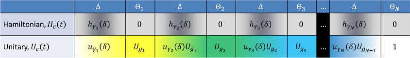
We construct the desired control protocol starting from an Eulerian cycle on . Specifically, the idea is to append to each of the control slots that define an EDD scheme a free-evolution (or “coasting”) period of suitable duration, in such a way that the net simulated Hamiltonian is modified from to as given in Eq. (22). A pictorial representation of the basic control block is given in Fig. 1. As in Eq. (17), let denote the minimum time duration required to implement each generator, hence, to smoothly change the control propagator from a value to along the cycle. While such “ramping up” control intervals have all the same length, each “coasting” interval is designed to keep the control propagator constant at for a duration determined by the corresponding weight . Since the control is switched off during coasting, continuity of the overall control Hamiltonian may be ensured, if desired, by requiring that
| (23) |
in addition to the bounded-strength constraint.
An Eulerian simulation protocol may be formally specified as follows. As before, let the th time interval be denoted as , , with and defining the cycle time . For each , let as in the BB case. The duration of the th coasting period is then assigned as
| (24) |
resulting in the following timing pattern [compare to Eq. (14)]:
| (25) |
As the expression for the cycle times makes it clear, the resulting protocol may be equivalently interpreted in two ways: starting from an EDD cycle, corresponding to and , we introduce the coasting periods to allow for non-trivial simulated dynamics to emerge; or, starting from a BB simulation scheme for , corresponding to , we introduce the ramping-up periods to allow for control Hamiltonians to be smoothly switched over . Either way, bounded-strength protocols imply a time-overhead relative to the BB case, recovering the BB limit as as expected. Explicitly, the control propagator for Eulerian simulation has the form:
| (26) | |||||
| (27) |
The resulting first-order Hamiltonian under Eulerian simulation is derived by evaluating the time-average in Eq. (9) with the control propagator given by Eqs. (26)-(27). Direct calculation along the lines of [26] yields:
where the last equality follows from two basic properties of Eulerian cycles: firstly, the list (and also ) of the vertices that are being visited contains each element precisely times; secondly, in traversing the Cayley graph, each group element is left exactly once by a -labeled edge for each generator . Thus, by recalling the definitions given in Eqs. (19) and (20), we finally obtain
| (28) |
which indeed achieves the intended first-order simulation goal, Eqs. (11)-(12), as long as convergence holds and the DD condition of Eq. (21) is obeyed.
The simulation accuracy may be improved by symmetrizing in time. In analogy to symmetrized EDD protocols [9], this can be easily accomplished by running the protocol and then suitably running it again in reverse. Specifically, let the duration of the coasting interval be changed as . Run the protocol as described above until time . Then, from time until time , modify Eqs. (26)-(27) as follows:
for . Provided that one is able to implement , we again obtain
while satisfying for , hence ensuring that .
3.3 Eulerian simulation while decoupling from an environment
The ability to implement a desired Hamiltonian on the target system , while switching off (at least to the leading order) the coupling to an uncontrollable environment , is highly relevant to realistic applications. That is, with reference to Eq. (1), the objective is now to simultaneously achieve , by unitary control operations acting on alone. Because the first-order Magnus term is additive [recall Eq. (9)], it is appropriate to treat each summand of individually, leading to a relevant average Hamiltonian of the form
where for a generic operator on we let
We can then apply the analysis of Sec. 3.2 to the internal system Hamiltonian () and each error generator () separately, to obtain in both cases a simulated operator of the form given in Eq. (28):
Since the task is to decouple from while maintaining the non-trivial evolution due to , the reachability condition of Eq. (22) must now ensure that
| (29) | |||||
| (30) |
Accordingly, it is necessary to extend the DD assumption of Eq. (21) to become
| (31) | |||||
| (32) |
such that holds for each of the summands in . Altogether we recover
It is interesting in this context to highlight some similarities and differences with DCGs [27], which also use Eulerian control as their starting point and are specifically designed to achieve a desired unitary evolution on the target system while simultaneously removing decoherence to the leading [27, 28, 30] or, in principle, arbitrarily high order [29]. By construction, the open-system simulation procedure just described does provide a first-order DCG implementation for the target gate : in particular, the requirement that Eqs. (29)-(30) be obeyed together (for the same weights ) is effectively equivalent to evading the “no-go theorem” for black-box DCG constructions established in [28], with the coasting intervals and the resulting “augmented” Cayley graph playing a role similar in spirit to a (first-order) “balance-pair” implementation. Despite these formal similarities, a number of differences exist between the two approaches: first, an obvious yet important difference is that DCG constructions focus directly on synthesizing a desired unitary propagator, as opposed to a desired Hamiltonian generator. Second, while the internal system Hamiltonian, , is a crucial input in a Hamiltonian simulation problem, it is effectively treated as an unwanted error contribution in analytical DCG constructions, in which case complete controllability over the target system must be supplied by the controls alone. Although in more general (optimal-control inspired) DCG constructions [30], limited external control is assumed and may become essential for universality to be maintained, emphasis remains, as noted above, on end-time synthesis of a target propagator. Finally, a main intended application of DCGs is realizing low-error single- and two-qubit gates for use within fault-tolerant quantum computing architectures, as opposed to robust Hamiltonian engineering for many-body quantum simulators which is our focus here.
3.4 Eulerian simulation protocols: Requirements
Before presenting explicit illustrative applications, we summarize and critically assess the various requirements that should be obeyed for Eulerian simulation to achieve the intended control objective of Eq. (5) in a closed or, respectively, open-system setting:
-
1.
Time independence. Both the internal Hamiltonian and the target Hamiltonian are taken to be time-independent (and, without loss of generality, traceless).
-
2.
Reachability. The target Hamiltonian must be reachable from , that is, there must be a control group , with a faithful, unitary projective representation mapping , such that Eq. (22) holds. For dynamically-corrected Eulerian simulation in the presence of an environment, this requires, as noted, that for the same weights , the desired system Hamiltonian is reachable from while the trivial (zero) Hamiltonian is reachable from each error generator separately, such that both Eqs. (29)-(30) hold together.
-
3.
Bounded control. For each generator of the chosen control group , we need access to bounded control Hamiltonians , such that application of over a time interval of duration realizes the group representative , additionally subject (if desired) to the continuity condition of Eq. (23).
- 4.
-
5.
Time-efficiency. If the choice of is not unique for given , the smallest group should be chosen, in order to keep the number of intervals per cycle, , to a minimum. In particular, efficient Hamiltonian simulation requires that (hence also ) scales (at most) polynomially with the number of subsystems .
The key simplification that the time-independence Assumption (1) introduces into the problem is that the periodicity of the control action is directly transferred to the toggling-frame Hamiltonian of Eq. (6), allowing one to simply focus on single-cycle evolution. Although this assumption is strictly not fundamental, general time-dependent Hamiltonians may need to be dealt with on a case-by-case basis (see also [40, 41, 42]). A situation of special practical relevance arises in this context for open systems exposed to classical noise, in which case and the system-bath interaction in Eq. (1) is effectively replaced by a classical, time-dependent stochastic field. Similar to DD and DCG schemes, Eulerian simulation protocols remain applicable as long as the noise process is stationary and exhibiting correlations over sufficiently long time scales [9, 43].
The reachability Assumption (2) is a prerequisite for Eulerian Hamiltonian simulation schemes. Although BB Hamiltonian simulation need not be group-based, most BB schemes follow this design principle alike. Assumption (3), restricting the admissible control resources to physical Hamiltonians with bounded amplitude (thus finite control durations, as opposed to instantaneous implementation of arbitrary group unitaries as in the BB case) is a basic assumption of the Eulerian control approach. As remarked, our premise is that the available Hamiltonian control is limited, restricted to only the target system if the latter is coupled to an environment, and typically non-universal on ; in particular, we cannot directly express and apply , or else the problem would be trivial. In addition to error-corrected Hamiltonian simulation in open quantum systems, scenarios of great practical interest may arise when the control Hamiltonians are subject to more restrictive locality constraints than the system and target Hamiltonians are (e.g., two-body simulation with only local controls, see also Sec. 4.1).
The required decoupling conditions in Assumption (4) are automatically obeyed if the representation acts irreducibly on . This follows directly from Schur’s lemma, together with the fact that the map defined in Eq. (20) is trace-preserving, and both and can be taken to be traceless. While convenient, irreducibility is not, however, a requirement. When the representation is reducible, care must be taken in order to ensure that Assumption (4) is nevertheless obeyed. It should be stressed that this is possible independently of the target Hamiltonian . Therefore, if the choice () works for one Eulerian simulation scheme (whether is irreducible or not), then it can be used for Eulerian simulation with any target that belongs to the reachable set from , that is, that can satisfy Eq. (22).
We close this discussion by recalling that it is always possible for a finite-dimensional target system to find a control group for which both Assumptions (2) and (4) are satisfied, by resorting to the concept of a transformer [22, 14]. A transformer is a pair , where is a finite group and is a faithful, unitary, projective representation such that, for any traceless Hermitian operators and on with , one may express
We illustrate this general idea in the simplest case of a single qubit, . Let denote the Pauli matrices and the unitary matrix defined by
| (33) |
which corresponds to a rotation by an angle about an axis . Direct calculation shows that and that conjugation by cyclically shifts the Pauli-matrices, i.e., , and . Consider now the group given by the presentation
Using the defining relations of this group, its elements can always be written as , where and . Clearly, the assignment given by yields a faithful, unitary, irreducible representation since the Pauli matrices commute up to phase. It is shown in [22] that the pair defines a transformer in the sense given above, namely, any traceless matrix may be reached from any fixed traceless, nonzero matrix , for suitable non-negative weights . The irreducibility property for any transformer pair can be easily established by contradiction [44].
A drawback of the transformer formalism is that general transformer groups tend to be large, making purely transformer-based simulation schemes inefficient. In practice, given the native system Hamiltonian , the challenge is to find a group that grants a reasonably efficient scheme while satisfying Assumptions (2) and (4), and subject to the ability to implement the required control operations. As we shall see next, transformer-inspired ideas may still prove useful in devising simulation schemes in the presence, for instance, of additional symmetry conditions.
4 Illustrative applications
In this section, we explicitly analyze simple yet paradigmatic Hamiltonian simulation tasks motivated by QIP applications. While a number of other interesting examples and generalizations may be envisioned (as also further discussed in the Conclusions), our goal here is to give a concrete sense of the usefulness and versatility of our Eulerian simulation approach in physically realistic control settings. In particular, we focus on achieving non-local Hamiltonian simulation using only bounded-strength local (single-qubit) control, in both closed and open multi-qubit systems.
4.1 Eulerian simulation in closed Heisenberg-coupled qubit networks
Let us start from the simplest case of a system consisting of qubits, interacting via an isotropic Heisenberg Hamiltonian of the form
where has units of energy and the second equality defines an equivalent compact notation. We are interested in a class of target XYZ Hamiltonians of the form
| (34) |
For instance, , corresponds to an isotropic XX model, whereas if with , an XXZ interaction is obtained, the special value corresponding to the important case of a dipolar Hamiltonian. The construction of a simulation protocol starts from observing that Hamiltonians as in Eq. (34) are reachable from , in the sense of Eq. (22), based on single-qubit control only.
Specifically, let , and let the representation map to . That is, is mapped to the following set of unitaries:
| (35) |
Choosing the generators of to be and , we assume that we have access to the control Hamiltonians
where the control inputs and satisfy and , for . Recalling Eq. (17), this yields the control propagators
with and (up to phase), as desired.
Note that for any single-qubit Hamiltonians and , averaging over the unitary group in Eq. (35) results in the following projection super-operator:
| (36) |
In general, the map is trace-preserving and, in this case, it acts non-trivially only on the first qubit. Thus, is trace-preserving on the first qubit. Since each term in is traceless in the first qubit, the decoupling condition follows directly from Eq. (36), even though the relevant representation is, manifestly, reducible.
Having satisfied our main requirements for Eulerian simulation, reachability of XYZ Hamiltonians as in Eq. (34) is equivalent to the existence of a solution to the following set of conditions:
| (37) | |||
for non-negative weights . While infinitely many choices exist in general, minimizing the total weight keeps the simulation time overhead to a minimum. For instance, it is easy to verify that a dipolar Hamiltonian of the form
may be simulated with minimum time overhead by choosing weights
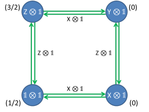
The Cayley graph associated with the resulting Eulerian simulation protocol is depicted in Fig. 2, with the explicit timing structure of the control block as in Fig. 1 and control segments per block. It is worth observing that although the weights and are zero in the particular case at hand, all group members of are nonetheless required, and the unitaries and still show up in the simulation scheme (during the ramping-up sub-intervals, as evident from Eq. (26)). This is crucial to guarantee that the unwanted term is projected out.
The above analysis and simulation protocols can be easily generalized to a chain of qubits (or spins), subject to nearest-neighbor (NN) homogeneous Heisenberg couplings, that is, a Hamiltonian of the form
where for later reference we have introduced the standard compact notation and we assume for concreteness that is even. In this case, we need only change the unitary representation of to be defined by the two generators and , resulting in the set of unitaries [42]
Physically, the required generators and correspond to control Hamiltonians that are still just sums of 1-local terms, and that act non-trivially on odd qubits only:
We expect that the design of Eulerian simulation schemes for more general scenarios where both the input and the target are arbitrary two-body Hamiltonians (including, for instance, long-range couplings) will greatly benefit from the existence of combinatorial approaches for constructing efficient DD groups [45, 41]. A more in-depth analysis of this topic is, however, beyond our current scope.
4.2 Error-corrected Eulerian simulation in open Heisenberg-coupled qubit networks
Imagine now that the Heisenberg-coupled system considered in the previous section is coupled to an environment , and the task is to achieve the desired XYZ Hamiltonian simulation while also removing arbitrary linear decoherence to the leading order. The total input Hamiltonian has the form
| (38) |
where and , for each and , are operators acting on , whose norm is sufficiently small to ensure convergence of the relevant Magnus series, similar to first-order DCG constructions [27, 28]. The target Hamiltonian then reads
in terms of suitable coupling-strength parameters as in Eq. (34). As before, we start by analyzing the case of qubits in full detail. Our strategy to synthesize a dynamically corrected simulation scheme involves two stages: (i) We will first decouple from , while leaving the system Hamiltonian unaffected; (ii) We will then apply the closed-system protocol of Sec. 4.1 to convert into the target system Hamiltonian . Once a suitable group and weights are identified in this way, both stages are carried out simultaneously in application.
A suitable DD group able to suppress general linear decoherence is provided by , under the -fold tensor power representation yielding (see also [28]):
generated, for instance, by the two collective generators and . In addition to the order of being minimal, with independently of , step (i) above is automatically satisfied for the input Hamiltonian at hand, since
| (39) |
Given a generic operator on , we may define the superoperator as
corresponding to weights given by
In step (ii), we still rely on the group , but now under a different representation. We choose the representation yielding the set of Eq. (35), with the same single-qubit generators , , and the corresponding weights determined by the solution of Eqs. (37). Define the superoperator to act as
Then the combined action of the two superoperators and yields
| (40) |
where , with unitary representation elements corresponding to the full Pauli group on two qubits:
The above representation is irreducible, with implementing the complete depolarizing channel on two qubits:
for every input . Together with the fact that all of the system terms in are traceless and is trace-preserving, this ensures that the DD conditions of Eqs. (31)-(32) are satisfied. Since and , the resulting Eulerian simulation cycle will involve in general time segments, with the number of non-zero weights (hence the total weight and the time-overhead of the simulation) being determined by the details of the error model and/or the target Hamiltonian.
A practically important case, where simpler simulation schemes are possible, occurs if qubits couple to their environment along a fixed axis, effectively corresponding to pure dephasing – say, for concreteness, that for in Eq. (38). A smaller DD group suffices in this case [28], namely , represented again in terms of collective qubit rotations,
and generated by the single element . Clearly, the commutation relationship in Eq. (39) is maintained, still allowing our two-step procedure to be followed. In this case, the combined group for simulation is , with , , reducibly represented as follows on the two-qubit space:
| (41) |
Suppose, for instance, that the task is to simulate a dipolar Hamiltonian as in Sec. 4.1. By following the above general procedure, with weights given by for alone, it is easy to see that Eq. (40) simplifies, leading to simulation weights with the remaining 4 weights equal to 0. While this implies that the simulation can now be achieved with only segments per cycle and minimum weight , care is needed in ensuring that the DD conditions in Eqs. (31)-(32), are still obeyed. This may be checked by inspection. In particular, the fact that for follows by analyzing the structure of each toggling-frame “error Hamiltonian”, , for , and verifying that no term proportional to is generated, that would be left uncorrected by averaging over the representation in Eq. (41). Likewise, the fact that for may be directly established by a similar calculation, or by using the trace argument in Sec. 4.1 for the two group generators and , while also noting that for the third generator , we have and the latter is decoupled by the representation in Eq. (41), . Thus, Eulerian Hamiltonian simulation in the presence of single-axis errors can be efficiently achieved.
Again, the schemes we have just presented for can be generalized to a chain consisting of spins, which interact according to a NN Heisenberg interaction and are each linearly coupled to the environment, according to Eq. (38). In this case, exploiting the results of Sec. 4.1, a useful group for simulation is provided by , under the unitary representation
corresponding to generators , all of which can be implemented using only 1-local (single-qubit) Hamiltonians. As before, each simulation cycle will consist in the general case of arbitrary linear decoherence of time segments. Despite the reducibility of the above representation (with the full Pauli group on qubits consisting of elements), the DD conditions given by Eqs. (31)-(32) remain valid for reasons similar to those outlined for under pure dephasing.
4.3 Eulerian simulation of Kitaev’s honeycomb lattice Hamiltonian
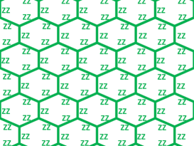
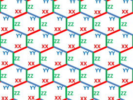
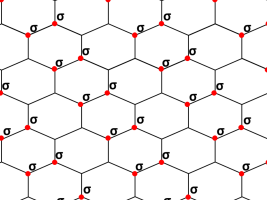
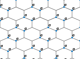
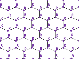
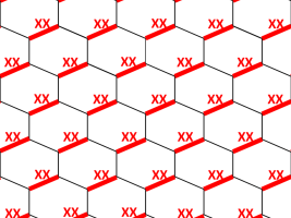
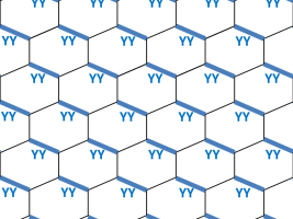
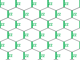
We return to Eulerian simulation in closed quantum systems, but tackle a more complicated Hamiltonian of paradigmatic relevance to topological quantum memories, namely, Kitaev’s honeycomb lattice model [46]. Suppose that the target system consists of a network of qubits arranged on a honeycomb lattice and interacting via NN Ising couplings. The relevant Hamiltonian is graphically displayed in Fig. 3(left), where vertices represent qubits and edges represent two-qubit couplings of the form , with vertices and being adjacent in the graph and indicating, as before, the Pauli operator acting non-trivially only on qubit . The target Hamiltonian is shown in Fig. 3(right), where some of the edges are now of the form and . In accordance with the figure, we shall also call the -edges forward-slashes, the -edges back-slashes, and the -edges verticals henceforth.
The basic idea to accomplish this simulation is to exploit the matrix given in Eq. (33), in conjunction with the symmetry of our problem: since all Hamiltonian terms are precisely two-local and of the homogeneous form , it will be possible to avoid using the full machinery of a transformer. Consider the group generated by the three unitaries, , and , where , shown in Fig. 4(left) with , has ’s on every second forward-slash, , shown in Fig. 4(center) with , has ’s on every second back-slash, and , shown in Fig. 4(right), has applied to every vertex. These unitaries can be generated by one-local Hamiltonians. By repeatedly conjugating and with , we immediately see that we can also perform and , shown in Fig. 4, for any . Note that up to phase, all such and commute. Because conjugation by maps Pauli matrices to Pauli matrices, for any Pauli we have , where is another Pauli matrix. Thus, up to phase, we can write any element of in the canonical form
| (42) |
where and only appears on the right.
To construct an Eulerian simulation protocol we must be able to choose so that is reachable from , i.e., obeys Eq. (22), while ensuring that the DD condition of Eq. (21) is also fulfilled. We start from the fact that
Observe that when , all forward-slash edges connect vertices that are acted upon by either or , while all other edges connect vertices that are operated by . Consequently, removes all Hamiltonian terms except for those along the forward-slashes; upon conjugating by , we may then convert these surviving terms to terms, as desired. To summarize,
gives the Hamiltonian shown in Fig. 5(left). Similarly, the effect of is to leave precisely the back-slash edges, which can be converted from to by conjugation by . Thus,
gives the Hamiltonian shown in Fig. 5(center). Lastly, it is not hard to see that the product has ’s on every second row of verticals; accordingly,
isolates precisely the verticals, giving the Hamiltonian shown in Fig. 5(right). In this case, no -conjugation is necessary since we wish to maintain edges along the verticals. Putting all these steps together, we conclude that
thus providing the desired weights for the Eulerian protocol. Since there are generators and, from Eq. (42), group elements, each control block consists of time intervals.
Lastly, we must verify that Eq. (21) holds. Note that acts via conjugating each vertex by unitaries (since the generating pulses are one-local), and since such an operation is trace-preserving at each vertex, this necessarily takes the precisely two-local terms in to precisely two-local terms in . Since no one-local terms can arise, all terms are of the form , where and are adjacent vertices and . Thus, we may write
Due to the canonical form of our group elements, Eq. (42), the action of reads
where and , respectively. Just as the map removes all non-forward-slash terms, the map depolarizes precisely one vertex of each pair of non-forward-slash vertices, and therefore suppresses all non-forward-slash terms. With only forward-slash terms remaining, , since the -sum removes all non-back-slash terms. Thus, we conclude that , as desired.
5 Conclusion and outlook
We have shown that the Eulerian cycle technique successfully employed in both dynamical decoupling schemes and dynamically corrected gates can be extended to also enable Hamiltonian quantum simulation with realistic bounded-strength controls. For given internal dynamics and control resources, we have characterized the family of reachable target Hamiltonians and provided constructive open-loop control protocols for stroboscopically implementing a desired evolution in the family with accuracy (at least) up to the second order in the sense of average Hamiltonian theory. We have additionally shown how Hamiltonian simulation may be accomplished in an open quantum system while simultaneously suppressing unwanted decoherence, provided that appropriate time-scale requirements and decoupling conditions are fulfilled. The usefulness and flexibility of our Eulerian simulation techniques have been explicitly illustrated through several QIP-motivated examples involving both unitary and open-system dynamics on interacting qubit networks. In all cases, access to purely local (single-qubit) control Hamiltonian is assumed, subject to finite-amplitude constraint.
It is our hope that our results may be of immediate relevance to ongoing efforts for developing and programming quantum simulators in the laboratory. A a number of possible generalizations and further theoretical questions may be worth considering. As an additional simulation problem dual to the one we analyzed for Heisenberg-coupled spin chains, exploring schemes where a target Heisenberg Hamiltonian is generated out of Ising couplings only would be of special interest, given the experimental availability of the latter in existing large-scale trapped-ion simulators [16]. Likewise, it could be useful to explore whether bounded-strength simulation as proposed here may be made compatible with open-loop filtering techniques for modulating coupling strengths, such as proposed in [47], as well as in [48] in conjunction with non-unitary control via field gradients. Building on existing results for dynamical decoupling schemes [42], the use and possible advantages of randomized simulation schemes in terms of efficiency and/or robustness may be yet another venue of investigation, especially in connection with large control groups. Lastly, it remains an important open question to determine whether simulation schemes able to guarantee a minimum fidelity over long evolution times may be devised, in the spirit of [49] for the particular case of the zero Hamiltonian.
Acknowledgements
L.V. is grateful to Guifrè Vidal for valuable discussions and early contributions to the subject of this work. This research was conducted while P.W. was visiting the Center for Theoretical Physics at MIT during a sabbatical leave from UCF. P.W. would like to thank Edward Farhi, Peter Shor, and their group members for their hospitality. This work was supported in part by the NSF Center for Science of Information, under grant No. CCF-0939370, as well as by the U.S. Department of Energy under cooperative research agreement contract No. DE-FG02-05ER41360. P.W. gratefully acknowledges support from NSF CAREER Award No. CCF-0746600. Work at Dartmouth was partially supported by the NSF under grant No. PHY-0903727, the U.S. Army Research Office under contract No. W911NF-11-1-0068, and the Constance and Walter Burke Special Project Fund in Quantum Information Science.
References
References
- [1] R. Feynman, Int. J. Theor. Phys. 21, 467 (1982).
- [2] S. Lloyd, Science 261, 1569 (1993).
- [3] I. Buluta and F. Nori, Science 326, 108 (2009); I. M. Georgescu, S. Ashhab, and F. Nori, arXiv:1308.6253.
- [4] This idea may be more generally applied to emulate a desired non-unitary (dissipative) evolution, see e.g. M. Müller, S. Diehl, G. Pupillo, and P. Zoller, arXiv:1203.6595, for a recent survey.
- [5] S. Schirmer, in: Lagrangian and Hamiltonian Methods for Nonlinear Control 2006, Lect. Notes in Control and Inf. Sciences 336, 293 (2007).
- [6] D. D’Alessandro, Introduction to Quantum Control and Dynamics (Chapman and Hall/CRC, Boca Raton, 2007).
- [7] R. R. Ernst, G. Bodenhausen, and A. Wokaun, Principles of Nuclear Magnetic Resonance in One and Two dimension (Clarendon Press, Oxford, 1987).
- [8] U. Haeberlen and J. S. Waugh, Phys. Rev. 175, 453 (1968).
- [9] D. A. Lidar and T. Brun (Editors), Quantum Error Correction (Cambridge University Press, 2013).
- [10] L. Viola and S. Lloyd, Phys. Rev. A 58, 2733 (1998).
- [11] L. Viola, E. Knill, and S. Lloyd, Phys. Rev. Lett. 82, 2417 (1999).
- [12] L. Viola, S. Lloyd, and E. Knill, Phys. Rev. Lett. 83, 4888 (1999).
- [13] P. Zanardi, Phys. Lett. A 258, 77 (1999).
- [14] L. Viola, Phys. Rev. A 66, 012307 (2002).
- [15] B. P. Lanyon, C. Hempel, D. Nigg, M. Müller, R. Gerritsma, F. Zähringer, P. Schindler, J. T. Barreiro, M. Rambach, G. Kirchmair, M. Hennrich, P. Zoller, R. Blatt, and C. F. Roos, Science 334, 57 (2011).
- [16] J. W. Britton, B. C. Sawyer, A. C. Keith, C.-C. J. Wang, J. K. Freericks, H. Uys, M. J. Biercuk, and J. J. Bollinger, Nature 484, 489 (2012).
- [17] S. Bravyi, D. P. DiVincenzo, D. Loss, and B. M. Terhal, Phys. Rev. Lett. 101, 070503 (2008).
- [18] P. Wocjan, D. Janzing, and T. Beth, Quantum Inf. Comput. 2, 117 (2002b).
- [19] J. L. Dodd, M. A. Nielsen, M. J. Bremner, and R. T. Thew, Phys. Rev. A 65, 040301 (2002).
- [20] P. Wocjan, M. Rötteler, D. Janzing, and T. Beth, Phys. Rev. A 65, 042309 (2002).
- [21] C. H. Bennett, J. I. Cirac, M. S. Leifer, D. W. Leung, N. Linden, S. Popescu, and G. Vidal, Phys. Rev. A 66, 012305 (2002).
- [22] P. Wocjan, M. Roetteler, D. Janzing, and T. Beth, Quantum Inf. Comput. 2, 133 (2002).
- [23] Y. C. Liu, Z. F. Xu, G. R. Jin, and L. You, Phys. Rev. Lett. 107, 013601 (2011).
- [24] T. Tanamoto, V. M. Stojanović, C. Bruder and D. Becker, Phys. Rev. A 87, 052305 (2013).
- [25] D. Becker, T. Tanamoto, A. Hutter, F. L. Pedrocchi, and D. Loss, arXiv:1302.3998.
- [26] L. Viola and E. Knill, Phys. Rev. Lett 90, 037901 (2002).
- [27] K. Khodjasteh and L. Viola, Phys. Rev. Lett. 102, 080501 (2009).
- [28] K. Khodjasteh and L. Viola, Phys. Rev. A 80, 032314 (2009).
- [29] K. Khodjasteh, D. A. Lidar, and L. Viola, Phys. Rev. Lett. 104, 090501 (2010).
- [30] K. Khodjasteh, H. Bluhm, and L. Viola, Phys. Rev. A 86, 042329 (2012).
- [31] L. Viola, E. Knill, and S. Lloyd, Phys. Rev. Lett. 85, 3520 (2000).
- [32] W. Magnus, Comm. Pure Appl. Math. 7, 649 (1954).
- [33] K. Khodjasteh and D. A. Lidar, Phys. Rev. A 78, 012355 (2008).
- [34] S. Blanes, F. Casas, J. A. Oteo, and J. Ros, Phys. Rep. 470, 151 (2009).
- [35] U. Haeberlen, High Resolution NMR in Solids: Selective Averaging, Adv. Magn. Res. 1 (Academic Press, 1976).
- [36] K. Khodjasteh, T. Erdélyi, and L. Viola, Phys. Rev. A 83, 023305(R) (2011).
- [37] Recall that a projective representation need only be a homomorphism up to phase, i.e., it obeys for , with proportionality rather than equality.
- [38] B. Bollobás, Modern Graph Theory, vol. 184 of Graduate Texts in Mathematics (Springer, 1998).
- [39] C. Godsil and G. Royle, Algebraic Graph Theory, vol. 207 of Graduate Texts in Mathematics (Springer, 2001).
- [40] L. Viola and E. Knill, Phys. Rev. Lett. 94, 060502 (2005).
- [41] L. F. Santos and L. Viola, Phys. Rev. Lett. 97, 150501 (2006).
- [42] L. F. Santos and L. Viola, New J. Phys. 10, 083009 (2008).
- [43] L. Cywinski, R. M. Lutchyn, C. P. Nave, and S. Das Sarma, Phys. Rev. B 77, 174509 (2008).
- [44] If were reducible, then there would exist a non-trivial invariant subspace such that . Hence, any Hamiltonian of the form , with being an orthonormal basis for , could only be transformed to other Hamiltonians of this same form, preventing from being a transformer.
- [45] M. Stollsteimer and G. Mahler, Phys. Rev. A 64, 052301 (2001).
- [46] A. Kitaev, Ann. Phys. 321, 2 (2006).
- [47] D. Hayes, S. T. Flammia, and M. J. Biercuk, arXiv:1309.6736.
- [48] A. Ashok and P. Cappellaro, Phys. Rev. Lett. 110, 220503 (2013).
- [49] K. Khodjasteh, J. Sastrawan, D. Hayes, T. J. Green, M. J. Biercuk, and L. Viola, Nature Commun. 4, 2045 (2013).