Applying compressed sensing to genome-wide association studies

Abstract

Background The aim of a genome-wide association study (GWAS) is to isolate DNA markers for variants affecting phenotypes of interest. Linear regression is employed for this purpose, and in recent years a signal-processing paradigm known as compressed sensing (CS) has coalesced around a particular class of regression techniques. CS is not a method in its own right, but rather a body of theory regarding signal recovery when the number of predictor variables (i.e., genotyped markers) exceeds the sample size. Results Using CS theory, we show that all markers with nonzero coefficients can be identified (selected) using an efficient algorithm, provided that they are sufficiently few in number (sparse) relative to sample size. For heritability $h^{2}=1$, there is a sharp phase transition from poor performance to complete selection as the sample size is increased. For heritability values less than one, complete selection can still occur, although the transition is smoothed. The transition boundary is only weakly dependent on the total number of genotyped markers. In the presence of correlations among predictor variables (linkage disequilibrium), measures of recovery such as the squared deviations of the estimated coefficients from their true values are also smoothed. More practical measures of signal recovery can accommodate linkage disequilibrium between a true causal variant and markers residing in the same genomic region, and indeed such measures (e.g., median $P$-value of selected markers) continue to show the good behavior expected in the absence of linkage disequilibrium. When applying this approach to the GWAS analysis of height, we show that 70-100% of the selected markers are strongly correlated with height-associated markers identified by the GIANT Consortium.

Conclusion The signal-processing paradigm known as CS is applicable to GWAS. The crossing of a transition boundary between distinct phases provides an objective means of determining when true trait-associated markers are being recovered, and we propose a novel analysis strategy that takes advantage of this property. The median $P$-value exhibits a sharp transition as the sample size is increased, indicating nearly complete recovery of true signal (causal variants or nearby proxy markers). In addition, given a limited sample size, it may still be possible to discover a phase transition by increasing the penalization, although in this case only a subset of the support can be recovered. Supposing that the recovery of the entire set is desired, we find for $h^{2}\sim 0.5$ that a sample size of approximately thirty times the number of markers with nonzero coefficients is sufficient.

Research

[id=n1]Correspondences to hsu@msu.edu or carsonc@mail.nih.gov

Background

The search for genetic variants associated with a given phenotype in a genome-wide association study (GWAS) is a classic example of what has been called a $p\gg n$ problem, where $n$ is the sample size (number of subjects) and $p$ is the number of predictor variables (genotyped markers) johnstone:2009 . Estimating the partial regression coefficients of the predictor variables by ordinary least squares (OLS) requires that the sample size exceed the number of coefficients, which in the GWAS context may be of order $10^{5}$ or even $10^{6}$. The difficulty of assembling such large samples has been one obstacle hindering the simultaneous estimation of all regression coefficients advocated by some authors hoggart:2008 ; goddard:2009:shrink ; kemper:2012:sheep .

The typical procedure in GWAS is to estimate each coefficient by OLS independently and retain those meeting a strict threshold; this approach is sometimes called marginal regression (MR) genovese:2012 . Although the implementation of MR in GWAS has led to an avalanche of discoveries visscher:2012:gwas , it is uncertain whether it will be optimal as datasets continue to increase in size. Many genetic markers associated with a trait are likely to be missed because they do not pass the chosen significance threshold yang:2010:snpherit .

Unlike MR, which directly estimates whether each coefficient is nonzero, an $L_{1}$-penalization algorithm such as the lasso effectively translates the estimates toward the origin, where many are truncated out of the model tibshirani:1996 . If the number of variants associated with a typical complex trait is indeed far fewer than the total number of polymorphic sites park:2011 ; stahl:2012 ; ripke:2013 , then it is reasonable to believe that $L_{1}$ penalization will at least be competitive with MR. Methods relying on the assumption of sparsity (few nonzero coefficients relative to sample size) have in fact been adopted by workers in the field of genomic selection (GS), which uses genetic information to guide the artificial selection of livestock and crops meuwissen:2001 ; deloscampos:2010 ; hayes:2010 ; meuwissen:2013 . Note that the aim of GS (phenotypic prediction) is somewhat distinct from that of GWAS (the identification of markers tagging causal variants). The lasso is one of the methods studied by GS investigators usai:2009 ; wimmer:2013 , although Bayesian methods that regularize the coefficients with strong priors tend to be favored zhou:2013:bslmm ; gianola:2013:gs .

In this paper we show that theoretical results from the field of compressed sensing (CS) supply a rigorous quantitative framework for the application of regularization methods to GWAS. In particular, CS theory provides a mathematical justification for the use of $L_{1}$-penalized regression to recover sparse vectors of coefficients and highlights the difference between selection of the markers with nonzero coefficients and the fitting of the precise coefficient values. CS theory also addresses the robustness of $L_{1}$ algorithms to the distribution of nonzero coefficient magnitudes.

Besides supplying a rule of thumb for the sample size sufficing to select the markers with true nonzero coefficients, CS gives an independent quantitative criterion for determining whether a given dataset has in fact attained that sample size. That is, whereas biological assumptions regarding the number of nonzeros do enter into the rule of thumb about sample size, these assumptions need not hold for the use of $L_{1}$ penalization to be justified; this is because the returned results themselves inform the investigator whether the assumptions are met.

We emphasize that CS is not a method per se but may be considered a general theory of regression that takes into account model complexity (sparsity). The theory is still valid in the classical regression domain of $n>p$ but establishes conditions for when full recovery of nonzero coefficients is still possible when $n<p$ donoho:2005 ; candes:2009 ; candes:2011:ripless . Our work therefore should not be directly compared to recent literature proposing and evaluating GS methods zhou:2013:bslmm ; gianola:2013:gs . Rather, our goal is to elucidate properties of well-known methods, already in use by GWAS and GS researchers, whose mathematical attributes and empirical prospects may be insufficiently appreciated.

Using more than 12,000 subjects from the ARIC European American and GENEVA cohorts and nearly 700,000 single-nucleotide polymorphisms (SNPs), we show that the matrix of genotypes acquired in GWAS obeys properties suitable for the application of CS theory. In particular, a given sample size determines the maximum number of nonzeros that will be fully selected using an $L_{1}$-penalization regression algorithm. If the sample size is too small, then the complete set of nonzeros will not be selected. The transition between poor and complete selection is sharp in the noiseless case (narrow-sense heritability equal to one). It is smoothed in the presence of noise (heritability less than one) but still fully detectable. Consistent with CS theory, we find in cases with realistic residual noise that the minimal sample size for full recovery is primarily determined by the number of nonzeros, depends very weakly on the number of genotyped markers candes:2006:rob ; donoho:2011 ; candes:2011:ripless , and is robust to the distribution of coefficient magnitudes donoho:2009 .

Theory of Compressed Sensing

The linear model of quantitative genetics is

$$\mathbf{y}=\mathbf{Ax}+\mathbf{e},$$ (1)

where $\mathbf{y}\in\mathbb{R}^{n}$ is the vector of phenotypes, $\mathbf{A}\in\mathbb{R}^{n\textrm{x}p}$ is the matrix of standardized genotypes, $\mathbf{x}\in\mathbb{R}^{p}$ is the vector of partial regression coefficients, and $\mathbf{e}\in\mathbb{R}^{n\textrm{x}1}$ is the vector of residuals. In the CS literature, $\mathbf{A}$ is often called the sensing or measurement matrix. Standardizing $\mathbf{A}$ does not affect the results and makes it simpler to utilize CS theory. We suppose that $\mathbf{x}$ contains $s$ nonzero coefficients (“nonzeros”) whose indices we wish to know.

The phase transition to complete selection is best quantified with two ratios $(\rho,\delta)$, where $\rho=s/n$ is a measure of the sparsity of nonzeros with respect to the sample size and $\delta=n/p$ is a measure of the undersampling. If we plot $\delta$ on the abscissa ($x$-axis) and $\rho$ on the ordinate ($y$-axis), we have a phase plane on the square $(0,1)\times(0,1)$, where each point represents a possible GWAS situation (sample size, number of genotyped markers, number of true nonzeros). The performance of any given method can be assessed by evaluating a measure of recovery quality at each point of the plane. For an arbitrary $p$-vector $\mathbf{x}$, we use the following notation for the $L_{1}$ and $L_{2}$ norms:

$$\|\mathbf{x}\|_{L_{1}}=\sum_{i=1}^{p}|x_{i}|\quad\textrm{and}\quad\|\mathbf{x}\|_{L_{2}}=\sqrt{\sum_{i=1}^{p}x_{i}^{2}}.$$

Our results rely on two lines of research in the field of CS, which we summarize as two propositions.

Proposition 1

donoho:2005 ; donoho:2006:neighbor ; donoho:2009:ptc_igor ; donoho:2011 Suppose that the entries of the sensing matrix $\mathbf{A}$ are drawn from independent normal distributions and $\mathbf{e}$ is the zero vector (noiseless case). Then the $\rho-\delta$ plane is partitioned by a curve $\rho=\rho_{L_{1}}(\delta)$ into two phases. Below the curve the solution of $\min\limits_{\hat{\mathbf{x}}}\|\hat{\mathbf{x}}\|_{L_{1}}$ subject to $\mathbf{A}\hat{\mathbf{x}}=\mathbf{y}$ leads to $\hat{\mathbf{x}}=\mathbf{x}$ with probability converging to one as $n,p,s\to\infty$ in such a way that $\rho$ and $\delta$ remain constant. Above the curve $\hat{\mathbf{x}}\neq\mathbf{x}$ with similarly high probability.

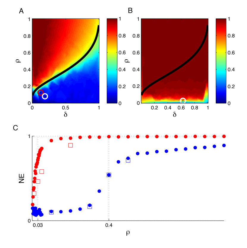
1 The function $\rho_{L_{1}}(\delta)$ can be analytically calculated donoho:2006:neighbor . Although Figure 1A presents some of our empirical results, which we will discuss below, it can be taken as an illustration of the meaning of Proposition 1. The color scale represents the goodness of recovery, and the black curve is the graph of $\rho_{L_{1}}(\delta)$. It can be seen that increasing the sample size relative to $s$ (decreasing $\rho$) leads to a sharp transition from poor to good recovery for $\delta<<1$ (i.e. $n<<p$). In other words, despite the fact that solving for $\mathbf{x}$ in $\mathbf{Ax}=\mathbf{y}$ is strictly speaking underdetermined given $n<p$, minimizing $||\hat{\mathbf{x}}||_{L_{1}}$ subject to the system of equations still yields recovery of $\mathbf{x}$ with high probability if $n$ is sufficiently large relative to $s$.

Most phenotypes do not have a heritability of one and thus are not noiseless, but CS theory shows that selection is still possible in this situation. Before stating the relevant CS result, we need to define two quantities characterizing the genotype matrix $\mathbf{A}$.

Definition 1

candes:2011:ripless The matrix $\mathbf{A}$ satisfies isotropy if the expectation value of $\mathbf{A}^{\prime}\mathbf{A}$ is equal to the identity matrix.

1 In the context of GWAS, a matrix of gene counts is isotropic if all markers are in linkage equilibrium (LE).

Definition 2

candes:2011:ripless The coherence of the matrix $\mathbf{A}$ is the smallest number $\gamma$ such that, for each row $\mathbf{a}$ of the matrix,

$$\max_{1\leq t\leq p}|\mathbf{a}_{t}|^{2}\leq\gamma.$$

A matrix of genotypes is thus reasonably incoherent if the magnitudes of the matrix elements do not differ greatly from each other. In the GWAS context, $\mathbf{A}$ will be reasonably incoherent if all markers with very low minor allele frequency (MAF) are pruned, since $\mathbf{A}$ is standardized and the standard deviation scales with MAF.

We can now state

Proposition 2

candes:2011:ripless Suppose that the sensing matrix $\mathbf{A}$ is isotropic with coherence $\gamma$. If $n>C\,\gamma\,s\log p$ for a constant $C$ then the solution of the problem

$$\min_{\hat{\mathbf{x}}}\bigg{[}\|\mathbf{y}-\mathbf{A}\hat{\mathbf{x}}\|^{2}_{L_{2}}+\lambda\|\hat{\mathbf{x}}\|_{L_{1}}\bigg{]}$$

with a suitable choice of $\lambda$ obeys

$$\|\hat{\mathbf{x}}-\mathbf{x}\|^{2}_{L_{2}}\leq\frac{\sigma^{2}_{E}}{n}s\operatorname*{polylog}p,$$

where $\sigma^{2}_{E}$ is the variance of the residuals in $\mathbf{e}$.

1 Two features of Proposition 2 are worth noting. First, no strong restrictions on $\mathbf{x}$ are required. Second, the critical threshold value of $n$ depends linearly on $s$ but only (poly)logarithmically on $p$. For $n$ larger than the critical value, the deviations of the estimated coefficients from the true values will follow the expected OLS scaling of $1/\sqrt{n}$.

These results are more powerful than they might seem from the restrictive hypotheses required for brief formulations. For example, it has been shown that a curve similar to that in Proposition 1 also demarcates a phase transition in the case of $\mathbf{e}\neq\mathbf{0}$ — although, as might be expected from a comparison of Propositions 1 and 2, with large residual noise the transition is to a regime of gradual improvement with $n$ rather than to instantaneous recovery donoho:2006:break ; donoho:2011 . A remarkable feature of this gradual improvement, however, should be noted. Proposition 2 states that the scaling of the total fitting error in the favorable regime is within a (poly)logarithmic factor of what would have been achieved if the identities of the $s$ nonzeros had been revealed in advance by an oracle. This result implies that perfect selection of nonzeros can occur before the magnitudes of the coefficients are well fit. Even if the residual noise is substantial enough to prevent the sharp transition from large to negligible fitting error evident in Figure 1A, the total magnitude of the error in the favorable phase is little larger than what would be expected given perfect selection of the nonzeros.

Recent work has also generalized the sensing matrix, $\mathbf{A}$, in Proposition 1 to several non-normal distributions (although not to genotype matrices per se) donoho:2009:ptc_igor ; monajemi:2013 . Furthermore, the form of Proposition 2 also holds under a weaker form of isotropy that allows the expectation of $\mathbf{A}^{\prime}\mathbf{A}$ to differ from the identity matrix by a small quantity (see candes:2011:ripless for the specification of the matrix norm). The latter generalization is promising because the covariance matrix in GWAS deviates toward block-diagonality as a result of linkage disequilibrium (LD) among spatially proximate variants.

Whereas the penalization parameter $\lambda$ in Proposition 2 is often determined empirically through cross-validation, CS places a theoretical lower bound on its value that is based on the magnitude of the noise candes:2011:ripless (referred here as $\lambda_{min}$ or $\lambda$). A special feature of the GWAS context is that an estimate of the residual variance can be obtained from the genomic-relatedness method yang:2010:snpherit ; vattikuti:2012 ; vattikuti:2014 ; lee:2014 , thereby enabling the substitution of a theoretical noise-dependent bound for empirical cross-validation. Such noise-dependent bounds appear in other selection theories, including MR, and thus are not specific to CS genovese:2012 ; johnstone:1998 . As noted by johnstone:1998 , such bounds tend to be conservative. Here, we show that the CS noise-dependent bound demonstrates good selection properties. A data-specific method such as cross-validation may exhibit slightly better properties but is computationally more expensive.

Given this body of CS theory, a number of questions regarding the use of $L_{1}$-penalized regression in GWAS naturally arise:

1. Does the matrix of genotypes $\mathbf{A}$ in the GWAS setting fall into the class of matrices exhibiting the CS phase transition across the curve $\rho_{L_{1}}(\delta)$, as described by Proposition 1?

2. Since large residual noise is typical, we must also ask: is $\mathbf{A}$ sufficiently isotropic and incoherent to make the regime of good performance described by Proposition 2 practically attainable? Since $\log p$ slowly varies over the relevant range of $p$, we can absorb $\gamma$ and $\log p$ into the constant factor and phrase the question more provocatively: given that $n>Cs$ is required for good recovery, what is $C$?

3. In practice a measure of recovery relying on the unknown $\mathbf{x}$, such as a function of $\|\hat{\mathbf{x}}-\mathbf{x}\|_{L_{2}}$, cannot be used. Is there a measure of recovery, then, that depends solely on observables?

The aim of the present work is to answer these three questions.

Data Description

All participants gave informed consent. All studies were approved by their appropriate Research Ethics Committees.

We used the Atherosclerosis Risk in Community (ARIC) and Gene Environment Association Studies (GENEVA) European American cohort. The datasets were obtained from dbGaP at http://www.ncbi.nlm.nih.gov/sites/entrez?Db=gap through dbGaP accession numbers [ARIC:phs000090] and [GENEVA:phs000091]. The ARIC population consists of a large sample of unrelated individuals and some families. The population was recruited in 1987 from four centers across the United States: Forsyth County, North Carolina; Jackson, Mississippi; Minneapolis, Minnesota; and Washington County, Maryland.

The ARIC subjects were genotyped with the Affymetrix Human SNP Array 6.0. We selected biallelic autosomal markers based on a Hardy-Weinberg equilibrium tolerance of $P<10^{-3}$. Preprocessing was performed with PLINK 2 (https://www.cog-genomics.org/plink2/) purcell:2007 .

The datasets were merged to create a SNP genotype matrix ($\mathbf{A}$) consisting of 12,464 subjects and 693,385 SNPs. SNPs were coded by their minor allele, resulting in values of 0, 1, or 2. Each column of $\mathbf{A}$ was standardized to have zero mean and unit variance. Missing genotypes were replaced with the mean (i.e., zero) after standardization. We compared results for the phase transition for a limited number of cases when the missing genotypes were imputed based on sampling from a Binomial distribution and the respective minor allele frequency. We found no difference between the imputation methods for our data sets.

We simulated phenotypes according to Equation 1, rescaling each term to leave the phenotypic variance equal to unity and the variance of the breeding values in $\mathbf{Ax}$ to match the target narrow-sense heritability $h^{2}$, which is the proportion of phenotypic variance due to additive genetic factors. For standardized phenotypes, $h^{2}$ is equivalent to the additive genetic variance, which is defined to equal one in the noiseless case. We chose $h^{2}=0.5$ to represent the noisy case because many human traits show a SNP-based heritability close to this value yang:2010:snpherit ; davies:2011 ; vattikuti:2012 .

The magnitudes of the $s$ nonzeros in $\mathbf{x}$ were drawn from either the set $\{-1,1\}$ or hyperexponential distributions. We defined two hyperexponential distributions (Hyperexponential 1 and 2) and each was generated by summing two exponentials with the same amplitude but different decay constants. The pair of decay constants for Hyperexponential 1 were $0.05s$ and $p$, and that of Hyperexponential 2 were $0.2s$ and $p$. The coefficients were then truncated to keep only the top $s$ nonzero coefficients, the rest were made zero, and 50% of the nonzeros had negative signs. The hyperexponential form was motivated by chatterjee:2013 but the decay constants were arbitrarily chosen. For all coefficient ensembles, the nonzeros were randomly distributed among the SNPs. When examining the dependence of an outcome on $n$, $p$, and $s$ the set $p$ was either chosen randomly across the genome without replacement or restricted to all chromosome 22 SNPs, and $n$ and $s$ were randomly sampled without replacement. A single set of SNPs was used for all analyses of the genomic random $p$ set.

We also considered a real phenotype (height) rather than a simulated one, using 12,454 subjects with measurements of height adjusted for sex. We examined different values of $n$ and fixed $p$ by always using all markers in our dataset. A called nonzero was counted as a true positive in the numerator of our “adjusted positive predictive value” (to be defined later) if the marker was a member of a proxy set based on height-associated SNPs discovered by the GIANT Consortium langoallen:2010 . The set was generated using the BROAD SNAP database (http://www.broadinstitute.org/mpg/snap/) johnson:2008:snap . We based our proxy criterion on bp distance rather than LD, as we found the correlations between SNPs in our dataset to be larger in magnitude than those recorded in the SNAP database. We generated a proxy list based on a maximum basepair distance of 500 kb, which was the maximum distance that could be queried.

Analysis

Phase transition to complete selection

We first studied the case of independent markers to gain insight into the more realistic case of LD among spatially proximate markers abraham:2013 ; wimmer:2013 . In the noiseless case ($\mathbf{e}=\mathbf{0}$), it has been proven that there is a universal phase transition boundary between poor and complete selection in the $\rho-\delta$ plane (Proposition 1) donoho:2005 ; donoho:2006:neighbor ; donoho:2009:ptc_igor ; donoho:2011 . The existence of this boundary is largely independent of the explicit values of $s$, $n$, and $p$ for a large class of sensing matrices, including sensing matrices generated by the multivariate normal distribution. The transition boundary does depend, however, on certain properties of the distribution describing the coefficients. For example, the boundary can depend critically on whether the coefficients are all positive or can have either sign, although the particular form of the distribution within either of these two broad classes is less important. Genetic applications typically have real-valued coefficients, which are in the same class (i.e., in terms of phase transition properties) as coefficients drawn from the set $\{-1,1\}$ donoho:2009 ; donoho:2010:precise , which we used in the majority of our simulations. We also studied selection performance when the coefficients are hyperexponentially distributed (see Data Description).

The phase transition can be explored using multiple measures of selection quality. Figure 1A shows the normalized error ($NE$) (Equation 5) of the coefficient estimates returned by the $L_{1}$-penalized regression algorithm in our study of a simulated phenotype and a random selection of SNPs ascertained in a real GWAS for the noiseless case. The boundary between poor and good performance, as evidenced by this measure, was well approximated by the theoretically derived curve donoho:2006:neighbor , confirming that a matrix of independent SNPs ascertained in GWAS qualifies as a CS sensing matrix.

The noiseless case corresponds to a trait with a perfect narrow-sense heritability ($h^{2}=1$). Although there are some phenotypes that approach this ideal, it is important to consider the more typical situation of $h^{2}<1$. Figure 1B shows how the $NE$ varied in the presence of a noise level corresponding to $h^{2}=0.5$ (which is roughly the SNP-based heritability of height yang:2010:snpherit ; vattikuti:2012 ). We can see that the transition boundary was smoothed and effectively shifted downward.

In the noisy case, the transition boundary was less dependent on $\delta$ than in the noiseless case. Note that in Figure 1A-B the noise variance is fixed by $h^{2}$, but $\rho$ and $\delta$ are both functions of the sample size. Fixing $\rho$ and traversing the phase plane horizontally can be interpreted as using a sample of size $n$ to study a particular phenotype with $s$ nonzeros, changing the number of genotyped markers in successive assays; Figure 1B shows that in the noisy case an order-of-magnitude change in $p$ had a negligible impact on the quality of selection.

Given this insensitivity to $\delta$, it is instructive to increase the resolution with which the phase transition can be studied by fixing $\delta$ and then comparing the $h^{2}=1$ and $h^{2}=0.5$ cases. Figure 1C shows that the $NE$ approached its asymptote beyond the theoretical phase transition in both cases. Moreover, the asymptote appeared to be greater than zero in the noiseless case. This behavior may suggest that the noise-dependent $\lambda_{\min}$ prescribed by CS theory is suboptimal when noise is in fact absent, although the closeness of the theoretical and empirical phase boundaries implies that the deviation from optimality is mild. The transition was not altered in the noiseless case when $\lambda_{\min}$ was estimated using cross-validation, although there was some improvement in the noisy case. A 10-fold cross-validation increased the computational time by 10 to 100-fold. The similar quality of selection achieved by the theoretical $\lambda_{\min}$ and the use of cross-validation supports the theoretical estimate.

In the noiseless case, when using a criterion of $NE<0.5$, the phase transition to vanishing $NE$ began at $\rho\approx 0.4$. In the noisy case of $h^{2}=0.5$, the phase transition began at $\rho\approx 0.03$ ($n\approx 30s$). As expected, the sample size for a given number of nonzero coefficients must be larger in the presence of noise.

Measures of selection

We next examined whether nonzeros were being correctly selected despite a nonzero $NE$ by considering additional measures of selection:

1. The false positive rate ($FPR$), the fraction of true zero-valued coefficients that are falsely identified as nonzero.

2. The positive predictive value ($PPV$), the number of correctly selected true nonzeros divided by the total number of nonzeros returned by the selection algorithm. $1-PPV$ equals the false discovery rate ($FDR$).

3. The median of the $P$-values obtained when regressing the phenotype on each of the $L_{1}$-selected markers in turn ($\mu_{\textrm{$P$-value}}$). Each such $P$-value is the standard two-tailed probability from the $t$ test of the null hypothesis that a univariate regression coefficient is equal to zero. The previous measures of recovery—$NE$, $FPR$, $PPV$—cannot be computed in realistic applications because they depend on the unknown $\mathbf{x}$, and thus it is of interest to examine whether an observable quantity such as $\mu_{\textrm{$P$-value}}$ also undergoes a phase transition at the same critical sample size.

We hypothesized that a measure of the $P$-value distribution of the putative nonzero set may reflect the phase transition since the distribution of $P$-values of normally distributed random variables is uniform and is the basis of false discovery approaches for the multiple comparisons problem storey:2003 .

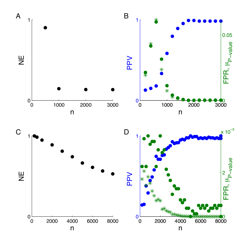
We now turn to the behavior of these performance metrics as a function of sample size. In the noiseless case (Figure 2A-B), the $NE$ showed a phase transition at $n\approx$ 1,000, but the $PPV$, $FPR$, and $\mu_{\textrm{$P$-value}}$ converged to zero around $n=$ 1,500. Since we fixed $s$ to be 125, the location of the transition boundary with respect to the $NE$ at the point ($\rho=0.125$, $\delta=0.125$) was consistent with Figure 1A. Also shown is the point ($\rho=0.08$, $\delta=0.19$), where the $PPV$, $FPR$, and $\mu_{\textrm{$P$-value}}$ converged to zero.

As the noise was increased (Figure 2C), the $NE$ declined less sharply with increasing $n$, as expected from Figure 1. In contrast as shown in Figure 2D, the other measures (particularly the $PPV$ and $\mu_{\textrm{$P$-value}}$) neared their asymptotic values even in the presence of noise. The transitions of $FPR$, $PPV$, and $\mu_{\textrm{$P$-value}}$ from poor to good performance were not smoothed by noise to the same extent as the transition of the $NE$.

The greater robustness of the $FPR$, $PPV$ and $\mu_{\textrm{$P$-value}}$ against residual variance relative to the $NE$ shows that accurate selection of nonzeros can occur well before the precise fitting of their coefficient magnitudes. The fact that the observable quantity $\mu_{\textrm{$P$-value}}$ exhibits this robustness is particularly important; a steep decline in $\mu_{\textrm{$P$-value}}$ across subsamples of increasing size drawn from a given dataset demonstrates a transition to good recovery and implies that the full dataset has sufficient power for accurate identification. This is an empirical finding which deserves further investigation.

For $h^{2}=0.5$ and across all measures of performance other than the $NE$, the transition appeared to be around $n=$ 5,000. Given $s=125$ and $p=$ 8,027, this corresponds to ($\rho=0.025$, $\delta=0.625$), which is circled in Figure 1B. This estimate of the critical $\rho$ is consistent with our previous estimate when $\delta$ was fixed at 0.5, supporting the weak dependence on $p$.

Quality of selection in the presence of LD

We have shown that randomly sampled SNPs from a GWAS of Europeans have the properties of a compressed sensor. This was expected, given that randomly sampled markers will be mostly uncorrelated and therefore closely approximate an isotropic matrix.

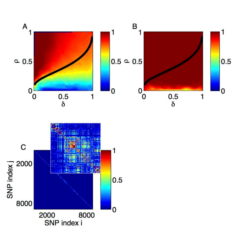
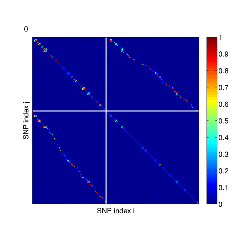
We next consider a genotype matrix characterized by LD. To do this while still being able to evaluate recovery at all points of the $\rho-\delta$ plane, we considered all genotyped markers on just chromosome 22. Almost all of these markers were in LD with a few other markers, and the markers within each correlated group tended to be spatially contiguous (Figure 3C). As shown in Figures 3A and 3B, the phase transition boundary with respect to $NE$ was shifted to lower values of $\rho$ and was less sensitive to $\delta$ as in the noisy case.

Although the phase transition from large to small $NE$ appeared to be affected adversely by LD (at least in the noiseless case as shown in Figure 3A), the selection measures were less affected, as seen by comparing Figure 4 calculated using the intact chromosome 22 with Figure 2 using markers drawn at random from across the genome. Regardless of LD, the transition from poor to good values of $\mu_{\textrm{$P$-value}}$ occurred at nearly the same sample size (about 30 times the number of nonzeros for $h^{2}=0.5$). The $PPV$ and $FPR$ saturated at worse asymptotic values in the noiseless case. In the noisy case, the $PPV$ was also lower; perhaps surprisingly, the $FPR$ actually increased with sample size.

The relatively poor performance of the $PPV$ and $FPR$ in the case of LD is somewhat misleading. For example, an “off-by-one” (nearby) nonzero called by $L_{1}$-penalized regression will not count toward the numerator of the $PPV$, even if it is in extremely strong LD with a true nonzero. At the same time, such a near miss does count toward the numerator of the $FPR$. This standard of recovery quality seems overly stringent when we recall that picking out the causal variant from a GWAS “hit” region containing multiple marker SNPs in LD continues to be a challenge for the standard MR approach maller:2012 ; edwards:2013 .

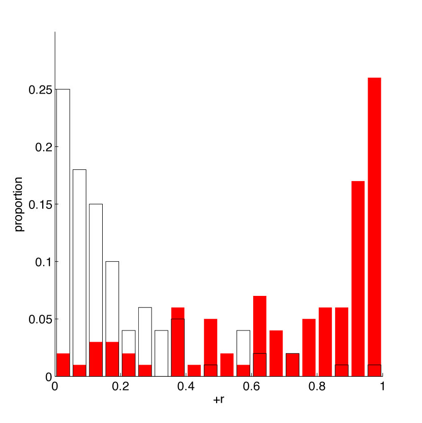
We examined whether the false positives called by the $L_{1}$-penalized algorithm were indeed more likely to be in strong LD with the true nonzeros by computing the correlations between false positives and true nonzeros for $n=$ 5,000 and $h^{2}=0.5$. Figure 5 shows the histogram of the maximum correlation between each false positive and any of the true nonzeros. We compared this histogram to a realization from the null distribution, generated by drawing markers at random from chromosome 22 and finding each such marker’s largest correlation with any of the true nonzeros. The observed histogram featured many more large correlations than the realization from the null distribution, implying that the false positives showed a significant tendency to be in LD with true nonzeros.

Figure 6 provides a visualization of the correlations among the false positives and true nonzeros. Both false positives and true nonzeros were sometimes in LD with neighboring members of their sets; this is to be expected given the short map length of chromosome 22. The small bursts of elevated color extending away from the diagonal of the upper-left quadrant suggest that false positives tend to occur in regions characterized by particularly strong LD. The striking feature of Figure 6 is the nearly continuous and isolated curve of elevated color slicing through the off-diagonal blocks of the correlation matrix. This curve shows that the between-set correlation structure was more complex than a one-to-one relationship assigning false positives to true nonzeros. Given the spatial ordering of the SNP indices, the linearity of the curve demonstrates a marked tendency for called false positives to occur close to one of the true nonzeros.

Sensitivity to the distributions of coefficient magnitudes and MAF

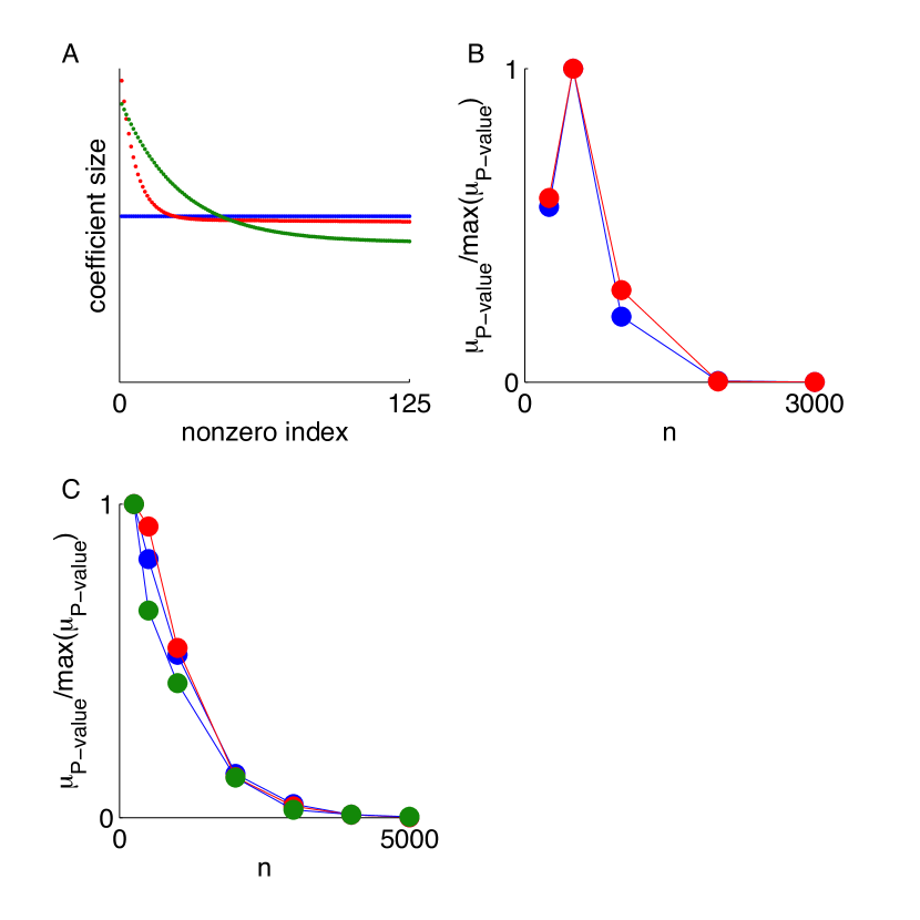
The appropriate prior on the distribution of coefficient magnitudes is often discussed gianola:2013:gs . However, CS theory shows that the phase boundary for complete selection is relatively insensitive to this distribution. To test this prediction, we looked for evidence of performance degradation upon replacing the discrete distribution of nonzero coefficients used thus far with a hyperexponential distribution (a mixture of exponential distributions with different decay constants) (these are defined in Data Description and shown in Figure 7A). The hyperexponential distribution is a means of implementing an arguably more realistic ensemble of a few large coefficients followed by a tail of weaker values chatterjee:2013 . Figure 7B-C shows that, as predicted by theoretical CS results, for fixed $h^{2}$ and chromosome 22, the normalized $\mu_{\textrm{$P$-value}}$ converged to zero at the same sample size regardless of the ensemble.

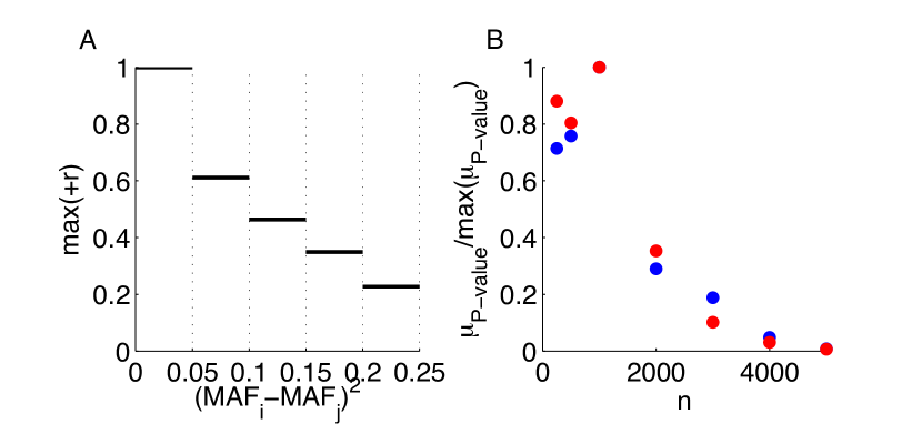
In the previous simulations, we drew the nonzeros at random from all genotyped markers, thus guaranteeing that the MAF spectra of the nonzeros and the entire genotyping chip would tend to coincide. Here, we also tested whether the MAF spectrum of nonzeros affects the selection phase boundary. It is known that two SNPs can be in strong LD only if they have similar MAFs hedrick:1987 ; wray:2011 . We confirmed this by taking all pairs of markers on chromosome 22 and plotting the maximum positive root of the LD measure as a function of squared MAF difference (Figure 8A). Therefore, in order to isolate any effect of the MAF distribution among nonzeros not mediated by LD, we constructed a synthetic measurement matrix $\mathbf{A}$ with independent columns and the same MAF spectrum as chromosome 22. We then compared recovery when the nonzero coefficients were sampled from SNPs with MAF between 0.0045 and 0.015 or when they were sampled above MAF of 0.49. For this we used nonzeros from $\{-1,1\}$. Figure 8B shows no difference in recovery between the conditions for $h^{2}=0.5$. This suggests that MAF alone is not a determinant of the phase transition. Homogeneity in MAF among nonzeros may enrich correlations as noted above. Such correlations would be expected to reduce the effective $s$ and thus affect the phase boundary.

Selection of SNPs associated with height

Motivated by the results above, we examined whether the full sample size of 12,454 subjects was sufficient to achieve the phase transition from poor to good recovery of SNPs associated with a real phenotype (height). We considered the selection measures $\mu_{\textrm{$P$-value}}$ and adjusted positive predictive value ($PPV^{*}$); the latter extended true-positive status to any selected SNP within 500 kb of a SNP identified as a likely marker of a height-affecting variant in the GIANT Consortium’s analysis of $\sim$180,000 unrelated individuals langoallen:2010 . This extension is consistent with the rule of thumb designating a 1-Mb region as a “locus” for purposes of counting the number of GWAS “hits” yang:2012:cond . The relative insensitivity of $\mu_{\textrm{$P$-value}}$ to LD suggests that $PPV^{*}$ rewards the identification of both true nonzeros and markers tagging nonzeros; we therefore substituted $PPV^{*}$ for $PPV$ in an attempt to align the phase dynamics of our precision measure with those of $\mu_{\textrm{$P$-value}}$. Whether a selected marker fell within 500 kb of a GIANT-identified marker was determined by consulting the the BROAD SNAP database (http://www.broadinstitute.org/mpg/snap/) johnson:2008:snap .

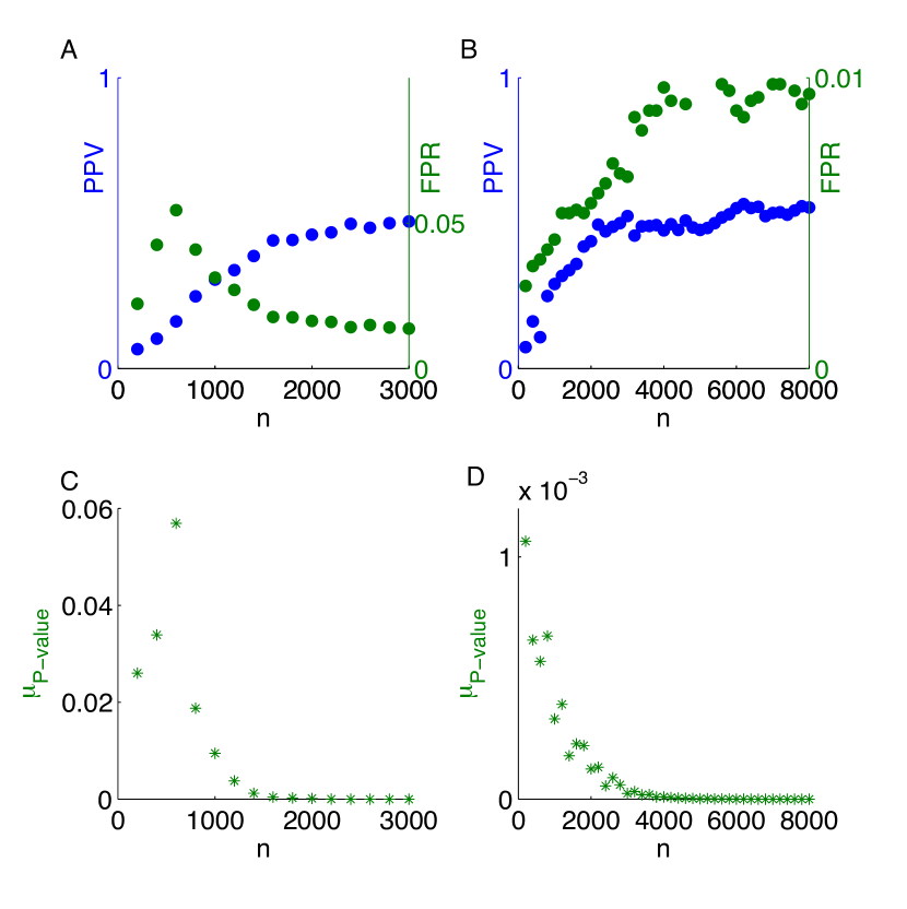
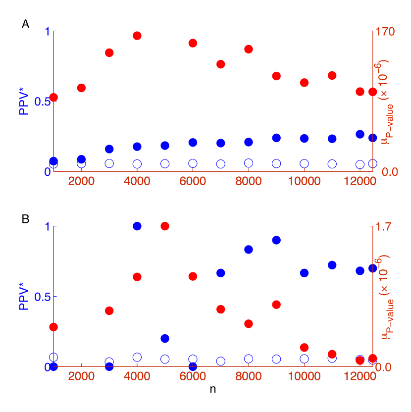
Figure 9A shows that $\mu_{\textrm{$P$-value}}$ failed to approach zero, suggesting that that $n=12,454$ is not large enough to see a phase transition to the regime of good recovery. Given our empirical finding that $\rho\approx 0.03$ is required for $h^{2}\approx 0.5$, this suggests that height is affected by at least 400 causal variants, a result consistent with the observation that the $\sim$250 known height-associated SNPs account for only a small proportion of this trait’s additive genetic variance yang:2012:cond . The null $PPV^{*}$ derived from randomly chosen SNPs, however, was smaller than the observed $PPV^{*}$ (Figure 9A); this was consistent with the detection of some true signal. In other words, although no phase transition was evident, the recovery measure did improve with increased sample size.

The penalization parameter $\lambda$ was set using CS theory to minimize NE error based on the expected noise-level from reported narrow sense heritability for height yang:2010:snpherit ; vattikuti:2012 . If $\lambda$ is set too low, then more false positives are expected; if $\lambda$ is set too high, then true nonzeros will be missed. According to CS theory, an $L_{1}$-penalized method can still select some of the largest coefficients from a nonuniform distribution of coefficient magnitudes even if complete recovery is out of reach candes:2006:stable . We investigated whether it was possible to achieve a phase transition to low $\mu_{\textrm{$P$-value}}$ and high $PPV^{*}$, at the cost of recovering only a small fraction of all true nonzeros, by increasing the penalty parameter $\lambda$. More specifically, we set $\lambda$ to a higher value consistent with $h^{2}=0.01$ rather than 0.5. In this case the $L_{1}$ algorithm returned 20 putative nonzeros rather than the original 403, and both $\mu_{\textrm{$P$-value}}$ and $PPV^{*}$ exhibited better performance (Figure 9B). Compared to the less stringent $\lambda$, $PPV^{*}$ as a function of $n$ was less smooth but appeared to stabilize to a high recovery value after $\sim 7000$ subjects. Evidently, if the sample size does not suffice to capture the full heritability, setting the penalty parameter to a value appropriate for a lower heritability can lead to a smaller set of selected markers characterized by good precision.

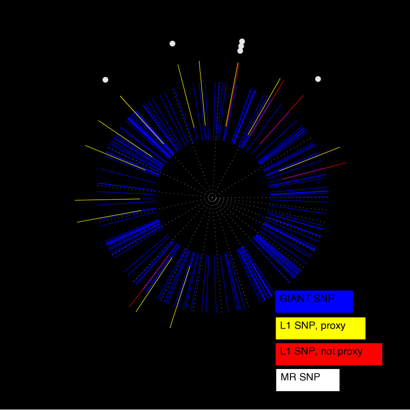
Figure 10 illustrates the physical distances between the markers selected in our strict-$\lambda$ (assuming $h^{2}=0.01$) analysis and the markers identified by the GIANT Consortium. Of the 20 $L_{1}$-selected markers, 14 were within 500-kb of a GIANT-identified marker. However, the $L_{1}$-selected markers defined to be false positives were still relatively close to GIANT-identified markers. This may indicate that the 500-kb criterion for declaring a true positive was too stringent; if so, then our stated $PPV^{*}$ of 0.7 can be regarded as a lower bound. As an informal comparison, Figure 10 also displays the results of a more standard MR-type GWAS analysis. For a $P$-value of $10^{-8}$ and all 12,454 subjects, MR returned six SNPs, five of which were GIANT-identified markers, and four were exact matches with SNPs selected by our $L_{1}$ algorithm (Figure 10). With a $P$-value cutoff of $5\times 10^{-8}$ and all subjects, MR returned 13 markers, 10 of which were GIANT-identified, and 7 of which were identical to the $L_{1}$-selected markers.

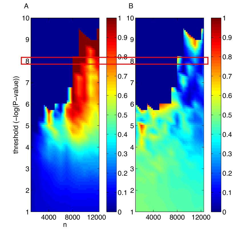
The presence of a phase transition is not necessarily restricted to $L_{1}$ algorithms but rather may represent a deeper phenomenon in signal recovery. Other methods may show a similar phase transition—although CS theory suggests that, among convex optimization methods, those within the $L_{1}$ class are closest to the optimal combinatorial $L_{0}$ search. We conducted additional analyses to test whether a phase transition at a critical sample size could also be observed when our height data were analyzed using the MR approach commonly used in GWAS. In these simulations we varied the $P$-value threshold for genome-wide significance. As measures of selection are potentially subject to a phase transition, we examined the $PPV^{*}$ and the adjusted median $P$-value ($\mu_{\textrm{$P$-value}}^{*}$). The latter measure was defined to be the median $P$-value among those SNPs surviving the $P$-value cutoff, divided by the cutoff itself; the normalization was necessary to remove the dependence on the choice of cutoff. As shown in Figure 11, the $P$-value threshold $10^{-8}$ yielded very few selected SNPs, and in fact none were returned at sample sizes smaller than about 8,000. However, $\mu_{\textrm{$P$-value}}^{*}$ was mostly close to zero in the region of Figure 11B corresponding to $n>8,000$ and $P\textrm{-value}<10^{-6}$, suggesting that true nonzeros were being selected. This is confirmed by the fact that the $PPV^{*}$ typically exceeded 0.6 in this same region (Figure 11A). For $P$-value thresholds less stringent than $10^{-6}$, signs of a phase transition at a critical sample size were still discernible.

A search for a phase transition can be a useful approach to determining the optimal $P$-value threshold in standard GWAS protocols employing MR. In addition to a priori assumptions regarding the likely number of true nonzeros and their coefficient magnitudes wtccc:2007 ; chatterjee:2013 and agreement between studies of different designs turchin:2012 , GWAS investigators might rely on whether a measure such as $\mu_{\textrm{$P$-value}}^{*}$ undergoes a clear phase transition as they take increasingly large subsamples of their data. A majority of markers surviving the most liberal significance threshold bounding the second phase are likely to be true positives.

Discussion

Our results with real European GWAS data and simulated vectors of regression coefficients demonstrate the accurate selection of those markers with nonzero coefficients, consistent with CS sample size requirements ($n$) for a given sparsity ($s$) and total number of predictors ($p$). We found that the matrix of standardized genotypes exhibits the theoretical phase transition between poor and complete selection of nonzeros (Proposition 1). We also found, as for Gaussian random matrices in earlier studies, that the phase transition depends on the scaling ratios $\rho=s/n$ and $\delta=n/p$ donoho:2010:precise .

We obtained results regarding the effect of noise (i.e., $h^{2}<1$) that are consistent with earlier empirical studies of random matrices and recently proven theorems donoho:2006:break ; donoho:2011 ; candes:2011:ripless . Roughly speaking, we show that the critical sample size is determined mainly by the ratio of $s$ to $n$ and only weakly sensitive to $p$, particularly as noise increases. For example, if $h^{2}=0.5$, which is roughly the narrow-sense heritability of height and a number of other quantitative traits yang:2010:snpherit ; davies:2011 ; vattikuti:2012 , we find that $\rho$ should be less than approximately 0.03 for recovery irrespective of $\delta$. There is no hope of recovering the complete vector of coefficients $\mathbf{x}$ above this threshold (i.e. smaller sample sizes). For example, if we have prior knowledge that $s=1,200$, then this means that the sample size should be no less than 40,000 subjects. We find empirically that for $h^{2}\sim 0.5$, $n\sim 30s$ is sufficient for selection of the nonzeros.

In real problems we cannot rely on measures of model recovery based on the unknown $\mathbf{x}$. Hence, we introduced a new measure based on the median $P$-value of the $L_{1}$-selected nonzeros, $\mu_{\textrm{$P$-value}}$. We found that $\mu_{\textrm{$P$-value}}$ provides a robust means of detecting the boundary between poor and good recovery. Proposition 2 shows that the recovery error $NE$ in the favorable phase scales with $\rho$ and noise; however, we observed that the recovery measures $FPR$, $PPV$ and $\mu_{\textrm{$P$-value}}$ approached zero faster than the $NE$, confirming that accurate identification of nonzeros can occur well before precise estimation of their magnitudes.

An $L_{1}$-penalized regression algorithm is equivalent to linear regression with a Laplace prior distribution of coefficients, and in theory a Bayesian method invoking a prior distribution better matching the unknown true distribution of nonzero coefficients should outperform the lasso in effect estimation. However, it is by no means clear that the performance of $L_{1}$ penalization with respect to selection can be bettered. For example, the lasso and BayesB display rather similar performance properties wimmer:2013 . However, both methods clearly outperformed ridge regression (a non-$L_{1}$ method), which exhibited no phase transition away from poor performance. Furthermore, it is usually accepted by GWAS researchers that knowledge of the markers with nonzero coefficients may be quite valuable, even if the actual magnitudes of the coefficients are not well determined. Combining the advantages of different approaches by applying one of them to the $L_{1}$-selected markers is a possibility.

Perhaps contrary to intuition, but consistent with theoretical results for CS donoho:2009 ; donoho:2010:precise , we found that the phase transition to good recovery (at least as measured by $\mu_{\textrm{$P$-value}}$) was insensitive to the distribution of coefficient magnitudes. It is well known in CS that $L_{1}$-penalized regression is nearly minimax optimal (minimizes the error of the worst case) and that the phase transition is robust to the distribution of coefficient magnitudes. In some cases a good prior may reduce the mean-square error and shift the location of the phase transition vila:2013 . Simulations supporting this notion, however, were performed with much higher signal-to-noise ratio (SNR) than hypothesized for realistic GWAS problems. The performance increase was attenuated as the SNR was decreased to levels still higher than usual in GWAS (10dB or $h^{2}>0.9$ where SNR on the dB scale is given by $10\cdot\log_{10}\left(\frac{\sigma^{2}_{A}}{\sigma^{2}_{E}}\right)$. These algorithms are currently being explored in lower-SNR regimes. We observed that cross-validation did slightly affect the phase transition boundary in the noisy case; nevertheless the theoretical penalization parameter proved to be a good “rule of thumb” for initial screening. Calculating the theoretical penalty depends on knowledge of $h^{2}$, which may be estimated using the genomic-relatedness method yang:2010:snpherit ; vattikuti:2012 ; vattikuti:2014 ; lee:2014 .

Genomic selection methods have been criticized by researchers who doubt that the number of nonzeros ($s$) will typically be smaller than a practically attainable sample size ($n$) gianola:2013:gs . The application of CS theory circumvents this problem because it allows the optimization method to self-determine whether or not the nonzero markers are sufficiently sparse compared to the sample size. No prior assumptions are required. Furthermore, in humans there is evidence that a number of traits satisfy the sparsity assumption, at least with respect to common variants contributing to heritability park:2011 ; stahl:2012 ; ripke:2013 .

CS theory does not provide performance guarantees in the presence of arbitrary correlations (LD) among predictor variables: it must be verified empirically, as we have done. In agreement with previous results wimmer:2013 , we find that the phase transition as measured by NE is strongly affected by LD. However, according to our simulations using all genotyped SNPs on chromosome 22, $L_{1}$-penalized regression does select SNPs in close proximity to true nonzeros. The difficulty of fine-mapping an association signal to the actual causal variant is a limitation shared by all statistical gene-mapping approaches—including marginal regression as implemented in standard GWAS—and thus should not be interpreted as a drawback of $L_{1}$ methods.

We found that a sample size of 12,464 was not sufficient to achieve full recovery of the nonzeros with respect to height. The penalization parameter $\lambda$, however, is set by CS theory so as to minimize the $NE$ based on the expected noise-level. In some situations it might be desirable to tolerate a relatively large $NE$ in order to achieve precise but incomplete recovery (few false positives, many false negatives). By setting $\lambda$ to a strict value appropriate for a low-heritability trait (in effect, looking for a subset of markers that account for only a fraction of the total heritability, with consequently higher noise), we found that a phase transition to good recovery can be achieved with smaller sample sizes, at the cost of selecting a smaller number of markers and hence suffering many false negatives.

One interesting feature of the recovery measure based on the median $P$-value ($\mu_{\textrm{$P$-value}}$) is that it seemed to rise as the sample size was increased in the region of poor recovery and then fall after the sample size crossed the CS-determined phase transition boundary. This rise and then fall was very dramatic in our simulations (Figures 2 and 4) and also appeared in our analysis of height (Figure 9). This behavior may be a consequence of the fact that as the sample size is increased, $\lambda$ in the algorithm is decreased (see Methods). Hence, in the region of poor recovery, the relaxation of the penalty with increasing sample size may permit the selection of more SNPs and hence the inflation of the $FPR$ and $\mu_{\textrm{$P$-value}}$. However, once the phase transition to good performance begins, the recovery measures begin their characteristic sharp decrease. This non-monotone behavior accentuates the transition boundary and can be exploited to aid its detection.

In summary, compressed sensing utilizes properties of high-dimensional systems that are surprising from the perspective of classical statistics. The regression problem faced by GWAS and GS is well-suited to such an approach, and we have shown that the matrix of SNP genotypes formed from European GWAS data is in fact a well-conditioned sensing matrix. Consequently, we have inferred the sample sizes required to achieve accurate model recovery and demonstrated a method for determining whether the minimal sample size has in fact been obtained.

Methods

$L_{1}$-penalized regression algorithm

$L_{1}$-penalized regression (e.g., lasso) minimizes the objective function

$$\|\hat{\mathbf{y}}-\mathbf{y}\|_{L_{2}}^{2}+\lambda\|\hat{\mathbf{x}}\|_{L_{1}}$$ (2)

where $\hat{\mathbf{y}}$ is the estimated breeding value given by $\mathbf{A}\hat{\mathbf{x}}$. The setting of the penalization parameter $\lambda$ is described below.

The algorithm was performed using pathwise coordinate optimization and the soft-threshold rule friedman:2007 . Regression coefficients were sequentially updated with

$$\hat{\mathbf{x}}_{j}(\lambda)\leftarrow S\left(\hat{\mathbf{x}}_{j}(\lambda)+\frac{1}{n}\sum\limits_{i=1}^{n}\mathbf{A}_{ij}(\mathbf{y}_{i}-\hat{\mathbf{y}}_{i}),\lambda\right)\textrm{ for }j=1,2,...,p$$ (3)

where

$$S\left(z,\lambda\right) \equiv \textrm{sign}(z)(|z|-\lambda)_{+}$$ (4)

$$= \begin{cases}z-\lambda,&\mbox{if }z>0\mbox{ and }\lambda<|z|,\\ z+\lambda,&\mbox{if }z<0\mbox{ and }\lambda<|z|,\\ 0,&\mbox{if }\lambda\geq|z|\\ \end{cases}$$

We assumed convergence if the fractional change in the objective function given by Equation 2 was less than $10^{-4}$. In addition, we performed lasso with a warm start friedman:2010 , using a logarithmic descent of 100 steps in $\lambda$ with $\lambda_{\textrm{max}}=(1/n)\|\mathbf{A}^{\prime}\mathbf{y}\|_{L_{\infty}}$. For $\lambda_{\textrm{min}}$ we used $(\sigma_{E}^{*}/n)\|\mathbf{A}^{\prime}\mathbf{e}\|_{L_{\infty}}$, where $\sigma_{E}^{*}=\sqrt{\sigma_{E}^{2}+1/n}$ candes:2011:ripless . To estimate $\|\mathbf{A}^{\prime}\mathbf{e}\|_{L_{\infty}}$ we created 1,000 sample vectors of $\mathbf{e}$, each constructed with $n$ i.i.d. normal elements with mean zero and variance one, and took the median across samples of $\|\mathbf{A}^{\prime}\mathbf{e}\|_{L_{\infty}}$ scaled by $\sigma_{E}^{*}$. Estimates of $(\sigma^{2}_{A},\sigma^{2}_{E})$ with respect to the variants assayed in a given study can be obtained using the genomic-relatedness method yang:2010:snpherit ; vattikuti:2012 ; vattikuti:2014 ; lee:2014 . The algorithm can also accommodate any other covariates.

Platform

Simulations and analyses were performed using MATLAB 2013 (The MathWorks Inc., Natick, Massachusetts) and PLINK 2 (https://www.cog-genomics.org/plink2/) purcell:2007 . The $L_{1}$-optimization algorithm was written in MATLAB (available at https://github.com/ShashaankV) and also a feature of PLINK 2. $P$-values were estimated using MATLAB’s regstats function and PLINK 2. Color-coded phase plane figures were generated by sampling the $\rho-\delta$ plane and interpolating between points using MATLAB’s scatteredInterpolant function. GWAS data were obtained from dbGaP as described in Data Description. Simulated mock data and the analysis scripts are available and maintained at https://github.com/ShashaankV.

Statistics

The normalized coefficient error ($NE$) is

$$\dfrac{\|x-\hat{x}\|_{L_{2}}}{\|x\|_{L_{2}}}.$$ (5)

The false positive rate ($FPR$) is the fraction of true zero-valued coefficients that are falsely identified as nonzero. The positive predictive value ($PPV$) is the number of correctly selected true nonzeros divided by the total number of nonzeros returned by the selection algorithm. $1-PPV$ equals the false discovery rate ($FDR$). The adjusted positive predictive value ($PPV^{*}$) is similar to the standard $PPV$, except that any selected nonzero coefficient falling within 500 kb of a GIANT-identified marker is counted as a true positive langoallen:2010 .

The median of the $P$-values for the set of putative nonzeros ($\mu_{P-value}$) is obtained by: 1) regressing the phenotype on each of the $L_{1}$-selected markers in turn, 2) estimating each $P$-value as the standard two-tailed probability from the $t$ test of the null hypothesis that a univariate regression coefficient is equal to zero, and 3) taking the median over the independent tests. This procedure is independent of the selection algorithm and calculated after the $L_{1}$-penalized algorithm has converged. The adjusted median $P$-value ($\mu_{\textrm{$P$-value}}^{*}$) is the median of the MR $P$-values falling below the significance threshold divided by the threshold itself.

The LD measure ($r^{2}$) is the squared estimate of the Pearson’s product-moment correlation between the standardized zero-mean, unit-variance SNPs.

As noted above the raw data is available through dbGaP. Mock data and the analysis codes are available and maintained at https://github.com/ShashaankV.

Abbreviations

ARIC: Atherosclerosis Risk in Community; CS: compressed sensing; FDR: false discovery rate; FPR: false positive rate; GENEVA: Gene Environment Association Studies; GIANT: Genetic Investigation of Anthropometric Traits; GS: genomic selection; GWAS: genome-wide association study; LD: linkage disequilibrium; LE: linkage equilibrium; MAF: minor allele frequency; MR: marginal regression; NE: normalized error; OLS: ordinary least squares; PPV: positive predictive value; SNP: single-nucleotide polymorphism.

Competing interests

The authors declare that they have no competing interests.

Author’s contributions

SV performed the numerical experiments and analyzed the data. SV, JJL, SDHH, and Chow contributed to the conception of the study, drafted the article, and endorsed the final version for submission. Chang ported the MATLAB $L_{1}$-penalized regression codes to PLINK 2 for use in the height analysis.

Figures

Figure 1: Error in the $\rho-\delta$ plane for a measurement matrix of random genomic SNPs ($\rho=s/n$ and $\delta=n/p$). (A) Color corresponds to the normalized error ($NE$) of the coefficients $\dfrac{\|x-\hat{x}\|_{L_{2}}}{\|x\|_{L_{2}}}$. The black curve is the expected phase boundary between poor and good recovery from donoho:2006:neighbor . The number of SNPs, $p$, was fixed at 8,027. The heritability was set to one (noiseless case). The circles correspond to the points ($\rho=0.08$, $\delta=0.19$) (white) and ($\rho=0.125$, $\delta=0.125$) (red) discussed in Measures of selection. (B) Same as panel (A), except that the heritability was set to 0.5 (noisy case). The white circle corresponds to the point ($\rho=0.025$, $\delta=0.625$) discussed in Measures of selection. (C) $NE$ versus $\rho$ for fixed $n=$ 4,000 and $p=$ 8,027 (blue corresponds to $h^{2}=1$, red to $h^{2}=0.5$). The square markers indicate recovery quality evaluated at a few data points using the lasso algorithm with 10-fold cross-validation written by MATLAB.

Figure 2: Measures of selection as a function of sample size for the measurement matrix of random genomic SNPs. Fixing $s=125$ and $p=$ 8,027, we measured the selection of true nonzero coefficients according to four metrics for $h^{2}=1$ (A-B) and $h^{2}=0.5$ (C-D). Shown in (A-C) is the normalized error of the coefficients ($NE$). Shown in (B-D) are the positive predictive value ($PPV$, blue dots), false positive rate ($FPR$, green dots), and median $P$-value ($\mu_{\textrm{$P$-value}}$, green asterisks). The point $n=1,000$ corresponds to ($\rho=0.125$, $\delta=0.125$) and $n=5,000$ to ($\rho=0.025$, $\delta=0.625$) noted in Figures 1 A and B respectively.

Figure 3: Analysis of chromosome 22. (A) The $\rho-\delta$ plane for $h^{2}=1$. $p$ was set to 8,915. Superimposed is the expected phase boundary when there is neither noise nor LD. (B) The same as panel (A), except for $h^{2}=0.5$. (C) The matrix of correlations (positive roots of the $r^{2}$ LD measure) between genotyped SNPs on chromosome 22. Inset is a $100\times 100$ sample along the diagonal.

Figure 4: Measures of selection as a function of sample size for chromosome 22 ($s=125$ and $p=8,915$). The PPV (blue) and FPR (green) for $h^{2}=1$ (A) and $h^{2}=0.5$ (B). $\mu_{P-value}$ for $h^{2}=1$ (C) and $h^{2}=0.5$ (D).

Figure 5: Distribution of maximum correlations between false positives and true nonzeros after the presumptive $\mu_{P-value}$ phase transition for chromosome 22. Histogram of the maximum correlation (maximum of the positive roots of the $r^{2}$ LD measure) between a false positive and true nonzero for chromosome 22, given $s=125$, $n=$ 5,000, and $h^{2}=0.5$ (red). Also shown is one realization from the null distribution, generated by drawing an equal number of “false positives” at random from chromosome 22 (white).

Figure 6: The matrix of correlations (positive roots of the $r^{2}$ LD measure) among false positives and true nonzeros after the presumptive $\mu_{P-value}$ phase transition for chromosome 22 ($s=125$, $n=5,000$, and $h^{2}=0.5$). SNP indices begin at the top left corner. The upper-left quadrant contains the correlations among false positives and the lower-right quadrant contains the correlations among the true nonzeros. Each element in the upper-right (lower-left) quadrant represents a correlation between a false positive and a true nonzero. Within both the false positive and the true nonzero sets, the markers are arranged in order of chromosomal map position.

Figure 7: Insensitivity of the selection phase boundary to the distribution of coefficient magnitudes (ensemble). (A) $s=125$ coefficient magnitudes (“effect sizes”) ordered from large to small for the Uniform (blue), Hyperexponential 1 (red), and Hyperexponential 2 (green) ensembles. (B) Chromosome 22 analysis using $\mu_{\textrm{$P$-value}}$ to measure selection (normalized by the maximum value) as a function of sample size for $h^{2}=1$ for the Uniform (blue) and Hyperexponential 1 (red) ensembles. (C) As in panel (B) except for $h^{2}=0.5$. Also shown is recovery for the Hyperexponential 2 ensemble (green).

Figure 8: Insensitivity of the selection phase boundary to minor allele frequency (MAF) for chromosome 22. (A) The maximum positive root of the $r^{2}$ LD measure (+r) as a function of squared MAF difference. The maxima are estimated over bin lengths of 0.05 for SNPs in chromosome 22. (B) The median $P$-value ($\mu_{\textrm{$P$-value}}$) normalized by the maximum value as a function of sample size for $s=125$ from $\{-1,1\}$ and $h^{2}=0.5$ for nonzero coefficients sampled from low (blue) or high (red) MAF SNPs on chromosome 22.

Figure 9: Selection measures as a function of sample size in an analysis of real height data. (A) The adjusted positive predictive value ($PPV^{*}$, blue solid dots) and median $P$-value ($\mu_{\textrm{$P$-value}}$, red) as a function of sample size using $\lambda$ based on $h^{2}=0.5$. Also shown is $PPV^{*}$ when the same number of SNPs are randomly selected rather than returned by the $L_{1}$ algorithm (blue unfilled dots). (B) As in (A) but setting $\lambda$ to a value appropriate for $h^{2}=0.01$.

Figure 10: Map of SNPs associated with height, as identified by the GIANT Consortium meta-analysis, $L_{1}$-penalized regression, and standard GWAS. Base-pair distance is given by angle, and chromosome endpoints are demarcated by dotted lines. Starting from 3 o’clock and going counterclockwise, the map sweeps through the chromosomes in numerical order. As a scale reference, the first sector represents chromosome 1 and is $\sim$ 250 million base-pairs. The blue segments correspond to a 1Mb window surrounding the height-associated SNPs discovered by GIANT. Note that some of these may overlap. The yellow segments represent $L_{1}$-selected SNPs that fell within 500 kb of a (blue) GIANT-identified nonzero; these met our criterion for being declared true positives. The red segments represent $L_{1}$-selected SNPs that did not fall within 500 kb of a GIANT-identified nonzero. Note that some yellow and red segments overlap given this figure’s resolution. There are in total 20 yellow/red segments, representing $L_{1}$-selected SNPs found using all 12,454 subjects. The white dots represent the locations of SNPs selected by MR at a $P$-value threshold of $10^{-8}$.

Figure 11: Measures of recovery using marginal regression (standard GWAS) as a function of sample size. All SNPs surviving the chosen $-\log_{10}P\textrm{-value}$ threshold were selected. The recovery measures, computed over the selected SNPs, were (A) the adjusted positive predictive value ($PPV^{*}$) and (B) the median $P$-value divided by the $P$-value cutoff. Highlighted in red is the cutoff we used for MR in Figure 10.

References

- (1) Johnstone, I.M., Titterington, D.M.: Statistical challenges of high-dimensional data. Philos Trans R Soc A 367(1906), 4237–4253 (2009)
- (2) Hoggart, C.J., Whittaker, J.C., De Iorio, M., Balding, D.J.: Simultaneous analysis of all SNPs in genome-wide and re-sequencing association studies. PLoS Genet 4(7), 1000130 (2008)
- (3) Goddard, M.E., Wray, N.R., Verbyla, K., Visscher, P.M.: Estimating effects and making predictions from genome-wide marker data. Stat Sci 24(4), 517–529 (2009)
- (4) Kemper, K.E., Daetwyler, H.D., Visscher, P.M., Goddard, M.E.: Comparing linkage and association analyses in sheep points to a better way of doing GWAS. Genet Res 94(4), 191–203 (2012)
- (5) Genovese, C.R., Jin, J., Wasserman, L., Yao, Z.: A comparison of the lasso and marginal regression. J Mach Learn Res 13(1), 2107–2143 (2012)
- (6) Visscher, P.M., Brown, M.A., McCarthy, M.I., Yang, J.: Five years of GWAS discovery. Am J Hum Genet 90(1), 7–24 (2012)
- (7) Yang, J., Benyamin, B., McEvoy, B.P., Gordon, S., Henders, A.K., Nyholt, D.R., Madden, P.A., Heath, A.C., Martin, N.G., Montgomery, G.W., Goddard, M.E., Visscher, P.M.: Common SNPs explain a large proportion of the heritability for human height. Nat Genet 42(7), 565–569 (2010)
- (8) Tibshirani, R.: Regression shrinkage and selection via the lasso. J Roy Stat Soc B 58(1), 267–288 (1996)
- (9) Park, J.-H., Gail, M.H., Weinberg, C.R., Carroll, R.J., Chung, C.C., Wang, Z., Chanock, S.J., Fraumeni, J.F., Chatterjee, N.: Distribution of allele frequencies and effect sizes and their interrelationships for common genetic susceptibility variants. Proc Natl Acad Sci USA 108(44), 18026–18031 (2011)
- (10) Stahl, E.A., Wegmann, D., Trynka, G., Gutierrez-Achury, J., Do, R., Voight, B.F., Kraft, P., Chen, R., Kallberg, H.J., Kurreeman, F.A.S., Diabetes Genetics Replication and Meta-Analysis Consortium, Myocardial Infarction Genetics Consortium, Kathiresan, S., Wijmenga, C., Gregersen, P.K., Alfredsson, L., Siminovitch, K.A., Worthington, J., de Bakker, P.I.W., Raychaudhuri, S., Plenge, R.M.: Bayesian inference analyses of the polygenic architecture of rheumatoid arthritis. Nat Genet 44(5), 483–489 (2012)
- (11) Ripke, S., O’Dushlaine, C., Chambert, K., Moran, J.L., Kähler, A.K., Akterin, S., Bergen, S.E., Collins, A.L., Crowley, J.J., Fromer, M., Kim, Y., Lee, S.H., Magnusson, P.K.E., Sanchez, N., Stahl, E.A., Williams, S., Wray, N.R., Xia, K., Bettella, F., Børglum, A.D., Bulik-Sullivan, B.K., Cormican, P., Craddock, N., de Leeuw, C., Durmishi, N., Gill, M., Golimbet, V., Hamshere, M.L., Holmans, P., Hougaard, D.M., Kendler, K.S., Lin, K., Morris, D.W., Mors, O., Mortensen, P.B., Neale, B.M., O’Neill, F.A., Owen, M.J., Milovancevic, M.P., Posthuma, D., Powell, J., Richards, A.L., Riley, B.P., Ruderfer, D.M., Rujescu, D., Sigurdsson, E., Silagadze, T., Smit, A.B., Stefansson, H., Steinberg, S., Suvisaari, J., Tosato, S., Verhage, M., Walters, J.T., Bramon, E., Corvin, A.P., O’Donovan, M.C., Stefansson, K., Scolnick, E., Purcell, S.M., McCarroll, S.A., Sklar, P., Hultman, C.M., Sullivan, P.F.: Genome-wide association analysis identifies 13 new risk loci for schizophrenia. Nat Genet 45(10), 1150–1159 (2013)
- (12) Meuwissen, T.H.E., Hayes, B.J., Goddard, M.E.: Prediction of total genetic value using genome-wide dense marker maps. Genetics 157(4), 1819–1829 (2001)
- (13) de los Campos, G., Gianola, D., Allison, D.B.: Predicting genetic predisposition in humans: The promise of whole-genome markers. Nat Rev Genet 11(12), 880–886 (2010)
- (14) Hayes, B.J., Pryce, J., Chamberlain, A.J., Bowman, P.J., Goddard, M.E.: Genetic architecture of complex traits and accuracy of genomic prediction: Coat colour, milk-fat percentage, and type in Holstein cattle as contrasting model traits. PLoS Genet 6(9), 1001139 (2010)
- (15) Meuwissen, T.H.E., Hayes, B.J., Goddard, M.E.: Accelerating improvement of livestock with genomic selection. Annu Rev Anim Biosci 1(1), 221–237 (2013)
- (16) Usai, M.G., Goddard, M.E., Hayes, B.J.: LASSO with cross-validation for genomic selection. Genet Res 91(6), 427–436 (2009)
- (17) Wimmer, V., Lehermeier, C., Albrecht, T., Auinger, H.-J., Wang, Y., Schön, C.-C.: Genome-wide prediction of traits with different genetic architecture through efficient variable selection. Genetics 195(2), 573–587 (2013)
- (18) Zhou, X., Carbonetto, P., Stephens, M.: Polygenic modeling with Bayesian sparse linear mixed models. PLoS Genet 9(2), 1003264 (2013)
- (19) Gianola, D.: Priors in whole-genome regression: The Bayesian alphabet returns. Genetics 194(3), 573–596 (2013)
- (20) Donoho, D.L., Tanner, J.: Sparse nonnegative solution of underdetermined linear equations by linear programming. Proc Natl Acad Sci USA 102(27), 9446–9451 (2005)
- (21) Candès, E.J., Plan, Y.: Near-ideal model selection by minimization. Ann Stat 37(5A), 2145–2177 (2009)
- (22) Candès, E.J., Plan, Y.: A probabilistic and RIPless theory of compressed sensing. IEEE Trans Inform Theory 57(11), 7235–7254 (2011)
- (23) Candès, E.J., Romberg, J., Tao, T.: Robust uncertainty principles: Exact signal reconstruction from highly incomplete frequency information. IEEE Trans Inform Theory 52(2), 489–509 (2006)
- (24) Donoho, D.L., Maleki, A., Montanari, A.: The noise-sensitivity phase transition in compressed sensing. IEEE Trans Inform Theory 57, 6920–6941 (2011)
- (25) Donoho, D.L., Maleki, A., Montanari, A.: Message-passing algorithms for compressed sensing. Proc Natl Acad Sci USA 106(45), 18914–18919 (2009)
- (26) Donoho, D.L.: High-dimensional centrally symmetric polytopes with neighborliness proportional to dimension. Discrete Comput Geom 35(4), 617–652 (2006)
- (27) Donoho, D., Tanner, J.: Observed universality of phase transitions in high-dimensional geometry, with implications for modern data analysis and signal processing. Philos Trans A Math Phys Eng Sci 367(1906), 4273–93 (2009)
- (28) Donoho, D.L., Stodden, V.: Breakdown Point of Model Selection When the Number of Variables Exceeds the Number of Observations. In: International Joint Conference on Neural Networks, Vancouver, Canada, pp. 1916–1921 (2006)
- (29) Monajemi, H., Jafarpour, S., Gavish, M., Stat 330/CME 362 Collaboration, Donoho, D.L.: Deterministic matrices matching the compressed sensing phase transition of Gaussian random matrices. Proc Natl Acad Sci USA 110(4), 1181–1186 (2013)
- (30) Vattikuti, S., Guo, J., Chow, C.C.: Heritability and genetic correlations explained by common SNPs for metabolic syndrome traits. PLoS Genet 8(3) (2012)
- (31) Vattikuti, S., Chow, C.C.: Software: Heritability and genetic correlations explained by common SNPs for metabolic syndrome traits. https://github.com/ShashaankV/MVLME/
- (32) Lee, J.J., Chow, C.C.: Conditions for the validity of snp-based heritability estimation. Human Genetics (2014)
- (33) Johnstone, I.: Oracle inequalities and nonparametric function estimation. Department of Statistics, Stanford University (1998)
- (34) Purcell, S.M., Neale, B.M., Todd-Brown, K., Thomas, L., Ferreira, M.A.R., Bender, D., Maller, J., Sklar, P., de Bakker, P.I.W., Daly, M.J., Sham, P.C.: PLINK: A tool set for whole-genome association and population-based linkage analyses. Am J Hum Genet 81, 559–575 (2007)
- (35) Davies, G., Tenesa, A., Payton, A., Yang, J., Harris, S.E., Goddard, M.E., Liewald, D., Ke, X., Le Hellard, S., Christoforou, A., Luciano, M., McGhee, K.A., Lopez, L.M., Gow, A.J., Corley, J., Redmond, P., Fox, H.C., Haggarty, P., Whalley, L.J., McNeill, G., Espeseth, T., Lundervold, A.J., Reinvang, I., Pickles, A., Steen, V.M., Ollier, W., Porteous, D.J., Horan, M.A., Starr, J.M., Pendleton, N., Visscher, P.M., Deary, I.J.: Genome-wide association studies establish that human intelligence is highly heritable and polygenic. Mol Psychiatry 16(10), 996–1005 (2011)
- (36) Chatterjee, N., Wheeler, B., Sampson, J., Hartge, P., Chanock, S.J., Park, J.-H.: Projecting the performance of risk prediction based on polygenic analyses of genome-wide association studies. Nat Genet 45(4), 400–405 (2013)
- (37) Lango Allen, H., Estrada, K., Lettre, G., Berndt, S.I., Weedon, M.N., Rivadeneira, F., Willer, C.J., Jackson, A.U., Vedantam, S., Raychaudhuri, S., Ferreira, T., Wood, A.R., Weyant, R.J., Segre, A.V., Speliotes, E.K., Wheeler, E., Soranzo, N., Park, J.-H., Yang, J., Gudbjartsson, D., Heard-Costa, N.L., Randall, J.C., Qi, L., Vernon Smith, A., Magi, R., Pastinen, T., Liang, L., Heid, I.M., Luan, J., Thorleifsson, G., Winkler, T.W., Goddard, M.E., Sin Lo, K., Palmer, C., Workalemahu, T., Aulchenko, Y.S., Johansson, A., Carola Zillikens, M., Feitosa, M.F., Esko, T., Johnson, T., Ketkar, S., Kraft, P., Mangino, M., Prokopenko, I., Absher, D., Albrecht, E., Ernst, F., Glazer, N.L., Hayward, C., Hottenga, J.-J., Jacobs, K.B., Knowles, J.W., Kutalik, Z., Monda, K.L., Polasek, O., Preuss, M., Rayner, N.W., Robertson, N.R., Steinthorsdottir, V., Tyrer, J.P., Voight, B.F., Wiklund, F., Xu, J., Hua Zhao, J., Nyholt, D.R., Pellikka, N., Perola, M., Perry, J.R.B., Surakka, I., Tammesoo, M.-L., Altmaier, E.L., Amin, N., Aspelund, T., Bhangale, T., Boucher, G., Chasman, D.I., Chen, C., Coin, L., Cooper, M.N., Dixon, A.L., Gibson, Q., Grundberg, E., Hao, K., Juhani Junttila, M., Kaplan, L.M., Kettunen, J., Konig, I.R., Kwan, T., Lawrence, R.W., Levinson, D.F., Lorentzon, M., McKnight, B., Morris, A.P., Muller, M., Suh Ngwa, J., Purcell, S., Rafelt, S., Salem, R.M., Salvi, E., Sanna, S., Shi, J., Sovio, U., Thompson, J.R., Turchin, M.C., Vandenput, L., Verlaan, D.J., Vitart, V., White, C.C., Ziegler, A., Almgren, P., Balmforth, A.J., Campbell, H., Citterio, L., De Grandi, A., Dominiczak, A., Duan, J., Elliott, P., Elosua, R., Eriksson, J.G., Freimer, N.B., Geus, E.J.C., Glorioso, N., Haiqing, S., Hartikainen, A.-L., Havulinna, A.S., Hicks, A.A., Hui, J., Igl, W., Illig, T., Jula, A., Kajantie, E., Kilpelainen, T.O., Koiranen, M., Kolcic, I., Koskinen, S., Kovacs, P., Laitinen, J., Liu, J., Lokki, M.-L., Marusic, A., Maschio, A., Meitinger, T., Mulas, A., Pare, G., Parker, A.N., Peden, J.F., Petersmann, A., Pichler, I., Pietilainen, K.H., Pouta, A., Ridderstrale, M., Rotter, J.I., Sambrook, J.G., Sanders, A.R., Oliver Schmidt, C., Sinisalo, J., Smit, J.H., Stringham, H.M., Bragi Walters, G., Widen, E., Wild, S.H., Willemsen, G., Zagato, L., Zgaga, L., Zitting, P., Alavere, H., Farrall, M., McArdle, W.L., Nelis, M., Peters, M.J., Ripatti, S., van Meurs, J.B.J., Aben, K.K., Ardlie, K.G., Beckmann, J.S., Beilby, J.P., Bergman, R.N., Bergmann, S., Collins, F.S., Cusi, D., den Heijer, M., Eiriksdottir, G., Gejman, P.V., Hall, A.S., Hamsten, A., Huikuri, H.V., Iribarren, C., Kahonen, M., Kaprio, J., Kathiresan, S., Kiemeney, L., Kocher, T., Launer, L.J., Lehtimaki, T., Melander, O., Mosley Jr, T.H., Musk, A.W., Nieminen, M.S., O/’Donnell, C.J., Ohlsson, C., Oostra, B., Palmer, L.J., Raitakari, O., Ridker, P.M., Rioux, J.D., Rissanen, A., Rivolta, C., Schunkert, H., Shuldiner, A.R., Siscovick, D.S., Stumvoll, M., Tonjes, A., Tuomilehto, J., van Ommen, G.-J., Viikari, J., Heath, A.C., Martin, N.G., Montgomery, G.W., Province, M.A., Kayser, M., Arnold, A.M., Atwood, L.D., Boerwinkle, E., Chanock, S.J., Deloukas, P., Gieger, C., Gronberg, H., Hall, P., Hattersley, A.T., Hengstenberg, C., Hoffman, W.: Hundreds of variants clustered in genomic loci and biological pathways affect human height. Nature 467(7317), 832–838 (2010)
- (38) Johnson, A.D., Handsaker, R.E., Pulit, S.L., Nizzari, M.M., O’Donnell, C.J., de Bakker, P.I.W.: SNAP: A web-based tool for identification and annotation of proxy SNPs using HapMap. Bioinformatics 24(24), 2938–2939 (2008)
- (39) Abraham, G., Kowalczyk, A., Zobel, J., Inouye, M.: Performance and robustness of penalized and unpenalized methods for genetic prediction of complex human disease. Genet Epidemiol 37(2), 184–195 (2013)
- (40) Donoho, D.L., Tanner, J.: Precise undersampling theorems. Proc IEEE 98(6), 913–924 (2010)
- (41) Storey, J., Tibshirani, R.: Statistical significance for genome-wide studies. Proceedings of the National Academy of Sciences 100, 9440–9445 (2003)
- (42) Maller, J.B., McVean, G., Byrnes, J., Vukcevic, D., Palin, K., Su, Z., Howson, J.M.M., Auton, A., Myers, S., Morris, A., Pirinen, M., Brown, M.A., Burton, P.R., Caulfield, M.J., Compston, A., Farrall, M., Hall, A.S., Hattersley, A.T., Hill, A.V.S., Mathew, C.G., Pembrey, M., Satsangi, J., Stratton, M.R., Worthington, J., Craddock, N., Hurles, M., Ouwehand, W.H., Parkes, M., Rahman, N., Duncanson, A., Todd, J.A., Kwiatkowski, D.P., Samani, N.J., Gough, S.C.L., McCarthy, M.I., Deloukas, P., Donnelly, P.: Bayesian refinement of association signals for 14 loci in 3 common diseases. Nat Genet 44(12), 1294–1301 (2012)
- (43) Edwards, S.L., Beesley, J., French, J.D., Dunning, A.M.: Beyond GWASs: Illuminating the dark road from association to function. Am J Hum Genet 93(5), 779–797 (2013)
- (44) Hedrick, P.W.: Gametic disequilibrium measures: proceed with caution. Genetics 117(2), 331–41 (1987)
- (45) Wray, N.R., Purcell, S.M., Visscher, P.M.: Synthetic associations created by rare variants do not explain most GWAS results. PLoS Biology 9(1), 1000579 (2011)
- (46) Yang, J., Ferreira, T., Morris, A.P., Medland, S.E., Genetic Investigation of Anthropometric Traits Consortium, Diabetes Genetics Replication and Meta-Analysis Consortium, Madden, P.A.F., Heath, A.C., Martin, N.G., Montgomery, G.W., Weedon, M.N., Loos, R.J., Frayling, T.M., McCarthy, M.I., Hirschhorn, J.N., Goddard, M.E., Visscher, P.M.: Conditional and joint multiple-SNP analysis of GWAS summary statistics identifies additional variants influencing complex traits. Nat Genet 44(4), 369–375 (2012)
- (47) Candès, E.J., Romberg, J.K., Tao, T.: Stable signal recovery from incomplete and inaccurate measurements. Commun Pure Appl Math 59(8), 1207–1223 (2006)
- (48) Wellcome Trust Case Control Consortium: Genome-wide association study of 14,000 cases of seven common diseases and 3,000 shared controls. Nature 447(7145), 661–678 (2007)
- (49) Turchin, M.C., Chiang, C.W.K., Palmer, C.D., Sankararaman, S., Reich, D., Genetic Investigation of Anthropometric Traits Consortium, Hirschhorn, J.N.: Evidence of widespread selection on standing variation in Europe at height-associated SNPs. Nat Genet 44(9), 1015–1019 (2012)
- (50) Vila, J., Schniter, P.: Expectation-maximization gaussian-mixture approximate message passing. IEEE Trans. Signal Process 61, 4858–4672 (2013)
- (51) Friedman, J., Hastie, T., Höfling, H., Tibshirani, R.: Pathwise coordinate optimization. Ann Appl Stat 1(2), 302–332 (2007)
- (52) Friedman, J., Hastie, T., Tibshirani, R.: Regularization paths for generalized linear models via coordinate descent. J Stat Softw 33(1), 1–22 (2010)