The application of the exact operational matrices for solving
the Emden-Fowler equations, arising in astrophysics

K. Parand {}^{\mbox{\footnotesize}}  , Sayyed A. Hossayni{}^{\mbox{\footnotesize}}  , J.A. Rad{}^{\mbox{\footnotesize}}

aa{}^{\mbox{\footnotesize a}}Department of Computer Sciences, Faculty of Mathematical Sciences,
Shahid Beheshti University, Evin,Tehran 19839,Iran
E-mail address: k_parand@sbu.ac.ir, Corresponding author, (K. Parand)E-mail address: hossayni@iran.ir, (Sayyed A. Hossayni)E-mail address: j.amanirad@gmail.com; j_amanirad@sbu.ac.ir, (J.A. Rad)
Abstract

The objective of this paper is to apply the well-known exact operational matrices (EOMs) idea for solving the Emden-Fowler equations, illustrating the superiority of EOMs versus ordinary operational matrices (OOMs). Up to now, a few studies have been conducted on EOMs and the differential equations solved by them do not have high-degree nonlinearity and the reported results are not regarded as appropriate criteria for the excellence of the new method. So, we chose Emden-Fowler type differential equations and solved them by this method. To confirm the accuracy of the new method and to show the preeminence of EOMs versus OOMs, the norm1 of the residual and error function of both methods are evaluated for multiple m𝑚m values, where m𝑚m is the degree of the Bernstein polynomials. We reported the results in form of plots to illustrate the error convergence of both methods to zero and also to show the primacy of the new method versus OOMs. The obtained results have demonstrated the increased accuracy of the new method.

Keywords: Exact operational matrices, Bernstein polynomials, Emden-Fowler equation, Lane-Emden equation.

AMS subject classification: 65M70, 65N35.

1 Introduction

In 1915, Galerkin [1] introduced a broad generalization of the Ritz [2] method to be used primarily for the approximate solution of variational and boundary value problems, including problems that cannot be reduced to variational problems [3]. His method was highly appreciated and thousands of problems have been solved, using the Galerkin method, since 1915.
The basic idea behind the Galerkin method is as follows. Suppose it is required to find a solution, defined in some domain U𝑈U, of the following (nonlinear) differential equation (which does not have any exact analytical solution)

𝒩[u(x)]=0,𝒩delimited-[]𝑢𝑥0\displaystyle\mathcal{N}\left[u(x)\right]=0, xU𝑥𝑈\displaystyle x\in U (1)
B(u(s))=0,𝐵𝑢𝑠0\displaystyle B\left(u(s)\right)=0, sU𝑠𝑈\displaystyle s\in\partial U

where the solution satisfies at the boundary B(u(s))𝐵𝑢𝑠B\left(u(s)\right) of U𝑈U the homogeneous boundary conditions. Firstly, suppose arbitrary so-called ”trial” functions βi(x)subscript𝛽𝑖𝑥\beta_{i}(x)

u(x)ym(x)=i=0ciβi(x)𝑢𝑥subscript𝑦𝑚𝑥superscriptsubscript𝑖0subscript𝑐𝑖subscript𝛽𝑖𝑥\displaystyle u(x)\approx y_{m}(x)=\sum_{i=0}^{\infty}{c_{i}\beta_{i}(x)} B(ym(s))=0,𝐵subscript𝑦𝑚𝑠0\displaystyle B\left(y_{m}(s)\right)=0, sU𝑠𝑈\displaystyle s\in\partial U (2)

As we mentioned, 𝒩[u(x)]𝒩delimited-[]𝑢𝑥\mathcal{N}\left[u(x)\right] does not have any exact analytical solution; so, we are sure that y(x)𝑦𝑥y(x) cannot satisfy the equation (1). Therefore, we attempt to minimize the residual function

Rm(x)=𝒩[ym(x)]0subscript𝑅𝑚𝑥𝒩delimited-[]subscript𝑦𝑚𝑥0\displaystyle R_{m}(x)=\mathcal{N}\left[y_{m}(x)\right]\neq 0 (3)

The main idea of the Galerkin method to minimize the residual function is to find the coefficients cisubscript𝑐𝑖c_{i} so that the residual function becomes zero in average mode

(Rm,βj(x))ω=URmβj(x)ω(x)𝑑x=0,subscriptsubscript𝑅𝑚subscript𝛽𝑗𝑥𝜔subscript𝑈subscript𝑅𝑚subscript𝛽𝑗𝑥𝜔𝑥differential-d𝑥0\displaystyle(R_{m},\beta_{j}(x))_{\omega}=\int_{U}{R_{m}\beta_{j}(x)\omega(x)dx}=0, xU𝑥𝑈\displaystyle x\in U (4)

in which, ω(x)𝜔𝑥\omega(x) is a weight function.
Meanwhile, an old and sufficient technique to simplify the computations in the residual function is using the operational matrices. In 1975, Chen and Hsiao [4] introduced an operational matrix to perform integration of Walsh functions. Chen [5] continued his work to introduce some operational matrices to do fractional calculus operations. In 1977, Sannuti et al. introduced the Block-Pulse functions integration operational matrix. As Mouroutsos [6] writes, these studies continued at that time with the determination of integration operational matrix for miscellaneous basis functions like the Laguerre, the Legendre, the Chebyshev and the Fourier trial functions. In 1988-1989, Razzaghi et al. [7, 8, 9] presented the integral and product operational matrix based on Fourier series, Taylor series and shifted-Jacobi series. In 1993, Bolek [10] has presented a direct method for deriving an operational matrix of differentiation for Legendre polynomials. In 2000-2012, Yousefi et al. [11, 12, 13, 14, 15, 16], have presented Legendre wavelets and Bernstein operational matrix for solving the variational problems and differential equations. In 2012, Kazem et al. [17], has presented a general formulation for the d-dimensional orthogonal functions and their derivative and product matrices has been presented. In 2013, The authors of [18] presented a modified form of the homotopy analysis method based on Chebyshev operational matrices. Kazem [19] has derived the Jacobi integral operational matrix for the fractional calculus and lots of other new works.
Applying the Galerkin method to solve a differential equation, by low-cost computations, we aim to implement the (3) residual functions computations using the operational matrices. But, the idea of the derivation of operational matrices does not guarantee the exactitude of the operations done by the matrices. For a short description, suppose the base functions set and the known functions f(x)𝑓𝑥f(x) and g(x)𝑔𝑥g(x)

Θm={β1(x),β2(x),,βm(x)}subscriptΘ𝑚subscript𝛽1𝑥subscript𝛽2𝑥subscript𝛽𝑚𝑥\displaystyle\Theta_{m}=\{\beta_{1}(x),\beta_{2}(x),\cdots,\beta_{m}(x)\}
f(x)=i=1mκiβi(x)=kTbm(x),𝑓𝑥superscriptsubscript𝑖1𝑚subscript𝜅𝑖subscript𝛽𝑖𝑥superscript𝑘𝑇subscript𝑏𝑚𝑥\displaystyle f(x)=\sum_{i=1}^{m}{\kappa_{i}\beta_{i}(x)=k^{T}b_{m}(x)},
g(x)=i=1mλiβi(x)=lTbm(x),𝑔𝑥superscriptsubscript𝑖1𝑚subscript𝜆𝑖subscript𝛽𝑖𝑥superscript𝑙𝑇subscript𝑏𝑚𝑥\displaystyle g(x)=\sum_{i=1}^{m}{\lambda_{i}\beta_{i}(x)}=l^{T}b_{m}(x),

where

bm(x)=[β1(x)β2(x)βm(x)]T,subscript𝑏𝑚𝑥superscriptdelimited-[]matrixsubscript𝛽1𝑥subscript𝛽2𝑥subscript𝛽𝑚𝑥𝑇\displaystyle b_{m}(x)=\left[\begin{matrix}\beta_{1}(x)&\beta_{2}(x)&\cdots&\beta_{m}(x)\cr\end{matrix}\right]^{T},
k=[κ1(x)κ2(x)κm(x)]T,𝑘superscriptdelimited-[]matrixsubscript𝜅1𝑥subscript𝜅2𝑥subscript𝜅𝑚𝑥𝑇\displaystyle k=\left[\begin{matrix}\kappa_{1}(x)&\kappa_{2}(x)&\cdots&\kappa_{m}(x)\cr\end{matrix}\right]^{T},
l=[λ1(x)λ2(x)λm(x)]T.𝑙superscriptdelimited-[]matrixsubscript𝜆1𝑥subscript𝜆2𝑥subscript𝜆𝑚𝑥𝑇\displaystyle l=\left[\begin{matrix}\lambda_{1}(x)&\lambda_{2}(x)&\cdots&\lambda_{m}(x)\cr\end{matrix}\right]^{T}.

Ordinary operational matrices (OOMs) employ the differentiation, integration and product of the base vector(s) as

0xf(x)𝑑x=kT0xbm(x)=.kTP1bm(x)superscriptsubscript0𝑥𝑓𝑥differential-d𝑥superscript𝑘𝑇superscriptsubscript0𝑥subscript𝑏𝑚𝑥.superscript𝑘𝑇subscript𝑃1subscript𝑏𝑚𝑥\displaystyle\int_{0}^{x}{f(x)dx}=k^{T}\int_{0}^{x}{b_{m}(x)}\overset{.}{=}k^{T}P_{1}b_{m}(x)
ddxf(x)=kTddxbm(x)=.kTD1bm(x)𝑑𝑑𝑥𝑓𝑥superscript𝑘𝑇𝑑𝑑𝑥subscript𝑏𝑚𝑥.superscript𝑘𝑇subscript𝐷1subscript𝑏𝑚𝑥\displaystyle\frac{d}{dx}f(x)=k^{T}\frac{d}{dx}{b_{m}(x)}\overset{.}{=}k^{T}D_{1}b_{m}(x)
f(x)g(x)=(kTbm(x))(bm(x)Tl)=.kTL1^bm(x)𝑓𝑥𝑔𝑥superscript𝑘𝑇subscript𝑏𝑚𝑥subscript𝑏𝑚superscript𝑥𝑇𝑙.superscript𝑘𝑇^subscript𝐿1subscript𝑏𝑚𝑥\displaystyle f(x)g(x)=(k^{T}b_{m}(x))(b_{m}(x)^{T}l)\overset{.}{=}k^{T}\widehat{L_{1}}b_{m}(x)

where P1subscript𝑃1P_{1}, D1subscript𝐷1D_{1} and L1^^subscript𝐿1\widehat{L_{1}} are integration, differentiation and product matrices related to the base ΘmsubscriptΘ𝑚\Theta_{m} and the symbol (=..\overset{.}{=}) is employed for definition. As it can be seen, both of the f(x)𝑓𝑥f(x) and the g(x)𝑔𝑥g(x) are in the Span(Θm)𝑆𝑝𝑎𝑛subscriptΘ𝑚Span{(\Theta_{m})}; but, it is quite probable that their integration or product do not remain in that space; which means that operational matrices do not guarantee exactitude of the done operations.
Recently, Parand et al. [20], have presented a solution for this problem. They presented exact operational matrices (EOMs) P2subscript𝑃2P_{2}, D2subscript𝐷2D_{2} and L2^^subscript𝐿2\widehat{L_{2}} so that

0xf(x)𝑑x=kT0xbm(x)=kTP2bn1(x)superscriptsubscript0𝑥𝑓𝑥differential-d𝑥superscript𝑘𝑇superscriptsubscript0𝑥subscript𝑏𝑚𝑥superscript𝑘𝑇subscript𝑃2subscript𝑏subscript𝑛1𝑥\displaystyle\int_{0}^{x}{f(x)dx}=k^{T}\int_{0}^{x}{b_{m}(x)}=k^{T}P_{2}b_{n_{1}}(x)
ddxf(x)=kTddxbm(x)=kTD2bn2(x)𝑑𝑑𝑥𝑓𝑥superscript𝑘𝑇𝑑𝑑𝑥subscript𝑏𝑚𝑥superscript𝑘𝑇subscript𝐷2subscript𝑏subscript𝑛2𝑥\displaystyle\frac{d}{dx}f(x)=k^{T}\frac{d}{dx}{b_{m}(x)}=k^{T}D_{2}b_{n_{2}}(x)
f(x)g(x)=(kTbm(x))(bm(x)Tl)=kTL2^bn3(x).𝑓𝑥𝑔𝑥superscript𝑘𝑇subscript𝑏𝑚𝑥subscript𝑏𝑚superscript𝑥𝑇𝑙superscript𝑘𝑇^subscript𝐿2subscript𝑏subscript𝑛3𝑥\displaystyle f(x)g(x)=(k^{T}b_{m}(x))(b_{m}(x)^{T}l)=k^{T}\widehat{L_{2}}b_{n_{3}}(x).

As it can be seen, all of the approximations have been removed and also the base vector has been changed. bni(x)subscript𝑏subscript𝑛𝑖𝑥b_{n_{i}}(x) depends on the bm(x)subscript𝑏𝑚𝑥b_{m}(x) and the respective operational matrix.
Parand et al. [20] have implemented their idea to introduce the Bernstein polynomials operational matrices and solved some simple differential equations by them. The solved differential equations do not show the power of the introduced method well. The potency of the new method becomes clear, only if, it solves some nonlinear problems with high-degree nonlinearity. Therefore, in this paper, we chose the Emden-Fowler type differential equations to be solved by the Bernstein polynomials EOMs; so, the EOMs performance becomes apparent.
In the section 2, we briefly introduce the Emden-Fowler equations. The section 3 aim to familiarize the reader to the EOMs obtained by [20] like the differentiation matrix D𝐷D, the integration matrix P𝑃P, the product matrix C^^𝐶\widehat{C}, and the Galerkin matrix Q𝑄Q. Also, we introduce a new ”series operational matrix” to achieve the best approximation of g(y(x))𝑔𝑦𝑥g\left(y(x)\right) by the Bernstein polynomials, where g(x)𝑔𝑥g(x) is a determinate function and y(x)𝑦𝑥y(x) is the differential equation unknown function. At the end of the section, a summary of the solution error analysis proposed in [20] is mentioned, where the problem solution is approximated by the Bernstein polynomials. In the section 4, 7 Emden-Fowler type equations are solved by the EOM approach. Also, the results are compared with OOM approach results to prove the validity and applicability of the method and to show the superiority of EOMs in comparison with OOMs. Finally, in the section 5, a conclusion is brought alongside some new suggestions for further studies.

2 Emden-Fowler equations

2.1 Introduction to the equations

Many problems in the mathematical physics and astrophysics which occur on semi-infinite interval are related to the diffusion of heat perpendicular to the parallel planes and can be modeled by the heat equation:

xkddx(xkddx)+f(x)g(y(x))=h(x),x>0,k>0,formulae-sequencesuperscript𝑥𝑘𝑑𝑑𝑥superscript𝑥𝑘𝑑𝑑𝑥𝑓𝑥𝑔𝑦𝑥𝑥formulae-sequence𝑥0𝑘0\displaystyle x^{-k}\frac{d}{dx}\left(x^{k}\frac{d}{dx}\right)+f(x)g\left(y(x)\right)=h(x)~{},~{}~{}~{}~{}~{}~{}~{}x>0,~{}k>0~{},

or equivalently

y′′(x)+kxy(x)+f(x)g(y(x))=h(x),x>0,k>0,formulae-sequencesuperscript𝑦′′𝑥𝑘𝑥superscript𝑦𝑥𝑓𝑥𝑔𝑦𝑥𝑥formulae-sequence𝑥0𝑘0\displaystyle y^{\prime\prime}(x)+\frac{k}{x}y^{\prime}(x)+f(x)g\left(y(x)\right)=h(x)~{},~{}~{}~{}~{}~{}~{}~{}~{}~{}~{}x>0,~{}k>0~{},

where y(x)𝑦𝑥y(x) is the temperature. For the steady-state case and for k=2𝑘2k=2 and h(x)=0𝑥0h(x)=0, this equation is the generalized Emden-Fowler equation [21, 22, 23] given by

y′′(x)+2xy(x)+f(x)g(y(x))=0,x>0,formulae-sequencesuperscript𝑦′′𝑥2𝑥superscript𝑦𝑥𝑓𝑥𝑔𝑦𝑥0𝑥0\displaystyle y^{\prime\prime}(x)+\frac{2}{x}y^{\prime}(x)+f(x)g\left(y(x)\right)=0~{},~{}~{}~{}~{}~{}~{}~{}x>0~{}, (5)

subject to the conditions

y(0)=a,y(0)=b,formulae-sequence𝑦0𝑎superscript𝑦0𝑏\displaystyle y(0)=a~{},~{}~{}~{}~{}~{}~{}~{}~{}~{}~{}y^{\prime}(0)=b~{},

where f(x)𝑓𝑥f(x) and g(y(x))𝑔𝑦𝑥g\left(y(x)\right) are two given functions.
When f(x)=1𝑓𝑥1f(x)=1, Eq. (5) reduces to the Lane-Emden equation which, with specified g(y(x))𝑔𝑦𝑥g\left(y(x)\right), was used to model several phenomena in mathematical physics and astrophysics, such as the theory of stellar structure, the thermal behavior of a spherical cloud of gas, isothermal gas sphere and theory of thermionic currents

y′′(x)+2xy(x)+g(y(x))=0,x>0,formulae-sequencesuperscript𝑦′′𝑥2𝑥superscript𝑦𝑥𝑔𝑦𝑥0𝑥0\displaystyle y^{\prime\prime}(x)+\frac{2}{x}y^{\prime}(x)+g\left(y(x)\right)=0~{},~{}~{}~{}~{}~{}~{}~{}~{}x>0~{}, (6)
y(0)=a, y(0)=b.formulae-sequence𝑦0𝑎 superscript𝑦0𝑏\displaystyle y(0)=a,\text{~{}~{}}y^{\prime}(0)=b~{}.

For g(y(x))=yp(x)𝑔𝑦𝑥superscript𝑦𝑝𝑥g\left(y(x)\right)=y^{p}(x), a=1𝑎1a=1 and b=0𝑏0b=0 equation (6) yields the standard Lane-Emden equation that was used to model the thermal behavior of a spherical cloud of gas acting under the mutual attraction of its molecules and subject to the classical laws of thermodynamics [21, 24, 25].

y′′(x)+2xy(x)+yp(x)=0,x>0,formulae-sequencesuperscript𝑦′′𝑥2𝑥superscript𝑦𝑥superscript𝑦𝑝𝑥0𝑥0\displaystyle y^{\prime\prime}(x)+\frac{2}{x}y^{\prime}(x)+y^{p}(x)=0~{},~{}~{}~{}~{}~{}~{}~{}~{}~{}~{}~{}x>0~{}, (7)
y(0)=1, y(0)=0,formulae-sequence𝑦01 superscript𝑦00\displaystyle y(0)=1~{},\text{~{}~{}}y^{\prime}(0)=0~{},

where p>0𝑝0p>0 is constant. Substituting p=0,1𝑝01p=0,1 and 5 into Eq. (7) leads to the following exact solutions respectively

y(x)=113!x2,y(x)=sin(x)x,y(x)=(1+x23)12.formulae-sequence𝑦𝑥113superscript𝑥2formulae-sequence𝑦𝑥𝑥𝑥𝑦𝑥superscript1superscript𝑥2312\displaystyle y(x)=1-\frac{1}{3!}x^{2}~{},~{}~{}~{}~{}~{}~{}~{}y(x)=\frac{\sin{(x)}}{x}~{},~{}~{}~{}~{}~{}~{}~{}y(x)=\left(1+\frac{x^{2}}{3}\right)^{-\frac{1}{2}}~{}. (8)

In other cases, there is not any analytical exact solution for the standard Lane-Emden equation. Also, for two Emden-Fowler equations (16) and (17), we have the below exact analytical solutions

y(x)=2ln(1+x2)𝑦𝑥21superscript𝑥2\displaystyle y(x)=-2\ln{(1+x^{2})} (9)
y(x)=ex2𝑦𝑥superscript𝑒superscript𝑥2\displaystyle y(x)=e^{x^{2}} (10)

In the following subsection, we attempt to going to solve simultaneous Emden-Fowler equations whose f(x)𝑓𝑥f(x) and g(y(x))𝑔𝑦𝑥g\left(y(x)\right) functions are given as

f(x)=1,g(y(x))=yp(x),p,[a,b]=[1,0]formulae-sequence𝑓𝑥1formulae-sequence𝑔𝑦𝑥superscript𝑦𝑝𝑥formulae-sequence𝑝delimited-[]matrix𝑎𝑏delimited-[]matrix10\displaystyle f(x)=1~{},~{}~{}~{}~{}~{}~{}~{}~{}g\left(y(x)\right)=y^{p}(x)~{},~{}~{}~{}~{}~{}~{}p\in\mathbb{N}~{},~{}~{}~{}~{}~{}~{}~{}~{}~{}~{}\left[\begin{matrix}a,~{}b\cr\end{matrix}\right]=\left[\begin{matrix}1,~{}0\cr\end{matrix}\right] (11)
f(x)=1,g(y(x))=yp(x),p,[a,b]=[1,0]formulae-sequence𝑓𝑥1formulae-sequence𝑔𝑦𝑥superscript𝑦𝑝𝑥formulae-sequence𝑝delimited-[]matrix𝑎𝑏delimited-[]matrix10\displaystyle f(x)=1~{},~{}~{}~{}~{}~{}~{}~{}~{}g\left(y(x)\right)=y^{p}(x)~{},~{}~{}~{}~{}~{}~{}p\notin\mathbb{N}~{},~{}~{}~{}~{}~{}~{}~{}~{}~{}~{}\left[\begin{matrix}a,~{}b\cr\end{matrix}\right]=\left[\begin{matrix}1,~{}0\cr\end{matrix}\right] (12)
f(x)=1,g(y(x))=ey(x),[a,b]=[0,0]formulae-sequence𝑓𝑥1formulae-sequence𝑔𝑦𝑥superscript𝑒𝑦𝑥delimited-[]matrix𝑎𝑏delimited-[]matrix00\displaystyle f(x)=1~{},~{}~{}~{}~{}~{}~{}~{}~{}g\left(y(x)\right)=e^{y(x)}~{},~{}~{}~{}~{}~{}~{}~{}~{}~{}~{}~{}~{}~{}~{}~{}~{}~{}~{}~{}~{}~{}~{}~{}~{}~{}~{}~{}\left[\begin{matrix}a,~{}b\cr\end{matrix}\right]=\left[\begin{matrix}0,~{}0\cr\end{matrix}\right] (13)
f(x)=1,g(y(x))=sinh(y(x)),[a,b]=[1,0]formulae-sequence𝑓𝑥1formulae-sequence𝑔𝑦𝑥𝑦𝑥delimited-[]matrix𝑎𝑏delimited-[]matrix10\displaystyle f(x)=1~{},~{}~{}~{}~{}~{}~{}~{}~{}g\left(y(x)\right)=\sinh{\left(y(x)\right)}~{},~{}~{}~{}~{}~{}~{}~{}~{}~{}~{}~{}~{}~{}~{}~{}~{}~{}~{}~{}\left[\begin{matrix}a,~{}b\cr\end{matrix}\right]=\left[\begin{matrix}1,~{}0\cr\end{matrix}\right] (14)
f(x)=1,g(y(x))=sin(y(x)),[a,b]=[1,0]formulae-sequence𝑓𝑥1formulae-sequence𝑔𝑦𝑥𝑦𝑥delimited-[]matrix𝑎𝑏delimited-[]matrix10\displaystyle f(x)=1~{},~{}~{}~{}~{}~{}~{}~{}~{}g\left(y(x)\right)=\sin{\left(y(x)\right)}~{},~{}~{}~{}~{}~{}~{}~{}~{}~{}~{}~{}~{}~{}~{}~{}~{}~{}~{}~{}~{}~{}\left[\begin{matrix}a,~{}b\cr\end{matrix}\right]=\left[\begin{matrix}1,~{}0\cr\end{matrix}\right] (15)
f(x)=1,g(y(x))=4(2ey(x)+ey(x)2),[a,b]=[0,0]formulae-sequence𝑓𝑥1formulae-sequence𝑔𝑦𝑥42superscript𝑒𝑦𝑥superscript𝑒𝑦𝑥2delimited-[]matrix𝑎𝑏delimited-[]matrix00\displaystyle f(x)=1~{},~{}~{}~{}~{}~{}~{}~{}~{}g\left(y(x)\right)=4\left(2e^{y(x)}+e^{\frac{y(x)}{2}}\right)~{},~{}~{}~{}~{}~{}~{}~{}~{}~{}~{}\left[\begin{matrix}a,~{}b\cr\end{matrix}\right]=\left[\begin{matrix}0,~{}0\cr\end{matrix}\right] (16)
f(x)=2(2x2+3),g(y(x))=y(x),[a,b]=[1,0]formulae-sequence𝑓𝑥22superscript𝑥23formulae-sequence𝑔𝑦𝑥𝑦𝑥delimited-[]matrix𝑎𝑏delimited-[]matrix10\displaystyle f(x)=-2\left(2x^{2}+3\right)~{},~{}~{}~{}~{}~{}g\left(y(x)\right)=y(x)~{},~{}~{}~{}~{}~{}~{}~{}~{}~{}~{}~{}~{}~{}~{}~{}\left[\begin{matrix}a,~{}b\cr\end{matrix}\right]=\left[\begin{matrix}1,~{}0\cr\end{matrix}\right] (17)

Several authors have investigated this equation. In 1989, Bender et al. [26] proposed a perturbative technique for solving nonlinear differential equations such as Lane Emden. It consists of replacing nonlinear terms in the Lagrangian such as ynsuperscript𝑦𝑛y^{n} by y1+δsuperscript𝑦1𝛿y^{1+\delta} and then treating δ𝛿\delta as a small parameter. In 1993, Shawagfeh [27] applied a nonperturbative approximate analytical solution for the Lane Emden equation, using the Adomian decomposition method. His solution was in the form of a power series. He used Padé approximation method to accelerate the convergence of the power series. In 2001, Mandelzweig and Tabakin [28] used the quasilinearization approach to solve Lane-Emden equation. That method approximates the solution of a nonlinear differential equation by treating the nonlinear terms as a perturbation about the linear ones; but, unlike the perturbation theories, it is not based on the existence of some kind of small parameters. Wazwaz [29] employed the Adomian decomposition method with an alternate framework designed to overcome the difficulty of the singular point. It was applied to the differential equations of Lane-Emden type. Thereafter, he used the [30] modified decomposition method for solving analytic treatment of nonlinear differential equations such as Lane-Emden equation. The modified method accelerates the rapid convergence of the series solution, highly, reduces the size of the work and provides the solution by using few iterations only without any need to the so-called Adomian polynomials. In 2003, Liao [31] provided an analytic algorithm for Lane-Emden type equations. This algorithm logically contains the well-known Adomian decomposition method. Different from all other analytical techniques, this algorithm, itself, provides the researcher with a convenient way to adjust convergence regions even without Padé technique. Applying the semi-inverse method, J. He [32] obtained a variational principle for the Lane-Emden equation, which gives much numerical convenience when applying finite element methods or the Ritz method. In 2004, Parand and Razzaghi [33] presented a numerical technique based on a rational Legendre Tau method to solve higher ordinary differential equations such as Lane-Emden. In their work, the operational matrices of the derivative and product of rational Legendre functions together with the Tau method were utilized to reduce the solution of these physical problems to the solution of systems of algebraic equations. Ramos [34, 35, 36] solved the Lane-Emden equation through different methods. He presented linearization methods for singular initial value problems in second order ordinary differential equations such as Lane-Emden. These methods result in linear constant-coefficients ordinary differential equations which can be integrated analytically; thus, they yield piecewise analytical solutions and globally smooth solutions [34]. Thereafter, in [36], he presented a series solutions of the Lane-Emden equation based on either a Volterra integral equation formulation or the expansion of the dependent variable in the original ordinary differential equation and compared them with series solutions obtained by means of integral or differential equations based on a transformation of the dependent variables. Also, in [35], he developed piecewise-adaptive decomposition methods for the solution of nonlinear ordinary differential equations. Piecewise-decomposition methods provide series solutions in intervals, which are subject to continuity conditions at the end points of each interval and their adaption is based on the use of either a fixed number of approximants and a variable step size, a variable number of approximants and a fixed step size or a variable number of approximants and a variable step size. In 2006, Yousefi [37] used integral operator and converted Lane-Emden equations to integral equations and then applied Legendre wavelet approximations. In his work, properties of the Legendre wavelet together with the Gaussian integration method were utilized to reduce the integral equations to the solution of algebraic equations. By his method, the equation was formulated on [0,1]01[0,1]. In 2008, Aslanov [38] constructed a recurrence relation for the components of the approximate solution and investigated the convergence conditions for the Emden-Fowler type equations. He improved the previous results on the convergence radius of the series solution. Dehghan and Shakeri [39] investigated Lane-Emden equation, using the variational iteration method, and showed the efficiency and the applicability of their procedure for solving this equation. Their technique does not require any discretization, linearization or small perturbations and therefore reduces the volume of computations. In 2009, Chowdhury and Hashim [40] obtained the analytical solutions of the generalized Emden-Fowler type equations in the second order ordinary differential equations by homotopy-perturbation method (HPM). This method is a coupling of the perturbation method and the homotopy method. The main feature of the HPM is that it deforms a difficult problem into a set of problems which are easier to solve. HPM yields solutions in convergent series forms with easily computable terms. In 2009, Bataineh et al. [41] obtained analytical solutions of singular initial value problems (IVPs) of the Emden-Fowler type by the homotopy analysis method (HAM). Their solutions contained an auxiliary parameter which provided a convenient way of controlling the convergence region of the series solutions. It was shown that the solutions, obtained by the Adomian decomposition method (ADM) and the homotopy-perturbation method (HPM), are only special cases of the HAM solutions. Parand et al. [42] proposed a pseudospectral technique to solve the Lane-Emden type equations on a semi-infinite domain. The method is based on the rational Legendre functions and Gauss-Radau integration. Their method reduces the solution of the nonlinear ordinary differential equation to the solution of a nonlinear algebraic equations system. Also, in recent years, lots of researches have been conducted on the Emden Fowler equations; the interested reader is referred to the author’s recent papers [43, 44, 45, 46, 47, 48, 49, 50, 51].

3 Bernstein polynomials (B-polynomials)

3.1 Overview of B-polynomials

The Bernstein polynomials (B-polynomials) [16], are some useful polynomials defined on [0,1]01[0,1]. The Bernstein polynomials of degree m𝑚m form a basis for the power polynomials of degree m𝑚m [52]. We can mention lots of their properties. They are continuous over the domain. They satisfy the symmetry

Bi,m(x)=Bmi,m(1x)subscript𝐵𝑖𝑚𝑥subscript𝐵𝑚𝑖𝑚1𝑥\displaystyle B_{i,m}(x)=B_{m-i,m}(1-x)

positivity

x[0,1]::for-all𝑥01absent\displaystyle\forall x\in[0,1]: Bi,m(x)0subscript𝐵𝑖𝑚𝑥0\displaystyle B_{i,m}(x)\geq 0

normalization or unity of partition [52]

i=0mBi,m(x)=1.superscriptsubscript𝑖0𝑚subscript𝐵𝑖𝑚𝑥1\displaystyle\sum_{i=0}^{m}{B_{i,m}(x)}=1.

Also, Bi,m(x)subscript𝐵𝑖𝑚𝑥B_{i,m}(x) in which i{0,m}𝑖0𝑚i\notin\{0,m\} has a single unique local maximum of

iimm(mi)mi(mi)superscript𝑖𝑖superscript𝑚𝑚superscript𝑚𝑖𝑚𝑖binomial𝑚𝑖\displaystyle i^{i}m^{-m}(m-i)^{m-i}\binom{m}{i}

occurring at t=im𝑡𝑖𝑚t=\frac{i}{m}. All of the B-polynomial bases take 0 value at x=0𝑥0x=0 and x=1𝑥1x=1, except the first polynomial at x=0𝑥0x=0 and the last one at x=1𝑥1x=1, which are equal to 1. It can provide the flexibility applicable to impose boundary conditions at the end points of the interval.
We present the solutions to linear and nonlinear differential equations as linear combinations of these polynomials P(x)=i=0mciBi,m(x)𝑃𝑥superscriptsubscript𝑖0𝑚subscript𝑐𝑖subscript𝐵𝑖𝑚𝑥P(x)=\sum_{i=0}^{m}c_{i}B_{i,m}(x) and the coefficients cisubscript𝑐𝑖c_{i} are determined using the Galerkin method. In recent years, the B-polynomials have attracted the attention of many researchers. These polynomials have been utilized for solving different equations by using various approximate methods. B-polynomials have been used for solving Fredholm integral equations [53, 54], Volterra integral equations [55], Volterra-Fredholm-Hammerstein integral equations [56],differential equations [16, 57, 58, 59], integro-differential equations [60], parabolic equation subject to specification of mass [61] and so on. Singh et al. [57] and Yousefi et al. [16] have proposed operational matrices in different ways for solving differential equations. In [57], the B-polynomials have been firstly orthonormalized using Gram-Schmidt orthonormalization process and then the operational matrix of integration has been obtained. By the expansion of B-polynomials in terms of Taylor basis, Yousefi and Behroozifar have found the operational matrices of differentiation, integration and product of B-polynomials.

3.2 EOM-related matrices

3.2.1 B-polynomials

As we mentioned, m𝑚m-degree B-polynomials[59] are a set of polynomials defined on [0,1]01[0,1]:

Bi,m(x)=(mi)xi(1x)mi,0im,formulae-sequencesubscript𝐵𝑖𝑚𝑥binomial𝑚𝑖superscript𝑥𝑖superscript1𝑥𝑚𝑖0𝑖𝑚\displaystyle B_{i,m}(x)=\binom{m}{i}x^{i}(1-x)^{m-i}~{},~{}~{}~{}~{}~{}~{}~{}~{}0\leq i\leq m~{},

where (mi)binomial𝑚𝑖\binom{m}{i} means

m!i!(mi)!,𝑚𝑖𝑚𝑖\displaystyle\frac{m!}{i!(m-i)!}~{},

In this paper, we use the ψm(x)subscript𝜓𝑚𝑥\psi_{m}(x) notation to show

ψm(x)=[B0,m(x)B1,m(x)Bm,m(x)]T,subscript𝜓𝑚𝑥superscriptdelimited-[]matrixsubscript𝐵0𝑚𝑥subscript𝐵1𝑚𝑥subscript𝐵𝑚𝑚𝑥𝑇\displaystyle\psi_{m}(x)=\left[\begin{matrix}B_{0,m}(x)&B_{1,m}(x)&\cdots&B_{m,m}(x)\cr\end{matrix}\right]^{T}~{},

We should remember that[16]:

ψm(x)=Am×Tm(x),subscript𝜓𝑚𝑥subscript𝐴𝑚subscript𝑇𝑚𝑥\displaystyle\psi_{m}(x)=A_{m}\times T_{m}(x), (18)

where

Tm(x)=[x0x1xm]T,subscript𝑇𝑚𝑥superscriptdelimited-[]matrixsuperscript𝑥0superscript𝑥1superscript𝑥𝑚𝑇\displaystyle T_{m}(x)=\left[\begin{matrix}x^{0}&x^{1}&\cdots&x^{m}\cr\end{matrix}\right]^{T}~{}, (19)

and the (i+1)thsuperscript𝑖1th(i+1)^{\text{th}} row of matrix A𝐴A is

Ai+1=[000i times(1)0(mi)(1)1(mi)(mi1)(1)mi(mi)(mimi)].subscript𝐴𝑖1matrixsuperscriptmatrix000i timessuperscript10binomial𝑚𝑖superscript11binomial𝑚𝑖binomial𝑚𝑖1superscript1𝑚𝑖binomial𝑚𝑖binomial𝑚𝑖𝑚𝑖\displaystyle A_{i+1}=\begin{bmatrix}\overbrace{\begin{matrix}0&0&\cdots&0\end{matrix}}^{\text{i times}}&(-1)^{0}\binom{m}{i}&(-1)^{1}\binom{m}{i}\binom{m-i}{1}&\cdots&(-1)^{m-i}\binom{m}{i}\binom{m-i}{m-i}~{}\cr\end{bmatrix}~{}. (20)

Matrix A𝐴A is an upper triangular matrix and det(A)=i=0m(mi)det𝐴superscriptsubscriptproduct𝑖0𝑚binomial𝑚𝑖\mathrm{det}(A)=\prod_{i=0}^{m}\binom{m}{i} ; So, A𝐴A is an invertible matrix. [20] has obtained a relation for obtaining the A1superscript𝐴1A^{-1}.

{𝐀1}i,j=0m={(miji)(mj),ji,0,j<i.superscriptsubscriptsuperscript𝐀1𝑖𝑗0𝑚casesbinomial𝑚𝑖𝑗𝑖binomial𝑚𝑗𝑗𝑖0𝑗𝑖\displaystyle\{\mathbf{A}^{-1}\}_{i,j=0}^{m}=\begin{cases}\frac{{m-i\choose j-i}}{{m\choose j}}~{},&j\geq i~{},\\ 0~{},&j<i~{}.\end{cases} (21)

Now, that is the turn to familiarize the reader with the exact operational matrices, introduced in [20].

3.2.2 A general formula for xisuperscript𝑥𝑖x^{i}

The term xisuperscript𝑥𝑖x^{i} is a very common term in differential equations. So, the authors of [20] have proposed a general formula for xisuperscript𝑥𝑖x^{i} to be written as linear combination of the Bernstein polynomials

xi=di,mTψm(x),mi,formulae-sequencesuperscript𝑥𝑖superscriptsubscript𝑑𝑖𝑚𝑇subscript𝜓𝑚𝑥𝑚𝑖\displaystyle x^{i}=d_{i,m}^{T}\psi_{m}(x)~{},~{}~{}~{}~{}~{}~{}m\geq i~{}, (22)
di,m=([000i1000mi]Am1)T.subscript𝑑𝑖𝑚superscriptmatrixsuperscriptmatrix000𝑖1superscriptmatrix000𝑚𝑖superscriptsubscript𝐴𝑚1𝑇\displaystyle d_{i,m}=\left(\begin{bmatrix}\overbrace{\begin{matrix}0&0&\cdots&0\cr\end{matrix}}^{i}&1&\overbrace{\begin{matrix}0&0&\cdots&0\cr\end{matrix}}^{m-i}\end{bmatrix}A_{m}^{-1}\right)^{T}~{}.

3.2.3 K matrices

Firstly, [20] has introduced two simple matrices and named them the K-matrices:

Km,i=[Im0m×i]m×m+i,subscript𝐾𝑚𝑖subscriptdelimited-[]matrixsubscript𝐼𝑚subscript0𝑚𝑖𝑚𝑚𝑖\displaystyle K_{m,i}=\left[\begin{matrix}I_{m}&0_{m\times i}\cr\end{matrix}\right]_{m\times m+i}~{}, (23)
Km,i=[0m×iIm]m×m+i.subscriptsuperscript𝐾𝑚𝑖subscriptdelimited-[]matrixsubscript0𝑚𝑖subscript𝐼𝑚𝑚𝑚𝑖\displaystyle K^{\prime}_{m,i}=\left[\begin{matrix}0_{m\times i}&I_{m}\cr\end{matrix}\right]_{m\times m+i}~{}. (24)

3.2.4 The increaser matrix

Suppose that we want to solve the differential equation (1), using the Galerkin method. To implement (3) by EOMs, we apply EOMs into the equation and sum all of the terms together to reach the residual function. To be able to factor out a base vector from all of the different bn(x)subscript𝑏𝑛𝑥b_{n}(x)-sized terms in the residual function, [20] has introduced the so-called increaser matrix Ei,jsubscript𝐸𝑖𝑗E_{i,j}, by which:

bi(x)=Ei,j.bj(x).formulae-sequencesubscript𝑏𝑖𝑥subscript𝐸𝑖𝑗subscript𝑏𝑗𝑥\displaystyle b_{i}(x)=E_{i,j}.b_{j}(x).

Using this matrix, we can convert the base vector existing in each term to the biggest-sized bmaxNum(x)subscript𝑏𝑚𝑎𝑥𝑁𝑢𝑚𝑥b_{maxNum}(x). By factoring out the bmaxNum(x)subscript𝑏𝑚𝑎𝑥𝑁𝑢𝑚𝑥b_{maxNum}(x), we can write the residual function as RmaxNumbmaxNum(x)subscript𝑅𝑚𝑎𝑥𝑁𝑢𝑚subscript𝑏𝑚𝑎𝑥𝑁𝑢𝑚𝑥R_{maxNum}b_{maxNum}(x). So, to solve the problem, we should solve the following:

RmaxNumbmaxNum(x)=0.subscript𝑅𝑚𝑎𝑥𝑁𝑢𝑚subscript𝑏𝑚𝑎𝑥𝑁𝑢𝑚𝑥0\displaystyle R_{{maxNum}}b_{maxNum}(x)=0. maxNumm𝑚𝑎𝑥𝑁𝑢𝑚𝑚\displaystyle{maxNum}\geq m (25)

[20] has, also, obtained the increaser matrix for the Bernstein base functions

ψm(x)=Em,iψm+i(x).subscript𝜓𝑚𝑥subscript𝐸𝑚𝑖subscript𝜓𝑚𝑖𝑥\displaystyle\psi_{m}(x)=E_{m,i}\psi_{m+i}(x)~{}. (26)
Em,i=AmKm+1,iAm+i1.subscript𝐸𝑚𝑖subscript𝐴𝑚subscript𝐾𝑚1𝑖superscriptsubscript𝐴𝑚𝑖1\displaystyle E_{m,i}=A_{m}K_{m+1,i}A_{m+i}^{-1}~{}.

The Em,isubscript𝐸𝑚𝑖E_{m,i} matrix size is (m+1)×(m+1+i)𝑚1𝑚1𝑖(m+1)\times(m+1+i).

3.2.5 The differentiation matrix

Dmsubscript𝐷𝑚D_{m} is the operational matrix of differentiation for the Bernstein base functions, introduced in [20]

ddxψm(x)=Dmψm1(x),𝑑𝑑𝑥subscript𝜓𝑚𝑥subscript𝐷𝑚subscript𝜓𝑚1𝑥\displaystyle\frac{d}{dx}\psi_{m}(x)=D_{m}\psi_{m-1}(x)~{}, (27)
Dm=m(Km,1TKm,1T),subscript𝐷𝑚𝑚superscriptsubscriptsuperscript𝐾𝑚1𝑇superscriptsubscript𝐾𝑚1𝑇\displaystyle D_{m}=m~{}\Bigg{(}{K^{\prime}}_{m,1}^{T}-K_{m,1}^{T}\Bigg{)}~{},

3.2.6 The integration Matrix

[20] has introduced the Bernstein polynomials integration operational matrix Pmsubscript𝑃𝑚P_{m} as follows

0xψm(x)𝑑x=Pmψm+1(x),superscriptsubscript0𝑥subscript𝜓𝑚𝑥differential-d𝑥subscript𝑃𝑚subscript𝜓𝑚1𝑥\displaystyle\int_{0}^{x}{\psi_{m}(x)dx}=P_{m}\psi_{m+1}(x)~{}, (28)

where

Pm=[p0,mpm,m](m+1)×(m+2)T.subscript𝑃𝑚superscriptsubscriptmatrixsubscript𝑝0𝑚subscript𝑝𝑚𝑚𝑚1𝑚2𝑇\displaystyle P_{m}=\begin{bmatrix}p_{0,m}&\cdots&p_{m,m}\end{bmatrix}_{(m+1)\times(m+2)}^{T}~{}.
pi,m=1m+1[00i+111m+1i]T,subscript𝑝𝑖𝑚1𝑚1superscriptmatrixsuperscriptmatrix00𝑖1superscriptmatrix11𝑚1𝑖𝑇\displaystyle p_{i,m}=\frac{1}{m+1}\begin{bmatrix}\overbrace{\begin{matrix}0&\cdots&0\cr\end{matrix}}^{i+1}\overbrace{\begin{matrix}1&\cdots&1\cr\end{matrix}}^{m+1-i}\end{bmatrix}^{T}~{},

3.2.7 The product matrix

For an arbitrary vector c𝑐c, we can write:

cTψm(x)ψnT(x)=ψm+nT(x)×C~m,n,superscript𝑐𝑇subscript𝜓𝑚𝑥superscriptsubscript𝜓𝑛𝑇𝑥superscriptsubscript𝜓𝑚𝑛𝑇𝑥subscript~𝐶𝑚𝑛\displaystyle c^{T}\psi_{m}(x)\psi_{n}^{T}(x)=\psi_{m+n}^{T}(x)\times\tilde{C}_{m,n}~{}, (29)

where C~m,nsubscript~𝐶𝑚𝑛\tilde{C}_{m,n} is an (m+n+1)×(n+1)𝑚𝑛1𝑛1(m+n+1)\times(n+1) product operational matrix for the vector c𝑐c, introduced in [20]

C~m,n=[c0a0,0,m,n00c1a1,0,m,nc0a0,1,m,ncjaj,0,m,ncj1aj1,1,m,nc0a0,j,m,n0cmam,0,m,ncm1am1,1,m,ncmj+1amj+1,j,m,nc0a0,n,m,n0cmam,1,m,ncmj+2amj+2,j,m,nc1a1,n,m,ncmam,j,m,ncj1aj1,n,m,n00cmam,n,m,n]subscript~𝐶𝑚𝑛matrixsubscript𝑐0subscript𝑎00𝑚𝑛00subscript𝑐1subscript𝑎10𝑚𝑛subscript𝑐0subscript𝑎01𝑚𝑛subscript𝑐𝑗subscript𝑎𝑗0𝑚𝑛subscript𝑐𝑗1subscript𝑎𝑗11𝑚𝑛subscript𝑐0subscript𝑎0𝑗𝑚𝑛0subscript𝑐𝑚subscript𝑎𝑚0𝑚𝑛subscript𝑐𝑚1subscript𝑎𝑚11𝑚𝑛subscript𝑐𝑚𝑗1subscript𝑎𝑚𝑗1𝑗𝑚𝑛subscript𝑐0subscript𝑎0𝑛𝑚𝑛0subscript𝑐𝑚subscript𝑎𝑚1𝑚𝑛subscript𝑐𝑚𝑗2subscript𝑎𝑚𝑗2𝑗𝑚𝑛subscript𝑐1subscript𝑎1𝑛𝑚𝑛subscript𝑐𝑚subscript𝑎𝑚𝑗𝑚𝑛subscript𝑐𝑗1subscript𝑎𝑗1𝑛𝑚𝑛00subscript𝑐𝑚subscript𝑎𝑚𝑛𝑚𝑛\displaystyle\tilde{C}_{m,n}=\begin{bmatrix}c_{0}a_{0,0,m,n}&0&\cdots&\cdots&\cdots&0\cr c_{1}a_{1,0,m,n}&c_{0}a_{0,1,m,n}&\ddots&\ddots&\ddots&\vdots\cr\vdots&\ddots&\ddots&\ddots&\ddots&\vdots\cr c_{j}a_{j,0,m,n}&c_{j-1}a_{j-1,1,m,n}&\ddots&c_{0}a_{0,j,m,n}&\ddots&\vdots\cr\vdots&\ddots&\ddots&\ddots&\ddots&0\cr c_{m}a_{m,0,m,n}&c_{m-1}a_{m-1,1,m,n}&\ddots&c_{m-j+1}a_{m-j+1,j,m,n}&\ddots&c_{0}a_{0,n,m,n}\cr 0&c_{m}a_{m,1,m,n}&\ddots&c_{m-j+2}a_{m-j+2,j,m,n}&\ddots&c_{1}a_{1,n,m,n}\cr\vdots&\ddots&\ddots&\ddots&\ddots&\vdots\cr\vdots&\ddots&\ddots&c_{m}a_{m,j,m,n}&\ddots&c_{j-1}a_{j-1,n,m,n}\cr\vdots&\ddots&\ddots&\ddots&\ddots&\vdots\cr 0&\cdots&\cdots&\cdots&0&c_{m}a_{m,n,m,n}\end{bmatrix} (30)

or

[C~m,n]i,j={0,i[j,j+m],cija(ij),(j1),m,n,o.wsubscriptdelimited-[]subscript~𝐶𝑚𝑛𝑖𝑗cases0𝑖𝑗𝑗𝑚subscript𝑐𝑖𝑗subscript𝑎𝑖𝑗𝑗1𝑚𝑛formulae-sequence𝑜𝑤\displaystyle\left[\tilde{C}_{m,n}\right]_{i,j}=\begin{cases}0~{},&i\not\in[j,j+m]~{},\cr c_{i-j}a_{(i-j),(j-1),m,n}~{},&o.w\end{cases}

Moreover, by transposing (29), we have:

ψn(x)ψmT(x)c=Cn,m^ψm+n(x),subscript𝜓𝑛𝑥superscriptsubscript𝜓𝑚𝑇𝑥𝑐^subscript𝐶𝑛𝑚subscript𝜓𝑚𝑛𝑥\displaystyle\psi_{n}(x)\psi_{m}^{T}(x)c=\widehat{C_{n,m}}\psi_{m+n}(x)~{}, (31)
Cn,m^=C~m,nT,^subscript𝐶𝑛𝑚superscriptsubscript~𝐶𝑚𝑛𝑇\displaystyle\widehat{C_{n,m}}=\tilde{C}_{m,n}^{T}~{},

Cn,m^^subscript𝐶𝑛𝑚\widehat{C_{n,m}} is, also, called the product operational matrix for the vector c𝑐c [20].

3.2.8 The power matrix

Suppose that y(x)=cTψm(x)𝑦𝑥superscript𝑐𝑇subscript𝜓𝑚𝑥y(x)=c^{T}\psi_{m}(x); [20] has introduced Cm,p¯¯subscript𝐶𝑚𝑝\overline{C_{m,p}} operational matrix by which yp(x)=Cm,p¯ϕpm(x)superscript𝑦𝑝𝑥¯subscript𝐶𝑚𝑝subscriptitalic-ϕ𝑝𝑚𝑥y^{p}(x)=\overline{C_{m,p}}\phi_{p\cdot m}(x) and named it the power operational matrix for the Bernstein polynomials

Cm,p¯=cTi=1p1Cip,m^,¯subscript𝐶𝑚𝑝superscript𝑐𝑇superscriptsubscriptproduct𝑖1𝑝1^subscript𝐶𝑖𝑝𝑚\displaystyle\overline{C_{m,p}}=c^{T}\prod_{i=1}^{p-1}{\widehat{C_{i\cdot p,m}}}~{}, p2.𝑝2\displaystyle p\geq 2~{}. (32)

3.2.9 The Series matrix

Suppose that y(x)=cTψm(x)𝑦𝑥superscript𝑐𝑇subscript𝜓𝑚𝑥y(x)=c^{T}\psi_{m}(x); we are to propose a matrix to approximate f(y(x))𝑓𝑦𝑥f\left(y(x)\right) function, where power series of f(x)𝑓𝑥f(x) can be written as:

f(x)𝑓𝑥\displaystyle f(x) =i=0eixiabsentsuperscriptsubscript𝑖0subscript𝑒𝑖superscript𝑥𝑖\displaystyle=\sum_{i=0}^{\infty}{e_{i}x^{i}} |x|<R𝑥𝑅\displaystyle|x|<R
i=0Neixisimilar-to-or-equalsabsentsuperscriptsubscript𝑖0𝑁subscript𝑒𝑖superscript𝑥𝑖\displaystyle\simeq\sum_{i=0}^{N}{e_{i}x^{i}} |x|<R𝑥𝑅\displaystyle|x|<R
f(y(x))similar-to-or-equals𝑓𝑦𝑥absent\displaystyle f\left(y(x)\right)\simeq i=0Nei(cTψm(x))isuperscriptsubscript𝑖0𝑁subscript𝑒𝑖superscriptsuperscript𝑐𝑇subscript𝜓𝑚𝑥𝑖\displaystyle\sum_{i=0}^{N}{e_{i}\left(c^{T}\psi_{m}(x)\right)^{i}} |y(x)|<R𝑦𝑥𝑅\displaystyle\left|y(x)\right|<R
=32e0d0,mNTψmN+e1cTψm(x)+i=2NeiCm,i¯ψmi(x)32subscript𝑒0superscriptsubscript𝑑0𝑚𝑁𝑇subscript𝜓𝑚𝑁subscript𝑒1superscript𝑐𝑇subscript𝜓𝑚𝑥superscriptsubscript𝑖2𝑁subscript𝑒𝑖¯subscript𝐶𝑚𝑖subscript𝜓𝑚𝑖𝑥\displaystyle\overset{\ref{overL}}{=}e_{0}\cdot d_{0,m\cdot N}^{T}\psi_{m\cdot N}+e_{1}\cdot c^{T}\psi_{m}(x)+\sum_{i=2}^{N}{e_{i}\overline{C_{m,i}}\psi_{m\cdot i}(x)} |y(x)|<R, N2formulae-sequence𝑦𝑥𝑅 𝑁2\displaystyle\left|y(x)\right|<R,\text{\hskip 20.00003pt}N\geq 2
=26(e0d0,mNT+e1cTEm,m(N1)+i=2NeiCm,i¯Emi,m(Ni))ψmN(x)26subscript𝑒0superscriptsubscript𝑑0𝑚𝑁𝑇subscript𝑒1superscript𝑐𝑇subscript𝐸𝑚𝑚𝑁1superscriptsubscript𝑖2𝑁subscript𝑒𝑖¯subscript𝐶𝑚𝑖subscript𝐸𝑚𝑖𝑚𝑁𝑖subscript𝜓𝑚𝑁𝑥\displaystyle\overset{\ref{Emi}}{=}\left(e_{0}\cdot d_{0,m\cdot N}^{T}+e_{1}\cdot c^{T}E_{m,m(N-1)}+\sum_{i=2}^{N}{e_{i}\overline{C_{m,i}}E_{m\cdot i,m(N-i)}}\right)\psi_{m\cdot N}(x) |y(x)|<R, N2formulae-sequence𝑦𝑥𝑅 𝑁2\displaystyle\left|y(x)\right|<R,\text{\hskip 20.00003pt}N\geq 2
f(y(x))absent𝑓𝑦𝑥\displaystyle\Longrightarrow f\left(y(x)\right) Cei,m,NψmN(x),similar-to-or-equalsabsentsubscript𝐶subscript𝑒𝑖𝑚𝑁subscript𝜓𝑚𝑁𝑥\displaystyle\simeq\overbrace{C_{e_{i},m,N}}\psi_{m\cdot N}(x), |y(x)|<R𝑦𝑥𝑅\displaystyle\left|y(x)\right|<R N2𝑁2\displaystyle N\geq 2 (33)
Cei,m,Nsubscript𝐶subscript𝑒𝑖𝑚𝑁\displaystyle\overbrace{C_{e_{i},m,N}} =e0d0,mNT+e1cTEm,m(N1)+i=2NeiCm,i¯Emi,m(Ni)absentsubscript𝑒0superscriptsubscript𝑑0𝑚𝑁𝑇subscript𝑒1superscript𝑐𝑇subscript𝐸𝑚𝑚𝑁1superscriptsubscript𝑖2𝑁subscript𝑒𝑖¯subscript𝐶𝑚𝑖subscript𝐸𝑚𝑖𝑚𝑁𝑖\displaystyle=e_{0}\cdot d_{0,m\cdot N}^{T}+e_{1}\cdot c^{T}E_{m,m(N-1)}+\sum_{i=2}^{N}{e_{i}\overline{C_{m,i}}E_{m\cdot i,m(N-i)}}

In the next subsection, the optimal eisubscript𝑒𝑖e_{i} coefficients are obtained.

3.2.10 Truncated Taylor series

In the last subsection, we put the base of the series matrix on the power series. We know that f(x)=i=0cixi,ci=f(i)i!formulae-sequence𝑓𝑥superscriptsubscript𝑖0subscript𝑐𝑖superscript𝑥𝑖subscript𝑐𝑖superscript𝑓𝑖𝑖f(x)=\sum_{i=0}^{\infty}c_{i}x^{i},~{}c_{i}=\frac{f^{(i)}}{i!}; but after truncating the series to N𝑁N terms, the cisubscript𝑐𝑖c_{i}s would not be, necessarily, the best coefficients to approximate f(x)𝑓𝑥f(x). To reach the best coefficients, we need the following theorem

Theorem 3.1.

Consider the Hilbert space H=L2[a,b]𝐻superscript𝐿2𝑎𝑏H=L^{2}[a,b] and one of its finite-dimensional subspaces:

F=Span{f0(x),f1(x),,fN(x)},𝐹𝑆𝑝𝑎𝑛subscript𝑓0𝑥subscript𝑓1𝑥subscript𝑓𝑁𝑥\displaystyle F=Span\{f_{0}(x),f_{1}(x),\cdots,f_{N}(x)\},

with inner product defined by

f(t),g(t)=abf(t)g(t)𝑑t.𝑓𝑡𝑔𝑡superscriptsubscript𝑎𝑏𝑓𝑡𝑔𝑡differential-d𝑡\displaystyle\langle f(t),g(t)\rangle=\int_{a}^{b}{f(t)g(t)dt}.
  1. 1.

    For any arbitrary function q(x)H𝑞𝑥𝐻q(x)\in H, there exists a unique best approximation p(x)𝑝𝑥p(x) (in respect to the defined inner product) for the q(x)𝑞𝑥q(x) function

  2. 2.
    (q(x)p(x)),f=0,𝑞𝑥𝑝𝑥𝑓0\displaystyle\langle\left(q(x)-p(x)\right),f\rangle=0,
    f=[f0(x)f1(x)fN(x)]T𝑓superscriptmatrixsubscript𝑓0𝑥subscript𝑓1𝑥subscript𝑓𝑁𝑥𝑇\displaystyle f=\begin{bmatrix}f_{0}(x)&f_{1}(x)&\cdots&f_{N}(x)\cr\end{bmatrix}^{T}

    where

    f(x),f=[f(x),f0(x)f(x),f1(x)f(x),fN(x)].𝑓𝑥𝑓matrix𝑓𝑥subscript𝑓0𝑥𝑓𝑥subscript𝑓1𝑥𝑓𝑥subscript𝑓𝑁𝑥\displaystyle\langle f(x),f\rangle=\begin{bmatrix}\langle f(x),f_{0}(x)\rangle&\langle f(x),f_{1}(x)\rangle&\cdots&\langle f(x),f_{N}(x)\rangle\cr\end{bmatrix}.
Proof.

Refer to [16]

Consider the Hilber space H=L2[a,b]𝐻superscript𝐿2𝑎𝑏H=L^{2}[a,b]. Approximating the function f(x)H𝑓𝑥𝐻f(x)\in H by a truncated series in the interval [ab]matrix𝑎𝑏\begin{bmatrix}a&b\cr\end{bmatrix} means approximating it by a function g(x)𝑔𝑥g(x) in the Tmsubscript𝑇𝑚T_{m} subspace of H𝐻H:

Tm=Span{1,x,,xN},subscript𝑇𝑚𝑆𝑝𝑎𝑛1𝑥superscript𝑥𝑁\displaystyle T_{m}=Span\{1,x,\cdots,x^{N}\},

Where

g(x)=eTtN,𝑔𝑥superscript𝑒𝑇subscript𝑡𝑁\displaystyle g(x)=e^{T}t_{N},
e=[e0e1eN]T,𝑒superscriptmatrixsubscript𝑒0subscript𝑒1subscript𝑒𝑁𝑇\displaystyle e=\begin{bmatrix}e_{0}&e_{1}&\cdots&e_{N}\cr\end{bmatrix}^{T},
tN=[1xx2xN]Tsubscript𝑡𝑁superscriptmatrix1𝑥superscript𝑥2superscript𝑥𝑁𝑇\displaystyle t_{N}=\begin{bmatrix}1&x&x^{2}&\cdots&x^{N}\cr\end{bmatrix}^{T}

Using the theorem, we have:

(f(x)eTtN),tN=0𝑓𝑥superscript𝑒𝑇subscript𝑡𝑁subscript𝑡𝑁0\displaystyle\langle\left(f(x)-e^{T}t_{N}\right),t_{N}\rangle=0
eTtN,tN=f(x),tNsuperscript𝑒𝑇subscript𝑡𝑁subscript𝑡𝑁𝑓𝑥subscript𝑡𝑁\displaystyle e^{T}\langle t_{N},t_{N}\rangle=\langle f(x),t_{N}\rangle

tN,tNsubscript𝑡𝑁subscript𝑡𝑁\langle t_{N},t_{N}\rangle is an (N+1)×(N+1)𝑁1𝑁1(N+1)\times(N+1) matrix and is said dual matrix of tNsubscript𝑡𝑁t_{N}. Let:

U=tN,tN=abtNtNT𝑑x,𝑈subscript𝑡𝑁subscript𝑡𝑁superscriptsubscript𝑎𝑏subscript𝑡𝑁superscriptsubscript𝑡𝑁𝑇differential-d𝑥\displaystyle U=\langle t_{N},t_{N}\rangle=\int_{a}^{b}t_{N}t_{N}^{T}dx,

Then,

eT=(abf(x)tNT(x)𝑑x)U1,superscript𝑒𝑇superscriptsubscript𝑎𝑏𝑓𝑥superscriptsubscript𝑡𝑁𝑇𝑥differential-d𝑥superscript𝑈1\displaystyle e^{T}=\left(\int_{a}^{b}f(x)t_{N}^{T}(x)dx\right)U^{-1}, (34)

So, the best approximation for f(x)𝑓𝑥f(x) would be:

f(x)=i=0Neixi,𝑓𝑥superscriptsubscript𝑖0𝑁subscript𝑒𝑖superscript𝑥𝑖\displaystyle f(x)=\sum_{i=0}^{N}e_{i}x^{i},

where eisubscript𝑒𝑖e_{i}s are the elements of the vector e𝑒e, obtained above.

3.2.11 The Q Matrix

In the subsection 3.2.4, we converted the solution of the differential equation (1) to the solution of the algebraic equations system (25). In (25), bmaxNum(x)subscript𝑏𝑚𝑎𝑥𝑁𝑢𝑚𝑥b_{maxNum}(x) is a base vector and its functions are linearly-independent; so we can solve the following equation instead:

RmaxNum=0subscript𝑅𝑚𝑎𝑥𝑁𝑢𝑚0\displaystyle R_{maxNum}=0 maxNumm𝑚𝑎𝑥𝑁𝑢𝑚𝑚\displaystyle{maxNum}\geq m

To overcome the problems of solving a system with maxNum𝑚𝑎𝑥𝑁𝑢𝑚{maxNum}-equations and m𝑚m unknown variables, [20] has introduced the Galerkin matrix QmaxNum,msubscript𝑄𝑚𝑎𝑥𝑁𝑢𝑚𝑚Q_{{maxNum},m}, which reduces the number of equations to m𝑚m, based on the Galerkin method:

R1×(maxNum+1)×Q(maxNum,m)=0,subscript𝑅1𝑚𝑎𝑥𝑁𝑢𝑚1𝑄𝑚𝑎𝑥𝑁𝑢𝑚𝑚0\displaystyle R_{1\times({maxNum}+1)}\times Q\left({{maxNum},m}\right)=0~{}, (35)

where Q(maxNum,m)𝑄𝑚𝑎𝑥𝑁𝑢𝑚𝑚Q\left({{maxNum},m}\right) is an (maxNum+1)×(m+1)𝑚𝑎𝑥𝑁𝑢𝑚1𝑚1({maxNum}+1)\times(m+1) matrix

Q(maxNum,m)𝑄𝑚𝑎𝑥𝑁𝑢𝑚𝑚\displaystyle Q\left({{maxNum},m}\right) =[qij]maxNum+1×m+1,absentsubscriptdelimited-[]subscript𝑞𝑖𝑗𝑚𝑎𝑥𝑁𝑢𝑚1𝑚1\displaystyle=[q_{ij}]_{{maxNum}+1\times m+1}, imaxNum𝑖𝑚𝑎𝑥𝑁𝑢𝑚\displaystyle i\leq{maxNum}
,jm,\displaystyle,~{}j\leq m~{},
qijsubscript𝑞𝑖𝑗\displaystyle q_{ij} =(maxNumi1)(mj1)(maxNum+m+2(i+j))!+(i+j2)!(maxNum+m+1)!.absentbinomial𝑚𝑎𝑥𝑁𝑢𝑚𝑖1binomial𝑚𝑗1𝑚𝑎𝑥𝑁𝑢𝑚𝑚2𝑖𝑗𝑖𝑗2𝑚𝑎𝑥𝑁𝑢𝑚𝑚1\displaystyle=\frac{\binom{{maxNum}}{i-1}\binom{m}{j-1}\left({maxNum}+m+2-(i+j)\right)!+\left(i+j-2\right)!}{\left({maxNum}+m+1\right)!}~{}.

then, using Eq. (35), we solve

Rm=0,subscriptsuperscript𝑅𝑚0\displaystyle R^{*}_{m}=0~{}, (36)

where

Rm=R1×(maxNum+1)×Q(maxNum,m).subscriptsuperscript𝑅𝑚subscript𝑅1𝑚𝑎𝑥𝑁𝑢𝑚1𝑄𝑚𝑎𝑥𝑁𝑢𝑚𝑚\displaystyle R^{*}_{m}=R_{1\times({maxNum}+1)}\times Q\left({{maxNum},m}\right)~{}.

By solving the obtained algebraic system, we will find the m+1𝑚1m+1 unknown coefficients cisubscript𝑐𝑖c_{i}, in 2, and, finally, find the ym(x)subscript𝑦𝑚𝑥y_{m}(x).

4 Applications

To show the efficiency and accuracy of the present method on ordinary differential equations, seven examples are presented. The exact solution is not available for most of them; therefore, we solved them using a seventh-eighth order continuous Runge-Kutta method as an almost exact solution, using the Maple© dverk78 function, and compared them with the EOM method results. In order to reach the approximated solutions, we applied the present method for different m𝑚m valued ym(x)subscript𝑦𝑚𝑥y_{m}(x)s in (2). We have, also, compared them with their (almost) exact solutions and computed the norm1 for the residual and the error function of each one.
The numerical implementation and all of the executions are performable by maplesoft©.maple.16.x64, 64-bit Microsoft© Windows7 Ultimate Operating System, alongside hardware configuration: Laptop 64-bit Core i3 M380 CPU, 8 GBs of RAM.

4.1 Solution of the Emden fowler equations

Rewriting the Emden-Fowler equation (5), we would have

N[y(x)]=𝑁delimited-[]𝑦𝑥absent\displaystyle N\left[y(x)\right]= xy′′(x)+2y(x)+xf(x)g(y(x))=0,𝑥superscript𝑦′′𝑥2superscript𝑦𝑥𝑥𝑓𝑥𝑔𝑦𝑥0\displaystyle xy^{\prime\prime}(x)+2y^{\prime}(x)+xf(x)g\left(y(x)\right)=0, 0xlimMM0𝑥subscript𝑀𝑀\displaystyle 0\leq x\leq\lim_{M\rightarrow\infty}M (37)
y(0)=a y(0)=b𝑦0𝑎 superscript𝑦0𝑏\displaystyle y(0)=a\text{~{}~{}}y^{\prime}(0)=b

Neglecting the large values of M𝑀M, we can solve the equation in the 0xM0𝑥𝑀0\leq x\leq M interval. So, we solve the problem in the domain [0,M]0𝑀[0,M]; but the Bernstein polynomials domain is [0,1] and we are not able to solve the problem, yet. One approach to solve this problem, is to change the variables, using the following mapping

s=xM,v(s)=y(x)M.formulae-sequence𝑠𝑥𝑀𝑣𝑠𝑦𝑥𝑀\displaystyle s=\frac{x}{M}~{},~{}~{}~{}~{}~{}~{}~{}~{}v(s)=\frac{y(x)}{M}~{}.

Then, we have

y(x)=Mv(s)𝑦𝑥𝑀𝑣𝑠\displaystyle y(x)=Mv(s)
ddxy(x)=ddsv(s)𝑑𝑑𝑥𝑦𝑥𝑑𝑑𝑠𝑣𝑠\displaystyle\frac{d}{dx}y(x)=\frac{d}{ds}v(s)
d2dx2y(x)=1Md2ds2v(s)superscript𝑑2𝑑superscript𝑥2𝑦𝑥1𝑀superscript𝑑2𝑑superscript𝑠2𝑣𝑠\displaystyle\frac{d^{2}}{dx^{2}}y(x)=\frac{1}{M}\frac{d^{2}}{ds^{2}}v(s)
v(0)=aM𝑣0𝑎𝑀\displaystyle v(0)=\frac{a}{M}
v(0)=bsuperscript𝑣0𝑏\displaystyle v^{\prime}(0)=b

Now, rewriting the equation (37), we have

N[y(x)]=𝑁delimited-[]𝑦𝑥absent\displaystyle N\left[y(x)\right]= sv′′(x)+2v(s)+sMf(sM)g(Mv(s))=0,𝑠superscript𝑣′′𝑥2superscript𝑣𝑠𝑠𝑀𝑓𝑠𝑀𝑔𝑀𝑣𝑠0\displaystyle sv^{\prime\prime}(x)+2v^{\prime}(s)+sMf\left(sM\right)g\left(Mv(s)\right)=0, 0s10𝑠1\displaystyle 0\leq s\leq 1 s=xM𝑠𝑥𝑀\displaystyle s=\frac{x}{M}
v(0)=aM v(0)=b𝑣0𝑎𝑀 superscript𝑣0𝑏\displaystyle v(0)=\frac{a}{M}\text{~{}~{}}v^{\prime}(0)=b

First of all, suppose that z′′(s)superscript𝑧′′𝑠z^{\prime\prime}(s) is an approximation for v′′(s)superscript𝑣′′𝑠v^{\prime\prime}(s)

z′′(s)=cTψm(s)superscript𝑧′′𝑠superscript𝑐𝑇subscript𝜓𝑚𝑠absent\displaystyle z^{\prime\prime}(s)=c^{T}\psi_{m}(s)\Longrightarrow {sz′′(s)=22cTψm(s)ψ1T(s)d1,1=31cT(D1,1)m,1^ψm+1(s)z(s)z(0)=cTPmψm+1(s)cases𝑠superscript𝑧′′𝑠22superscript𝑐𝑇subscript𝜓𝑚𝑠superscriptsubscript𝜓1𝑇𝑠subscript𝑑1131superscript𝑐𝑇^subscriptsubscript𝐷11𝑚1subscript𝜓𝑚1𝑠otherwisesuperscript𝑧𝑠superscript𝑧0superscript𝑐𝑇subscript𝑃𝑚subscript𝜓𝑚1𝑠otherwise\displaystyle\begin{cases}sz^{\prime\prime}(s)\overset{\ref{dM}}{=}c^{T}\psi_{m}(s)\psi_{1}^{T}(s)d_{1,1}\overset{\ref{cHat}}{=}c^{T}\widehat{\left(D_{1,1}\right)_{m,1}}\psi_{m+1}(s)\\ z^{\prime}(s)-z^{\prime}(0)=c^{T}P_{m}\psi_{m+1}(s)\end{cases}
\displaystyle\Longrightarrow z(s)=gTψm+1(s)superscript𝑧𝑠superscript𝑔𝑇subscript𝜓𝑚1𝑠\displaystyle z^{\prime}(s)=g^{T}\psi_{m+1}(s)
g=22PmTc+bd0,m+1𝑔22superscriptsubscript𝑃𝑚𝑇𝑐𝑏subscript𝑑0𝑚1\displaystyle g\overset{\ref{dM}}{=}P_{m}^{T}c+b\cdot d_{0,m+1}
\displaystyle\Longrightarrow z(s)z(0)=gTPm+1ψm+2(s)𝑧𝑠𝑧0superscript𝑔𝑇subscript𝑃𝑚1subscript𝜓𝑚2𝑠\displaystyle z(s)-z(0)=g^{T}P_{m+1}\psi_{m+2}(s)
\displaystyle\Longrightarrow z(s)=hTψm+2(s)𝑧𝑠superscript𝑇subscript𝜓𝑚2𝑠\displaystyle z(s)=h^{T}\psi_{m+2}(s) (38)
h=22Pm+1Tg+aMd0,m+222superscriptsubscript𝑃𝑚1𝑇𝑔𝑎𝑀subscript𝑑0𝑚2\displaystyle h\overset{\ref{dM}}{=}P_{m+1}^{T}g+\frac{a}{M}\cdot d_{0,m+2}

Depending on the Emden-Fowler problem which we are to solve, there exist two vectors k𝑘k and s(c)𝑠𝑐s(c), (s(c)𝑠𝑐s(c) elements depend on the vector c𝑐c elements) and integers i𝑖i and j𝑗j by which we can express sMf(sM)=kTψi(s)𝑠𝑀𝑓𝑠𝑀superscript𝑘𝑇subscript𝜓𝑖𝑠sMf(sM)=k^{T}\psi_{i}(s) and g(Mz(s))=sT(c)ψj(s)𝑔𝑀𝑧𝑠superscript𝑠𝑇𝑐subscript𝜓𝑗𝑠g\left(Mz(s)\right)=s^{T}(c)\psi_{j}(s). So we can write

g(Mz(s))sMf(sM)=sT(c)ψj(s)ψiT(s)k=31sT(c)Kj,i^ψi+j(s)𝑔𝑀𝑧𝑠𝑠𝑀𝑓𝑠𝑀superscript𝑠𝑇𝑐subscript𝜓𝑗𝑠superscriptsubscript𝜓𝑖𝑇𝑠𝑘31superscript𝑠𝑇𝑐^subscript𝐾𝑗𝑖subscript𝜓𝑖𝑗𝑠\displaystyle g\left(Mz(s)\right)\cdot sMf(sM)=s^{T}(c)\psi_{j}(s)\psi_{i}^{T}(s)k\overset{\ref{cHat}}{=}s^{T}(c)\widehat{K_{j,i}}\psi_{i+j}(s) (39)

Using (37), we can write the Residual(s)𝑠(s)

Residual(s)Residual𝑠\displaystyle\text{Residual}(s) =N[z(s)]absent𝑁delimited-[]𝑧𝑠\displaystyle=N\left[z(s)\right]
=sz′′(s)+2z(s)+sMf(sM)g(Mz(s))absent𝑠superscript𝑧′′𝑠2superscript𝑧𝑠𝑠𝑀𝑓𝑠𝑀𝑔𝑀𝑧𝑠\displaystyle=sz^{\prime\prime}(s)+2z^{\prime}(s)+sMf(sM)g\left(Mz(s)\right)
=39cT(D1,1)m,1^ψm+1(s)+2gTψm+1(s)+sT(c)Kj,i^ψi+j(s)39superscript𝑐𝑇^subscriptsubscript𝐷11𝑚1subscript𝜓𝑚1𝑠2superscript𝑔𝑇subscript𝜓𝑚1𝑠superscript𝑠𝑇𝑐^subscript𝐾𝑗𝑖subscript𝜓𝑖𝑗𝑠\displaystyle\overset{\ref{3pEmFw}}{=}c^{T}\widehat{\left(D_{1,1}\right)_{m,1}}\psi_{m+1}(s)+2g^{T}\psi_{m+1}(s)+s^{T}(c)\widehat{K_{j,i}}\psi_{i+j}(s)
=R1×maxNumψmaxNum(s)absentsubscript𝑅1𝑚𝑎𝑥𝑁𝑢𝑚subscript𝜓𝑚𝑎𝑥𝑁𝑢𝑚𝑠\displaystyle=R_{1\times{maxNum}}\psi_{{maxNum}}(s) maxNum=max(m+1,i+j)𝑚𝑎𝑥𝑁𝑢𝑚max𝑚1𝑖𝑗\displaystyle{maxNum}=\text{max}(m+1,i+j) (40)
R𝑅\displaystyle R =26{cT(D1,1)m,1^Em+1,i+j(m+1)+2gTEm+1,i+j(m+1)+sT(c)Kj,i^i+j>m+1cT(D1,1)m,1^+2gT+sT(c)Kj,i^Ei+j,m+1(i+j)i+j<m+1cT(D1,1)m,1^+2gT+sT(c)Kj,i^i+j=m+126casessuperscript𝑐𝑇^subscriptsubscript𝐷11𝑚1subscript𝐸𝑚1𝑖𝑗𝑚12superscript𝑔𝑇subscript𝐸𝑚1𝑖𝑗𝑚1superscript𝑠𝑇𝑐^subscript𝐾𝑗𝑖𝑖𝑗𝑚1otherwiseotherwisesuperscript𝑐𝑇^subscriptsubscript𝐷11𝑚12superscript𝑔𝑇superscript𝑠𝑇𝑐^subscript𝐾𝑗𝑖subscript𝐸𝑖𝑗𝑚1𝑖𝑗𝑖𝑗𝑚1otherwiseotherwisesuperscript𝑐𝑇^subscriptsubscript𝐷11𝑚12superscript𝑔𝑇superscript𝑠𝑇𝑐^subscript𝐾𝑗𝑖𝑖𝑗𝑚1\displaystyle\overset{\ref{Emi}}{=}\begin{cases}c^{T}\widehat{\left(D_{1,1}\right)_{m,1}}E_{m+1,i+j-(m+1)}+2g^{T}E_{m+1,i+j-(m+1)}+s^{T}(c)\widehat{K_{j,i}}&i+j>m+1\\ \\ c^{T}\widehat{\left(D_{1,1}\right)_{m,1}}+2g^{T}+s^{T}(c)\widehat{K_{j,i}}E_{i+j,m+1-(i+j)}&i+j<m+1\\ \\ c^{T}\widehat{\left(D_{1,1}\right)_{m,1}}+2g^{T}+s^{T}(c)\widehat{K_{j,i}}&i+j=m+1\end{cases} (41)

Using (36), we solve the following system to find the unknown cisubscript𝑐𝑖c_{i}s (elements of the vector c𝑐c)

Rm=R×Q(maxNum,m)=0superscriptsubscript𝑅𝑚𝑅𝑄𝑚𝑎𝑥𝑁𝑢𝑚𝑚0\displaystyle R_{m}^{*}=R\times Q\left({{maxNum}},m\right)=0 (42)

As it is obvious from (41), the only remaining step to gain residual(s)𝑠(s) is to determine the vectors s(c)𝑠𝑐s(c) and k𝑘k. Looking at the equations (11)-(17), we can write

sMf(sM)={Md1,1Tψ1(s)(11)(16)2M(2M2d3,3T+3d1,3T)ψ3(x)(17)𝑠𝑀𝑓𝑠𝑀cases𝑀superscriptsubscript𝑑11𝑇subscript𝜓1𝑠11162𝑀2superscript𝑀2superscriptsubscript𝑑33𝑇3superscriptsubscript𝑑13𝑇subscript𝜓3𝑥17\displaystyle sMf(sM)=\begin{cases}M\cdot d_{1,1}^{T}\psi_{1}(s)&(\ref{EsLE})-(\ref{EteLE})\\ -2M\left(2M^{2}d_{3,3}^{T}+3d_{1,3}^{T}\right)\psi_{3}(x)&(\ref{EeEmFw})\end{cases}

k𝑘k vectors were found for all of the equations (11)-(17). Now, we have to find the s(c)𝑠𝑐s(c) vectors. Using (38), besides (32), we can write

g(Mz(s))={Mpzp(s)=32MpHm+2,p¯ψ(m+2)p(s)p (11)Mz(s)=MhTψm+2(s) (17)𝑔𝑀𝑧𝑠casessuperscript𝑀𝑝superscript𝑧𝑝𝑠32superscript𝑀𝑝¯subscript𝐻𝑚2𝑝subscript𝜓𝑚2𝑝𝑠𝑝 11𝑀𝑧𝑠𝑀superscript𝑇subscript𝜓𝑚2𝑠 17\displaystyle g\left(Mz(s)\right)=\begin{cases}M^{p}z^{p}(s)\overset{\ref{overL}}{=}M^{p}\overline{H_{m+2,p}}\psi_{(m+2)p}(s)&p\in\mathbb{N}\text{\hskip 20.00003pt\hskip 20.00003pt~{}~{}~{}~{}~{}~{}}(\ref{EsLE})\\ Mz(s)=Mh^{T}\psi_{m+2}(s)&\text{\hskip 20.00003pt\hskip 20.00003pt\hskip 20.00003pt\hskip 20.00003pt~{}}(\ref{EeEmFw})\end{cases}

for other g𝑔g functions (12)(16)1216(\ref{ErsLE})-(\ref{EteLE}), Using (38), besides (33) and (34), we can write

g(y(x))Hei,m,Nψ(m+2)N(x),similar-to-or-equals𝑔𝑦𝑥subscript𝐻subscript𝑒𝑖𝑚𝑁subscript𝜓𝑚2𝑁𝑥\displaystyle g\left(y(x)\right)\simeq\overbrace{H_{e_{i},m,N}}\psi_{(m+2)N}(x),

where eisubscript𝑒𝑖e_{i}s are the elements of vector

e=34(U1)Tabg(x)tN(x)𝑑x.𝑒34superscriptsuperscript𝑈1𝑇superscriptsubscript𝑎𝑏𝑔𝑥subscript𝑡𝑁𝑥differential-d𝑥\displaystyle e\overset{\ref{eFinder}}{=}\left(U^{-1}\right)^{T}\int_{a}^{b}g(x)t_{N}(x)dx.

Now, we are able to solve the (42) system and gain the vector c𝑐c. After finding the vector c𝑐c, we would have the vector hh in (38); so

y(x)𝑦𝑥\displaystyle y(x) =Mv(s)absent𝑀𝑣𝑠\displaystyle=Mv(s)
Mz(s)similar-to-or-equalsabsent𝑀𝑧𝑠\displaystyle\simeq Mz(s)
=MhTψm+2(s)absent𝑀superscript𝑇subscript𝜓𝑚2𝑠\displaystyle=Mh^{T}\psi_{m+2}(s)

It is worth mentioning that it is too difficult to solve the (42) system of nonlinear equations even by the Newton’s method when the number of algebraic equations rises up; the main difficulty with such systems is how to choose the initial guess to handle the Newton method such that it results in low order computations. So, we applied a technique, introduced in [20], to choose an appropriate initial guess.
However, we solved all of the (11)-(17) problems, using the Maple© mathematical software. The results are depicted in the figures (1)-(17). All of the problems, except the (13) are solved for several m𝑚m values

m{2,3,,E}𝑚23𝐸\displaystyle m\in\{2,3,\cdots,E\}

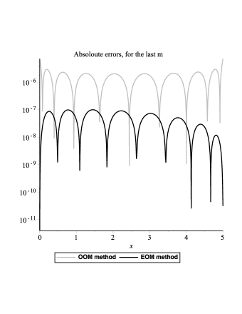
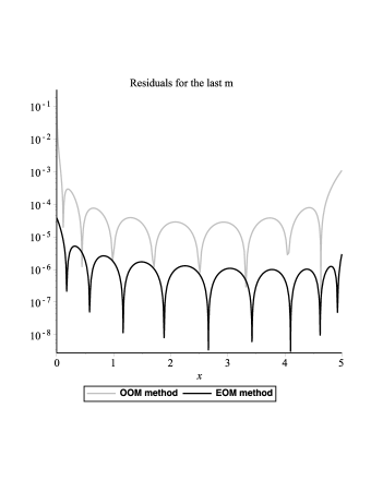
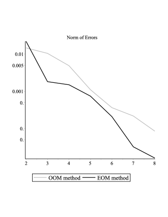
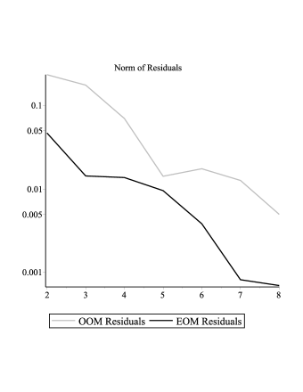
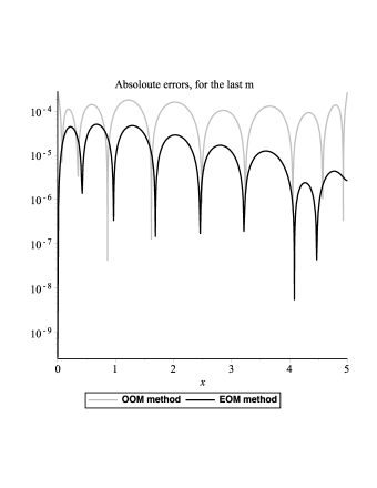
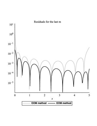
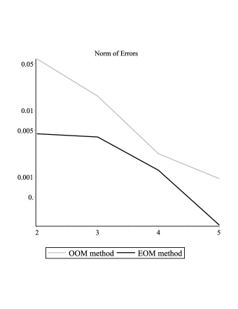
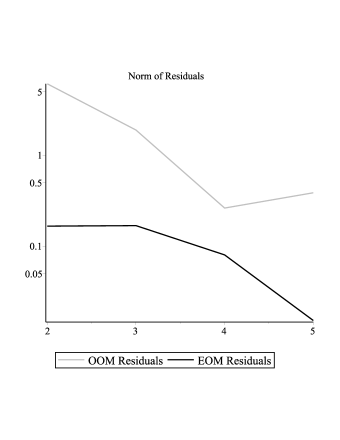
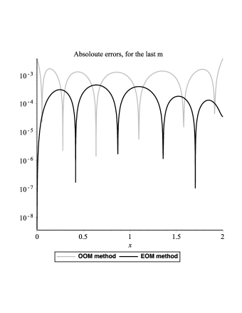
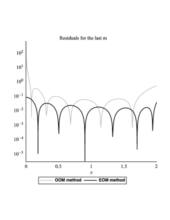
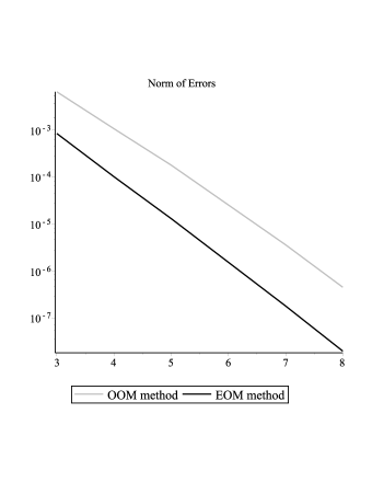
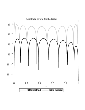
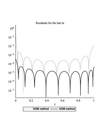
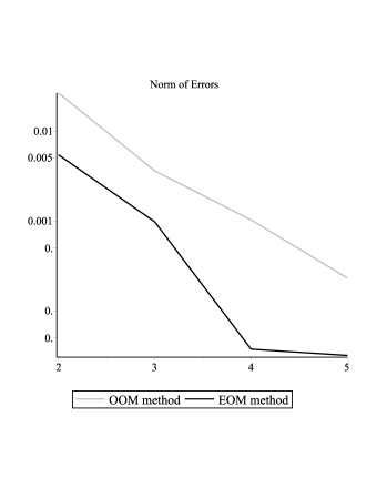
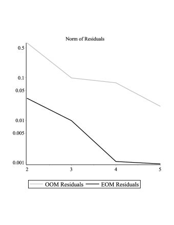
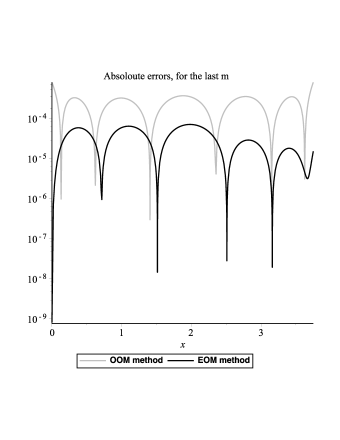
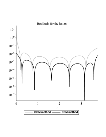
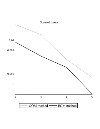
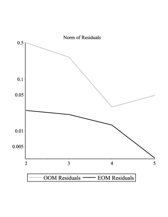
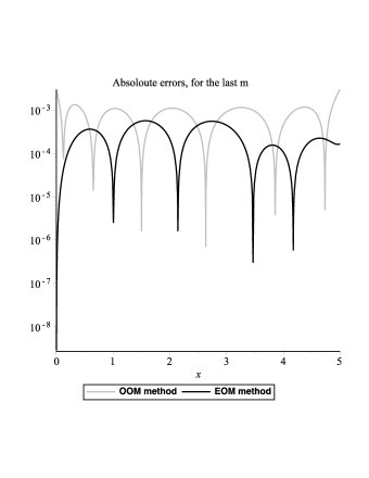
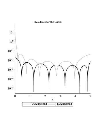
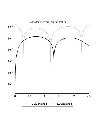
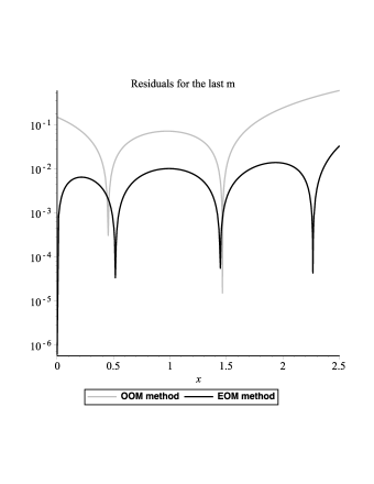
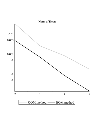
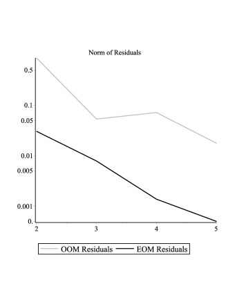
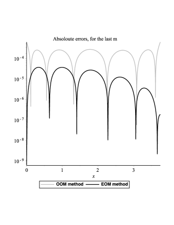
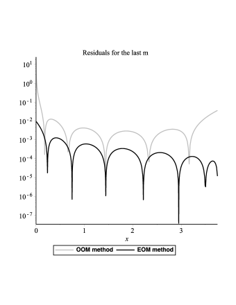
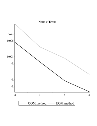
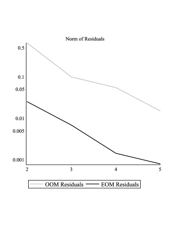
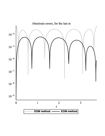
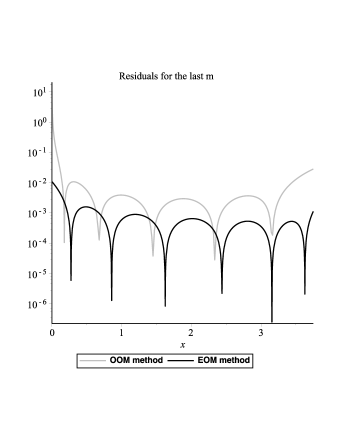
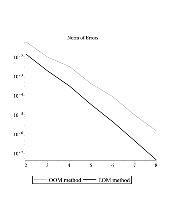
Where, E is the largest m𝑚m for which the results are reported. To evaluate the solution accuracy for each m𝑚m, it is not needed to check them one by one; reporting the norm of the residual and the error functions is enough for evaluation; so, we present two categories of figures. The first category contains the figures which report the norm of the residual or the error function, for all of the m𝑚m values, and the second category contains the plots of the error or the residual function for the largest m𝑚m value (E𝐸E),
Looking at the first category plots, we find out that both of the residual and the error function values decreases by increasing the m𝑚m value which confirms the convergence of both methods. Also, they demonstrate the absolute priority of EOM. the second category of plots shows that almost for all x𝑥x values, both of the residual and the error functions values of the EOM method are less than OOM. Meanwhile, the second category plots are semi-logarithmic, because, according to the high superiority of EOMs to OOMs, the error of the EOM method results can not be seen obviously, in non-logarithmic plots.
To have a good approximation of g(y(x))𝑔𝑦𝑥g(y(x)), we have used some large N𝑁N values like 8, 10, 12 and 15. The acceptable results accuracy shows the efficient choices for N𝑁N.
Before explaining the figures one by one, we should remind that the problem is solved in the interval x[0,M]𝑥0𝑀x\in[0,M]. The question is what value we should choose for M𝑀M? Like the previous researches, we are only interested in the positive y(x)𝑦𝑥y(x) values (we only solve the problems with positive y(0)𝑦0y(0) values). Remember that we have the (almost) exact solutions for all of the problems. Accordingly, we chose the M𝑀M as the point at which y(M)=0𝑦𝑀0y(M)=0. But if M>5𝑀5M>5, then we set M=5𝑀5M=5.
Here, we explain the plots one by one. The analytical solution of the equation (11) for y0(x)superscript𝑦0𝑥y^{0}(x) is so that we can exactly write it as a linear combination of the Bernstein polynomials; so, we do not report its figures. But, reports of the problem for y1(x)superscript𝑦1𝑥y^{1}(x) and y5(x)superscript𝑦5𝑥y^{5}(x) are depicted in the figures 1,2,3,4. The figures 5,6 show less accuracy than other problems. This shows that N𝑁N value is not sufficiently large to approximate g(y(x))𝑔𝑦𝑥g(y(x)), well. However, these kinds of results are appropriate to show the truncated series performance in function approximation. In the figures 7,8, which contains the (17) problem results, the analytical solution is compared with both methods approximate solutions and, obviously, shows the preference of the EOMs to OOMs, as for the previous problems. The problem (12) is solved twice, one time for g(y(x))=y32(x)𝑔𝑦𝑥superscript𝑦32𝑥g(y(x))=y^{\frac{3}{2}}(x) and the second time for g(y(x))=y52(x)𝑔𝑦𝑥superscript𝑦52𝑥g(y(x))=y^{\frac{5}{2}}(x) and the results are depicted in the figures 9,10,11,12. The figures 10 and 12 shows the ineligible results for the OOM method residual function. For example, in x=0𝑥0x=0, the error is even more than 1, while, even in those points, the EOM method presents some suitable results. The interesting point in the solution of the problem (13) for m=2𝑚2m=2, which is observable in the figure 13, is the ability to reach such high accuracy approximations, even for such a small m𝑚m, by choosing a large-enough value for N𝑁N, which in this problem is 15. The figures 14,15,16,17 as solution figures of the problems (14) and (15) again, show some almost ineligible results for OOM method, while EOMs have some suitable results.
Refer to caption
(a) Error(ym(x))1subscriptdelimited-∥∥𝐸𝑟𝑟𝑜𝑟subscript𝑦𝑚𝑥1\lVert Error\left(y_{m}(x)\right)\rVert_{1}
Refer to caption
(b) Residual(ym(x))1subscriptdelimited-∥∥𝑅𝑒𝑠𝑖𝑑𝑢𝑎𝑙subscript𝑦𝑚𝑥1\lVert Residual\left(y_{m}(x)\right)\rVert_{1}
Figure 1: the norm1 of the residual and error function plots for several m𝑚m values and f(x)=1,g(x)=y(x),N=8formulae-sequence𝑓𝑥1formulae-sequence𝑔𝑥𝑦𝑥𝑁8f(x)=1,~{}g(x)=y(x),~{}N=8
Refer to caption
(a) Error(yM(x))1subscriptdelimited-∥∥𝐸𝑟𝑟𝑜𝑟subscript𝑦𝑀𝑥1\lVert Error\left(y_{M}(x)\right)\rVert_{1}
Refer to caption
(b) Residual(yM(x))1subscriptdelimited-∥∥𝑅𝑒𝑠𝑖𝑑𝑢𝑎𝑙subscript𝑦𝑀𝑥1\lVert Residual\left(y_{M}(x)\right)\rVert_{1}
Figure 2: the norm1 of the residual and error function plots for the largest m𝑚m value (E𝐸E) of the figure (1) for f(x)=1,g(x)=y(x),N=8formulae-sequence𝑓𝑥1formulae-sequence𝑔𝑥𝑦𝑥𝑁8f(x)=1,~{}g(x)=y(x),~{}N=8
Refer to caption
(a) Error(ym(x))1subscriptdelimited-∥∥𝐸𝑟𝑟𝑜𝑟subscript𝑦𝑚𝑥1\lVert Error\left(y_{m}(x)\right)\rVert_{1}
Refer to caption
(b) Residual(ym(x))1subscriptdelimited-∥∥𝑅𝑒𝑠𝑖𝑑𝑢𝑎𝑙subscript𝑦𝑚𝑥1\lVert Residual\left(y_{m}(x)\right)\rVert_{1}
Figure 3: the norm1 of the residual and error function plots for several m𝑚m values and f(x)=1,g(x)=y5(x),N=8formulae-sequence𝑓𝑥1formulae-sequence𝑔𝑥superscript𝑦5𝑥𝑁8f(x)=1,~{}g(x)=y^{5}(x),~{}N=8
Refer to caption
(a) Error(yM(x))1subscriptdelimited-∥∥𝐸𝑟𝑟𝑜𝑟subscript𝑦𝑀𝑥1\lVert Error\left(y_{M}(x)\right)\rVert_{1}
Refer to caption
(b) Residual(yM(x))1subscriptdelimited-∥∥𝑅𝑒𝑠𝑖𝑑𝑢𝑎𝑙subscript𝑦𝑀𝑥1\lVert Residual\left(y_{M}(x)\right)\rVert_{1}
Figure 4: the norm1 of the residual and error function plots for the largest m𝑚m value (E𝐸E) of the figure (3) for f(x)=1,g(x)=y5(x),N=8formulae-sequence𝑓𝑥1formulae-sequence𝑔𝑥superscript𝑦5𝑥𝑁8f(x)=1,~{}g(x)=y^{5}(x),~{}N=8
Refer to caption
(a) Error(ym(x))1subscriptdelimited-∥∥𝐸𝑟𝑟𝑜𝑟subscript𝑦𝑚𝑥1\lVert Error\left(y_{m}(x)\right)\rVert_{1}
Refer to caption
(b) Residual(ym(x))1subscriptdelimited-∥∥𝑅𝑒𝑠𝑖𝑑𝑢𝑎𝑙subscript𝑦𝑚𝑥1\lVert Residual\left(y_{m}(x)\right)\rVert_{1}
Figure 5: the norm1 of the residual and error function plots for several m𝑚m values a f(x)=1,g(x)=4(2ey(x)+ey(x)2),N=10formulae-sequence𝑓𝑥1formulae-sequence𝑔𝑥42superscript𝑒𝑦𝑥superscript𝑒𝑦𝑥2𝑁10f(x)=1,~{}g(x)=4\left(2e^{y(x)}+e^{\frac{y(x)}{2}}\right),~{}N=10
Refer to caption
(a) Error(yM(x))1subscriptdelimited-∥∥𝐸𝑟𝑟𝑜𝑟subscript𝑦𝑀𝑥1\lVert Error\left(y_{M}(x)\right)\rVert_{1}
Refer to caption
(b) Residual(yM(x))1subscriptdelimited-∥∥𝑅𝑒𝑠𝑖𝑑𝑢𝑎𝑙subscript𝑦𝑀𝑥1\lVert Residual\left(y_{M}(x)\right)\rVert_{1}
Figure 6: the norm1 of the residual and error function plots for the largest m𝑚m value (E𝐸E) of the figure (5) for f(x)=1,g(x)=4(2ey(x)+ey(x)2,N=10)formulae-sequence𝑓𝑥1𝑔𝑥42superscript𝑒𝑦𝑥superscript𝑒𝑦𝑥2𝑁10f(x)=1,~{}g(x)=4\left(2e^{y(x)}+e^{\frac{y(x)}{2}},~{}N=10\right)
Refer to caption
(a) Error(ym(x))1subscriptdelimited-∥∥𝐸𝑟𝑟𝑜𝑟subscript𝑦𝑚𝑥1\lVert Error\left(y_{m}(x)\right)\rVert_{1}
Refer to caption
(b) Residual(ym(x))1subscriptdelimited-∥∥𝑅𝑒𝑠𝑖𝑑𝑢𝑎𝑙subscript𝑦𝑚𝑥1\lVert Residual\left(y_{m}(x)\right)\rVert_{1}
Figure 7: the norm1 of the residual and error function plots for several m𝑚m values and f(x)=2(2x2+3),g(x)=y(x),N=8formulae-sequence𝑓𝑥22superscript𝑥23formulae-sequence𝑔𝑥𝑦𝑥𝑁8f(x)=-2\left(2x^{2}+3\right),~{}g(x)=y(x),~{}N=8
Refer to caption
(a) Error(yM(x))1subscriptdelimited-∥∥𝐸𝑟𝑟𝑜𝑟subscript𝑦𝑀𝑥1\lVert Error\left(y_{M}(x)\right)\rVert_{1}
Refer to caption
(b) Residual(yM(x))1subscriptdelimited-∥∥𝑅𝑒𝑠𝑖𝑑𝑢𝑎𝑙subscript𝑦𝑀𝑥1\lVert Residual\left(y_{M}(x)\right)\rVert_{1}
Figure 8: the norm1 of the residual and error function plots for the largest m𝑚m value (E𝐸E) of the figure (7) for f(x)=2(2x2+3),g(x)=y(x),N=8formulae-sequence𝑓𝑥22superscript𝑥23formulae-sequence𝑔𝑥𝑦𝑥𝑁8f(x)=-2\left(2x^{2}+3\right),~{}g(x)=y(x),~{}N=8
Refer to caption
(a) Error(ym(x))1subscriptdelimited-∥∥𝐸𝑟𝑟𝑜𝑟subscript𝑦𝑚𝑥1\lVert Error\left(y_{m}(x)\right)\rVert_{1}
Refer to caption
(b) Residual(ym(x))1subscriptdelimited-∥∥𝑅𝑒𝑠𝑖𝑑𝑢𝑎𝑙subscript𝑦𝑚𝑥1\lVert Residual\left(y_{m}(x)\right)\rVert_{1}
Figure 9: the norm1 of the residual and error function plots for several m𝑚m values and f(x)=1,g(x)=y32(x),N=12formulae-sequence𝑓𝑥1formulae-sequence𝑔𝑥superscript𝑦32𝑥𝑁12f(x)=1,~{}g(x)=y^{\frac{3}{2}}(x),~{}N=12
Refer to caption
(a) Error(yM(x))1subscriptdelimited-∥∥𝐸𝑟𝑟𝑜𝑟subscript𝑦𝑀𝑥1\lVert Error\left(y_{M}(x)\right)\rVert_{1}
Refer to caption
(b) Residual(yM(x))1subscriptdelimited-∥∥𝑅𝑒𝑠𝑖𝑑𝑢𝑎𝑙subscript𝑦𝑀𝑥1\lVert Residual\left(y_{M}(x)\right)\rVert_{1}
Figure 10: the norm1 of the residual and error function plots for the largest m𝑚m value (E𝐸E) of the figure (9) for f(x)=1,g(x)=y32(x),N=12formulae-sequence𝑓𝑥1formulae-sequence𝑔𝑥superscript𝑦32𝑥𝑁12f(x)=1,~{}g(x)=y^{\frac{3}{2}}(x),~{}N=12
Refer to caption
(a) Error(ym(x))1subscriptdelimited-∥∥𝐸𝑟𝑟𝑜𝑟subscript𝑦𝑚𝑥1\lVert Error\left(y_{m}(x)\right)\rVert_{1}
Refer to caption
(b) Residual(ym(x))1subscriptdelimited-∥∥𝑅𝑒𝑠𝑖𝑑𝑢𝑎𝑙subscript𝑦𝑚𝑥1\lVert Residual\left(y_{m}(x)\right)\rVert_{1}
Figure 11: the norm1 of the residual and error function plots for several m𝑚m values and f(x)=1,g(x)=y52(x),N=12formulae-sequence𝑓𝑥1formulae-sequence𝑔𝑥superscript𝑦52𝑥𝑁12f(x)=1,~{}g(x)=y^{\frac{5}{2}}(x),~{}N=12
Refer to caption
(a) Error(yM(x))1subscriptdelimited-∥∥𝐸𝑟𝑟𝑜𝑟subscript𝑦𝑀𝑥1\lVert Error\left(y_{M}(x)\right)\rVert_{1}
Refer to caption
(b) Residual(yM(x))1subscriptdelimited-∥∥𝑅𝑒𝑠𝑖𝑑𝑢𝑎𝑙subscript𝑦𝑀𝑥1\lVert Residual\left(y_{M}(x)\right)\rVert_{1}
Figure 12: the norm1 of the residual and error function plots for the largest m𝑚m value (E𝐸E) of the figure (11) for f(x)=1,g(x)=y52(x),N=12formulae-sequence𝑓𝑥1formulae-sequence𝑔𝑥superscript𝑦52𝑥𝑁12f(x)=1,~{}g(x)=y^{\frac{5}{2}}(x),~{}N=12
Refer to caption
(a) Error(yM(x))1subscriptdelimited-∥∥𝐸𝑟𝑟𝑜𝑟subscript𝑦𝑀𝑥1\lVert Error\left(y_{M}(x)\right)\rVert_{1}
Refer to caption
(b) Residual(yM(x))1subscriptdelimited-∥∥𝑅𝑒𝑠𝑖𝑑𝑢𝑎𝑙subscript𝑦𝑀𝑥1\lVert Residual\left(y_{M}(x)\right)\rVert_{1}
Figure 13: the norm1 of the residual and error function for M=2𝑀2M=2 and f(x)=1,g(x)=ey(x),N=15formulae-sequence𝑓𝑥1formulae-sequence𝑔𝑥superscript𝑒𝑦𝑥𝑁15f(x)=1,~{}g(x)=e^{y(x)},~{}N=15
Refer to caption
(a) Error(ym(x))1subscriptdelimited-∥∥𝐸𝑟𝑟𝑜𝑟subscript𝑦𝑚𝑥1\lVert Error\left(y_{m}(x)\right)\rVert_{1}
Refer to caption
(b) Residual(ym(x))1subscriptdelimited-∥∥𝑅𝑒𝑠𝑖𝑑𝑢𝑎𝑙subscript𝑦𝑚𝑥1\lVert Residual\left(y_{m}(x)\right)\rVert_{1}
Figure 14: the norm1 of the residual and error function plots for several m𝑚m values and f(x)=1,g(x)=sinh(y(x)),N=10formulae-sequence𝑓𝑥1formulae-sequence𝑔𝑥𝑦𝑥𝑁10f(x)=1,~{}g(x)=\sinh(y(x)),~{}N=10
Refer to caption
(a) Error(yM(x))1subscriptdelimited-∥∥𝐸𝑟𝑟𝑜𝑟subscript𝑦𝑀𝑥1\lVert Error\left(y_{M}(x)\right)\rVert_{1}
Refer to caption
(b) Residual(yM(x))1subscriptdelimited-∥∥𝑅𝑒𝑠𝑖𝑑𝑢𝑎𝑙subscript𝑦𝑀𝑥1\lVert Residual\left(y_{M}(x)\right)\rVert_{1}
Figure 15: the norm1 of the residual and error function plots for the largest m𝑚m value (E𝐸E) of the figure (14) for f(x)=1,g(x)=sinh(y(x)),N=10formulae-sequence𝑓𝑥1formulae-sequence𝑔𝑥𝑦𝑥𝑁10f(x)=1,~{}g(x)=\sinh(y(x)),~{}N=10
Refer to caption
(a) Error(ym(x))1subscriptdelimited-∥∥𝐸𝑟𝑟𝑜𝑟subscript𝑦𝑚𝑥1\lVert Error\left(y_{m}(x)\right)\rVert_{1}
Refer to caption
(b) Residual(ym(x))1subscriptdelimited-∥∥𝑅𝑒𝑠𝑖𝑑𝑢𝑎𝑙subscript𝑦𝑚𝑥1\lVert Residual\left(y_{m}(x)\right)\rVert_{1}
Figure 16: the norm1 of the residual and error function plots for several m𝑚m values and f(x)=1,g(x)=sin(y(x)),N=12formulae-sequence𝑓𝑥1formulae-sequence𝑔𝑥𝑦𝑥𝑁12f(x)=1,~{}g(x)=\sin(y(x)),~{}N=12
Refer to caption
(a) Error(yM(x))1subscriptdelimited-∥∥𝐸𝑟𝑟𝑜𝑟subscript𝑦𝑀𝑥1\lVert Error\left(y_{M}(x)\right)\rVert_{1}
Refer to caption
(b) Residual(yM(x))1subscriptdelimited-∥∥𝑅𝑒𝑠𝑖𝑑𝑢𝑎𝑙subscript𝑦𝑀𝑥1\lVert Residual\left(y_{M}(x)\right)\rVert_{1}
Figure 17: the norm1 of the residual and error function plots for the largest m𝑚m value (E𝐸E) of the figure (16) for f(x)=1,g(x)=sin(y(x)),N=12formulae-sequence𝑓𝑥1formulae-sequence𝑔𝑥𝑦𝑥𝑁12f(x)=1,~{}g(x)=\sin(y(x)),~{}N=12

5 Concluding Remarks and suggestions for further study

In this paper, we implemented the recently introduced exact operational matrices (EOMs) [20] of the Bernstein polynomials to solve the well-known Emden-Fowler equations. To do so, well, it was necessary to achieve a relation for the best coefficients eisubscript𝑒𝑖e_{i} to approximate a function g(x)𝑔𝑥g(x) in the form of i=1Neixisuperscriptsubscript𝑖1𝑁subscript𝑒𝑖superscript𝑥𝑖\sum_{i=1}^{N}{e_{i}x^{i}}. Then, we introduced a new matrix named by ”series operational matrix” for finding the coefficients sisubscript𝑠𝑖s_{i} to write the function g(y(x))𝑔𝑦𝑥g\left(y(x)\right) in the form of i=0mNsiBi,mN(x)superscriptsubscript𝑖0𝑚𝑁subscript𝑠𝑖subscript𝐵𝑖𝑚𝑁𝑥\sum_{i=0}^{m\cdot N}{s_{i}B_{i,m\cdot N}(x)} where Bi,mN(x)subscript𝐵𝑖𝑚𝑁𝑥B_{i,m\cdot N}(x)s are the Bernstein polynomials of degree mN𝑚𝑁m\cdot N.
The differential equations which EOM idea were applied to solve them, are either linear or low-order nonlinear problems; so, the reported results [20] were not comprehensive criteria for the superiority of the new method; therefore, we chose Emden-Fowler type equations, which have a high-order nonlinearity (because of the presence of the g(y(x))i=0mNeiBi,mN(x)similar-to-or-equals𝑔𝑦𝑥superscriptsubscript𝑖0𝑚𝑁subscript𝑒𝑖subscript𝐵𝑖𝑚𝑁𝑥g\left(y(x)\right)\simeq\sum_{i=0}^{m\cdot N}{e_{i}B_{i,m\cdot N}(x)} approximation), to be solved by EOMs.
For solving the differential equations by the Galerkin method, using the EOMs, we reached an almost exact residual function (Residual(x)𝑅𝑒𝑠𝑖𝑑𝑢𝑎𝑙𝑥Residual(x)) which was never obtainable by the old ”ordinary operational matrices” (OOMs) in most of the problems. We converted the residual function to a system of algebraic equations using the Galerkin operational matrix [20] and solved them to find the unknown function y(x)𝑦𝑥y(x).
To have an appropriate criterion for the results accuracy of those problems which does not have exact solution, we solved the problem using a seventh-eighth order continuous Runge-Kutta method as an almost exact solution, using the Maple© dverk78 function.
To see the results error convergence to zero, we applied the Galerkin method repeatedly, each new step with a larger ψn(x)subscript𝜓𝑛𝑥\psi_{n}(x). Then, we reported the decreasing norm of errors in some plots. The reported results show the superiority of EOMs over OOMs. Using the (almost) exact solution, we reported the norm1 of both methods error. We did the same for both residual functions. Then, we compared these result pairs, reporting their proportions.
The Emden-Fowler problem domain is [0,)0[0,\infty); for solving it by the Bernstein polynomials which are defined on the domain [0,1]01[0,1], firstly, we truncated the problem domain to [0,M]0𝑀[0,M] and then used a mapping to change its variable and solved it.
As some future works, EOM idea can be implemented for other basis functions. Also, solving differential equations which have much close solutions to the vector space made by the Bernstein polynomials and some determinate norm, can illustrate the EOM efficiency much clear.

References

  • [1] B. G. Galerkin, Sterzhni i plastinki: Riady v nekotorykh voprosakh uprugogo ravnovesiia sterzhnei i plastinok, Vestnik inzhenerov. 1 (1915) 897–908.
  • [2] W. Ritz, Über eine neue methode zur lösung gewisser variationsprobleme der mathematischen physik, Journal für die reine und angewandte Mathematik 135.
  • [3] A. M. Prokhorov, The Great Soviet Encyclopedia, 3rd Edition, Collier Macmillan Publishers, London, 1973.
  • [4] C. F. Chen, C. H. Hsiao, A state-space approach to Walsh series solution of linear systems, Int. J. Syst. Sci. 122 (1975) 565–570.
  • [5] C. F. Chen, Y. T. Tsay, T. T. Wu, Walsh operational matrices for fractional calculus and their application to distributed system, J. of Franklin Institute 303 (1977) 267–284.
  • [6] S.G.Mouroutsos, P. Sparis, Taylor series approach to system identification, analysis and optimal control, J. Franklin I. 325 (1988) 359–371.
  • [7] M. Razzaghi, M. Razzaghi, Fourier series direct method for variational problems, I. J. Control 48 (1988) 887–895.
  • [8] M. Razzaghi, M. Razzaghi, Taylor series analysis of time-varying multi-delay systems, I. J. Control 50 (1989) 183–192.
  • [9] M. Razzaghi, M. Razzaghi, Shifted-Jacobi series direct method for variational problems, Int. J. Syst. Sci. 20 (1989) 1119–1129.
  • [10] W. Bolek, Derivation of operational matrices of differentiation for orthogonal polynomials, Automatica 29 (1993) 1607–1609.
  • [11] M. Razzaghi, S. Yousefi, Legendre wavelets direct method for variational problems, Math. Comput. Simulat. 53 (2000) 185–192.
  • [12] H. Jafari, S. Yousefi, M. Firoozjaee, S. Momani, C. Khaliqued, Application of Legendre wavelets for solving fractional differential equations, Comput. Math. Appl. 62 (2011) 1038–1045.
  • [13] F. Khellat, S. Yousefi, The linear Legendre mother wavelets operational matrix of integration and its application, J. Franklin I. 343 (2006) 181–190.
  • [14] S. Yousefi, M. Behroozifar, M. Dehghan, Numerical solution of the nonlinear age-structured population models by using the operational matrices of Bernstein polynomials, Appl. Math. Modell. 36 (2012) 945–963.
  • [15] S. Yousefi, M. Behroozifar, M. Dehghan, The operational matrices of Bernstein polynomials for solving the parabolic equation subject to specification of the mass, J. Comput. Appl. Math. 335 (2011) 5272–5283.
  • [16] S. A. Yousefi, M. Behroozifar, Operational matrices of Bernstein polynomials and their applications, I. J. Sys. Sci. 41 (2010) 709–716.
  • [17] S. Kazem, M. Shaban, J. A. Rad, Solution of the coupled burgers equation based on operational matrices of d-dimensional orthogonal functions, Z. Naturforsch. A 67 (2012) 267–274.
  • [18] M. Shaban, S. Kazem, J. A. Rad, A modification of the homotopy analysis method based on Chebyshev operational matrices, Math. Comput. Model. (2013), in press.
  • [19] S. Kazem, An integral operational matrix based on Jacobi polynomials for solving fractional-order differential equations, Appl. Math. Modell. 37 (2013) 1126–1136.
  • [20] K. Parand, S. A. Kaviani, Application of the exact operational matrices based on the Bernstein polynomials, J. Math. comput. sci. 6 (2013) 36–59.
  • [21] S. Chandrasekhar, Introduction to the Study of Stellar Structure, Dover, 1967.
  • [22] H. T. Davis, Introduction to Nonlinear Differential and Integral Equations, Dover, 1962.
  • [23] O. U. Richardson, The Emission of Electricity from Hot Bodies, Longman’s Green and Company, 1921.
  • [24] A. Aslanov, Determination of convergence intervals of the series solutions of Emden-Fowler equations using polytropes and isothermal spheres, Phys. Lett. A 372 (2008) 3555–3561.
  • [25] R. P. Agarwal, D. O’Regan, Second order initial value problems of Lane-Emden type, Appl. Math. Lett. 20 (2007) 1198–1205.
  • [26] C. M. Bender, K. A. Milton, S. S. Pinsky, L. M. S. Jr., A new perturbative approach to nonlinear problems, J. Math. Phys. 30 (1989) 1447–1455.
  • [27] N. T. Shawagfeh, Nonperturbative approximate solution for Lane-Emden equation, J. Math. Phys. 34 (1993) 4364–4369.
  • [28] V. B. Mandelzweig, F. Tabakin, Quasilinearization approach to nonlinear problems in physics with application to nonlinear ODEs, Comput. Phys. Commun. 141 (2001) 268–281.
  • [29] A. M. Wazwaz, A new algorithm for solving differential equations of Lane-Emden type, Appl. Math. Comput. 118 (2001) 287–310.
  • [30] A. M. Wazwaz, The modified decomposition method for analytic treatment of differential equations, Appl. Math. Comput. 173 (2006) 165–176.
  • [31] S. Liao, A new analytic algorithm of Lane-Emden type equations, Appl. Math. Comput. 142 (2003) 1–16.
  • [32] J. H. He, Variational approach to the Lane-Emden equation, Appl. Math. Comput. 143 (2003) 539–541.
  • [33] K. Parand, M. Razzaghi, Rational Legendre approximation for solving some physical problems on semi-infinite intervals, Phys. Scr. 69 (2004) 353–357.
  • [34] J. I. Ramos, Linearization techniques for singular initial-value problems of ordinary differential equations, Appl. Math. Comput. 161 (2005) 525–542.
  • [35] J. I. Ramos, Piecewise-adaptive decomposition methods, Chaos Soliton Fract. 40 (2009) 1623–1636.
  • [36] J. I. Ramos, Series approach to the Lane-Emden equation and comparison with the homotopy perturbation method, Chaos Soliton Fract. 38 (2008) 400–408.
  • [37] S. Yousefi, Legendre wavelets method for solving differential equations of Lane-Emden type, Appl. Math. Comput. 181 (2006) 1417–1422.
  • [38] A. Aslanov, Determination of convergence intervals of the series solutions of Emden-Fowler equations using polytropes and isothermal spheres, Phys. Lett. A 372 (2008) 3555–3561.
  • [39] M. Dehghan, F. Shakeri, Approximate solution of a differential equation arising in astrophysics using the variational iteration method, New Astron. 13 (2008) 53–59.
  • [40] M. S. H. Chowdhury, I. Hashim, Solutions of Emden-Fowler equations by homotopy-perturbation method, Nonlinear Anal. Real 10 (2009) 104–115.
  • [41] A. S. Bataineh, M. S. M. Noorani, I. Hashim, Homotopy analysis method for singular IVPs of Emden-Fowler type, Commun. Nonlinear Sci. Numer. Simul. 14 (2009) 1121–1131.
  • [42] K. Parand, M. Shahini, M. Dehghan, Rational Legendre pseudospectral approach for solving nonlinear differential equations of Lane-Emden type, J. Comput. Phys. 228 (2009) 8830–8840.
  • [43] K. Parand, M. Dehghan, A. R. Rezaei, S. M. Ghaderi, An approximation algorithm for the solution of the nonlinear Lane-Emden type equations arising in astrophysics using Hermite functions collocation method, Computer Physics Communications 181 (2010) 1096–1108.
  • [44] K. Parand, S. Abbasbandy, S. Kazem, A. R. Rezaei, An improved numerical method for a class of astrophysics problems based on radial basis functions, Phys. Scr. 83 (2011) 015011.
  • [45] K. Parand, A. R. Rezaei, A. Taghavi, Lagrangian method for solving Lane-Emden type equation arising in astrophysics on semi-infinite domains, Acta Astoraut. 67 (2010) 673–680.
  • [46] K. Parand, A. Pirkhedri, Sinc-Collocation methode for solving astrophysics equations, New Astron. 15 (2010) 533–537.
  • [47] C. M. Khalique, P. Ntsime, Exact solutions of the Lane-Emden-type equation, New Astron. 13 (2008) 476–480.
  • [48] R. A. V. Gorder, An elegant perturbation solution for the Lane-Emden equation of the second kind, New Astron. 16 (2011) 65–67.
  • [49] R. A. V. Gorder, Exact first integrals for a Lane-Emden equation of the second kind modeling a thermal explosion in a rectangular slab, New Astron. 16 (2011) 492–497.
  • [50] R. K. Pandey, N. Kumar, Solution of Lane-Emden type equations using Bernstein operational matrix of differentiation, New Astron. 17 (2012) 303–308.
  • [51] K. Boubaker, R. A. V. Gorder, Application of the BPES to Lane-Emden equations governing polytropic and isothermal gas spheres, New Astron. 17 (2012) 565–569.
  • [52] E. W. Weisstein, CRC Concise Encyclopedia of Mathematics, 2nd Edition, Chapman and Hall/CRC, Champaign, Illinois, 2002.
  • [53] A. Chakrabarti, S. C. Martha, Approximate solutions of Fredholm integral equations of the second kind, Appl. Math. Comput. 211 (2009) 459–466.
  • [54] B. N. Mandal, S. Bhattacharya, Numerical solution of some classes of integral equations using Bernstein polynomials, Appl. Math. Comput. 190 (2007) 1707–1716.
  • [55] S. Bhattacharya, B. N. Mandal, Use of Bernstein polynomials in numerical solutions of Volterra integral equations, Appl. Math. Sci. 2 (2008) 1773–1787.
  • [56] K. Maleknejad, E. Hashemizadeh, B. Basirat, Computational method based on Bernestein operational matrices for nonlinear Volterra-Fredholm-Hammerstein integral equations, Commun. Nonl. Sci. Numer. Simul. 17 (2012) 52–61.
  • [57] A. K. Singh, V. K. Singh, O. P. Singh, The Bernstein operational matrix of integration, Appl. Math. Sci. 3 (2009) 2427–2436.
  • [58] D. D. Bhatta, M. I. Bhatti, Numerical solution of KdV equation using modified Bernstein polynomials, Appl. Math. Comput. 174 (2006) 1255–1268.
  • [59] M. I. Bhatti, P. Bracken, Solutions of differential equations in a Bernstein polynomial basis, J. Comput. Appl. Math. 205 (2007) 272–280.
  • [60] S. Bhattacharya, B. N. Mandal, Numerical solution of a singular integro-differential equation, Appl. Math. Comput. 195 (2008) 346–350.
  • [61] S. Yousefi, M. Behroozifar, M. Dehghan, The operational matrices of Bernstein polynomials for solving the parabolic equation subject to specification of the mass, J. Comput. Appl. Math. 335 (2011) 5272–5283.