We initiate the study of relaxation to quantum equilibrium over long timescales in pilot-wave theory. We simulate the time evolution of the coarse-grained $H$-function $\bar{H}(t)$ for a two-dimensional harmonic oscillator. For a (periodic) wave function that is a superposition of the first 25 energy states we confirm an approximately exponential decay of $\bar{H}$ over five periods. For a superposition of only the first four energy states we are able to calculate $\bar{H}(t)$ over 50 periods. We find that, depending on the set of phases in the initial wave function, $\bar{H}$ can decay to a large nonequilibrium residue exceeding $10\%$ of its initial value or it can become indistinguishable from zero (the equilibrium value). We show that a large residue in $\bar{H}$ is caused by a tendency for the trajectories to be confined to sub-regions of configuration space for some wave functions, and that this is less likely to occur for larger numbers of energy states (if the initial phases are chosen randomly). Possible cosmological implications are briefly discussed.

1 Introduction

In the de Broglie-Bohm pilot-wave formulation of quantum theory [1, 2, 3, 4, 5], a system has an actual configuration $q(t)$ which evolves in time with a velocity $\dot{q}\equiv dq/dt$ that is determined by the wave function $\psi(q,t)$, where $\psi$ satisfies the Schrödinger equation $i\partial\psi/\partial t=\hat{H}\psi$ (taking $\hbar=1$). For standard Hamiltonians, $\dot{q}$ is proportional to the gradient $\partial_{q}S$ of the phase $S$ of $\psi$. Generally, $\dot{q}=j/|\psi|^{2}$ where $j=j\left[\psi\right]=j(q,t)$ is the Schrödinger current [6]. Here $\psi$ is a ‘pilot wave’ in configuration space that guides the motion of an individual system; it has no a priori connection with probabilities.

For an ensemble of systems with the same initial wave function $\psi(q,t_{i})$, we may consider an arbitrary initial distribution $\rho(q,t_{i})$ of configurations $q(t_{i})$. The time evolution $\rho(q,t)$ of the distribution will be determined by the continuity equation

$$\frac{\partial\rho}{\partial t}+\partial_{q}\cdot\left(\rho\dot{q}\right)=0\ .$$ (1)

Because $\left|\psi\right|^{2}$ obeys the same continuity equation, an initial distribution $\rho(q,t_{i})=\left|\psi(q,t_{i})\right|^{2}$ will evolve into $\rho(q,t)=\left|\psi(q,t)\right|^{2}$. In this state of ‘quantum equilibrium’ the probability distribution matches the Born rule. But in pilot-wave theory one may just as well consider ‘nonequilibrium’ distributions $\rho(q,t_{i})\neq\left|\psi(q,t_{i})\right|^{2}$ (just as in classical mechanics one may consider non-thermal distributions) [7, 8, 9].

As is well known, pilot-wave dynamics reproduces the empirical predictions of quantum theory if the initial ensemble is in quantum equilibrium ($\rho(q,t_{i})=\left|\psi(q,t_{i})\right|^{2}$) [3, 4]. However, for an initial nonequilibrium ensemble ($\rho(q,t_{i})\neq\left|\psi(q,t_{i})\right|^{2}$), the statistical predictions will generally disagree with quantum theory. Quantum physics may then be regarded as a special equilibrium case of a wider nonequilibrium physics [7, 8, 9, 10, 11, 12, 13, 14, 15, 16, 17].

The quantum-theoretical equilibrium state $\rho_{\mathrm{QT}}=\left|\psi\right|^{2}$ may be seen to arise from a process of relaxation analogous to classical thermal relaxation. The approach to equilibrium may be quantified by the coarse-grained $H$-function

$$\bar{H}=\int dq\ \bar{\rho}\ln(\bar{\rho}/\bar{\rho}_{\mathrm{QT}})\ ,$$ (2)

where $\bar{\rho}$, $\bar{\rho}_{\mathrm{QT}}$ are respectively obtained by averaging $\rho$, $\rho_{\mathrm{QT}}$ over (non-overlapping) coarse-graining cells. This function obeys a coarse-graining $H$-theorem $\bar{H}(t)\leq\bar{H}(0)$ (assuming that the initial state at $t=0$ has no fine-grained micro-structure), where the minimum $\bar{H}=0$ corresponds to equilibrium $\bar{\rho}=\bar{\rho}_{\mathrm{QT}}$ [7, 9, 11]. Like the analogous classical result, this theorem provides a general mechanism in terms of which one can understand how equilibrium is approached, while not proving that equilibrium is actually reached. The extent to which relaxation occurs will depend on the system and on the initial conditions. Extensive numerical simulations have been performed for initial wave functions that are superpositions of energy eigenstates. It has been found that initial nonequilibrium distributions $\rho$ rapidly approach $\rho_{\mathrm{QT}}$ on a coarse-grained level (that is, $\bar{\rho}\longrightarrow\bar{\rho}_{\mathrm{QT}}$) [9, 11, 18, 19, 20], with an approximately exponential decay of $\bar{H}(t)$ with time [18, 19].

The rapid relaxation seen in these simulations suggests that we may understand the Born rule as having arisen from a relaxation process that presumably took place in the remote past. Quantum nonequilibrium may have existed in the early universe, at very early times before relaxation took place [7, 8, 9, 10]. This could have left observable traces today – in the cosmic microwave background (CMB) or in relic particles that decoupled at very early times [11, 13, 14, 15, 16, 21]. But for ordinary laboratory systems one may reasonably expect to find quantum equilibrium today to high accuracy (as has been experimentally confirmed in a wide range of conditions). This expectation rests on the assumption that over long timescales relaxation will continue until any residual nonequilibrium becomes very small [9]. Given the results of numerical simulations carried out so far, and given the extremely violent history of our universe, this assumption seems reasonable. Still, the assumption should be tested with more extensive simulations that aim at probing relaxation in the long-time limit. One of the purposes of this paper is to initiate such a study.

Another point that requires further study is the generality of the relaxation process. As in classical statistical mechanics, there will always be initial states that do not relax to equilibrium. For example, the ground state of a box or oscillator has vanishing de Broglie velocity ($\partial_{q}S=0$) so that any initial nonequilibrium distribution will be static and cannot relax. But to understand the quantum probabilities that we observe today, we must bear in mind that every system we have access to has a long and violent astrophysical history – during which its quantum state will have been a complicated superposition of many energy states. What matters is what realistically might have occurred in the remote past in our actual universe. Could there exist realistic early states that do not relax?

Contopoulos et al. [22] have shown that, for a two-dimensional oscillator in a superposition of three or four energy states, there are some choices of initial wave function for which relaxation is limited and may hardly occur at all (see also ref. [23]). In these cases the trajectories are confined to sub-regions of configuration space and do not explore the whole support of $\left|\psi\right|^{2}$. It was found that this can occur regardless of whether or not the trajectories are chaotic. In some of the examples studied the trajectories are excluded from a small sub-region so that relaxation does not occur completely; in other examples the trajectories are confined to a small sub-region so that there is hardly any relaxation. The behaviour of the trajectories depends on the initial wave function (which determines the velocity field); it also depends on the support of the initial distribution (which determines where the trajectories begin). A similar example was given by Colin [20] for a Dirac fermion in a spherical box: for certain superpositions of three energy states trajectories are trapped inside a ‘core’ close to the origin, so that initial distributions confined to the core do not relax. These examples raise the question of how common such confinement is, and whether states of the early universe are likely to exhibit such behaviour.

Inflationary cosmology opens an empirical window onto quantum probabilities in the very early universe. According to our best current understanding, the observed temperature anisotropy of the CMB was seeded by quantum fluctuations in a scalar field during an early period of inflationary expansion [24, 25, 26, 27]. It has been shown that quantum nonequilibrium during the inflationary phase could leave an observable imprint today in the CMB [13, 14, 16, 21]. Thus the possibility of quantum nonequilibrium in the early universe can be tested using inflationary cosmology.

It has also been shown that relaxation can be suppressed at long wavelengths on expanding space [13, 14, 16, 21, 28]. In a cosmology with a ‘pre-inflationary’ phase – for example a period of radiation-dominated expansion, prior to inflation [29, 30, 31, 32, 33] – one may then expect to find a large-scale power deficit in the CMB (above some critical wavelength) [13, 14, 16, 21]. Such a deficit has recently been found in data from the Planck satellite [34]. It is conceivable that the observed deficit is caused by relaxation suppression during a pre-inflationary era, though of course it might also be due to some other effect. (For a detailed discussion see refs. [16, 21].)

It may also be of interest to consider a cosmological pre-inflationary phase with a very small number of excitations above the vacuum, since during inflation itself it is generally assumed that the quantum state is in or very close to the vacuum. If the pre-inflationary phase contained a very small number of excitations, one would like to know whether or not equilibrium is to be expected at the onset of inflation itself (and hence whether to expect anomalies in the CMB). This motivates us to study relaxation for states containing a small number of energy states – another focus of the present paper.

It suffices to consider the two-dimensional harmonic oscillator, since this system arises in high-energy field theory and cosmology when one considers a decoupled (that is, unentangled) field mode. To see this, consider a free, minimally-coupled, and massless scalar field $\phi$ on an expanding flat space with scale factor $a(t)$ (where $t$ is standard cosmological time). Working in Fourier space, with field components $\phi_{\mathbf{k}}(t)$, physical wavelengths are proportional to $a(t)$. If we write $\phi_{\mathbf{k}}$ in terms of its real and imaginary parts, $\phi_{\mathbf{k}}=\frac{\sqrt{V}}{(2\pi)^{3/2}}\left(q_{\mathbf{k}1}+iq_{\mathbf{k}2}\right)$ (where $V$ is a normalisation volume), in terms of the real variables $q_{\mathbf{k}r}$ the field Hamiltonian becomes a sum $H=\sum_{\mathbf{k}r}H_{\mathbf{k}r}$, where $H_{\mathbf{k}r}$ is the Hamiltonian of a harmonic oscillator with mass $m=a^{3}$ and angular frequency $\omega=k/a$ [13, 14, 16]. An unentangled mode $\mathbf{k}$ has an independent dynamics, with wave function $\psi_{\mathbf{k}}(q_{\mathbf{k}1},q_{\mathbf{k}2},t)$. Dropping the index $\mathbf{k}$, the wave function $\psi=\psi(q_{1},q_{2},t)$ satisfies the Schrödinger equation

$$i\frac{\partial\psi}{\partial t}=\sum_{r=1,\ 2}\left(-\frac{1}{2m}\partial_{r}^{2}+\frac{1}{2}m\omega^{2}q_{r}^{2}\right)\psi\ ,$$ (3)

while de Broglie’s equation of motion for the configuration $(q_{1},q_{2})$ reads

$$\dot{q}_{r}=\frac{1}{m}\operatorname{Im}\frac{\partial_{r}\psi}{\psi}$$ (4)

(with $\partial_{r}\equiv\partial/\partial q_{r}$). The marginal distribution $\rho=\rho(q_{1},q_{2},t)$ for the mode evolves according to

$$\frac{\partial\rho}{\partial t}+\sum_{r=1,\ 2}\partial_{r}\left(\rho\frac{1}{m}\operatorname{Im}\frac{\partial_{r}\psi}{\psi}\right)=0\ .$$ (5)

Equations (3)–(5) are identical to those of pilot-wave dynamics for a nonrelativistic two-dimensional harmonic oscillator with a time-dependent mass $m=a^{3}$ and time-dependent angular frequency $\omega=k/a$. Thus we may discuss relaxation for a single field mode in terms of relaxation for a nonrelativistic harmonic oscillator [13, 14].

It has been shown that the time evolution defined by equations (3)–(5) is mathematically equivalent to the time evolution of a standard harmonic oscillator (with constant mass $m$ and constant angular frequency $\omega$) but with real time replaced by a ‘retarded time’ that depends on the wavelength of the mode [21]. This result shows that cosmological relaxation for a single field mode may be discussed in terms of relaxation for a standard harmonic oscillator. (In the short-wavelength limit the retarded time reduces to real time and we recover the time evolution of a field mode on Minkowski spacetime. In this limit, if the field mode is in a superposition of different states of definite occupation number, then relaxation will take place as for an ordinary oscillator. On the other hand, at long wavelengths – roughly speaking, for physical wavelengths larger than the Hubble radius $H^{-1}\equiv a/\dot{a}$ – relaxation is retarded. See ref. [21].)

In this paper we therefore study relaxation for the standard two-dimensional harmonic oscillator – in the long-time limit and also with a small number of excitations. We calculate as far ahead in time as we are able to guarantee accurate results. We pay particular attention to the accuracy of our calculations of $\bar{H}(t)$, with a view to quantifying the precise extent of relaxation in the long-time limit. We are especially interested in the following questions. For a given initial wave function, does $\bar{H}(t)$ continue to decrease approximately exponentially for an indefinite period of time or does the decay eventually halt? If there are only a tiny number of energy states in the superposition, can the resulting very slow evolution nevertheless eventually drive the system to equilibrium to high accuracy? To what extent does the behaviour of $\bar{H}(t)$ depend on the details of the initial quantum state?

We first consider (Section 3) a case where the wave function is a superposition of 25 energy states. The approximate exponential decay of $\bar{H}(t)$ is found to continue for as far in time as we are able to simulate reliably, with $\bar{H}(t)$ reaching a final value that is smaller than $1\%$ of its initial value. We then consider (Section 4) a case where the wave function is a superposition of four energy states. We find that $\bar{H}(t)$ decays approximately exponentially at first but eventually the decay halts and the function $\bar{H}(t)$ levels off to a roughly constant ‘residue’ that exceeds $10\%$ of the initial value. To explain the difference between these two cases, we consider (Section 5) the extent to which the trajectories explore the full support of $\left|\psi\right|^{2}$. For the first case we find negligible confinement to sub-regions, while for the second case we find strong confinement. Thus we may explain the large residue in $\bar{H}(t)$ for the second case as due to a lack of full exploration of the support of $\left|\psi\right|^{2}$ by the trajectories, along the lines found by Contopoulos et al. [22]. We also consider how common these different kinds of behaviour are likely to be. While a full answer is left to future research, we present evidence that confinement of trajectories – and an associated large residue in $\bar{H}$ – are less likely to occur when the initial wave function contains a larger number of superposed energy states. This suggests that a large nonequilibrium residue, as quantified by a large non-zero value of $\bar{H}$, is likely to be cosmologically relevant only in scenarios containing a very small number of energy states (for example, during pre-inflation).

Before proceeding let us summarise previous numerical work in which the time evolution of $\bar{H}$ was studied. For all the systems studied so far, including that in this paper, the wave function is periodic in time. In refs. [9, 11] numerical simulations were carried out for the artificial case of a one-dimensional box, for which relaxation can take place only to a very limited degree. For a wave function that is a superposition of the first 10 energy states, values of $\bar{H}(t)$ were obtained over just $1\%$ of a period, with an initial value $\simeq 0.61$ and a final value $\simeq 0.56$, so that $\bar{H}$ dropped only slightly – to about $90\%$ of its initial value. In ref. [18] simulations were carried out for a two-dimensional box with a superposition of the first 16 energy states. Values of $\bar{H}(t)$ were obtained over half a period, with an initial value $\simeq 0.74$ and a final value $\simeq 0.18$, so that $\bar{H}$ dropped to about $25\%$ of its initial value. In ref. [19] further simulations were carried out for the same system, for varying numbers of energy states superposed in the wave function. Values of $\bar{H}(t)$ were obtained over a whole period. For example, for $16$ energy states it was found that an initial value $\simeq 0.84$ decreased to $\simeq 0.08$ – that is, $\bar{H}$ dropped to about $10\%$ of its initial value. Finally, in ref. [21] simulations were carried out for the standard oscillator with a superposition of the first 25 energy states. (See the case of no spatial expansion, shown in figures 3 and 4 of ref. [21].) Values of $\bar{H}(t)$ were obtained over five periods, with an initial value $\simeq 1.27$ and a final value $\simeq 0.07$, so that $\bar{H}$ dropped to about $5\%$ of its initial value. In refs. [18, 19] an approximate exponential decay $\bar{H}(t)\approx\bar{H}(0)\exp(-t/\tau)$ was observed over the whole of the time intervals considered (where $\tau$ is the relaxation timescale and $1/\tau$ is the decay rate). In ref. [21], over the five periods considered there was a clear exponential decay during the first two or three periods after which the decay rate $1/\tau$ appeared to diminish slightly.

2 Set up and method

We consider the two-dimensional harmonic oscillator (with constant mass and angular frequency). We employ units such that $\hbar=m=\omega=1$.

The wave function is taken to be a superposition

$$\psi(q_{1},q_{2},t)=\frac{1}{\sqrt{M}}\sum_{m,n=0}^{\sqrt{M}-1}e^{i\theta_{mn}}e^{-i(m+n+1)t}\phi_{m}(q_{1})\phi_{n}(q_{2})$$ (6)

of the first $M$ energy eigenstates, with normalised eigenfunctions

$$\phi_{m}(q_{r})=\frac{1}{\pi^{1/4}}\frac{1}{\sqrt{2^{m}m!}}\mathcal{H}_{m}(q_{r})e^{-q_{r}^{2}/2}$$ (7)

(where $\mathcal{H}_{m}$ is the Hermite polynomial of order $m$). As in previous studies the superposition is equally weighted, with randomly-chosen initial phases $\theta_{mn}$, and the wave function is periodic in time (with period $2\pi$). We shall first consider the case $M=25$ and then the case $M=4$.

In all the simulations reported in this paper we take the initial probability density to be equal to the equilibrium density of the ground state:

$$\rho(q_{1},q_{2},0)=\left|\phi_{0}(q_{1})\phi_{0}(q_{2})\right|^{2}\ .$$

This choice is made purely on grounds of simplicity. A similar choice was made for previous simulations in two dimensions. (The exploration of alternative choices is left for future work.) Clearly $\rho(q_{1},q_{2},0)\neq\rho_{\mathrm{QT}}(q_{1},q_{2},0)$ and the initial state is far from equilibrium.

To obtain the time evolution of the density $\rho(q_{1},q_{2},t)$, instead of integrating the continuity equation (5) directly we employ the ‘backtracking’ method developed in ref. [18]. The conserved ratio $\rho/\rho_{\mathrm{QT}}$ along trajectories is used to construct $\rho$ on a uniform grid at each time $t$, where each point on the grid is backtracked along a trajectory to $t=0$ to find the required value of $\rho/\rho_{\mathrm{QT}}$ (where the function $\rho/\rho_{\mathrm{QT}}$ is known analytically at $t=0$ and $\rho_{\mathrm{QT}}$ is known analytically at all times). We impose a precision of $0.025$ on each backtracked trajectory. This is to be compared with the lengthscale $\sim 1$ down to which the equilibrium density $\rho_{\mathrm{QT}}$ displays structure. In sharp contrast, the evolving nonequilibrium density $\rho$ develops an extremely irregular fine-grained structure, varying rapidly on tiny lengthscales. (For a close-up example, see figure 6 of ref. [18].)

The densities $\rho$, $\rho_{\mathrm{QT}}$ may be averaged over non-overlapping coarse-graining cells, yielding coarse-grained values $\bar{\rho}$, $\bar{\rho}_{\mathrm{QT}}$ which may be assigned to the centres of each cell. These values are used to calculate the coarse-grained $H$-function

$$\bar{H}=\int\int dq_{1}dq_{2}\ \bar{\rho}\ln(\bar{\rho}/\bar{\rho}_{\mathrm{QT}})\ .$$ (8)

To display the densities themselves, it is convenient to plot ‘smoothed’ densities $\tilde{\rho}$, $\tilde{\rho}_{\mathrm{QT}}$ obtained by coarse-graining with overlapping cells [18].

To calculate the backtracked trajectories we employ the Runge-Kutta-Fehlberg method with adaptive time-step (as used in refs. [18, 20]). The de Broglie velocity field varies extremely rapidly in certain regions of configuration space, in particular near nodes of the wave function. For this reason, some trajectories are much harder to calculate than others. In fact, there are usually a few trajectories for which the calculation would take an unduly large number of computational steps. We set the maximum number of steps per trajectory at $10^{7}$. (We divide the time interval into ten equal and successive sub-intervals, and for each sub-interval the maximum number of iterations is set to $10^{6}$.) Should this number of steps be exceeded the trajectory is discarded, resulting in a point of the grid to which no value of $\rho$ has been assigned. As long as the number of such points is small, the overall simulation will still be accurate. We abort the simulation when the percentage of accurate trajectories (successfully backtracked to $t=0$ from the uniform grid at time $t$) drops below 95%. With these restrictions we are able to perform the simulations up to a maximum of five time periods (that is, up to $t=10\pi$) for the case $M=25$ and a maximum of 50 time periods (that is, up to $t=100\pi$) for the case $M=4$. With our current methods, when we attempt to simulate these systems for longer times the percentage of accurate trajectories drops below what we deem to be the minimal acceptable level of 95%.

To evaluate the integral (8) for $\bar{H}(t)$ we take $16\times 16$ non-overlapping coarse-graining cells each of side $5/8$. The integration is thus restricted to a box of side $10$ (centred on the origin), which exceeds the linear scale of the discernible supports of the densities by a factor $\sim 2$.

It is surprisingly difficult to evaluate $\bar{H}$ accurately. Because of the extremely irregular small-scale structure of the exact nonequilibrium density $\rho$, the coarse-grained value $\bar{\rho}$ assigned to a cell can depend significantly on the grid of points used to sample the (rapidly-varying) function $\rho$ within the cell [18]. To estimate the accuracy of $\bar{H}$ we perform three separate simulations with three different grids: the first grid has $29\times 29$ points per cell, the second has $30\times 30$ points per cell, and the third has $31\times 31$ points per cell. Thus we sample the fine-grained function $\rho$ in three different ways, yielding three different values for $\bar{H}$ at each time $t$.

As a further check we have also calculated the time evolution of $\rho$ by evolving an initially uniform grid of points forwards in time, using an independently written code. If the number of initial points is large enough, then despite the clustering around the maxima of $\rho_{\mathrm{QT}}$ – resulting in a highly non-uniform grid at later times, with relatively sparse regions around minima of $\rho_{\mathrm{QT}}$ – one may still (by straightforward interpolation) generate a smoothed distribution at later times which by eye is hardly distinguishable from the results displayed here. This provides a useful cross check on the validity of our simulations. However, to guarantee accurate values for $\bar{H}$ we exclusively employ the (rather more involved) backtracking method.

3 An example of long-time relaxation

We first consider a case with 25 energy states, $M=25$. As noted above, this was already considered in ref. [21] (where the focus was on results with expanding space) for a duration of five periods. Over the final two periods the rate of exponential decay appeared to diminish somewhat. There $20\times 20$ coarse-graining cells were used to evaluate $\bar{H}$. Here we reconsider this case with a somewhat larger coarse-graining length, corresponding to $16\times 16$ cells (and with a new set of initial phases). We provide more detailed plots and a best-fitting of the exponential decay. The parameters used – coarse-graining length, number of grid points per cell – are the same as will be used in the case of four states below, to facilitate comparison of the two cases.

A three-dimensional plot of our results is displayed in Figure 1. The smoothed nonequilibrium density $\tilde{\rho}$ is shown in the left-hand column while the smoothed equilibrium density $\tilde{\rho}_{\mathrm{QT}}$ is shown in the right-hand column. The first row shows the densities at the initial time $t=0$, while the third row shows the densities at the final time $t=10\pi$ (after five periods). The second row shows the densities at the intermediate time $t=5\pi$.

Figure 1: Relaxation for a case with 25 energy states. The wave function is periodic with period $2\pi$. The left-hand column shows the (smoothed) nonequilibrium density $\tilde{\rho}$. The right-hand column shows the (smoothed) equilibrium density $\tilde{\rho}_{\mathrm{QT}}$. The first, second and third rows show the densities at the respective times $t=0$, $5\pi$ and $10\pi$ (up to five periods).

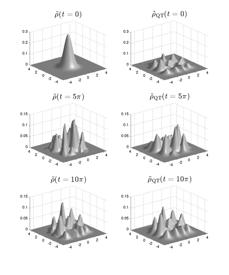
As with previous simulations, by eye the relaxation towards equilibrium is obvious. To quantify the relaxation we plot $\bar{H}(t)$ as a function of time (in units of the period $2\pi$). This is shown in Figure 2, where values for $\bar{H}$ are calculated and plotted at every period. The three separate runs, with three different grids, yield slightly different results for $\bar{H}$ which are shown in different colours. In the displayed plot, the values obtained for each run have been joined by straight lines. We also display (as a dashed line) the best fit to an exponential function of the form

$$a\exp[-b(t/2\pi)]+c\ ,$$ (9)

with constant parameters $a$, $b$ and $c$. (We require that the best fit curve passes through the value at $t=0$.)

In Figure 3 we plot $\ln\bar{H}$ against time. There we display error bars at each time, whose limits are the extremal values of the three results for $\ln\bar{H}$, and the centres of the error bars are joined by straight lines. From Figure 3 we may see that the decay is approximately exponential. However, the rate of decay during the final two periods is arguably slightly larger than during the preceding three periods – in contrast with the results of ref. [21] in which the decay rate was slightly smaller in the final two periods. To within slight variations in the decay rate, we may say that for $M=25$ we have confirmed an approximately exponential decay over five periods. We also see that $\bar{H}$ drops from an initial value $\simeq 1.26$ to a final (mean) value $\simeq 0.01$. The final value is less than $1\%$ of the initial value. (The final value of $\bar{H}$ is significantly smaller than in ref. [21] because here the coarse-graining length is larger.)

As shown in Figure 2 the best-fit curve for $\bar{H}(t)$ has a small ‘residue’

$$\bar{H}_{\mathrm{res}}=c\simeq 0.02$$ (10)

equal to about $2\%$ of the initial value. However, this is comparable to the error (the differences in the three values obtained at four and five periods) and so we are unable to say if the residue is real or significant.

Figure 2: Plots of the coarse-grained $H$-function $\bar{H}(t)$ as a function of time (in units of the period $2\pi$), for 25 energy states. Three separate simulations with three different grids yield slightly different results for $\bar{H}$ (shown in different colours). In the display, the values obtained have been joined by straight lines and we include (dashed line) a best fit to an exponential with a residue. The residue $c$ is comparable to the error.

Figure 3: Plot of $\ln\bar{H}$ against time for a case with 25 energy states. The error bars indicate the extremal values of the three results for $\ln\bar{H}$. In the display the centres of the error bars are joined by straight lines. The decay is approximately exponential.

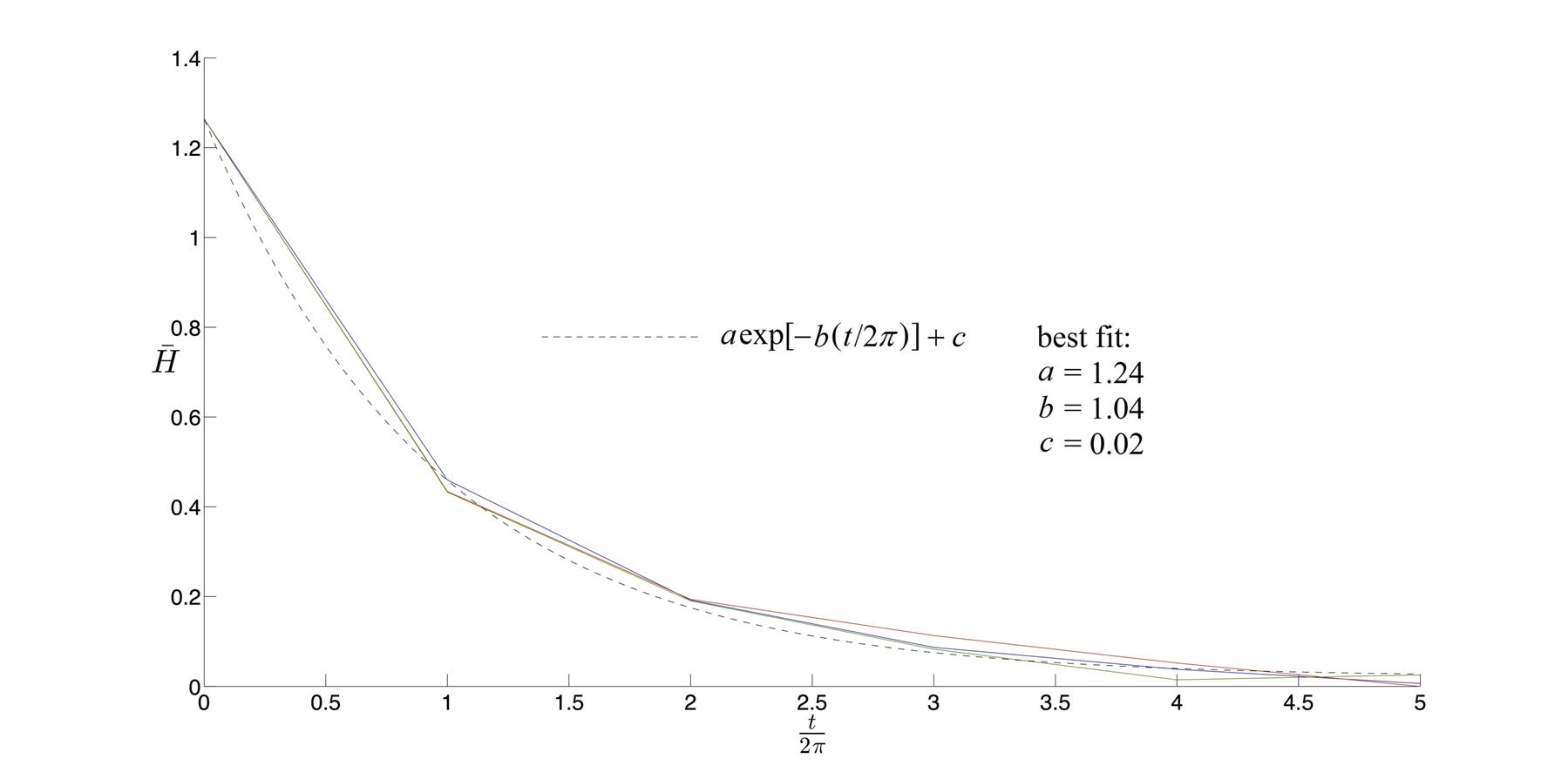
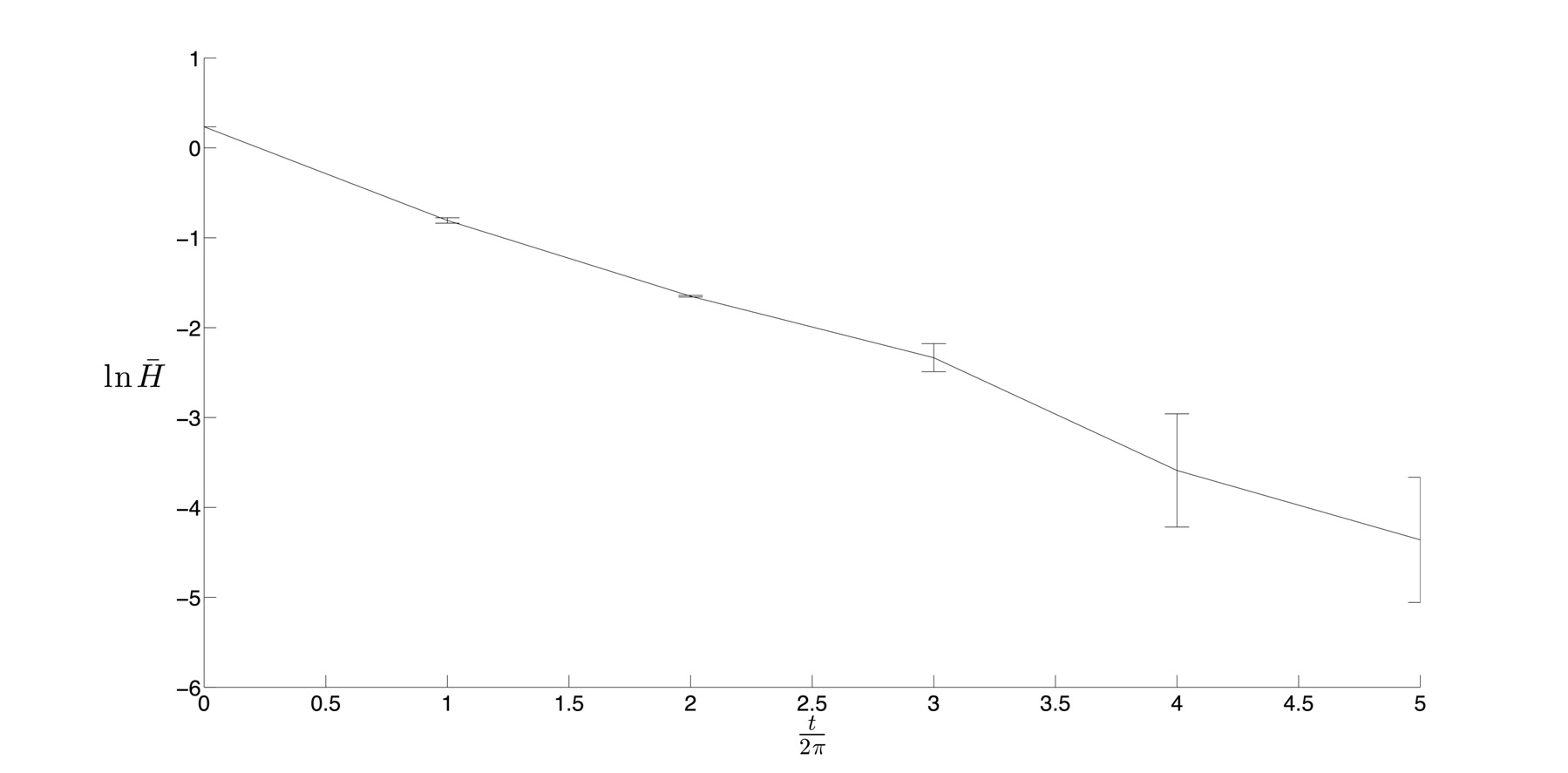
Does the decay continue indefinitely (whether exponentially or not), with $\bar{H}$ asymptotically approaching zero? Or does the decay of $\bar{H}$ halt at some point? We are unable to say, as we have been unable to calculate $\bar{H}$ accurately beyond five periods. In Figure 2 the green curve increases during the fifth period, suggesting that the decay of $\bar{H}$ may be halting. But only further simulations over longer time intervals can settle the matter. For $M=25$ the trajectories are very erratic and an accurate computation of $\bar{H}$ beyond five periods has unfortunately proved to be too difficult given our current methods. The difficulty lies not in the computational time taken to perform the simulations, but in the excessive number of inaccurate (discarded) trajectories that appear when we attempt to carry the simulations further ahead in time. We have tried increasing the maximal number of time steps per trajectory from $10^{7}$ to $10^{8}$ but with little improvement in the percentage of accurate trajectories.

As things stand, we cannot confirm that the decay halts for this case with $M=25$. However, we are able to confirm such a phenomenon for a case with $M=4$.

4 An example of long-time saturation of relaxation

We now consider a case with just four energy states, $M=4$. The velocity field is much milder and the trajectories less erratic. The numerical simulation is therefore considerably easier and we are able to find accurate results for $\bar{H}$ up to 50 periods (as opposed to just five periods for $M=25$).

A three-dimensional plot of our results is now displayed in Figure 4, where again the smoothed nonequilibrium density $\tilde{\rho}$ is shown in the left-hand column and the smoothed equilibrium density $\tilde{\rho}_{\mathrm{QT}}$ is shown in the right-hand column. The first row shows the densities at the initial time $t=0$, while the third row shows the densities at the final time $t=100\pi$ (after 50 periods). The second row shows the densities at the intermediate time $t=50\pi$.

Figure 4: Saturation of relaxation for a case with four energy states. Again, the left-hand column shows the (smoothed) nonequilibrium density $\tilde{\rho}$ and the right-hand column shows the (smoothed) equilibrium density $\tilde{\rho}_{\mathrm{QT}}$. The first, second and third rows show the densities at the respective times $t=0$, $50\pi$ and $100\pi$ (up to 50 periods).

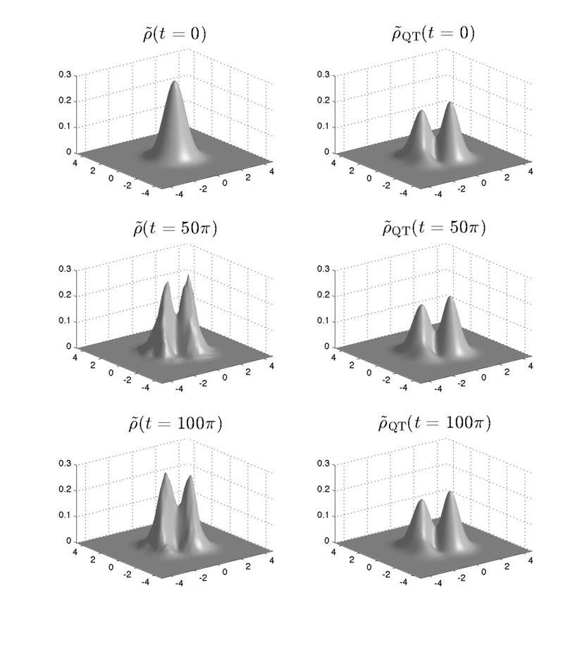
Remarkably – for such a tiny number of modes – by eye one can still see a clear relaxation towards equilibrium. The quantum state is of the very simple form $\sim\left|00\right\rangle+\left|01\right\rangle+\left|10\right\rangle+\left|11\right\rangle$ (with randomly-chosen relative initial phases). And yet, with such a minimal number of excitations above the ground state, very significant relaxation still occurs if only one waits a sufficiently long time. Furthermore, at least initially, the coarse-grained function $\bar{H}(t)$ still decays approximately exponentially with time.

However, as shown in Figures 5 and 6 (where we respectively plot $\bar{H}$ and $\ln\bar{H}$ against time), the decay of $\bar{H}$ is approximately exponential only for the first 15 or 20 periods. (For the first 15 periods values for $\bar{H}$ are calculated and plotted every period. Thereafter we have one value at 20 periods and subsequently every 10 periods up until 50 periods. As before, at each time there are three different values of $\bar{H}$ obtained from three different grids, hence the error bars.)

Figure 5 again includes a best-fit to an exponential decay with a residue, of the form (9). In this case the residue is significantly larger than the error (the differences in the three values obtained, in particular at 40 and 50 periods). The residue appears to be real and significant.

Figure 5: Plots of $\bar{H}(t)$ as a function of time for a case with just four energy states. Again, three separate simulations yield slightly different results for $\bar{H}$ and we include (dashed line) a best fit to an exponential with a residue. The residue $c$ is now larger than the error. The decay appears to saturate after about 20 periods ($t_{\mathrm{sat}}\simeq 40\pi$).

Figure 6: Plot of $\ln\bar{H}$ against time for a case with four energy states. Again, the error bars indicate the extremal values of the three results for $\ln\bar{H}$ and the centres of the error bars are joined by straight lines. The decay is approximately exponential only for the first 15 or 20 periods.

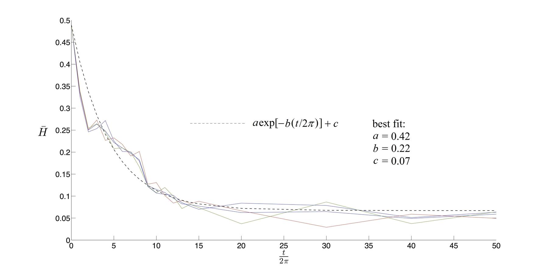
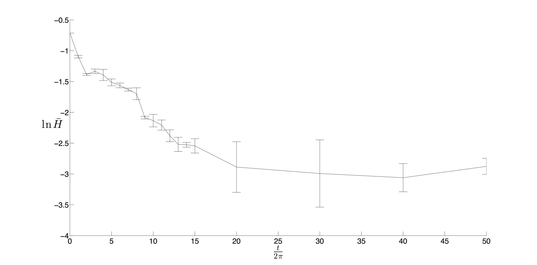
Thus, after about 20 periods ($t=40\pi$) the decay appears to halt: the function $\bar{H}(t)$ levels off (roughly) to a constant residue

$$\bar{H}_{\mathrm{res}}=c\simeq 0.07\ .$$ (11)

As we can see from Figure 5, $\bar{H}$ has dropped from an initial value $\simeq 0.49$ to a final (mean) value $\simeq 0.06$ – the final value is about $12\%$ of the initial value. After as much as an additional 30 periods the residue shows no sign of disappearing, and it seems reasonable to suppose that no further relaxation (as measured by the decrease of $\bar{H}$) will take place.

For this case with four energy states, then, it appears that the exponential decay levels off after about 15 or 20 periods, with a residue that exceeds $10\%$ of the initial value. We may say that relaxation halts after about a ‘saturation time’

$$t_{\mathrm{sat}}\simeq 40\pi\ .$$ (12)

For all we know there may exist a (smaller) residue for the above case with $M=25$ as well – setting in at some time larger than the five periods we have been able to calculate for. To settle this would require accurate simulations over longer times for that case.

5 Confinement of trajectories

To understand these results, we study the ‘confinement’ of the trajectories – the tendency for them to remain within sub-regions of configuration space instead of exploring the whole support of $\left|\psi\right|^{2}$. We use two simple but effective tests. First, we plot examples of single trajectories obtained by evolving continuously forwards in time over many periods. Second, we consider a selection of small (square) regions filled with a large number of initial points, and we plot the final positions of those points at a single final time (to show the ‘fate’ of an initial square after many periods). The first test gives a visual sense of the degree to which trajectories explore the support of $\left|\psi\right|^{2}$, while the second test gives a visual sense of the degree to which neighbouring initial points become widely scattered.

We first consider the case $M=25$, with the same initial wave function (including phases) that was used in Section 3.

In Figure 7a we display trajectories obtained from a selection of 10 initial points, evolved from $t=0$ to $t=10\pi$ (five periods). In Figure 7b we display 10 initial squares at $t=0$ (each containing 100 points) and their fate at $t=10\pi$. (The squares are centred on the 10 initial points used previously.)

Figure 7: For the case $M=25$ (as in Section 3) we display (a) trajectories, and (b) the fate of initial small squares, each calculated over five periods. There is negligible confinement. (In (b), each of the initial squares yields scattered final points only, with no ‘streaks’ or other evident clustering.)

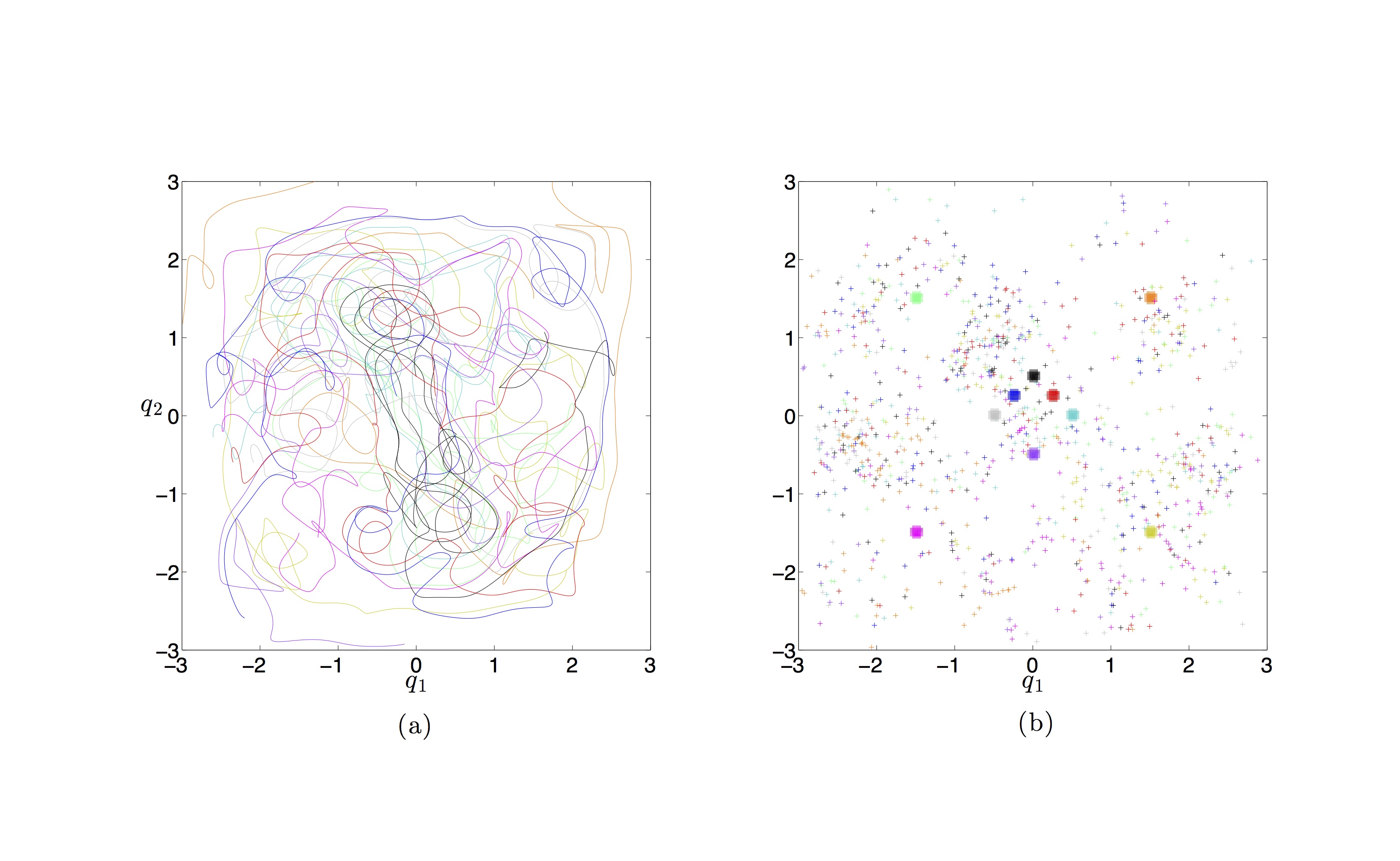
The trajectories show negligible confinement. Instead, roughly speaking, they tend to explore more or less the whole of the support of $\left|\psi\right|^{2}$. This is consistent with the absence of a discernible residue in $\bar{H}$ for this case.

We now consider the case $M=4$, with the same initial wave function (including phases) that was used in Section 4.

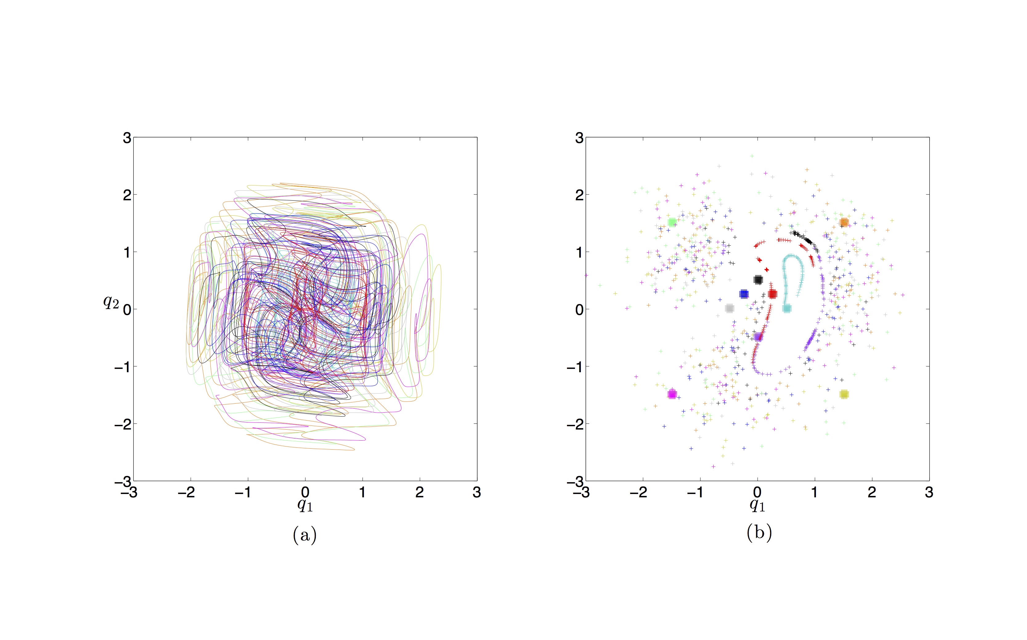
In Figure 8a we display trajectories obtained from the same selection of 10 initial points used above, now evolved from $t=0$ to $t=50\pi$ ($25$ periods). In Figure 8b we display the same 10 initial squares at $t=0$ and their fate at $t=50\pi$.

Figure 8: For the case $M=4$ (as in Section 4) we display (a) trajectories, and (b) the fate of initial small squares, each calculated over $25$ periods. There is strong confinement. (In (b), four squares yield clustered streaks only (black, dark blue, red, light blue), one yields a streak and scattered points (grey), five yield scattered points only (green, yellow, gold, purple, magenta).)

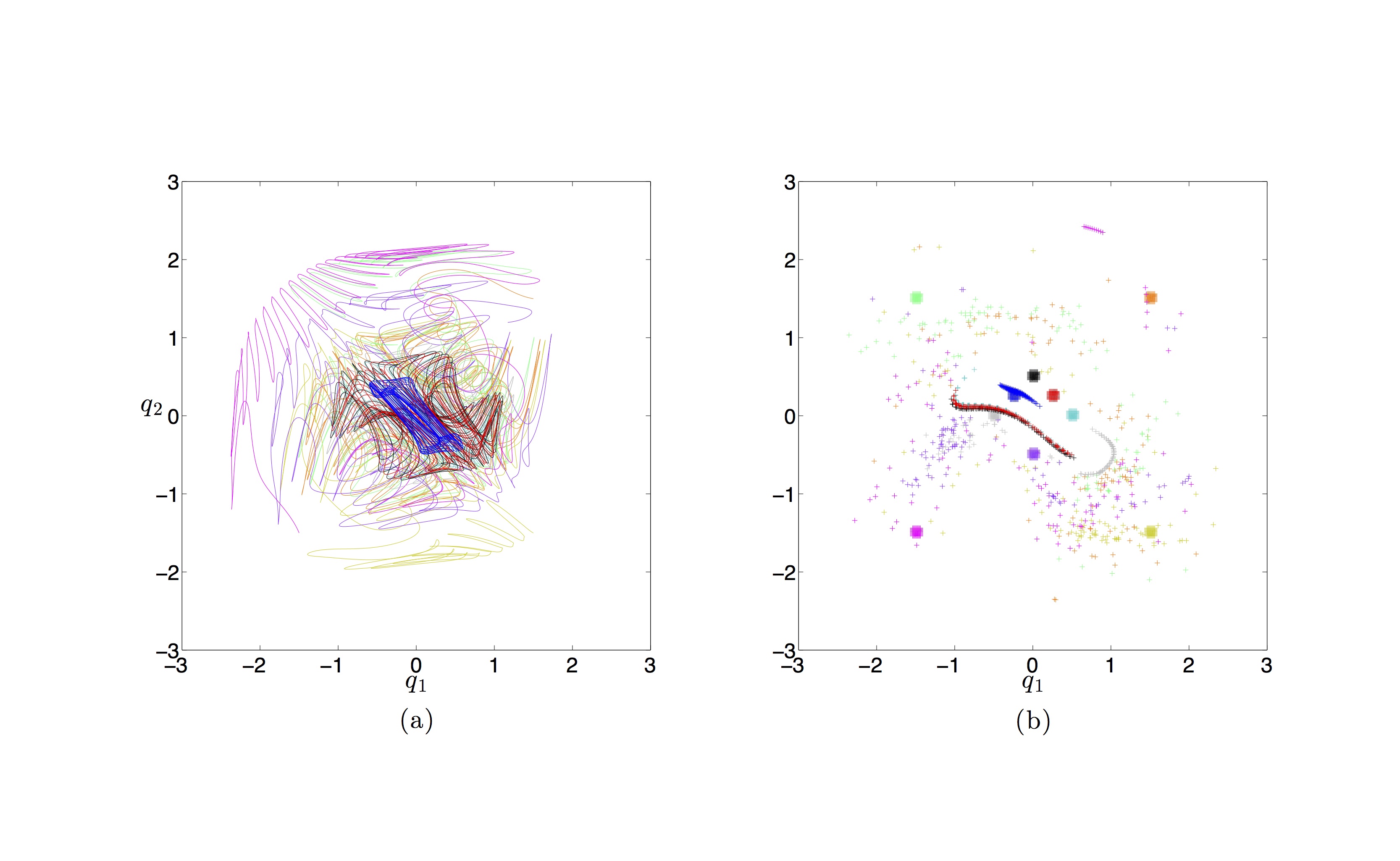
The trajectories now show a strong tendency to be confined. They do not generally explore the whole of the support of $\left|\psi\right|^{2}$. This is consistent with the presence of a large residue in $\bar{H}$ for this case.

So far we have only considered a particular choice of initial phases for each case, $M=25$ and $M=4$. In the first case the trajectories tend to explore the support of $\left|\psi\right|^{2}$ and there is no discernible residue in $\bar{H}$. In the second case the trajectories tend to be confined and there is a definite large residue in $\bar{H}$. How common is this behaviour for different choices of initial phases? Some straightforward tests show that confinement is more likely to occur for low values of $M$ and less likely to occur for high values of $M$ (assuming that the initial phases are chosen randomly).

To see this we examine similar plots – of trajectories and of the fate of initial squares – for different sets of randomly-chosen initial phases and for varying values of $M$. Specifically, we have plotted trajectories obtained from the same selection of ten initial points as above, but with ten different sets of initial phases. This has been done for each of $M=4,\ 9,\ 16$ and $25$ (with final times $t=50\pi$, $20\pi$, $15\pi$ and $10\pi$ respectively). We have also plotted the fates of the same ten initial squares as above, again with ten different sets of initial phases and for each of $M=4,\ 9,\ 16$ and $25$ (again with the listed final times).

For $M=4$ we find that about two thirds of cases – where each case corresponds to a different set of initial phases – show strong confinement (comparable to that seen in Figure 8) while about one third show only mild confinement. An example of ‘mild’ confinement is shown in Figure 9. For $M=9$ about half of the cases show strong to mild confinement; while for about half of the cases confinement is negligible (comparable to that seen in Figure 7). For $M=16$ about half of the cases show mild to low confinement; while for about half of the cases confinement is negligible. For $M=25$, about one third of the cases show mild confinement; for about two thirds of the cases confinement is negligible.

Figure 9: An example of mild confinement for $M=4$, showing (a) trajectories, and (b) the fate of initial small squares, each calculated over $25$ periods. (In (b), two squares yield clustered streaks only (light blue, purple), one yields a long streak with some scatter (red), seven yield scattered points only (green, magenta, grey, black, dark blue, yellow, gold).)

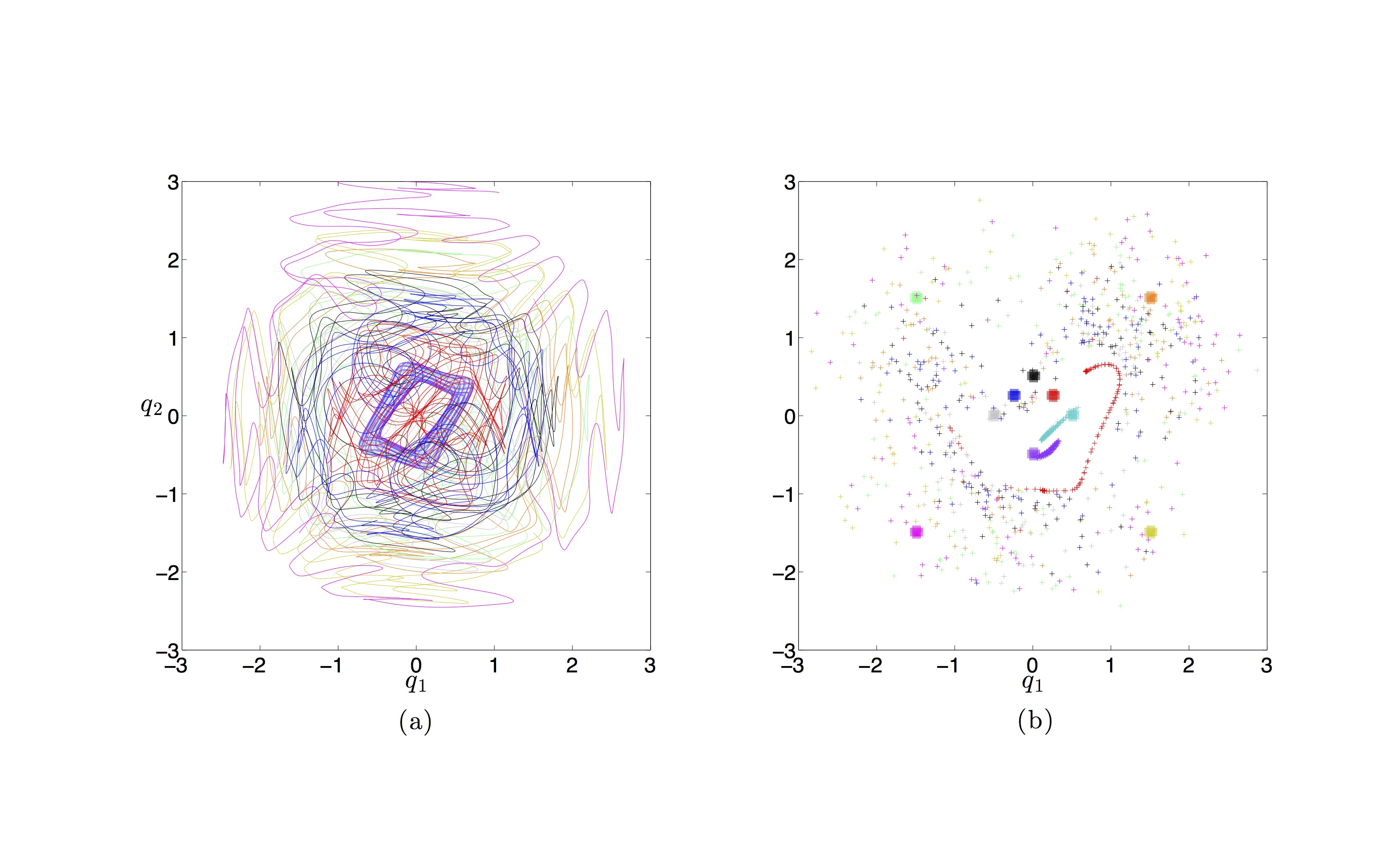
We have not attempted to quantify the degree of confinement precisely. For the present purpose it suffices to make a judgement by eye from the plots, which show a clear tendency for stronger confinement at lower $M$ and milder or negligible confinement at larger $M$.

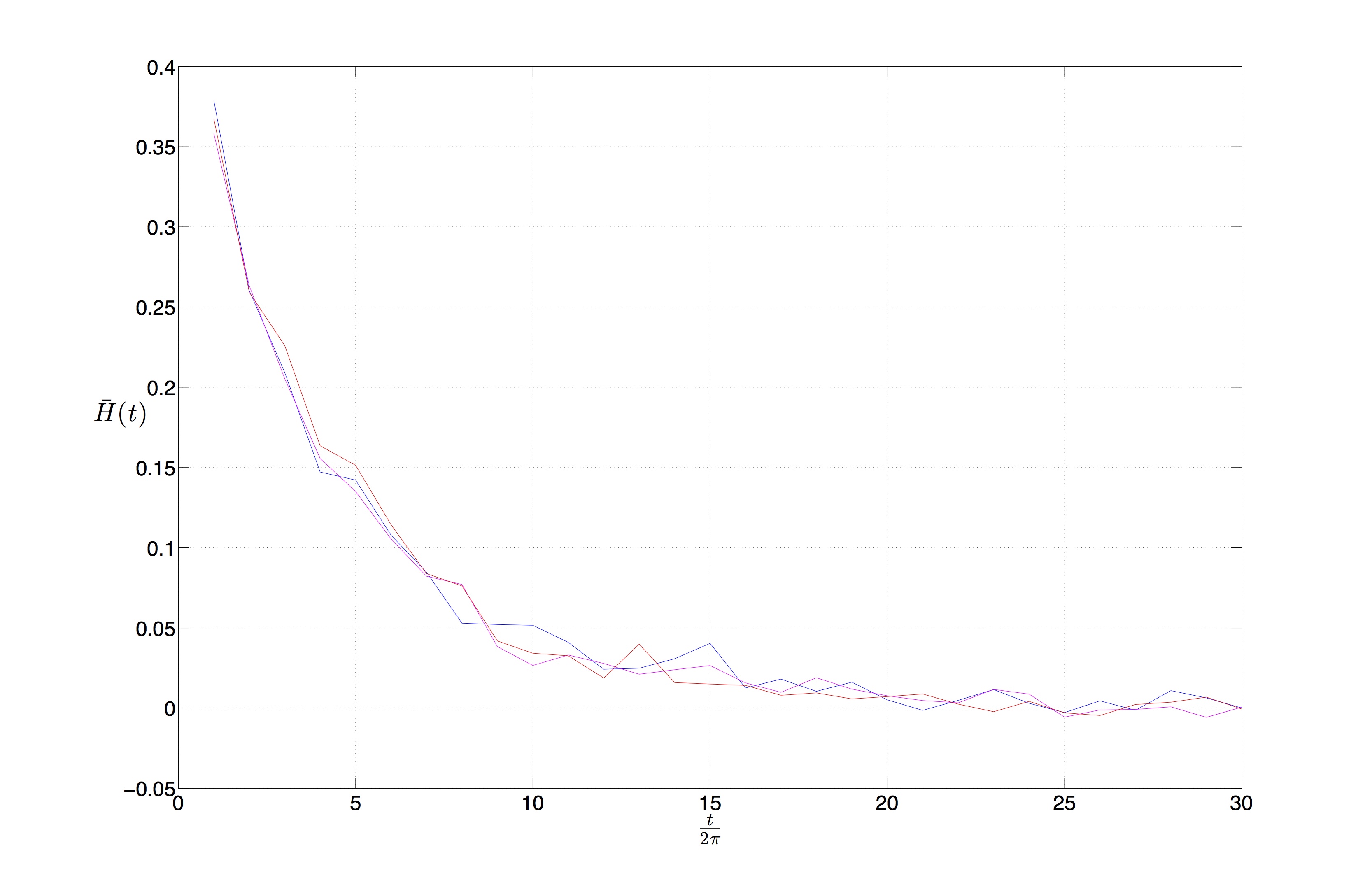
For $M=4$, while most choices of initial phases yield strong confinement some do not. In a latter case we would expect there to be a smaller residue in $\bar{H}$ or perhaps no discernible residue at all. This has been confirmed by running simulations for $\bar{H}$ as done in Section 4 but with a different set of initial phases chosen such that the trajectories show only a small amount of confinement. The results of our confinement tests for this case are shown in Figure 10. We find no discernible residue in $\bar{H}$. After a time evolution of $30$ periods, the value of $\bar{H}$ is indistinguishable from zero (to within the accuracy of our simulations), as shown in Figure 11.

Figure 10: For $M=4$, with selected initial phases yielding only a small amount of confinement (calculated over $25$ periods). (In (b), one square yields a clustered streak only (red), three yield both streaks and scattered points (black, light blue, purple), while six yield scattered points only (dark blue, green, yellow, gold, magenta, grey).)

Figure 11: Simulations of $\bar{H}(t)$ for $M=4$, with a set of initial phases chosen such that the trajectories show only a small amount of confinement. After $30$ periods, there is no discernible residue in $\bar{H}$.

Similarly, for $M=25$, while most choices of initial phases yield negligible confinement some choices do not. In a case with significant confinement we may expect to find a residue in $\bar{H}$.

While there is clearly room for further and more quantitative study, we may draw the following broad conclusions. As the number $M$ of energy states increases, we are less likely to find confinement of the trajectories; it is more likely that the trajectories will explore the bulk of the support of $\left|\psi\right|^{2}$. (The measure of ‘likelihood’ is defined by choosing the initial phases randomly on the unit circle, where each choice of phases corresponds to a choice of initial wave function.) A large or significant residue in $\bar{H}$ is then more likely to exist for smaller $M$ and less likely to exist for larger $M$. A precise study of how the likelihood diminishes with $M$ is left for future work.

6 Conclusion

For a superposition of 25 energy states we have confirmed an approximately exponential decay of the coarse-grained $H$-function $\bar{H}(t)$ to a final value that is less than $1\%$ of the initial value (after five periods of periodic wave function evolution, the limit beyond which we were unable to calculate $\bar{H}$ accurately). In contrast, for a case with just four energy states we were able to calculate much further in time, and we found that the approximately exponential decay of $\bar{H}(t)$ halts or saturates after a time $t_{\mathrm{sat}}$ equal to about 20 periods or so, with a large residue $\bar{H}_{\mathrm{res}}$ that exceeds $10\%$ of the initial value $\bar{H}(0)$. For the latter case we were able to calculate $\bar{H}$ accurately for an additional 30 periods – that is, up to a total of 50 periods – and we have confirmed that the residue shows no sign of disappearing. We are able to explain these different results in terms of the extent to which the trajectories explore the full support of $\left|\psi\right|^{2}$. In the first case the trajectories show negligible confinement to sub-regions of configuration space, whereas in the second case the trajectories show strong confinement. The lack of full exploration of the support of $\left|\psi\right|^{2}$ in the second case explains why we obtain a large residue $\bar{H}_{\mathrm{res}}$. We also found a case with four energy states for which the trajectories show only a small amount of confinement and $\bar{H}(t)$ becomes indistinguishable from zero (to the accuracy of our simulations). We have studied how common the two kinds of behaviour are likely to be, for different wave functions with randomly-chosen initial phases. We conclude that the confinement of trajectories – and an associated large residue $\bar{H}_{\mathrm{res}}$ – are less likely to occur when the initial wave function contains a larger number $M$ of energy states.

Many open questions remain. It may be that for any given $M$, no matter how large, significant confinement and an associated large residue $\bar{H}_{\mathrm{res}}$ always exist for some sets of initial phases – though we would expect such sets to become increasingly rare as $M$ increases. On the other hand, it seems conceivable that if $M$ exceeds a critical value $M_{\mathrm{crit}}$ there will be no significant confinement regardless of the initial set of phases. We hope that further study will clarify this. Even in the absence of significant confinement, there could still exist a small residue $\bar{H}_{\mathrm{res}}$ at sufficiently large times $t_{\mathrm{sat}}$. For all we know this could be true for any finite $M$. If so, we would like to know how $t_{\mathrm{sat}}$ and $\bar{H}_{\mathrm{res}}$ scale with $M$. Presumably $\bar{H}_{\mathrm{res}}$ will decrease with increasing $M$, since the increased complexity of the velocity field makes the trajectories more erratic and so will drive the system closer to equilibrium. The same may be true for $t_{\mathrm{sat}}$. (Note that we have discussed relaxation in terms of a coarse-graining approach for isolated systems [7, 9, 11], modelled on the analogous classical discussion [36, 37]. If a residue $\bar{H}_{\mathrm{res}}$ does always exist for any finite $M$, this might be viewed as an artifact of treating the system as strictly isolated.) On the other hand, again, it seems conceivable that if $M$ exceeds some other critical value $M_{\mathrm{crit}}^{\prime}$ there will be a continued exponential decay of $\bar{H}(t)$ asymptotically to zero. These are tantalising open questions that require further study, perhaps with improved numerical methods.

Finally, we briefly address possible cosmological consequences.

For ordinary systems emerging from a hot big bang, at early times there will have been a huge number $M$ of energy states superposed in the relevant wave functions, and so any residue $\bar{H}_{\mathrm{res}}$ today (if there is such) is likely to be extremely small – presumably corresponding to a residual nonequilibrium at a very tiny lengthscale (as originally suggested in ref. [9]). Perhaps this lengthscale is so small, for the overwhelming majority of sets of initial phases, as to be essentially unobservable. Only improved simulations will be able to settle the matter. (In contrast, for relic particles that decoupled sufficiently early, it is conceivable that deviations from equilibrium exist on quite large scales today; see refs. [11, 13, 14].)

On the other hand, our results for $M=4$ show that a large residue $\bar{H}_{\mathrm{res}}$ is likely to exist if the number of excitations was always sufficiently small. A system with such a small number of excitations would not be expected to have ever existed at high temperatures in the early universe. However, as we have mentioned, it is possible that there was a pre-inflationary era with very few excitations above the vacuum. Our results suggest that, even if such an era lasts a very long time, there is likely to be a significant residual nonequilibrium during inflation at all relevant wavelengths (and not only at long wavelengths owing to the suppression of relaxation discussed in refs. [13, 14, 16, 21]).

Acknowledgements. A.V. is grateful to Patrick Peter for helpful discussions. The work of A.V. and S.C. was funded jointly by the John Templeton Foundation and Clemson University.

References

- [1] L. de Broglie, in: Électrons et Photons: Rapports et Discussions du Cinquième Conseil de Physique (Gauthier-Villars, Paris, 1928). [English translation in ref. [2].]
- [2] G. Bacciagaluppi and A. Valentini, Quantum Theory at the Crossroads: Reconsidering the 1927 Solvay Conference (Cambridge University Press, 2009). [arXiv:quant-ph/0609184]
- [3] D. Bohm, Phys. Rev. 85, 166 (1952).
- [4] D. Bohm, Phys. Rev. 85, 180 (1952).
- [5] P. R. Holland, The Quantum Theory of Motion: an Account of the de Broglie-Bohm Causal Interpretation of Quantum Mechanics (Cambridge University Press, Cambridge, 1993).
- [6] W. Struyve and A. Valentini, J. Phys. A: Math. Theor. 42, 035301 (2009). [arXiv:0808.0290]
- [7] A. Valentini, Phys. Lett. A 156, 5 (1991).
- [8] A. Valentini, Phys. Lett. A 158, 1 (1991).
- [9] A. Valentini, PhD thesis, International School for Advanced Studies, Trieste, Italy (1992). [https://digitallibrary.sissa.it/bitstream/handle/1963/5424/PhD_Valentini_Antony.pdf?sequence=1]
- [10] A. Valentini, in: Bohmian Mechanics and Quantum Theory: an Appraisal, eds. J. T. Cushing et al. (Kluwer, Dordrecht, 1996).
- [11] A. Valentini, in: Chance in Physics: Foundations and Perspectives, eds. J. Bricmont et al. (Springer, Berlin, 2001). [arXiv:quant-ph/0104067]
- [12] A. Valentini, Pramana – J. Phys. 59, 269 (2002). [arXiv:quant-ph/0203049]
- [13] A. Valentini, J. Phys. A: Math. Theor. 40, 3285 (2007). [arXiv:hep-th/0610032]
- [14] A. Valentini, De Broglie-Bohm prediction of quantum violations for cosmological super-Hubble modes, arXiv:0804.4656 [hep-th].
- [15] A. Valentini, Physics World 22N11, 32 (2009). [arXiv:1001.2758]
- [16] A. Valentini, Phys. Rev. D 82, 063513 (2010). [arXiv:0805.0163]
- [17] P. Pearle and A. Valentini, in: Encyclopaedia of Mathematical Physics, eds. J.-P. Françoise et al. (Elsevier, North-Holland, 2006). [arXiv:quant-ph/0506115]
- [18] A. Valentini and H. Westman, Proc. Roy. Soc. Lond. A 461, 253 (2005). [arXiv:quant-ph/0403034]
- [19] M. D. Towler, N. J. Russell, and A. Valentini, Proc. Roy. Soc. Lond. A 468, 990 (2012). [arXiv:1103.1589]
- [20] S. Colin, Proc. Roy. Soc. Lond. A 468, 1116 (2012). [arXiv:1108.5496]
- [21] S. Colin and A. Valentini, Phys. Rev. D 88, 103515 (2013). [arXiv:1306.1579 [hep-th]]
- [22] G. Contopoulos, N. Delis and C. Efthymiopoulos, J. Phys. A: Math. Theor. 45, 165301 (2012).
- [23] C. Efthymiopoulos and G. Contopoulos, J. Phys. A: Math. Gen. 39, 1819 (2006).
- [24] A. R. Liddle and D. H. Lyth, Cosmological Inflation and Large-Scale Structure (Cambridge University Press, Cambridge, 2000).
- [25] V. Mukhanov, Physical Foundations of Cosmology (Cambridge University Press, Cambridge, 2005).
- [26] S. Weinberg, Cosmology (Oxford University Press, 2008).
- [27] P. Peter and J.-P. Uzan, Primordial Cosmology (Oxford University Press, 2009).
- [28] A. Valentini, Hidden Variables in Modern Physics and Beyond (Cambridge University Press, forthcoming).
- [29] A. Vilenkin and L. H. Ford, Phys. Rev. D 26, 1231 (1982).
- [30] A. D. Linde, Phys. Lett. B 116, 335 (1982).
- [31] A. A. Starobinsky, Phys. Lett. B 117, 175 (1982).
- [32] B. A. Powell and W. H. Kinney, Phys. Rev. D 76, 063512 (2007).
- [33] I.-C. Wang and K.-W. Ng, Phys. Rev. D 77, 083501 (2008).
- [34] Planck Collaboration: P. A. R. Ade et al., Planck 2013 results. XV. CMB power spectra and likelihood, arXiv:1303.5075.
- [35] S. Colin and W. Struyve, New J. Phys. 12, 043008 (2010).
- [36] R. C. Tolman, The Principles of Statistical Mechanics (Dover, New York, 1979).
- [37] P. C. W. Davies, The Physics of Time Asymmetry (University of California Press, Berkeley, 1974).