Limits on anisotropic inflation from the Planck data
Abstract
Temperature anisotropy of the cosmic microwave background offers a test of the fundamental symmetry of spacetime during cosmic inflation. Violation of rotational symmetry yields a distinct signature in the power spectrum of primordial fluctuations as , where is a preferred direction in space and is an amplitude. Using the Planck 2013 temperature maps, we find no evidence for violation of rotational symmetry, (68% CL), once the known effects of asymmetry of the Planck beams and Galactic foreground emission are removed.
pacs:
98.70.Vc, 98.80.Cq, 98.80.-kCosmic inflation Starobinsky (1980); Sato (1981); Guth (1981); Linde (1982); Albrecht and Steinhardt (1982), an indispensable building-block of the standard model of the universe, is described by nearly de Sitter spacetime. The metric charted by flat coordinates is given by , where is the expansion rate of the universe during inflation. This spacetime admits ten isometries: three spatial translations; three spatial rotations; one time translation accompanied by spatial dilation ( and with a constant ); and three additional isometries which reduce to special conformal transformations in . The necessary time-dependence of the expansion rate, , breaks the time translation symmetry hence the spatial dilation symmetry, yielding the two-point correlation function of primordial fluctuations that is nearly, but not exactly, invariant under Mukhanov and Chibisov (1981). The magnitude of the deviation from dilation invariance is limited by that of the time-dependence of , i.e., .
In the usual model of inflation, six out of ten isometries remain unbroken: translations and rotations. Why must they remain unbroken while the others are broken? In this paper, we shall test rotational symmetry during inflation, using the two-point correlation function of primordial perturbations to spatial curvature, , generated during inflation. This is defined as a perturbation to the exponent in the spatial metric, . In Fourier space, we write the two-point function as , and is the power spectrum. Translation invariance, which is kept in this paper, gives the delta function, while rotation invariance, which is not kept, would give with . Dilation invariance would give , whereas a small deviation, , has been detected from the CMB data with more than 5- significance Hinshaw et al. (2013); Ade et al. (2013a).
Following Ref. Ackerman et al. (2007), we write the power spectrum as , where is a preferred direction in space, is a parameter characterizing the amplitude of violation of rotational symmetry, and is an isotropic power spectrum which depends only on the magnitude of the wavenumber, . This form is generic, as it is the leading-order anisotropic correction that remains invariant under parity flip, . “Anisotropic inflation” models, in which a scalar field is coupled to a vector field (see Ref. Soda (2012); Maleknejad et al. (2013); Dimastrogiovanni et al. (2010) and references therein) can produce this form.111Anisotropic inflation models produce three-point functions of which also depend on Barnaby et al. (2012); Bartolo et al. (2013); Shiraishi et al. (2013). The Planck team uses this property to put model-dependent constraints on from non-detection of primordial three-point functions Ade et al. (2013b). A very long-wavelength perturbation on super-horizon scales can also produce this form via a three-point function Schmidt and Hui (2013). A pre-inflationary universe was probably chaotic and highly anisotropic, and thus a remnant of the pre-inflationary anisotropy may still be detectable Bartolo et al. (2013).
We shall ignore a potential dependence of in this paper. We expand using spherical harmonics:
| (1) |
We then write the power spectrum as
| (2) |
where we have absorbed into the normalization of the isotropic part, , and defined with for given by .
There are 5 parameters to be determined from the data. We denote the parameter vector as . We search for in the covariance matrix of the spherical harmonics coefficients of CMB temperature maps, , where . The anisotropic power spectrum of Eq. 2 gives Ma et al. (2011)
| (7) | |||||
where the matrices denote the Wigner 3- symbols, and with the temperature radiation transfer function.
In the limit of weak anisotropy, the likelihood of the CMB data given a model may be expanded as
| (8) | |||||
The first and second derivatives are given by
| (9) | |||||
| (10) |
where , and denotes measured from the data and , both of which include noise and the other data-specific terms.
We obtain an estimator for by maximizing the likelihood with respect to Hanson and Lewis (2009)
| (11) | |||||
| (12) |
The covariance matrix, , is neither diagonal in pixel nor harmonic space. In order to reduce the computational cost, we shall approximate it as diagonal in harmonic space. While this approximation makes our estimator sub-optimal, it remains un-biased. The new estimator is
where is the spherical harmonic coefficients computed from a masked temperature map ( in the masked pixels, and 1 otherwise), and and are the signal and noise power spectra, respectively. The matrix is defined by
| (14) |
with the fraction of unmasked pixels. Here, in Eq. Limits on anisotropic inflation from the Planck data is the “mean field,” which is non-zero even when . Data-specific issues such as an incomplete sky coverage, inhomogeneous noise, and asymmetric beams generate the mean field.
From , we need to estimate and . As the estimator consists of the sum of many pairs of coefficients , we expect the estimated value to follow a Gaussian distribution (the central limit theorem). Therefore, the likelihood of and is
where is the covariance matrix of , which we compute from 1000 Monte Carlo simulations. Since has nonlinear dependence on and , we obtained the posterior distribution of and by evaluating Eq. Limits on anisotropic inflation from the Planck data with the Markov Chain Monte Carlo sampling Lewis and Bridle (2002).222One can calculate the expected error bars on using the Fisher matrix Pullen and Kamionkowski (2007). While such simplified calculations predict the same error bars on all components of , the actual error bars depend on due to the shape of the mask. Also, the Fisher calculations assume homogeneous noise. Nonetheless, our error bars on from Monte Carlo simulations and our own Fisher calculations assuming homogeneous noise and the sky fraction of 71% are in agreement, to within 20%.
We use the Planck 2013 temperature maps at , which are available at the Planck Legacy Archive Ade et al. (2013c); Aghanim et al. (2013a); Ade et al. (2013d). (We upgrade the low-frequency maps, which are originally at , to .) We use the map at 143 GHz as the main “CMB channel”, and use the other frequencies as “foreground templates”. We reduce the diffuse Galactic foreground emission by fitting templates to, and removing them from, the 143 GHz map. This is similar to the method called SEVEM by the Planck collaboration Ade et al. (2013e). We derive the templates by taking a difference between two maps at neighboring frequencies. This procedure ensures the absence of CMB in the derived templates, producing five templates: , , , , and [GHz]. To create these difference maps, we first smooth a pair of maps to the common resolution. We smooth the low-frequency maps at 30–70 GHz as , where is the beam transfer function at a frequency Aghanim et al. (2013b) and is a Gaussian beam of (FWHM). We smooth the high-frequency maps at 217–857 GHz as , where is the beam transfer function at 143 GHz Ade et al. (2013f).
After the smoothing, we mask the locations of point sources and the brightest region near the Galactic center (3% of the sky) following SEVEM Ade et al. (2013e). As the smoothed sources occupy more pixels, we enlarge the original point-source mask as follows: we create a map having at the source locations and 0 otherwise, and smooth it. We then mask the pixels whose values exceed . We fit the templates to the 143 GHz map on the unmasked pixels (86% of the sky).
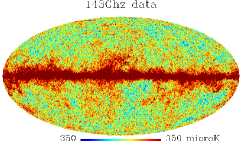
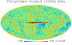
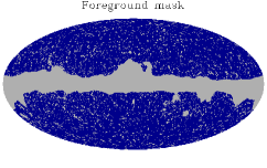
The left and middle panels of Figure 1 show the original and foreground-reduced maps at 143 GHz, respectively. We still find significant foreground emission on the Galactic plane. We thus mask the regions contaminated by the residual foreground emission, combining the masks of various foreground-reduced maps produced by the Planck collaboration (NILC, Ruler, SEVEM, and SMICA Ade et al. (2013e)), and the point-source mask. We show the combined mask in the right panel of Figure 1, which leaves 71% of the sky unmasked, and is similar to the “union mask” of the Planck collaboration, except for a slightly enlarged point-source mask due to smoothing.
We use Eqs. Limits on anisotropic inflation from the Planck data and Limits on anisotropic inflation from the Planck data to compute from the masked foreground-reduced map. We restrict our analysis to the multipole range of . We compute the mean field from 1000 Monte-Carlo realizations of signal and noise. The signal map is , where is the best-fit “Planck+WP” power spectrum Ade et al. (2013a), the pixel window function, and a Gaussian random variable with unit variance. The noise map is , where is the noise variance map provided by the Planck collaboration, and a Gaussian random variable with unit variance. We create high-frequency maps at , while we create low-frequency maps at and upgrade to . We also compute from the signal plus noise simulations, and compute the covariance matrix, , in Eq. Limits on anisotropic inflation from the Planck data. Finally, we compute the posterior distribution of and by evaluating Eq. Limits on anisotropic inflation from the Planck data using the CosmoMC sampler Lewis and Bridle (2002).
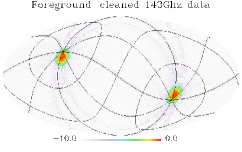
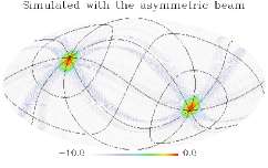
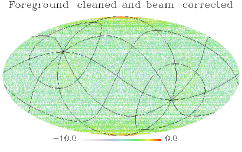
The left panel of Figure 2 shows the log-likelihood of locations of a preferred direction, , given the Planck data. We find a significant detection of (68% CL) with pointing to in Galactic coordinates. This direction lies close to the Ecliptic pole at .
This is essentially the same result as found from the WMAP data. Following the first detection reported in Ref. Groeneboom and Eriksen (2009), the subsequent analysis finds with from the WMAP 5-year map at 94 GHz in the multipole range of Groeneboom et al. (2010) (also see Hanson and Lewis (2009)). They find a negative value at 41 GHz, . These signals, however, have been explained entirely by the effect of WMAP’s asymmetric beams coupled with the scan pattern Hanson et al. (2010); Bennett et al. (2013). To confirm their results, we use the foreground-reduced WMAP 9-year maps Bennett et al. (2013), finding , , and at 41, 61, and 94 GHz, respectively, in the multipole range of . The directions lie close to the Ecliptic pole.
We find from the Planck 143 GHz map. This is because the orientations of the semi-major axes of 143 GHz beams are nearly parallel to Planck’s scan direction Ade et al. (2013f), which lies approximately along the Ecliptic longitudes. As the beams are fatter along the Ecliptic longitudes, the Planck measures less power along the Ecliptic north-south direction than the east-west direction, yielding a quadrupolar power modulation with .333While WMAP does not scan along the Ecliptic longitudes, the scan directions cover only about 30% of possible angles on the Ecliptic equator, which are closer to being parallel to the Ecliptic longitudes. As a result, the 41 GHz maps give , as the orientations of the 41 GHz beams are nearly parallel to WMAP’s scan direction, whereas the 61 and 94 GHz maps give , as the orientations are nearly perpendicular to the scan direction Hill et al. (2009). This explanation is due to Ref. Hanson et al. (2010).
We quantify and remove the effect of beam asymmetry by computing from 1000 signal plus noise simulations, in which the signal is convolved with Planck’s asymmetric beams and scans. We have used the EffConv code, which is developed by the Planck collaboration and publicly available444http://irsa.ipac.caltech.edu/data/Planck/release_1/software with the Planck effective beam data files Mitra et al. (2011); Ade et al. (2013f). The middle panel of Figure 2 shows given the simulation data. We reproduce what we find from the real data: with (the error bars are for the average of simulations). Using this result as the mean field (i.e., in Eq. Limits on anisotropic inflation from the Planck data), we recompute , finding no evidence for (see also the right panel of Figure 2, which shows no preferred direction). Our best limit is (68% CL), (95% CL) and (99.7% CL).
We have also analyzed the foreground-reduced 100 GHz map, which has less foreground emission than the 143 GHz map. We find 28- and 7- detections of in the Ecliptic-pole directions before and after the beam asymmetry correction, respectively. The 100 GHz beam is much less symmetric than the 143 GHz one Ade et al. (2013f); thus, the beam simulation needs to be more precise for removing the asymmetry to the sufficient level. We find before the beam asymmetry correction, which is consistent with the 100 GHz beams being more elongated along Planck’s scan direction.
Finally, we study the effect of Galactic foreground emission. Using the raw 143 GHz without cleaning, we find significant anisotropy: and before and after the beam asymmetry correction, respectively. The directions lie close to the Galactic pole; thus, the foreground reduction plays an important role in nulling artificial anisotropy in the data.
| BC | FR | direction [degrees] | |
|---|---|---|---|
| No | No | ||
| Yes | No | ||
| No | Yes | ||
| Yes | Yes | ||
| No | — |
We summarize our finding in Table 1. After removing the
effects of Planck’s asymmetric beams and Galactic
foreground emission, we find no evidence for . Our limit, about 2%
in , provides the most stringent test of rotational symmetry during
inflation.
JK would like to thank Belen Barreiro, Carlo Baccigalupi, Jacques Delabrouille, Sanjit Mitra, Anthony Lewis and Niels Oppermann for helpful discussions. We acknowledge the use of the Planck Legacy Archive (PLA). The development of Planck has been supported by: ESA; CNES and CNRS/INSU-IN2P3-INP (France); ASI, CNR, and INAF (Italy); NASA and DoE (USA); STFC and UKSA (UK); CSIC, MICINN and JA (Spain); Tekes, AoF and CSC (Finland); DLR and MPG (Germany); CSA (Canada); DTU Space (Denmark); SER/SSO (Switzerland); RCN (Norway); SFI (Ireland); FCT/MCTES (Portugal); and PRACE (EU). A description of the Planck Collaboration and a list of its members, including the technical or scientific activities in which they have been involved, can be found at http://www.sciops.esa.int/index.php?project=planck&page=Planck_Collaboration. We acknowledge the use of the Legacy Archive for Microwave Background Data Analysis (LAMBDA), part of the High Energy Astrophysics Science Archive Center (HEASARC). HEASARC/LAMBDA is a service of the Astrophysics Science Division at the NASA Goddard Space Flight Center. We also acknowledge the use of the EffConv Mitra et al. (2011), HEALPix Gorski et al. (2005), CAMB Lewis et al. (2000), and CosmoMC packages Lewis and Bridle (2002).
References
- Starobinsky (1980) A. A. Starobinsky, Phys.Lett. B91, 99 (1980).
- Sato (1981) K. Sato, Mon.Not.Roy.Astron.Soc. 195, 467 (1981).
- Guth (1981) A. H. Guth, Phys.Rev. D23, 347 (1981).
- Linde (1982) A. D. Linde, Phys.Lett. B108, 389 (1982).
- Albrecht and Steinhardt (1982) A. Albrecht and P. J. Steinhardt, Phys.Rev.Lett. 48, 1220 (1982).
- Mukhanov and Chibisov (1981) V. F. Mukhanov and G. Chibisov, JETP Lett. 33, 532 (1981).
- Hinshaw et al. (2013) G. Hinshaw et al., Astrophys.J.Suppl. 208, 19 (2013), arXiv:1212.5226.
- Ade et al. (2013a) P. Ade et al. (Planck Collaboration), ArXiv e-prints (2013a), arXiv:1303.5076 [astro-ph.CO] .
- Ackerman et al. (2007) L. Ackerman, S. M. Carroll, and M. B. Wise, Phys.Rev. D75, 083502 (2007), arXiv:astro-ph/0701357 [astro-ph] .
- Soda (2012) J. Soda, Class.Quant.Grav. 29, 083001 (2012), arXiv:1201.6434 [hep-th] .
- Maleknejad et al. (2013) A. Maleknejad, M. Sheikh-Jabbari, and J. Soda, Phys.Rept. 528, 161 (2013), arXiv:1212.2921 [hep-th] .
- Dimastrogiovanni et al. (2010) E. Dimastrogiovanni, N. Bartolo, S. Matarrese, and A. Riotto, Adv.Astron. 2010, 752670 (2010), arXiv:1001.4049 [astro-ph.CO] .
- Barnaby et al. (2012) N. Barnaby, R. Namba, and M. Peloso, Phys.Rev. D85, 123523 (2012), arXiv:1202.1469 [astro-ph.CO] .
- Shiraishi et al. (2013) M. Shiraishi, E. Komatsu, M. Peloso, and N. Barnaby, JCAP 1305, 002 (2013), arXiv:1302.3056 [astro-ph.CO] .
- Bartolo et al. (2013) N. Bartolo, S. Matarrese, M. Peloso, and A. Ricciardone, Phys. Rev. D 87, 023504 (2013), arXiv:1210.3257 [astro-ph.CO] .
- Ade et al. (2013b) P. Ade et al. (Planck Collaboration), (2013b), arXiv:1303.5084 [astro-ph.CO] .
- Schmidt and Hui (2013) F. Schmidt and L. Hui, Phys.Rev.Lett. 110, 011301 (2013), arXiv:1210.2965 [astro-ph.CO] .
- Bartolo et al. (2013) N. Bartolo, S. Matarrese, M. Peloso, and A. Ricciardone, JCAP 1308, 022 (2013), arXiv:1306.4160 [astro-ph.CO] .
- Ma et al. (2011) Y.-Z. Ma, G. Efstathiou, and A. Challinor, Phys. Rev. D 83, 083005 (2011), arXiv:1102.4961 .
- Hanson and Lewis (2009) D. Hanson and A. Lewis, Phys. Rev. D 80, 063004 (2009), arXiv:0908.0963 .
- Lewis and Bridle (2002) A. Lewis and S. Bridle, Phys. Rev. D 66, 103511 (2002).
- Pullen and Kamionkowski (2007) A. R. Pullen and M. Kamionkowski, Phys. Rev. D 76, 103529 (2007), arXiv:0709.1144 .
- Ade et al. (2013c) P. Ade et al. (Planck Collaboration), ArXiv e-prints (2013c), arXiv:1303.5062 [astro-ph.CO] .
- Aghanim et al. (2013a) N. Aghanim et al. (Planck Collaboration), ArXiv e-prints (2013a), arXiv:1303.5063 [astro-ph.IM] .
- Ade et al. (2013d) P. Ade et al. (Planck Collaboration), ArXiv e-prints (2013d), arXiv:1303.5067 [astro-ph.CO] .
- Ade et al. (2013e) P. Ade et al. (Planck Collaboration), ArXiv e-prints (2013e), arXiv:1303.5072 [astro-ph.CO] .
- Aghanim et al. (2013b) N. Aghanim et al. (Planck Collaboration), ArXiv e-prints (2013b), arXiv:1303.5065 [astro-ph.CO] .
- Ade et al. (2013f) P. Ade et al. (Planck Collaboration), ArXiv e-prints (2013f), arXiv:1303.5068 [astro-ph.IM] .
- Groeneboom and Eriksen (2009) N. E. Groeneboom and H. K. Eriksen, Astrophys. J. 690, 1807 (2009), arXiv:0807.2242.
- Groeneboom et al. (2010) N. E. Groeneboom, L. Ackerman, I. Kathrine Wehus, and H. K. Eriksen, Astrophys. J. 722, 452 (2010), arXiv:0911.0150 .
- Hanson et al. (2010) D. Hanson, A. Lewis, and A. Challinor, Phys. Rev. D 81, 103003 (2010), 1003.0198 .
- Bennett et al. (2013) C. L. Bennett et al., Astrophys.J.Suppl. 208, 20 (2013), arXiv:1212.5225.
- Hill et al. (2009) R. Hill et al. (WMAP Collaboration), Astrophys.J.Suppl. 180, 246 (2009), arXiv:0803.0570 [astro-ph] .
- Mitra et al. (2011) S. Mitra, G. Rocha, K. M. Górski, K. M. Huffenberger, H. K. Eriksen, M. A. J. Ashdown, and C. R. Lawrence, Astrophys.J.Suppl. 193, 5 (2011), arXiv:1005.1929 [astro-ph.CO] .
- Gorski et al. (2005) K. M. Gorski, E. Hivon, A. J. Banday, B. D. Wandelt, F. K. Hansen, M. Reinecke, and M. Bartelman, Astrophys. J. 622, 759 (2005).
- Lewis et al. (2000) A. Lewis, A. Challinor, and A. Lasenby, Astrophys. J. 538, 473 (2000), http://camb.info/ .