Distribution of lifetimes of kinetochore-microtubule attachments:
interplay of energy landscape, molecular motors and microtubule (de-)polymerization

Abstract

Before a cell divides into two daughter cells, chromosomes are replicated resulting in two sister chromosomes embracing each other. Each sister chromosome is bound to a separate proteinous structure, called kinetochore (kt), that captures the tip of a filamentous protein, called microtubule (MT). Two oppositely oriented MTs pull the two kts attached to two sister chromosomes thereby pulling the two sisters away from each other. Here we theoretically study an even simpler system, namely an isolated kt coupled to a single MT; this system mimics an in-vitro experiment where a single kt-MT attachment is reconstituted using purified extracts from budding yeast. Our models not only account for the experimentally observed “catch-bond-like” behavior of the kt-MT coupling, but also make new predictions on the probability distribution of the lifetimes of the attachments. In principle, our new predictions can be tested by analyzing the data collected in the in-vitro experiments provided the experiment is repeated sufficiently large number of times. Our theory provides a deep insight into the effects of (a) size, (b) energetics, and (c) stochastic kinetics of the kt-MT coupling on the distribution of the lifetimes of these attachments.

I Introduction

Chromosomes, the genetic material of a cell, are duplicated and properly segregated before the cell divides into two daughter cells lodish . Each of the sister chromatids, that result from chromosome replication, is bound to a proteinous structure, called kinetochore (kt) that, in turn, is coupled to the plus ends of stiff polar filaments called microtubules (MT) cheeseman08 . The negative ends of these MTs are located at the poles of the fusiform structure, called mitotic spindle karsenti01 . The process of chromosome segregation, called mitosis mcintosh12 , is carried out in eukaryotic cells by the dynamic mitotic spindle which is self-organized from its components for this purpose. There are strong indications that molecular motors chowdhury13a ; chowdhury13b are located at the kt-MT interface (though not in all eukaryotes); these motor proteins, which are capable of generating force by hydrolyzing ATP, are believed to generate poleward force or anti-poleward force depending on the family to which they belong. However, polymerizing and depolymerizing MTs are also found to make significant contributions to the forces that cause chromosomal movements joglekar02 ; gardner05 ; civelekoglu06 ; mcintosh12 .

The force-generation capability of depolymerizing MTs have been demonstrated in-vitro peskin95 . However, how a MT maintains contact with the kinetochore while depolymerizing from its tip and how it exerts force on the kt remain challenging open questions in spite of the recent progress in identifying the molecular components of a kt and their spatial organization cheeseman08 , Moreover, in most of the eukaryotic organisms multiple MTs couple to each kt; how the (de-)polymerization of mutiple MTs are coordinated is still a mystery. Budding yeast is a much simpler system because each kt is coupled to only a single MT. But, even in budding yeast, the two embraced sister chromatids are coupled to two MTs approaching them from the two opposite poles of the spindle.

In this paper we theoretically study an even simpler system, namely an isolated kt coupled to a single MT; this system mimics an in-vitro experiment akiyoshi10 where a single kt-MT attachment was reconstituted using purified extracts from budding yeast. In those in-vitro experiments the average lifetime was found to vary nonmonotonically with the externally applied load tension. In other words, the kt-MT attachment is stabilized (instead of getting destabilized) at sufficiently small load tension. Similar tension-induced stabilisation of attachment between E-coli fimbriae and target cells have been interpreted in the past in terms of the concept of “catch-bond” thomas08a . Akiyoshi et al. akiyoshi10 developed a 2-state kinetic model that involves four phenomenological rate constants. By assuming the rate constants to vary exponentially with the load tension, they obtained a reasonably good fit of the model predictions with their experimental data.

Here we do not attempt any quantitative comparison with the experimental data reported in ref.akiyoshi10 . Instead, our approach allows to derive analytical expressions for the lifetimes of the kt-MT attachments within the framework of the simple theoretical models that we develop here. These models describe the polymerization- depolymerization of the MT explicitly and capture the effects of its interaction with the coupler by a potential energy landscape that gets modified when the MT is subjected to an external tension. Therefore, our results for the mean lifetimes provide deep physical insight into the interplay of opposing forces and competing kinetic processes that, together, determine the stability of the kt-MT coupler. We also make theoretical predictions on the probability distribution of the lifetimes which also indicate the probability of survival of an attachment at least for a time interval $t$ after the attachment is established. In principle, our new predictions can be tested by analyzing the data collected in the in-vitro experiments provided the experiment is repeated sufficiently large number of times.

This paper is organized as follows. In sections II and III we develop a minimal theoretical model of a device that couples a single MT with a single kt and subject it to an external tension. Space is represented by a continuous variable in section II and by a discrete variable in section III. Our results on the distribution of the lifetimes of the model kt-MT attachments, derived analytically in section II, are compared with the corresponding numerical data, obtained by numerical simulations, in section III. Next, in section IV, we extend the minimal model by representing the kt-MT interaction by a more realistic potential. Calculation of the full distribution of the lifetimes in this case is too difficult to be carried out analytically. Therefore, in this case we have directly calculated the mean lifetime of the kt-MT attachments and found that the realistic potential leads to quantitative changes without affecting the qualitative features of the kt-MT lifetimes observed in the minimal model. Finally, motivated by recent evidence that the kt-MT coupler in mammalian cells might be a hybrid nano-device, composed of spatially separated active and passive components, we have extended our study also to a simple model of a hybrid coupler in appendix B.

II A minimal model: continuum formulation and results

In the first version of the minimal model space is represented by a continuous variable and the kinetics of the system is formulated in terms of a Fokker-Planck equation. We find it more convenient to derive our analytical results using this formulation. For the convenience of numerical simulations, in the next section, we discretize the same model following prescriptions proposed earlier by Wang, Peskin and Elston (WPE) wang03 ; wang07 . We also compare the results of the two versions.

Figure 1: (Color online) A schematic depiction of the minimal model. The sleeve-like coupler is rigidly connected to the kinetochore plate that is represented by a rectangular surface. The plus-end of the MT is closer to the kinetochore plate while the distal end is the minus end of the MT.

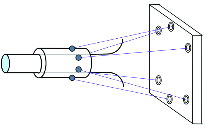
For the minimal model we do not need to make any assumption about the molecular constituents and their spatial organization in the coupler. The only postulates are as follows:
Postulate (a): the energy of the system is lowered monotonically with the increasing overlap between the inner surface of the cylindrically shaped coupler and the outer surface of the MT, and the corresponding binding energy is proportional to the projected length of this overlap along the MT axis;
Postulate (b): the rate of depolymerization of a MT is suppressed by external force.

To our knowledge, the postulate (a) is consistent with the scenario envisaged originally by Hill hill85 , except for the fact that the “roughness” of the MT-coupler interface in the Hill model, which is also an integral part of our realistic model (described in the next section), is not captured by the minimal version of our model. The existence of the sleeve was postulated by Hill hill85 long before information on the the molecular structure of MT-kinetochore coupler began to emerge from experiments. The current knowledge on the inventory of the mitotic machinery have identified the plausible candidates that give rise to the effectively sleeve-like coupler. The Dam1 ring (also called DASH) and the Ndc80 complex seem to be the strongest candidates for the components of the coupler westermann07 ; asbury11 ; buttrick11 ; foley13 .

The postulate (b) is supported by the observation of Franck et al. franck07 in their in-vitro experiments that the rate of depolymerization of MT is suppressed by externally applied tension. It has been known from quite some time that the tips of the depolymerizing protofilaments are curled radially outward from the central axis of the cylindrically shaped MT. Based on this fact, Franck et al.franck07 speculated that the Dam1 ring complex may transmit the external tension to the curled tips of the protofilaments thereby tending to straighten them. Such straightening of the protofilaments is likely to suppress the tendency of the protofilaments to peel away from the depolymerizing tip of the MT. It is worth emphasizing that our results presented here require only the validity of the postulates (a) and (b) irrespective of the nature of the underlying cause of their validity.

II.1 Continuum formulation of the minimal model

The length of the “coupler”is denoted by $L$. In the continuum formulation of the stochastic kinetics, the time-dependent variable $x(t)$ denotes the instantaneous length of overlap between the outer surface of the MT and inner surface of the coaxial cylindrical coupler. Thus, $x=0$ and $x=L$ corresponds to minimum and maximum overlap, respectively; the MT is just on the verge of exiting the coupler when $x=0$.

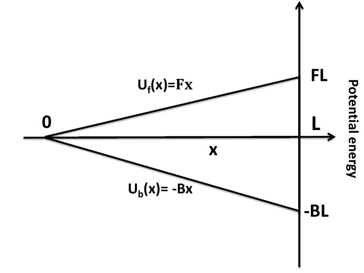
Guided by our postulate (a), in the minimal version of our model we capture the MT-coupler interaction by a potential energy that is proportional to the overlap $x$, i.e.,

$$U_{b}(x)=-Bx.$$ (1)

parametrized by $BL$, the depth of the potential at $x=L$. The form of this interaction in the more realistic version of our model is given in section IV.

Similarly if the MT is pulled outward away from the coupler by a constant external force $F$ (also referred to as a load tension), then this force can be derived from the corresponding potential,

$$U_{f}(x)=Fx$$ (2)

$U_{b}(x)$ and $U_{f}(x)$ are plotted in fig. (2). Net potential felt by the kinetochore is

$$U(x)=U_{b}(x)+U_{f}(x).$$ (3)

Figure 2: Hypothesized potential $U_{b}(x)$ and $U_{f}(x)$ are plotted against the instantaneous length of overlap $x(t)$ between the outer surface of the MT and inner surface of the coaxial cylindrical coupler.

We use the symbols $\alpha$ and $\beta$ to denote the addition and removal rates of the tubulin subunit from the MT. When subjected to a load tension, according to our postulate (b), the depolymerization rate $\beta(F)$ of the MT decreases with increasing strength of the tension $F$ franck07 . More specifically, we assume an exponential decrease of $\beta(F)$ such that

$$\beta(F)=\beta_{\text{max}}~{}e^{-F/F_{*}}$$ (4)

where $\beta_{\text{max}}\equiv\beta(0)$ is the depolymerization rate in the absence of any external force and $F_{*}$ is the characteristic load force at which the MT depolymerization rate is an exponentially small fraction of (i.e., a factor of $1/e$ smaller than) $\beta_{\text{max}}$. Our motivation for assuming the specific exponential form (4) and the key role of the characteristic force $F_{*}$ will be discussed later in this paper.

Stochastic movement of the system can be described by a hypothetical diffusing particle in an external potential U(x). The drift caused by the addition and removal of the tubulin from MT give rise to an additional term $(\alpha-\beta)\ell$ to the drift velocity. Note that the position of the hypothetical particle (i.e., the overlap $x$) can change by any of the following processes:
(i) Even in the absence of any external force, the MT has a natural tendency to approach $x=L$ because the system can lower its energy by increasing the overlap between the outer surface of the MT and the inner surface of the coupler. In other words, the potential $U_{b}(x)$ gives rise an effective force that spontaneously pulls the MT into the coupler.
(ii) The external load tension can pull the MT outward with respect to the coupler thereby decreasing the overlap $x$. Alternatively, an external force can push the MT into the coupler as long as $x$ remains non-zero.
(iii) The overlap $x$ can decrease, as long as it is non-zero, because of the depolymerization of the MT.
(iv) The overlap $x$ can increase because of the polymerization of MT.
(v) Finally, even in the absence of polymerization or depolymerization and force-induced movements, the position $x$ can change because of its one-dimensional diffusion; $D$ being the corresponding diffusion constant.

Therefore, in the overdamped limit,

$$\frac{dx}{dt}=-\frac{1}{\Gamma}\frac{dU(x)}{dx}+(\alpha-\beta)\ell+\frac{\eta(t)}{\Gamma}$$ (5)

where $\Gamma$ is the phenomenological coefficient of the viscous drag and $\eta(t)$ is a Gaussian white noise.

Let $P(x,t)$ denote the probability of finding the overlap $x$ at time $t$. The Fokker Planck equation balakrishanan ,

$$\frac{\partial P(x,t)}{\partial t}=D\frac{\partial^{2}P(x,t)}{\partial x^{2}}-c\frac{\partial P(x,t)}{\partial x},$$ (6)

that corresponds to the stochastic differential equation (5), is essentially a diffusion equation with an additional drift term where the time-independent, but tension-dependent, net drift velocity is

$$c=\underbrace{\frac{B-F}{\Gamma}}_{\text{drift due to two forces}}+\underbrace{(\alpha-\beta_{\text{max}}~{}e^{-F/F_{*}})\ell}_{\text{drift due to polymerization kinetics}}$$ (7)

and D is the diffusion constant. The interplay of the four key components are shown clearly in eqn.(7). The external load tension $F$ competes against $B$ while MT depolymerization competes against polymerization. The load tension $F$ has two mutually opposite effects on the kinetics: (i) it directly tends to decrease $x$ by pulling out the MT from the coupler, and (ii) it indirectly assists increase of $x$ by suppressing $\beta(F)$ that competes against $\alpha$.

The equation (6) can also be written as an equation of continuity

$$\frac{\partial P(x,t)}{\partial t}+\frac{\partial J(x,t)}{\partial x}=0$$ (8)

for the probability density $P(x,t)$, with the probability current density

$$J(x,t)=-D\biggl{[}\frac{\partial P(x,t)}{\partial x}-\frac{cP(x,t)}{D}\biggr{]}$$ (9)

The expression (9) is useful for calculations reported in the sections below.

II.2 Results for the continuum version of the minimal model

The specific initial condition and the boundary conditions that we impose are motivated by the physical situation that our models are intended to capture. If initial value of $x$ is $x_{0}$, the corresponding initial condition for (6) can be expressed as

$$P(x,0)=\delta(x-x_{0})$$ (10)

Throughout this paper we choose $x_{0}=L$, i.e., maximum overlap between the outer surface of the MT and innser surface of the coaxial cylindrical sleeve-like coupler. The lifetime of an arbitrary kt-MT attachment is defined here as the time $t(L)$ taken by the hypothetical particle, that is initially at $x=L$, to reach $x=0$ for the first time. Thus, $t(L)$ is essentially a first passage time redner that fluctuates from one attachment to another. The average value $\langle t(L)\rangle$ is the mean life time of the attachment.

Although $x_{0}=L$ initially, $x$ does not necessarily decrease monotonically. At any arbitrary instant of time $x$ can also increase, just as it can decrease, following the dynamical equations provided $0<x<L$. One advantage of the unique initial condition $x_{0}=L$ is that the random variation of the lifetime of the kt-MT attachment from one run to another arises strictly from the intrinsically random kinetics and not from the choice of any random initial condition. The distribution of the lifetimes of kt-MT coupler that we have derived does not require any further averaging. In contrast, if a random starting location were selected, one extra averaging (over sufficiently large number of random initial locations) would be required to get a meaningful distribution of the lifetimes.

Since the MT is not allowed to penetrate the kinetochore plate, and the length of the sleeve-like coupler is $L$, the overlap $x$ cannot be large than $L$. Therefore, at $x=L$ we impose a reflecting boundary condition

$$J(x,t)|_{(x=L)}=0$$ (11)

which implies

$$\left.\biggl{(}\frac{\partial P(x,t)}{\partial x}-\frac{c}{D}P(x,t)\biggr{)}\right|_{(x=L)}=0$$ (12)

An absorbing boundary condition

$$P(0,t)=0~{}{\rm at}~{}x=0$$ (13)

is imposed so that spontaneous re-formation of the kt-MT is not possible and the time taken for $x$ to attain this boundary, starting from its initial value $x_{0}=L$ is the first-passage time that we define as the life time of the attachment.

(a)

(b)

Figure 3: Mean life time of the kt-MT attachment is plotted against the external force $F$, for a few different values of $F_{*}$, (in (a)), and $B$ (in (b)) . The parameter values used for this plot are $\alpha=30$s^-1, $\beta_{\text{max}}=350$s^-1.

We use the Laplace inversion method balakrishanan for extracting the relevant quantitative information from equation (6). Defining the Laplace transform of probability density by,

$$Q(x,s)=\int_{0}^{\infty}P(x,t)e^{-st}dt$$ (14)

equation (6) can be re-expressed in terms of $Q(x,s)$; solving that equation under the given boundary conditions (see appendix A for the details) we get the exact analytical expression for $Q(x,s)$.

Let $q(x,s|x_{0})$ denote the probability density, in the Laplace space $s$, for the first passage times to reach the position $x$, given that the initial position was $x_{0}$. Using the relation balakrishanan

$$q(0,s|x_{0})=\frac{Q(x_{1},s|x_{0})}{Q(x_{1},s|0)}$$ (15)

between $Q(x,s)$ and $q(x,s|x_{0})$, and the initial condition $x_{0}=L$, we get

$$q(0,s|L)=\frac{V\ \exp\biggl{(}-\frac{cL}{2D}\biggr{)}}{\biggl{[}V\ \cosh\biggl{(}\frac{VL}{2D}\biggr{)}-c\ \sinh\biggl{(}\frac{VL}{2D}\biggr{)}\biggr{]}}$$ (16)

where

$$V=\sqrt{c^{2}+u^{2}}.$$ (17)

includes contributions from both the drift velocity $c$ and the velocity-like quantity

$$u=\sqrt{4sD}$$ (18)

that arises from diffusion.

For the calculation of the mean we do not need the distribution in $t$-space. Instead these can be derived from the relation

$$\langle t\rangle=-\left.\frac{dq(0,s|L)}{ds}\right|_{s=0}$$ (19)

Using the expression (16) for $q(0,s|L)$, we get

$$\langle t\rangle=\frac{D}{c^{2}}\biggl{(}e^{cL/D}-1\biggr{)}-\frac{L}{c}$$ (20)

An interesting feature of eqn.(20) is that $cL$ is like an effective energy barrier; kt-MT detachment is achieved by crossing this barrier. Since in addition to the energetic contributions from $B$ and $F$, the barrier $cL$ gets contribution also from $\alpha$ and $\beta$, this effective barrier is, at least partly, of kinetic origin.

External tension $F$ influences the kt-MT attachment time $\langle t\rangle$ in two possible ways.
(1) $F$ decreases the depth of the linear potential well which effectively reduces the mean attachment time. (2) The same $F$ also reduces the depolymerization rate $\beta(F)$ thereby increasing the mean attachment time.
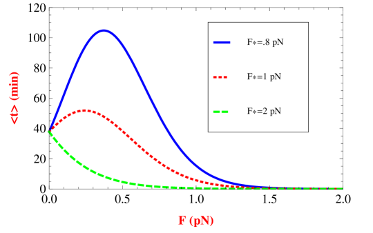
These two effects of the same load tension $F$ act against each other. The second effect can dominate over the first at small $F$, thereby giving rise to nonmonotonic variation of $\langle t\rangle$ with $F$, provided $\beta(F)$ falls sharply with increasing $F$; such a possibility is ensured if $F_{*}$ is sufficiently small. Therefore, as shown graphically in fig.3(a), $\langle t\rangle$ varies nonmonotonically with $F$ for both $F_{*}=0.8$pN and $F_{*}=1.0$pN. But, for $F_{*}=2.0$pN, the fall of $\beta(F)$ is not sharp enough to compensate the reduction of the mean attachment time caused directly by $F$. 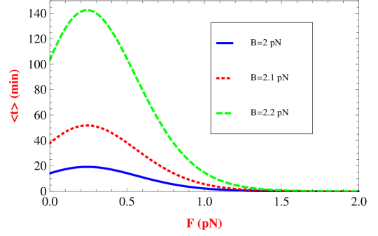Thus, the physical origin of the nonmonotonic variation of $\langle t\rangle$ with $F$ is explained by fig.3(a) in a transparent manner. The nonmonotonic variation of $\langle t\rangle$ with $F$ is displayed also for all the three different values of the parameter $B$ in fig.3(b); for any given $F$, the larger is the $B$ (i.e., the deeper is the potential well), the longer is the mean life time of the kt-MT attachment.

Using the symbol $F_{max}$ to denote the tension that corresponds to the maximum of the average lifetime, from (20) we get

$$F_{max}=F_{*}\log_{e}\biggl{(}\dfrac{k_{B}T\beta\ell}{DF*}\biggr{)}$$ (21)

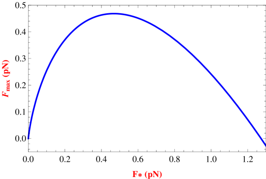
The dependence of $F_{max}$ on $F_{*}$, obtained from (21), is shown in fig.4. Interestingly, the variation of $F_{max}$ with $F_{*}$ is non-monotonic. In the limit $F_{*}\to 0$, $\beta(F)\to 0$ for all $F\neq 0$. On the other hand, as $F_{*}\to\infty$, $\beta\to\beta_{max}$ for all finite $F$. Therefore, in both these limits, $F$-dependence of $\beta$ drops out and kt-MT attachment behaves like a slip-bond. The monotonic decrease of $F_{max}$ with $F_{*}$ in fig.3 arises from the fact that we have not plotted $\langle t\rangle$ for even smaller values of $F_{*}$ where $F_{*}$ increases with $F_{*}$ because the corresponding values of $\langle t\rangle$ turned out to be unphysically long.

Figure 4: Variation of $F_{max}$, the tension that corresponds to the maximum if $\langle t\rangle$, is plotted against $F_{*}$.

At this stage we can scrutinize the necessity of the exponential form (4) for the tension-dependence of the MT depolymerization rate $\beta$. As shown in fig.3(a), a catch-bond-like behavior follows if $\beta(F)$ decreases sufficiently sharply with increasing $F$. On the other hand, if $\beta(F)$ falls very slowly with increasing $F$ the system exhibits a slip-bond-like behavior. The exponential decrease assumed in equation (4) is an ideal choice for the $F$-dependence of $\beta(F)$ because the crossover from catch-bond to slip-bond can be displayed by simply varying $F_{*}$ which determines the sharpness of the decrease $\beta(F)$.

The series representation of equation (20)

$$\langle t\rangle=\biggl{(}\frac{L^{2}}{2D}\biggr{)}\biggl{[}1+2\sum_{n+1}^{\infty}\frac{1}{(n+2)!}\biggl{(}\frac{cL}{D}\biggr{)}^{n}\biggr{]}$$ (22)

is exact. In the special case $B-F=0,\alpha-\beta=0$ eqn.(22) reduces to $\langle t\rangle=L^{2}/(2D)$ which, as expected, arises from kt-MT detachment caused by pure diffusion. The corrections to the diffusive result in the limit $cL/D<<1$, can be estimated from eqn.(22).

As we clearly stated in the introduction, the aim of the minimal model (and, to some extent, even the more detailed model) is not quantitative comparison with the experimental data reported by Akiyoshi et al. Instead, our aim is to present analytical calculations for a minimal model that provides physical insight into the interplay of opposing forces and competing kinetic processes that, together, determine the stability of the kt-MT coupler. Nevertheless, for graphical plots, which often provide a more intuitive understanding, one needs numerical values of the parameters. The largest strength of the load tension applied by Akiyoshi et al. akiyoshi10 was about $13$ pN while the lifetime peaked closed to $4$pN. The longest life time that they measured was about $50$ minutes.

Although the mean lifetimes plotted in fig.3(a) are comparable to the measured values for at least one set of parameter values (corresponding to $F_{*}=1$pN), the numerical values of the corresponding load tension $F$ are much smaller than those applied in the experiment of Akiyoshi et al. akiyoshi10 . However, this discrepancy does not invalidate our theory. The magnitudes of the forces in our model depend on the numerical values of the parameters like, for example, $B$, $\beta(0)$, etc. On the other hand, the corresponding effective values in the experiments of Akiyoshi et al.akiyoshi10 are not known. Therefore, in our plots we have used parameter values that yield lifetimes comparable to those reported in experiments. Most probably, our minimal model does not capture all the details of the in-vitro study akiyoshi10 . Even so, we note that the inclusion of our two postulates is sufficient to generate non-monotonic variation of the lifetimes with load tension.

III The minimal model: discrete formulation and results

We begin by pointing out that in the continuum formulation treated above, the expression (9) for the probability current density $J(x,t)$ can be recast as

$$J(x,t)=-D\biggl{(}\frac{\tilde{U}^{\prime}}{k_{B}T}P+\frac{\partial P}{\partial x}\biggr{)}$$ (23)

with $\tilde{U}^{\prime}(x)=d\tilde{U}/dx$ where the effective potential $\tilde{U}$ is given by

$$\frac{\tilde{U}(x)}{k_{B}T}=\biggl{[}\frac{(F-B)}{k_{B}T}+\ell\frac{\beta-\alpha}{D}\biggr{]}x.$$ (24)

Note that $\tilde{U}(x)$ accounts for the drift caused by the force $B-F$ as well as that arising from the polymerization-depolymerization kinetics of the MT.

In this section, we utilize the effective potential $\tilde{U}(x)$ to simulate the stochastic movements of kinetochore by using a method of discretization popularized by Wang, Peskin and Elston (from now onwards referred to as WPE method) wang03 ; wang07 .

III.1 Discrete formulation of the minimal model

Following WPE prescription, we discretized the space into $M$ cells, each of length $h=L/M$; however, $h$ need not be identical to $\ell$, the separation between the two consecutive binding site of a MT (see fig.5). Accordingly, the continuous effective potential $\tilde{U}(x)$ is replaced by its discrete counterpart

$$\frac{\tilde{U}_{j}}{k_{B}T}=\biggl{[}\frac{(F-B)}{k_{B}T}+\ell\frac{\beta-\alpha}{D}\biggr{]}x_{j}$$ (25)

where $x_{j}$ denotes the position of the center of the $j$-th cell.

Figure 5: The continuous one-dimensional space of length $L$ is discretized into $M$ cells each of length $h=L/M$ following the WPE prescription (see text for details).

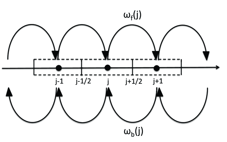
Next we approximate the continuous movement described by the Fokker-Planck equation (6) by a master equation in terms of discrete jumps from the center of one cell to that of an adjacent cell either in the forward or backward direction. In this case the expressions for the forward and backward transition rates $\omega_{f}(j)$ and $\omega_{b}(j)$ (see fig.5) are given by wang03

$$\omega_{f}(j) = \frac{D}{h^{2}}\frac{-\frac{\delta\tilde{U}_{j}}{k_{B}T}}{\exp\biggl{(}-\frac{\delta\tilde{U}_{j}}{k_{B}T}\biggr{)}-1}=\dfrac{1}{h}\dfrac{\dfrac{B-F}{\Gamma}+\ell(\alpha-\beta)}{\exp\biggl{(}-\dfrac{\delta\tilde{U_{j}}}{k_{B}T}\biggr{)}-1}$$ (26)

$$\omega_{b}(j) = \frac{D}{h^{2}}\frac{\frac{\delta\tilde{U}_{j}}{k_{B}T}}{\exp\biggl{(}\frac{\delta\tilde{U}_{j}}{k_{B}T}\biggr{)}-1}=\dfrac{1}{h}\dfrac{\dfrac{F-B}{\Gamma}+\ell(\beta-\alpha)}{\exp\biggl{(}\dfrac{\delta\tilde{U_{j}}}{k_{B}T}\biggr{)}-1}$$ (27)

where

$$\delta\tilde{U}_{j}=\tilde{U}_{j+1}-\tilde{U}_{j}$$ (28)

For the simple potential (25), $\omega_{f}(j)$ and $\omega_{b}(j)$ are independent of site index $j$.

Figure 6: Probability density (histogram) of the distribution of lifetimes of the kt-MT attachments obtained from direct simulation of the discrete version of our minimal model is plotted for a few different values of external tension $F$. The same Laplace-transformed distributions are plotted in the corresponding insets by discrete symbols ($\circ$). Our theoretically predicted distributions in Laplace space for each of the three values of $F$, obtained from the analytical expression (16), are also shown by the continuous lines in the corresponding insets. The numerical values used in this figure for the parameters are: $\alpha=30$s^-1, $\beta_{\text{max}}=350$s^-1, $B=2.1$pN, $F_{*}=1$pN, $L=50$nm $D=700$nm²/s^-1.

III.2 Results for the discrete version of the minimal model

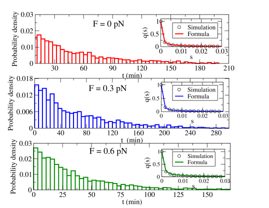
In computer simulations, the MT is fully inserted into the sleeve in the initial state. The simulation produce the numerical data for the first passage time of the MT tip to exit the coupler. In fig. 6, histograms of these numerical data are plotted for a few values of force $F$. Laplace transform of these distributions are compared in the insets with the corresponding prediction of the exact analytical formula (16). Excellent agreement between the theoretical prediction and the simulation data (albeit in the Laplace space) demonstrates how the theory may be useful in analyzing also the distribution of experimentally measured lifetimes of kt-MT attachments in-vitro.

IV Beyond the minimal model: effects of friction in the absence of motor proteins

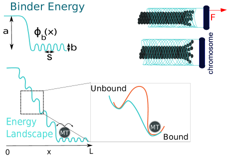
In this section we begin with the assumption that the inner surface of the cylindrically shaped coupler consists of only passive binders. We assume that each binder head engages with the MT by obeying a unit energy function $\phi_{b}(x)$ (see fig.7), which has two key parameters: $a$ measures free energy drop due to binder affinity for the MT lattice, and $b$ describes the activation barrier for transitions between specific MT lattice binding sites shtylla11 . In other words, $a$ is a measure of the strength of the MT-binder affinity while $b$ is a measure of the “roughness” or friction of the MT-coupler interface. The total potential energy function is given by (see fig.7)

$$\Psi_{b}(x)=\sum_{n=0}^{N_{b}-1}\phi_{b}(x-ns)$$ (29)

where $s$ is the spacing between consecutive coupler binders (see Fig 7). Binder spacing is an arbitrary parameter. Here we set $s=\ell$, where $\ell$ is the distance between consecutive MT binding sites.

Figure 7: The theoretical model, extended by incorporating a realistic kt-MT interaction potential, is depicted schematically (see text for the details of $\psi_{b}(x)$ and $\Psi_{b}(x)$). The load tension $F$ tilts the potential energy landscape $\Psi_{b}(x)$. The tension-dependent depolymerization rate $\beta(F)$ increases the effective barrier along the unbinding pathway (orange line, inset) by slowing down depolymerization.

Figure 8: Mean attachment time for the model depicted in fig.7 plotted for three different regimes of parameters. Low-friction regime (blue line) is obtained from eq. (20) with a = 0.5k_BT, b = 0.001a. Intermediate regime (circle) a = 0.5k_BT, b = 0.04a, and intermediate regime (square) a = 0.6k_BT, b = 0.2a. High-friction regime (dashed red line) is obtained from eq. (32) with $\beta_{max}=300$, $\alpha=0$, $F^{*}=0.6$ pN.

For $\Psi_{b}(x)$ in our numerical calculations, we have used the simple expression

$$\Psi_{b}(x) =\begin{cases}f(x)\left(1-\cos(\frac{2\pi x}{\ell})\right)+h(x)&x\leq N_{b}{\ell}\\ f(N_{1}\ell)\left(1-\cos(\frac{2\pi x}{\ell})\right)+h(N_{b}\ell)&x>N_{b}{\ell}.\end{cases}$$ (30)

where $f(x)=\dfrac{a}{2\ell}\left(\frac{b}{a}x+C\right)$, $C=0.172$ and $h(x)=-\dfrac{ax}{\ell}$. The linear and scalar coefficients in eq. (30) arise because we use a Fourier series to approximate the well function expression. Thus, the MT-coupler interaction is represented more realistically by $\Psi_{b}(x)$ than by $U_{b}(x)$ of the minimal model. The friction arising from the potential landscape $\Psi_{b}(x)$ gives rise to a jump-drift-diffusion process. As we’ll point out below, this general version of our model reduces to the minimal version discussed above, and hence effectively to a drift-diffusion process, in a special limiting case.

In infinitesimal time interval $dt$, the change $dx$ of the overlap is given by

$$dx(t)=\frac{1}{\Gamma}\left[-\Psi_{b}^{\prime}(x)-F\right]dt+\ell dN_{r}(t)+\sigma dW(t)$$ (31)

where, as before, the constant $F$ is the external load tension and $\Gamma$ is the effective drag coefficient. $dW(t)$ accounts for the thermal diffusion of the coupler on the lattice with $\sigma=\sqrt{2k_{B}T/\Gamma}$, and $N_{r}(t)$ is a Poisson counting process describing the MT tip dynamics with rate $r=\alpha-\beta$ that is decided by the difference of the MT polymerization rate $\alpha$ and MT depolymerization rate $\beta$. The stochastic differential equation (31) is essentially equivalent to the Langevin equation (5); the form (31) is used in our numerical computations for the convenience of implementation.

$N_{b}$ is characteristic of the structure of the coupler (coupler length) whereas its energetics depend on $\Psi_{b}$ (i.e., on the parameters $a$, $b$) and $F$; the stochastic kinetics are influenced by the interplay of forces arising from the potential landscape, random Brownian forces, and by $\alpha$, $\beta$. By a combination of standard analytical and numerical methods, we study the trends of variation of $\langle t(L)\rangle$ with (a) $F$, as well as, the (b) size, (c) energetics, and (d) kinetics of the coupler.

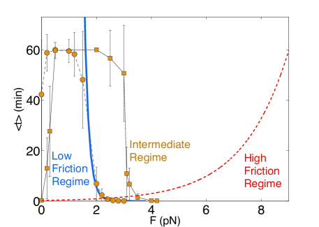
It is difficult to derive an exact analytical expression for the mean first passage time corresponding to eq. (31) that would be valid in all parameter regimes. Therefore, we explore two limiting cases for which explicit approximate solutions can be obtained: (a) Low-friction regime ($b<<k_{B}T$), and (b) High-friction regime ($b>>k_{B}T$). In the low-friction regime the coupler can easily rearrange its position relative to the MT; in this regime $\langle t(L)\rangle$ approximated well by the expression in equation (20) In the high-friction regime large $b$ leads to strong local pinning that practically stalls it. The only mode available for detachment of the coupler is via depolymerization of the MT. Consequently, in this regime

$$\langle t(L)\rangle\approx\biggl{(}\frac{L}{\ell\beta_{\text{max}}}\biggr{)}~{}e^{F/F_{*}}.$$ (32)

The exponential increase of $\langle t(L)\rangle$ with $F$ in the high-friction regime can be regarded as an artifact of the unphysical (or, unrealizable) nature of this regime.

Unless explicitly stated otherwise, the parameter values that we have used for our numerical calculations in this section are given in the table IV.

Parameter Description	Symbol	Values Tested
MT binding site spacing	$\ell$	8/13 nm hill85 ; joglekar02 ; shtylla11
Maximal coupler length	$L$	50 nm joglekar06 ; Gonen2012 ; Joglekar2008 ; Johnston2010
Maximal number of coupler binders	$N_{b}$	15-65 Powers2009 ; Johnston2010
Polymerization Rate	$\alpha$	$20-50$ $s^{-1}$joglekar02 ; hill85 ; Waters1996 ; shtylla11
Maximal Depolymerization Rate	$\beta_{\text{max}}$	$100-350$ $s^{-1}$ hill85 ; Waters1996 ; shtylla11
Critical Depolymerization Force	$F_{*}$	$0.3-5$ pN (estimated here)
External load Force	$F$	$0-5$ pN
Force of attractive kt-MT interaction	$B$	$2-2.5$ pN
MT lattice/binder binding energy	$a$	$0.4k_{B}T-3k_{B}T$ hill85 ; joglekar02 ; Powers2009 ; shtylla11
Binder activation barrier	$b$	$0.001a-0.4a$ (estimated here)
Diffusion constant	$D$	$700$ nm2s-1 hill85 ; joglekar02 ; shtylla11
Effective drag coefficient	$\Gamma$	$6$ pNs$\mu$m-1hill85 ; Marshall2001 ; joglekar02 ; shtylla11

Figure 9: Results of simulations for the model depicted in fig.7, using equation (31) and $F^{*}=1/3$. (a)-(b) $\langle t(L)\rangle$ for two sets of maximal rates of MT depolymerization with the ratio $\beta_{max}/\alpha$ fixed. In (a) the data are obtained for an intermediate regime coupler, with $a=0.45$ k_BT, $b=0.04a,N_{b}=45$, and in (b) for a shorter coupler in the low-friction regime with $a=0.4$ k_BT , $b=0.001a,N_{b}=32$. (c)-(d) $\langle t(L)\rangle$ for intermediate regime couplers. In (c) are shown data with two different strengths of friction caused by two values of $b$, and in (d) for two different binding energies given by $a$. The MT rates are $\beta_{max}=350$ s^-1, $\alpha=50$ s^-1 for (c)-(d). (e) $\langle t(L)\rangle$ plotted against $F$ for three different lengths of the low-friction coupler from (a) with $a=0.4$ k_BT , $b=0.001a$, $\beta_{max}=140$ s^-1, $\alpha=20$ s^-1. Error bars mark standard deviation.

Figure 10: Force-speed relations obtained by direct numerical simulation of the model depicted in fig.7, using the corresponding dynamical equation (31) and $F^{*}=1/3$, is plotted in the low-friction regime and the corresponding data for the intermediate regime. The parameters are $N_{b}$ = 65, a = 0.45 k_BT, $\beta_{max}=140$ s^-1, $\alpha=20$ s^-1. Error bars mark standard deviation.

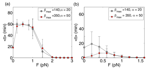
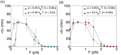
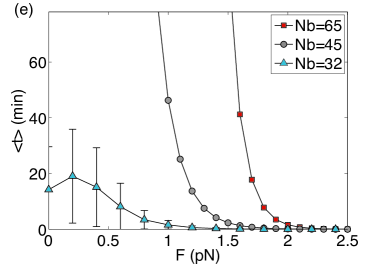
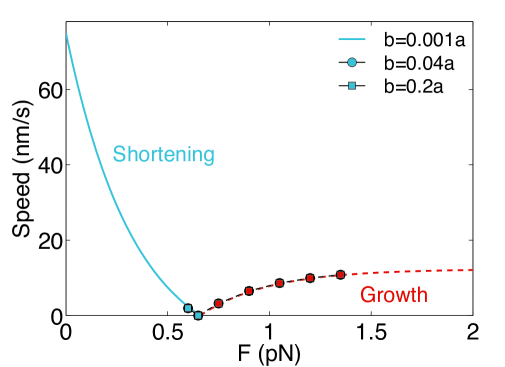
For numerical simulations of this version of our model in the intermediate regime we used the parameter values which are within the range reported in the literaturejoglekar09 ; wan09 ; lawrimore11 . Consequently, computed $\langle t(L)\rangle$ turn out to be comparable to those observed in the experiments. Some of the typical curves are plotted in Figs.9.

$\bullet$ Effects of variation of rate of kinetics

The effects of varying the maximal rate of depolymerization $\beta_{\text{max}}$, keeping the ratio $\beta_{\text{max}}/\alpha$ fixed, is demonstrated in figs.9(a) and (b). Clearly, in such situations, the kt-MT attachment can exhibit catch-bond-like or slip-bond-like behavior depending on the value of $\beta_{\text{max}}$.

$\bullet$ Effects of variation of parameters that characterize energetics

The effects of the energetics, namely the influences of the parameters $a$ and $b$ that determine the potential energy landscape, are displayed in figs.9(c) and (d). The effects of varying the number of binders $N_{b}$ is shown in fig.9(e). In all these cases the nonmonotonic variation of $\langle t(L)\rangle$ with $F$ seems to be a generic feature, except that $\langle t(L)\rangle$ may become too large to be observable for some values of the parameters (see, for example, fig.9(e).

$\bullet$ Tension-induced switching from depolymerization to polymerization

Fig.10 shows the key role of the external tension $F$ in deciding the direction of the velocity. Suppose the parameter values are chosen such that $\beta_{\text{max}}$ dominates over $\alpha$ in the absence of external tension thereby ensuring depolymerization of the MT. When the external tension is applied, the depolymerization is suppressed. Increasing $F$ can eventually cause such strong suppression of the depolymerization that, beyond a certain strength of $F$, $\alpha$ dominates over $\beta(F)$. In such a scenario, the MT switches from the depolymerization mode to polymerization mode at a threshold strength of $F$.

V Summary and Conclusions

In this paper, we have presented theoretical models of kt-MT attachment at three levels of detail starting with a minimal version that captures only the key components and essential processes. These models mimic kt-MT attachments reconstituted in-vitro from purified components extracted from budding yeast akiyoshi10 .

Exploiting the simplicity of the minimal version of the model, we have calculated the distribution of the lifetimes of the kt-MT attachments analytically and compared the results with the corresponding simulation data. Equation (16) encapsulates the main result of this part of the manuscript. The strength of the minimal model is that the results can be derived analytically. In spite of its simplicity, this minimal model provides deep insight into the roles of opposing forces and competing kinetics in the tension-dependence of the life time of the kt-MT attachments.

The second version of the model is an extension of the minimal model; it incorporates some more realistic features of the interaction between the MT and the coupler. For the second model we have succeeded in calculating analytically only the mean lifetime of the kt-MT attachments under reasonable schemes of approximation.

The analytical expression (20) for the mean life time of the kt-MT attachment in the minimal model has been derived from the corresponding full distribution (16) of the life times, The nonmonotonic variation of the mean lifetime of the kt-MT attachments with external tension exhibited over wide range of values of the model parameters in both the models is consistent with the similar trend observed in the in-vitro experiments akiyoshi10 . The realistic potential landscape in the second model does not alter this qualitative trend. We have also demonstrated that the nonmonotonicity of the variation of $\langle t\rangle$ with $F$ depends on the rapidity of decrease of $\beta(F)$ with increasing $F$. By varying $F_{*}$, which determines the sharpness of the decrease of $\beta(F)$, we have shown how the catch-bond-like behavior crosses over to a slip-bond-like behavior. Moreover, our analytical calculations also show that, unlike other conventional catch-bonds, the catch-bond-like behavior of the kt-MT attachment arises from the interplay of not only forces derivable from the potential landscape, but also by a competition of the kinetics of polymerization and depolymerization of the MT. In fact, the barrier against the breakdown of the attachment gets contributions from both opposing forces and competing kinetic processes. The slip-bond-like monotonic decrease of $\langle t(L)\rangle$ with $F$ observed in some of the parameter regimes (whose physical origin has been explained in terms of the nature of $F$-dependence of the depolymerization rate $\beta(F)$), might be detectable in experiments under conditions different from those used by Akiyoshi et al.akiyoshi10 .

As expected, we have found that the molecular motors enhance stability or tend to destabilize the kt-MT attachment depending on whether the force it generates opposes or assists the external tension. The latter awaits experimental confirmation. Moreover, our analytical predictions on the distribution of the lifetimes will be useful in the future in analyzing the statistical properties of the lifetimes provided the in-vitro experiment on the reconstituted kt-MT attachment is repeated sufficiently large number of times.

In principle, the models presented here can be further extended by including active force generators like molecular motors chowdhury13a ; chowdhury13b . However, so far such active force generators have not been detected at the kt-MT interface in budding yeast although such force-generating motors have been found in other cells including, for example, mammalian cells. But, in contrast to budding yeast, where each kinetochore can attach to only one MT, multiple MTs can attach with each kinetochore in a mammalian cell. Since modeling of kt-MT attachment in this paper is focussed almost exclusively on budding yeast, we have not discussed the effects of molecular motors in the main text. Thus, the extended model in appendix B is not a complete model of kt-MT attachment in mammalian cells; it is intended to indicate how the effects of molecular motors can be incorporated within the broad theoretical framework developed in this paper. In near future we hope to extend our model to kt-MT attachments in mammalian cells. However, at present, the main hurdle in this modeling is the lack of our current understanding as to how multiple MTs attached to the same kt coordinate their kinetics mcintosh12 .

V.1 Comparison with earlier kinetic model of kt-MT attachments

The “sleeve model” developed originally by Hill hill85 was adapted by Joglekar and Hunt joglekar02 , to account for the phenomenon of “directional instability” skibbens93 ; cassimeris94 (also referred to as chromosome oscillation) observed during mitosis in vertebrates. In those cells each kt can attach with several MT (typically, up to 35) and this feature was also incorporated in the model studied by Joglekar and Hunt by carrying out computer simulations.

Our work differs significantly from that of Joglekar and Hunt joglekar02 . First, our model is intended to account for the qualititative features of the results obtained from a much simpler in-vitro system where only one MT is attached to only a single kt that is subjected to an externally applied load force that, in our model, is assumed to alter the rate of MT depolymerization itself. Moreover, because of their motivation in studying directional instability, Joglekar and Hunt joglekar02 put major emphasis on monitoring the spatial displacements that characterize this instability. In contrast, the quantity of our main interest is the life time of the kt-MT attachments.

The spatial excursions of the kinetochores was also the main quantity of interest of Gardner et al.gardner05 who studied the effects of tension-mediated regulation of the kinetics of kinetochore MTs by computer simulation of a related model. The scope of the more detailed model studied by Scholey et al.civelekoglu06 was even broader. Our force-balance equations are similar, at least in principle, to the force-balance equations formulated by Scholey et al.civelekoglu06 . However, instead of the spatial displacements of the kinetochores, the lifetimes of the kt-MT attachments are the main focus of our investigation.

Most of the earlier models were based on the assumption that the coupler is a stable sleeve or ring. In recent years, a new class of models have been developed on the basis of an altogether different assumption regarding the nature of the coupler. In this scenario zaytsev13 microtubule associated proteins (MAPs) are assumed to make transient attachments with the MT (i.e., each MAP attaches to the MT for a brief duration before getting detached from it). The entropic contribution to the force is significant and slight variation in the mean lifetime of the individual transient attachments of the MAPs can have large effect on the lifetime of the kt-MT attachment.

In order to account for their experimental observations, Akiyoshi et al. akiyoshi10 developed a 2-state kinetic model. This model was motivated by the formal analogy with the models of ‘catch-bonds’ in other systems. The growing and shrinking states of the MT were argued to be analogs of the strongly- and weakly-bound states in the models of catch-bonds. In their 4-parameter kinetic model, two parameters were the rates of transitions between the states of growth and shrinkage of the MT. The remaining two parameters were the rates of detachment of the kinetochore from the MT while the latter is in the growing and shrinking phases, respectively. Postulating exponential dependence of the type $k_{n}(F)=k_{n}^{0}\exp(F/F_{n})$ for each of the four rate constants (n=1,2,3,4), on the external tension $F$, Akiyoshi et al. extracted the numerical values of the 8 parameters $k_{n}^{0},F_{n}$ (n=1,2,3,4) corresponding to the best fit to their experimental data akiyoshi10 .

In their model, Akiyoshi et al.akiyoshi10 did not explicitly treat the kinetics of the polymerization and depolymerization, by attachment and detachment of the successive subunits (more precisely, the $\alpha-\beta$ tubulin dimers), during the growing and shrinking phases of the MT, respectively. Therefore, the force-dependence of the four rate constants that provide the best fit to their experimental data do not indicate the corresponding force-dependences of the rates of polymerization and depolymerization of the MT. Moreover, the potential energy of interaction between the MT and the coupler as well as the effect of the external tension on this potential energy landscape are not incorporated explicitly in their model. Thus, the model of Akiyoshi et al.akiyoshi10 does not directly demonstrate the interplay of the opposing forces and competing kinetics.

Since neither any structural features of the coupler, nor the nature of its interaction with the MT enters explicitly into Akiyoshi et al.’s akiyoshi10 model, their model cannot be used to study the effects of the size and composition of the coupler or that of the nature of the MT-coupler interaction. Neither can it be used to account for the special features of hybrid couplers. In contrast, in this paper we have used our models to study the effects of varying (i) the size of the coupler, (ii) relative population of active force generators (molecular motors) and passive binders, as well as (iii) the depth and roughness of the potential of interaction between the coupler and the MT.

V.2 Comparison with catch-bond mechanisms in other ligand-receptor systems

Catch bond formed by the fimbriae of E-coli bacteria with target cell surface and that formed by eukaryotic P-selectin and integrin receptors with their ligands have been studied extensively in recent years thomas08a ; thomas08b ; thomas09 ; sokurenko08 ; prezhdo09 ; evans07 ; zhu05 ; zhu08 ; mcever10 ; sundd11 ; sundd13 to understand their mechanism.

In this paper we have focussed exclusively on the kt-MT attachments to understand the mechanism of its catch-bond-like behavior akiyoshi10 using simple theoretical models. One distinct feature of the MT is that, unlike other ligands, these stiff filaments are capable of generating push and pull by their polymerization and depolymerization, respectively. In particular, the pulling force generated by a MT is powered by the hydrolysis of GTP bound to the tubulin subunits. As we have shown in this paper, the competing polymerization and depolymerization of MT gives rise to a unique feature of the catch-bond-like behavior of kt-MT attachments where the stable state can be a non-equilibrium (local) steady state rather than a local minimum of the free energy of the ligand-receptor system. We hope the modeling methodology developed here can be usefully adapted to understand the catch-bond-like behavior of depolymerizing actin under load tension observed recently by carrying out in-vitro experiments with atomic force microscope (AFM) lee13 .

Acknowledgements: DC thanks Frank Jülicher for valuable comments. This work has been supported in part by CSIR (India) through a senior research fellowship (AKS), by NSF through the grant DMS- 1358932 (BS), by MBI, the Ohio State University, through the NSF grant DMS 0931642 (BS and DC), by IIT Kanpur through Dr. Jag Mohan Garg Chair professorship (DC), by SERB (India) through J.C. Bose National Fellowship (DC), by DBT (India) through a research grant (DC), and by the Visitors Program of the Max-Planck Institute for the Physics of Complex Systems, Dresden (DC).

Appendix A Eqn. for $Q(x,s)$ and its solution for the minimal model

From equation (6) we get

$$\frac{d^{2}Q(x,s)}{dx^{2}}-\frac{c}{D}\frac{dQ(x,s)}{dx}-\frac{s}{D}Q(x,s)=-\frac{1}{D}\delta(x-x_{0})$$ (33)

For $x<x_{0}$, equation (33) has following solution.

$$Q(x,s)=A_{1}e^{k_{1}(L-x)}+B_{1}e^{k_{2}(L-x)}$$ (34)

Similarly, for $x>x_{0}$, solution of equation (33) is,

$$Q(x,s)=A_{2}e^{k_{1}(L-x)}+B_{2}e^{k_{2}(L-x)}$$ (35)

where $k_{1}$ and $k_{2}$ are given by

$$k_{1}=\frac{-c-\sqrt{c^{2}+u^{2}}}{2D},~{}\rm~{}~{}k_{2}=\frac{-c+\sqrt{c^{2}+u^{2}}}{2D}$$ (36)

with $u=\sqrt{4sD}$. Imposing the absorbing boundary condition at $x=0$ on $Q(x,s)$ we find

$$B_{1}=-A_{1}e^{(k_{1}-k_{2})L}.$$ (37)

Now $Q(x,s)$ and it’s first derivative must satisfy the following matching conditions at $x=x_{0}$:

$$A_{1}e^{k_{1}(L-x_{0})}+B_{1}e^{k_{2}(L-x_{0})}=A_{2}e^{k_{1}(L-x_{0})}+B_{2}e^{k_{2}(L-x_{0})}$$ (38)

$$\left.\frac{dQ(x,s)}{dx}\right|_{x=x_{0}+0}-\left.\frac{dQ(x,s)}{dx}\right|_{x=x_{0}-0}=-\frac{1}{D}$$ (39)

Reflecting boundary condition at $x=L$ gives,

$$A_{2}\biggl{(}k_{1}+\frac{c}{D}\biggr{)}+B_{2}\biggl{(}k_{2}+\frac{c}{D}\biggr{)}=0$$ (40)

The four unknowns $A_{1}$, $B_{1}$, $A_{2}$ and $B_{2}$ can be obtained by solving the three equations (37)-(40). As we’ll see later, we need $Q(x,s)$ only for $x<x_{0}$. Therefore, we give the expression for $A_{1}$ only in the region $x<x_{0}$:

$$A_{1}=e^{\frac{V(L-x_{0})}{2D}}e^{k_{2}x_{0}}\frac{V\ \cosh\biggl{(}\frac{V(L-x_{0})}{2D}\biggr{)}-c\ \sinh\biggl{(}\frac{V(L-x_{0})}{2D}\biggr{)}}{V(V-c)e^{k_{2}L}+V(V+c)e^{k_{1}L}}$$ (41)

with $V=\sqrt{c^{2}+u^{2}}$. And $B_{1}$ can be find by using equation 37. Thus, for $x<x_{0}$

$$Q(x,s)=A_{1}e^{k_{1}L}[e^{-k_{1}x}-e^{-k_{2}x}]$$ (42)

where the $s$-dependence enters through the $s$-dependence of $u$ (see eqn.(18) that enters into the expression (17) for $V$.

Appendix B Model of “Hybrid” Coupler: effects of molecular motors

So far no motor protein has been detected at the kinetochore in budding yeast, which is the object of our modeling in this paper, But, in most of the eukaryotes (e.g., mammalian cells) such motors have been found in the kinetochores each of which, however, attaches to more than one MT. On the other hand, not more than a single MT can attach to each kt in budding yeat. Nevertheless, we extend our model further by including motor proteins sharp00b ; scholey03b ; salmon04 , which are active force generators, in addition to the passive binders in the model coupler. We hope to extend this hybrid coupler, in near future, by integrating more than one MT to model kt-MT attachments of mammalian cells.

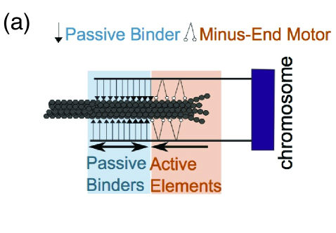
As indicated in recent experiments dumont12 ; gonen12 , the outermost layer of the hybrid coupler in mammalian cells consists of passive binders while the innermost layer, that is adjacent to the kt, is composed of active force generators. In the model of hybrid coupler we represent the active force generators by molecular motors (see Fig 11A). As we show in this section, the nature of the response of the kt-MT attachment to the external tension now depends on whether the motors are plus-end directed (e.g., kinesin) or minus-end directed (e.g., dynein). We use the subscripts or superscripts $+$ and $-$ to refer to the plus-end and minus-end directed motors, respectively.

Following the general trend in the literature on molecular motors civelekoglu06 ; efremov07 . we also postulate a linear force-velocity relation for the individual motors:

$$f_{\pm}=F_{max}^{\pm}\left(1-\frac{v_{\pm}}{V^{\pm}_{max}}\right),$$ (43)

where $F_{max}^{\pm}$ and $V_{max}^{\pm}$ are the stall force and maximal velocity for the plus-end directed and minus-end directed motors, respectively, whereas $v_{\pm}$ are the corresponding instantaneous velocities.

In the dynamical equation for the overlap variable $x$, we now include an additional force that is generated by the motor proteins.

Figure 11: (a) Diagram of a hybrid coupler arrangement. (b) Comparison of $\langle t(L)\rangle$ for an intermediate regime hybrid coupler with ($\eta=0.04$) and without ($\eta=0$) minus-end motors with $N_{b}=45,a=0.45$ k_BT , $b=0.04a$, $\beta_{max}=350$ s^-1, $\alpha=50$ s^-1. (c) Breaking load, F_break for a low-friction hybrid coupler versus motor densities; minus-end motors (squares) and plus-end motors (circles). (d). Average speed vs force for varying densities of minus-end motors. Inset. Stall forces for each motor density fraction. Parameters for (c)-(d) are $N_{b}=52,b=0.01a$, $\beta_{max}=140$ s^-1, $\alpha=20$ s^-1. For all panels $F^{*}=1/3$.

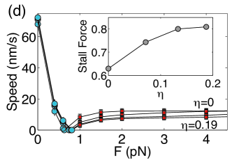
We start with the force balance equation which does not include random fluctuations for the overlap velocity

$$\frac{dx(t)}{dt}-V_{MT}=\frac{1}{\Gamma}\sum F=\frac{1}{\Gamma}\Big{(}-\Psi_{b}^{\prime}(x)-F_{\text{load}}+F_{\text{A}}(x)\Big{)},$$ (44)

where $\Gamma$ is the effective coupler drag coefficient and $V_{MT}$ is the velocity of the MT tip with respect to a space-fixed frame of reference. The active force term

$$F_{\text{A}}(x)=d_{m}(x)(n_{-}f_{-}-n_{+}f_{+})$$ (45)

with the motor density function

$$d_{m}(x) =(x-N_{b}{\ell})(H(x-N_{b}{\ell})-H(x-N_{b}{\ell}-L_{m}))$$ (46)

$$+L_{m}H(x-N_{b}{\ell}-L_{m}),$$ (47)

where $H(x)$ is the standard Heaviside step function and $L_{m}=8$ nm, corresponds to the total horizontal length of the coupler that can be populated by active components (in three-dimensions this corresponds to one layer of motors working around a MT with 13 protofilament tracks, with one motor per track).

Note that in the symbol $f_{\pm}$, the subscript minus (-) / plus (+) denote the force generated by the minus-end / plus-end directed motors that tend to increase / decrease the overlap $x$. We have expression (43) for $f_{\pm}$ where $F_{max}^{\pm}$ and $V_{max}^{\pm}$ are the stall force and maximal velocity for the plus-end directed and minus-end directed motors, respectively, whereas $v_{\pm}$ are the corresponding instantaneous velocities. Next we express $v_{\pm}$ in terms of $dx/dt$. Using $x=x_{tip}-x_{motor}$, in case of minus-end directed motors

$$\frac{dx}{dt} =\frac{dx_{tip}}{dt}-\frac{dx_{motor}}{dt}$$ (48)

$$=V_{MT}+v_{-}$$ (49)

Similarly, if only plus-end-directed motors are present,

$$\frac{dx}{dt} =V_{MT}-v_{+}.$$ (50)

Substituting eqs. (49) and (50) into eq. (44) we get

$$\frac{dx}{dt}=\frac{1}{\Gamma} \Big{[}-\Psi_{b}^{\prime}(x)-F_{\text{load}}+d_{m}(x)\Big{(}n_{-}F_{max}^{-}\left(1-\frac{dx/dt-V_{MT}}{V^{-}_{max}}\right)$$

$$-n_{+}F_{max}^{+}\left(1-\frac{V_{MT}-dx/dt}{V^{+}_{max}}\right)\Big{)}\Big{]}+V_{MT}.$$ (51)

Regrouping the velocity terms we obtain the following equation for coupler overlap,

$$\frac{dx}{dt} =\frac{1}{\Gamma(x)}\left[-\Psi_{b}^{\prime}(x)-F_{\text{load}}+d_{m}(x)(n_{-}F_{max}^{-}-n_{+}F_{max}^{+})\right]+V_{MT}.$$ (52)

where $\Gamma(x)=\Gamma+\mu^{-}(x)+\mu^{+}(x)$ and

$$\mu^{\pm}=d_{m}(x)\biggl{(}\frac{n_{\pm}F^{\pm}_{max}}{V^{\pm}_{max}}\biggr{)}.$$ (53)

The coupler movement described by eq. (52) is fully deterministic. Next, we write down a stochastic differential equation (SDE) that would, upon averaging, correspond to the deterministic equations written above. Suppose over a small time interval $\delta t$ the number of subunits (an $\alpha-\beta$ tubulin dimer) added and removed from the tip of the MT by polymerization and depolymerization are $dN_{r}$, an independent homogenous Poisson process. We capture the effects of random Brownian forces through the noise $W(t)$ which is assumed to be a Gaussian stochastic process, which also includes the effects of fluctuations both in the chemical reactions and mechanical stepping involved in each cycle of the individual motors. Thus, finally, the equation for the hybrid coupler overlap reads

$$dx =\frac{1}{\Gamma(x)}\left[-\Psi_{b}^{\prime}(x)-F_{\text{load}}+d_{m}(x)(n_{-}F_{max}^{-}-n_{+}F_{max}^{+})\right]dt$$

$$+\ell dN_{r}(t)+\sigma dW(t).$$ (54)

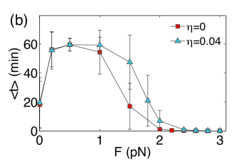
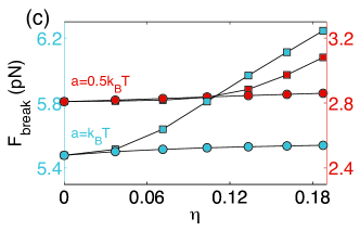
In Fig. 11 we plot results for a hybrid coupler with varying density fractions of motors at the active interface, measured by $\eta=n_{\pm}/(N_{b}+n_{\pm})$. The non-monotonic nature of $\langle t(L)\rangle$ is preserved when the active components are added (see Fig. 11B). If the active force generators are minus-end directed (for example, dyneins), the force exerted by them oppose load force. Consequently, the mean lifetime $\langle t(L)\rangle$ os the kt-MT attachment increases as motor fractions, $\eta$ become larger (see Figs. 11C). For a given $\eta$, the extent of such motor-induced extra stabilization of hybrid couplers can be sensitive to the binding energy of the passive components measured by $a$ (see Fig 11C). Despite enhancing the stability, higher numbers of load opposing motors can also lower the ability of the coupler to efficiently track rescued MT tips, as noted by the slower coupler velocities in Fig. 11D. Plus-end directed motors (for example, CENP-E kinesin), which oppose overlap between the MT and the coupler, generate force that assist the external load. If the active force generators in the hybrid coupler are such plus-end directed motors, neither the coupler velocities and nor the breaking force $F_{\text{break}}$ show significant variation as $\eta$ is varied under a given tension, provided that there are sufficient numbers of passive binder components supporting attachment.

References

- (1) H. Lodish, A. Berk, S L. Zipursky, P. Matsudaira, D. Baltimore, and J. Darnell, Molecular Cell Biology, 4th edition, (W. H. Freeman, 2000).
- (2) I. M. Cheeseman and A. Desai, Nature Rev. Mol. Cell. Biol. 9, 33 (2008).
- (3) E. Karsenti and I. Vernos, Science 294, 543 (2001).
- (4) J.R. McIntosh, M.I. Molodtsov and F.I. Ataullakhanov,
- (5) D. Chowdhury, Phys. Rep. 529, 1 (2013).
- (6) D. Chowdhury, Biophys. J. 104, 2331 (2013).
- (7) G. Civelekoglu-scholey, D.J. Sharp, A. Mogilner and J.M. Scholey, Biophys. J. 90, 3966 (2006).,
- (8) A.P. Joglekar and A.J. Hunt, Biophys. J. 83, 42 (2002).
- (9) M.K. Gardner, C.G. Pearson, B.L. Sprague, T.R. Zarzar, K. Bloom, E.D. Salmon and D.J. Odde, Mol. Biol. Cell 16, 3764 (2005). Quart. Rev. Biophys. 45, 147-207 (2012).
- (10) C.S. Peskin and G.F. Oster, Biophys. J. 69, 2268 (1995).
- (11) B. Akiyoshi, K. K. Sarangapani, A. F. Powers, C. R. Nelson, S. L. Reichow, H. Arellano-Santoyo, T. Gonen, J. A. Ranish, C. L. Asbury and S. Biggins, Nature 468, 576 (2010).
- (12) W. E. Thomas, V. Vogel, and E. Sokurenko, Ann Rev Biophys, 37, 399-416 (2008).
- (13) H. Wang, C. Peskin and T. Elston, J. Theo. Biol. 221, 491 (2003).
- (14) H. Wang, T. C. Elston, J. Stat. Phys. 128, 35 (2007).
- (15) T. Hill, Proc. Natl. Acad. Sci. U.S.A. 82, 4404 (1985).
- (16) S. Westermann, D.G. Drubin and G. Barnes, Annu. Rev. Biochem. 76, 563 (2007).
- (17) C.L. Asbury, J.F. Tien and T.N. Davis, Trends in Cell Biol. 21, 38 (2011).
- (18) G.J. Buttrick and J.B.A. Millar, Chromosome Res. 19, 393 (2011).
- (19) E.A. Foley and T.M. Kapoor, Nat. Rev. Mo. Cell Biol. 14, 25 (2013).
- (20) A. D. Franck, A. F. Powers, D. R. Gestaut, T. Gonen, T. N. Davis, C. L. Asbury, Nat Cell Biol 9, 832 (2007).
- (21) S. Redner, A guide to first-passage processes, (Cambridge University Press, 2001).
- (22) V. Balakrishnan, Elements of nonequilibrium statistical mechanics, (Ane books Pvt. Ltd., 2008)
- (23) B. Shtylla and J. P. Keener, SIAM J. APPL. MATH 71 1821 (2011).
- (24) S. Gonen, B. Akiyoshi, M.G. Iadanza, D. Shi, N. Duggan, S. Biggins, T. Gonen, Nat. Struct. Mol. Biol., 19, 925 (2012).
- (25) A.P. Joglekar, D. Bouck, K. Finley, X. Liu, Y. Wan, J. Berman, X. He, E.D. Salmon and K.S. Bloom, J. Cell Biol., 181, 587 (2008).
- (26) K. Johnston, A. Joglekar, T. Hori, A. Suzuki, T. Fukagawa, and E.D. Salmon, ,J. Cell Biol., 189, 937 (2010).
- (27) A.F. Powers, and A.D. Franck, and D.R. Gestaut, and J. Cooper, B. Gracyzk, R.R. Wei, L. Wordeman, T.N. Davis, C. L.Asbury, Cell, 136, 865 (2009).
- (28) J.C. Waters, T.J. Mitchison, C.L. Rieder and Salmon, ED, Mol. Biol. Cell, 7, 1547 (1996).
- (29) W. F. Marshall, J. F. Marko, D. A. Agard and J. W. Sedat, Curr. Biol. 11, 569 (2001).
- (30) A. P. Joglekar, D. C. Bouck, J. N. Molk, K. S. Bloom and E. D. Salmon, Nat. Cell Biol. 8, 581 (2006).
- (31) A. P. Joglekar, K. Bloom and E. D. Salmon, Curr. Biol. 19, 694 (2009).
- (32) X. Wan, R. P. O’Quinn, H. L. Pierce, A. P. Joglekar, W. E. Gall, J. G. DeLuca, C. W. Carroll, S.T. Liu, T. J. Yen, B. F. McEwen, P. T. Stukenberg, A. Desai and E.D. Salmon, Cell 137, 672 (2009).
- (33) J. Lawrimore, K. S. Bloom, E. D. Salmon, , J Cell Biol. 195, 573 (2011).
- (34) D.J. Sharp, G.C. Rogers and J.M. Scholey, Nature 407, 41-47 (2000).
- (35) J.M. Scholey and A. Mogilner, Mitotic spindle motors, in: Molecular Motors, ed. M. Schliwa (Wiley-VCH, 2003).
- (36) H. Maiato, J. DeLuca, E. D. Salmon, and W. C. Earnshaw, J. Cell Science 117, 5461 (2004).
- (37) S. Dumont, E. D. Salmon, T. J. Mitchison, Science 337, 355 (2012).
- (38) S. Gonen, B. Akiyoshi, M. G. Iadanza, D. Shi, N. Duggan, S. Biggins, T. Gonen , Nat Struct Mol Biol 2012, 925 (2012).
- (39) A. Efremov, E. L. Grishchuk, J. R. McIntosh, and F. I. Ataullakhanov, Proc. Natl. Acad. Sci. U.S.A. 104, 19017 (2007).
- (40) W. Thomas, Annu. Rev. Biomed. Eng. 10, 39 (2008).
- (41) W.E. Thomas, Curr. Opin. Struct. Biol. 19, 50 (2009).
- (42) E.V. Sokurenko, V. Vogel, W.E. Thomas, Cell Host & Microbe 4, 314 (2008).
- (43) O.V. Prezhdo and Y.V. Pereverzev, Acc. Chem. Res. 42, 693 (2009).
- (44) E.A. Evans and D.A. Calderwood, Science 316, 1148 (2007).
- (45) C. Zhu, J. Lou and R.P. McEver, Biorheology 42, 443 (2005).
- (46) C. Zhu, Annals Biomed. Engg. 36, 604 (2008).
- (47) R.P. McEver and C. Zhu, Annu. Rev. Cel Dev. Biol. 26, 363 (2010).
- (48) P. Sundd, M.K. Pospieszalska, L.S.L. Cheung, K. Konstantopoulos and K. Ley, Biorheology 48, 1 (2011).
- (49) P. Sundd, M.K. Pospieszalska and K. Ley, Mol. Immunol. 55, 59 (2013).
- (50) R.V. Skibbens, V.P. Skeen and E.D. Salmon, J. Cell Biol. 122, 859 (1993).
- (51) L. Cassimeris, C.L. Rieder and E.D. Salmon, J. Cell Sci. 107, 285 (1994).
- (52) A.V. Zaytsev, F.I. Ataullakhanov and E.L. Grishchuk, Cell. Mol. Bioengg. (2013).
- (53) C.Y. Lee, J. Lou, K.K. Wen, M. McKane, S.G. Eskin, S. Ono, S. Chien, P.A. Rubenstein, C. Zhu and L.V. McIntire, Proc. Nat. Acad. Sci. 110, 5022 (2013).