Narrowing the Gap: Random Forests
In Theory and In Practice

Abstract

Despite widespread interest and practical use, the theoretical properties of random forests are still not well understood. In this paper we contribute to this understanding in two ways. We present a new theoretically tractable variant of random regression forests and prove that our algorithm is consistent. We also provide an empirical evaluation, comparing our algorithm and other theoretically tractable random forest models to the random forest algorithm used in practice. Our experiments provide insight into the relative importance of different simplifications that theoreticians have made to obtain tractable models for analysis.

1 Introduction

Random forests are a type of ensemble method which makes predictions by averaging over the predictions of several independent base models. Since its introduction by Breiman (2001) the random forests framework has been extremely successful as a general purpose classification and regression method.

Despite their widespread use, a gap remains between the theoretical understanding of random forests and their practical use. A variety of random forest algorithms have appeared in the literature, with great practical success. However, these algorithms are difficult to analyze, and the basic mathematical properties of even the original variant are still not well understood (Biau, 2012).

This state of affairs has led to a polarization between theoretical and empirical contributions to the literature. Empirically focused papers describe elaborate extensions to the basic random forest framework, adding domain specific refinements which push the state of the art in performance, but come with no guarantees (Schroff et al., 2008; Shotton et al., 2011; Montillo et al., 2011; Xiong et al., 2012; Zikic et al., 2012). In contrast, theoretical papers focus on simplifications of the standard framework where analysis is more tractable. Notable contributions in this direction are the recent papers of Biau et al. (2008) and Biau (2012).

In this paper we present a new variant of random regression forests with tractable theory, which relaxes two of the key simplifying assumptions from previous works. We also provide an empirical comparison between standard random forests and several models which have been analyzed by the theory community. Our algorithm achieves the closest match between theoretically tractable models and practical algorithms to date, both in terms of similarity of the algorithms and in empirical performance.

Empirical comparison of the theoretical models, something which has not previously appeared in the literature, provides important insight into the relative importance of the different simplifications made to the standard algorithm to enable tractable analysis.

2 Related work

Random forests (Breiman, 2001) were originally conceived as a method of combining several CART (Breiman et al., 1984) style decision trees using bagging (Breiman, 1996). Their early development was influenced by the random subspace method of Ho (1998), the approach of random split selection from Dietterich (2000) and the work of Amit & Geman (1997) on feature selection. Several of the core ideas used in random forests were also present in the early work of Kwokt & Carter (1988) on ensembles of decision trees.

In the years since their introduction, random forests have grown from a single algorithm to an entire framework of models (Criminisi et al., 2011), and have been applied to great effect in a wide variety of fields (Svetnik et al., 2003; Prasad et al., 2006; Cutler et al., 2007; Shotton et al., 2011; Criminisi & Shotton, 2013).

In spite of the extensive use of random forests in practice, the mathematical forces underlying their success are not well understood. The early theoretical work of Breiman (2004) for example, is essentially based on intuition and mathematical heuristics, and was not formalized rigorously until quite recently (Biau, 2012).

There are two main properties of theoretical interest associated with random forests. The first is consistency of estimators produced by the algorithm which asks (roughly) if we can guarantee convergence to an optimal estimator as the data set grows infinitely large. Beyond consistency we are also interested in rates of convergence. In this paper we focus on consistency, which, surprisingly, has not yet been established even for Breiman’s original algorithm.

Theoretical papers typically focus on stylized versions of the algorithms used in practice. An extreme example of this is the work of Genuer (2010, 2012), which studies a model of random forests in one dimension with completely random splitting. In exchange for simplification researchers acquire tractability, and the tact assumption is that theorems proved for simplified models provide insight into the properties of their more sophisticated counterparts, even if the formal connections have not been established.

An important milestone in the development of the theory of random forests is the work of Biau et al. (2008), which proves the consistency of several randomized ensemble classifiers. Two models studied in Biau et al. (2008) are direct simplifications of the algorithm from Breiman (2001), and two are simple randomized neighborhood averaging rules, which can be viewed as simplifications of random forests from the perspective of Lin & Jeon (2006).

More recently Biau (2012) has analyzed a variant of random forests originally introduced in Breiman (2004) which is quite similar to the original algorithm. The main differences between the model in Biau (2012) and that of Breiman (2001) are in how candidate split points are selected and that the former requires a second independent data set to fit the leaf predictors.

While the problem of consistency of Breiman’s algorithm remains open, some special cases have proved tractable. In particular, Meinshausen (2006) has shown that a model of random forests for quantile regression is consistent and Ishwaran & Kogalur (2010) have shown the consistency of their survival forests model. Denil et al. (2013) have shown the consistency of an online version of random forests.

3 Random Forests

In this section we briefly review the random forests framework. For a more comprehensive review we refer the reader to Breiman (2001) and Criminisi et al. (2011).

Random forests are built by combining the predictions of several trees, each of which is trained in isolation. Unlike in boosting (Schapire & Freund, 2012) where the base models are trained and combined using a sophisticated weighting scheme, typically the trees are trained independently and the predictions of the trees are combined through averaging.

There are three main choices to be made when constructing a random tree. These are (1) the method for splitting the leafs, (2) the type of predictor to use in each leaf, and (3) the method for injecting randomness into the trees.

Specifying a method for splitting leafs requires selecting the shapes of candidate splits as well as a method for evaluating the quality of each candidate. Typical choices here are to use axis aligned splits, where data are routed to sub-trees depending on whether or not they exceed a threshold value in a chosen dimension; or linear splits, where a linear combination of features are thresholded to make a decision. The threshold value in either case can be chosen randomly or by optimizing a function of the data in the leafs.

In order to split a leaf, a collection of candidate splits are generated and a criterion is evaluated to choose between them. A simple strategy is to choose among the candidates uniformly at random, as in the models analyzed in Biau et al. (2008). A more common approach is to choose the candidate split which optimizes a purity function over the leafs that would be created. Typical choices here are to maximize the information gain, or the Gini gain (Hastie et al., 2013).

The most common choice for predictors in each leaf is to use the average response over the training points which fall in that leaf. Criminisi et al. (2011) explore the use of several different leaf predictors for regression and other tasks, but these generalizations are beyond the scope of this paper. We consider only simple averaging predictors here.

Injecting randomness into the tree construction can happen in many ways. The choice of which dimensions to use as split candidates at each leaf can be randomized, as well as the choice of coefficients for random combinations of features. In either case, thresholds can be chosen either randomly or by optimization over some or all of the data in the leaf.

Another common method for introducing randomness is to build each tree using a bootstrapped or sub-sampled data set. In this way, each tree in the forest is trained on slightly different data, which introduces differences between the trees.

4 Algorithm

In this section we describe the workings of our random forest algorithm. Each tree in the random regression forest is constructed independently. Unlike the random forests of Breiman (2001) we do not preform bootstrapping between the different trees.

4.1 Tree construction

Each node of the tree corresponds to a rectangular subset of $\mathbb{R}^{D}$, and at each step of the construction the cells associated with leafs of the tree form a partition of $\mathbb{R}^{D}$. The root of the tree corresponds to all of $\mathbb{R}^{D}$. At each step of the construction a leaf of the tree is selected for expansion.

In each tree we partition the data set randomly into two parts, each of which plays a different role in the tree construction. We refer to points assigned to the different parts as structure and estimation points respectively.

Structure points are allowed to influence the shape of the tree. They are used to determine split dimensions and split points in each internal node of the tree. However, structure points are not permitted to effect the predictions made in the tree leafs.

Estimation points play the dual role. These points are used to fit the estimators in each leaf of the tree, but have no effect on the shape of the tree partition.

The data are randomly partitioned in each tree by assigning each point to the structure or estimation part with equal probability. This partition is required to ensure consistency; however, there is no reason we cannot have additional parts. For instance, we could assign some points to a third, ignored part of the partition in order to fit each tree on a subset of the data. However, we found that subsampling generally hurts performance, so we do not pursue this idea further.

4.2 Leaf expansion

Figure 1: The search range in each candidate dimension is defined by choosing $m$ random structure points (indicated by arrows) and searching only over the range defined by those points. Candidate split points can only be selected in the region denoted by the solid line; the dashed areas are not eligible for splitting.

When a leaf is selected for expansion we select, at random, $\min(1+\operatorname{Poisson}(\lambda),D)$ distinct candidate dimensions. We choose a split point for the leaf by searching over the candidate split points in each of the candidate dimensions.

A key difference between our algorithm and standard random forests is how we search for split points in candidate dimensions. In a standard random forest points are projected into the candidate dimension and every possible split point is evaluated as a candidate split point. In our algorithm we restrict the range of the search by first selecting $m$ of the structure points in the leaf and evaluating candidate split points only over the range defined by these points. Restricting the range in this way forces the trees to be (approximately) balanced, and is depicted in Figure 1.

For each candidate split point $S$ we compute the reduction in squared error,

$$\operatorname{Err}(L) =\frac{1}{N^{s}(L)}\sum_{\begin{subarray}{c}Y_{j}\in L\\ I_{j}=s\end{subarray}}(Y_{j}-\bar{Y}^{L})^{2}$$

$$I(S) =\operatorname{Err}(A)-\operatorname{Err}(A^{\prime})-\operatorname{Err}(A^{\prime\prime})$$

where $A$ is the leaf to be split, $A^{\prime}$ and $A^{\prime\prime}$ are the two children which would be created by splitting $A$ at $S$. The notation $\bar{Y}^{A}$ denotes the empirical mean of the structure points falling in the cell $A$ and $N^{s}(A)$ counts the number of structure points in $A$. The variables $I_{j}\in\{e,s\}$ are indicators which denote whether the point $(X_{j},Y_{j})$ is a structure or estimation point.

The split point is chosen as the candidate which maximizes $I(S)$ without creating any children with fewer than $k_{n}$ estimation points, where $n$ denotes the size of the training set. If no such candidate is found then expansion is stopped.

4.3 Prediction

Once the forest has been trained it can be used to make predictions for new unlabeled data points. To make a prediction for a query point $x$, each tree independently predicts

$$f_{n}^{j}(x)=\frac{1}{N^{e}(A_{n}(x))}\sum_{\begin{subarray}{c}Y_{i}\in A_{n}(x)\\ I_{i}=e\end{subarray}}Y_{i}$$

and the forest averages the predictions of each tree

$$f_{n}^{(M)}(x)=\frac{1}{M}\sum_{j=1}^{M}f_{n}^{j}(x)$$

Here $A_{n}(x)$ denotes the leaf containing $x$ and $N^{e}(A_{n}(x))$ denotes the number of estimation points it contains. Note that the predictions made by each tree depend only on the estimation points in that tree; however, since points are assigned to the structure and estimation parts independently in each tree, structure points in one tree have the opportunity to contribute to the prediction as estimation points in another tree.

5 Consistency

In this section we prove consistency of the random regression forest model described in this paper. We denote a tree partition created by our algorithm trained on data $\mathcal{D}_{n}=\{(X_{i},Y_{i})\}_{i=1}^{n}$ as $f_{n}$. As $n$ varies we obtain a sequence of classifiers and we are interested in showing that the sequence $\{f_{n}\}$ is consistent as $n\to\infty$. More precisely,

Definition 1.

A sequence of estimators $\{f_{n}\}$ is consistent for a certain distribution on $(X,Y)$ if the value of the risk functional

$$R(f_{n}) =\mathbb{E}_{X,Z,\mathcal{D}_{n}}\left[|f_{n}(X,Z,\mathcal{D}_{n})-f(X)|^{2}\right]$$

converges to $0$ as $n\to\infty$, where $f(x)=\mathbb{E}\left[Y|X=x\right]$ is the (unknown) regression function.

In order to show that our random forest classifier is consistent, we will take advantage of its structure as an empirical averaging estimator.

Definition 2.

A (randomized) empirical averaging estimator is an estimator that averages a fixed number of (possibly dependent) base estimators, i.e.

$$f_{n}^{(M)}(x,Z^{(M)},\mathcal{D}_{n})=\frac{1}{M}\sum_{j=1}^{M}f_{n}(x,Z^{j},\mathcal{D}_{n})$$

where $Z^{(M)}=(Z^{1},\ldots,Z^{M})$ is composed of $M$ (possibly dependent) realizations of $Z$.

The first step of our construction is to show that the consistency of the random regression forest is implied by the consistency of the trees it is composed of. The following proposition makes this assertion precise. A similar result was shown by Biau et al. (2008) for binary classifiers and a corresponding mutli-class generalization appears in Denil et al. (2013). For regression, it is particularly straightforward.

Proposition 3.

Suppose $\{f_{n}\}$ is a sequence of consistent estimators. Then $\{f_{n}^{(M)}\}$, the sequence of empirical averaging estimators obtained by averaging $M$ copies of $\{f_{n}\}$ with different randomizing variables is also consistent.

Proof.

We must show that $R(f_{n}^{(M)})\to 0$. Compute

$$R(f_{n}^{(M)})=$$

$$\hskip 14.22636pt\mathbb{E}_{X,Z^{(M)},\mathcal{D}_{n}}\left[|\frac{1}{M}\sum_{j=1}^{M}f_{n}(x,Z^{j},\mathcal{D}_{n})-f(x)|^{2}\right]$$

by the triangle inequality and the fact that $(\sum_{i=1}^{n}a_{i})^{2}\leq n\sum_{i=1}^{n}a_{i}^{2}$,

$$\leq\frac{1}{M}\sum_{j=1}^{M}\mathbb{E}_{X,Z^{j},\mathcal{D}_{n}}\left[|f_{n}(x,Z^{j},\mathcal{D}_{n})-f(x)|^{2}\right]$$

$$=R(f_{n})\to 0$$

which is the desired result. ∎

Proposition 3 allows us to focus our attention on the consistency of each of the trees in the regression forest. The task of proving the tree estimators are consistent is greatly simplified if we condition on the partition of the data into structure and estimation points. Conditioned on the partition, the shape of the tree becomes independent of the estimators in the leafs. The following proposition shows that, under certain conditions, proving consistency conditioned on the partitioning variables is sufficient.

Proposition 4.

Suppose $\{f_{n}\}$ is a sequence of estimators which are conditionally consistent for some distribution on $(X,Y)$ based on the value of some auxiliary variable $I$. That is,

$$\lim_{n\to\infty}\mathbb{E}_{X,Z,\mathcal{D}_{n}}\left[|f_{n}(X,Z,I,\mathcal{D}_{n})-f(x)|^{2}\,|\,I\right]=0$$

for all $I\in\mathcal{I}$ and that $\nu$ is a distribution on $I$. Moreover, suppose $f(x)$ is bounded. If these conditions hold and if $\nu(\mathcal{I})=1$ and each $f_{n}$ is bounded with probability 1, then $\{f_{n}\}$ is unconditionally consistent, i.e. $R(f_{n})\to 0$.

Proof.

Note that

$$R(m_{n}) =\mathbb{E}_{X,Z,I,\mathcal{D}_{n}}\left[|f_{n}(X,Z,I,\mathcal{D}_{n})-f(X)|^{2}\right]$$

$$=\mathbb{E}_{I}\left[\mathbb{E}_{X,Z,\mathcal{D}_{n}}\left[|f_{n}(X,Z,I,\mathcal{D}_{n})-f(X)|^{2}\,|\,I\right]\right]$$

and

$$\mathbb{E}_{X,Z,I,\mathcal{D}_{n}}\left[|f_{n}(X,Z,I,\mathcal{D}_{n})-f(X)|^{2}\right]$$

$$\leq\mathbb{E}_{X,Z,I,\mathcal{D}_{n}}\left[|f_{n}(X,Z,I,\mathcal{D}_{n})|^{2}\right]+\mathbb{E}_{X}\left[|f(X)|^{2}\right]$$

$$\leq\sup_{x}\mathbb{E}_{Z,I,\mathcal{D}_{n}}\left[|f_{n}(x,Z,I,\mathcal{D}_{n})|^{2}\right]+\sup_{x}|f(x)|^{2}$$

Both of these terms are finite by the boundedness assumptions. This means we can apply the dominated convergence theorem to obtain

$$\lim_{n\to\infty}R(f_{n})=$$

$$\mathbb{E}_{I}\left[\lim_{n\to\infty}\mathbb{E}_{X,Z,\mathcal{D}_{n}}\left[|f_{n}(X,Z,\mathcal{D}_{n})-f(X)|^{2}\,|\,I\right]\right]=0$$

which is the desired result. ∎

With these preliminary results in hand, we are equipped to prove our main result.

Theorem 5.

Suppose that $X$ is supported on $\mathbb{R}^{D}$ and has a density which is bounded from above and below. Moreover, suppose that $f(x)$ is bounded and that $\mathbb{E}\left[Y^{2}\right]<\infty$. Then the random regression forest algorithm described in this paper is consistent provided that $k_{n}\to\infty$ and $k_{n}/n\to 0$ as $n\to\infty$.

Proof.

Since the construction of the tree is monotone transformation invariant we can assume without loss of generality that $X$ is supported on $[0,1]^{D}$ with uniform marginals (Devroye et al., 1996).

By Proposition 3 it is sufficient to show consistency of the base estimator. Moreover, using $I$ to denote an infinite sequence of partitioning variables, by Proposition 4 it is sufficient to show consistency of the base estimator conditioned on $I$. To this end, we appeal to Theorem 4.1 from Györfi et al. (2002). According to this theorem $\{f_{n}\}$ is consistent if both $\operatorname{diam}(A_{n}(X))\to 0$ and $N^{e}(A_{n}(X))\to\infty$ in probability. The diameter of a set is defined as

$$\operatorname{diam}(A)=\sup_{x,y\in A}\|x-y\|\enspace.$$

Consider a tree partition defined by the structure points (fixed by conditioning on $I$) and the additional randomizing variable $Z$. That $N^{e}(A_{n}(X))\to\infty$ is trivial, since $N^{e}(A_{n}(X))\geq k_{n}$. To see that $\operatorname{diam}(A_{n}(X))\to 0$ in probability, let $V_{n}(x)$ be the size of the first dimension of $A_{n}(x)$. It suffices to show that $\mathbb{E}\left[V_{n}(x)\right]\to 0$ for all $x$ in the support of $X$.

Let $X_{1},\ldots,X_{m^{\prime}}\sim\mu|_{A_{n}(x)}$ for some $1\leq m^{\prime}\leq m$ denote the structure points selected to determine the range of the split points in the cell $A_{n}(x)$. Without loss of generality, we can assume that $V_{n}(x)=1$ and that $\pi_{1}X_{i}\sim\operatorname{Uniform}[0,1]$, where $\pi_{1}$ is a projection onto the first coordinate. Conditioned on the event that the first dimension is cut, the largest possible size for the first dimension of the child cells is bounded by

$$V^{*}=\max(\max_{i=1}^{m}\pi_{1}X_{i},1-\min_{i=1}^{m}\pi_{1}X_{i})$$

Recall that we choose $\min(1+\operatorname{Poisson}(\lambda),D)$ distinct candidate split dimensions, and define the following events

$$E_{1} =\{\text{There is exactly one candidate dimension}\}$$

$$E_{2} =\{\text{The first dimension is a candidate}\}$$

Then, using $V^{\prime}$ to denote the size of the first dimension of the child cell,

$$\mathbb{E}\left[V^{\prime}\right] \leq\mathbb{E}\left[\mathbb{I}\left\{(E_{1}\cap E_{2})^{c}\right\}+\mathbb{I}\left\{E_{1}\cap E_{2}\right\}V^{*}\right]$$

$$=\mathbb{P}\left(E_{1}^{c}\right)+\mathbb{P}\left(E_{2}^{c}|E_{1}\right)\mathbb{P}\left(E_{1}\right)$$

$$\phantom{=}\hskip 14.22636pt+\mathbb{P}\left(E_{2}|E_{1}\right)\mathbb{P}\left(E_{1}\right)\mathbb{E}\left[V^{*}\right]$$

$$=(1-e^{-\lambda})+(1-\frac{1}{D})e^{-\lambda}+\frac{1}{D}e^{-\lambda}\mathbb{E}\left[V^{*}\right]$$

By Lemma 6 in Appendix A,

$$=1-\frac{e^{-\lambda}}{D}+\frac{e^{-\lambda}}{D}\cdot\frac{2m+1}{2m+2}$$

$$=1-\frac{e^{-\lambda}}{2D(m+1)}$$

Iterating this argument we have that after $K$ splits the expected size of the first dimension of the cell containing $x$ is upper bounded by

$$\left(1-\frac{e^{-\lambda}}{2D(m+1)}\right)^{K}\enspace,$$

so it suffices to have $K\to\infty$ in probability. This is shown to hold by Proposition 7 in Appendix A, which proves the claim. ∎

Figure 2: Comparison between different algorithm permutations on several data sets. In each plot the $y$-axis shows mean squared error, and different algorithms are shown along the $x$-axis. The algorithm in this paper is labeled Ours. Biau08 and Biau12 are algorithms from the literature, and are described in the main text. Breiman is the original random forest algorithm. A + sign is used to indicate variants of an algorithm. +T and +F indicate that data splitting is performed at the tree or forest level respectively, and +S indicates that no data splitting is used. Breiman+NB is the original random forest algorithm with no bootstrapping. In the CT slice figure the error of Biau08 is not shown, since it is extremely large.

6 Discussion

In this section we describe two different random forest models which have been previous analyzed in the literature. We discuss some of the differences between them and the model in this paper, and the relationship of the three models to Breiman’s original algorithm. Both of the models we discuss here were originally presented as classification algorithms, but adapting them for regression is straightforward.

The first model we compare to our own is the scale invariant random forest from Biau et al. (2008), which we refer to as Biau08. The trees in this forest are constructed by repeatedly expanding leaf nodes as follows: a leaf in the tree is chosen uniformly at random for expansion. Within this leaf a dimension is chosen uniformly at random and the data are sorted according to their projection into the chosen dimension. Finally, if there are $N$ data points in the leaf being expanded then a random index $I$ is drawn from the set $\{0,1,\ldots,N\}$ and the split point is chosen so that the $I$ smallest values fall into one of the children and the rest in the other. Leaf expansion continues in this manner until a specified number of terminal nodes has been reached.

The second model we compare to is the algorithm analyzed in Biau (2012), which we refer to as Biau12. The trees in this forest assume the data is supported on $[0,1]^{D}$, so data must first be scaled to lie in this range. Trees are grown by expanding leafs in breadth first order until a specified number of terminal nodes has been reached. Leafs in this model are expanded by selecting a fixed number of random candidate dimensions (with replacement). For each candidate dimension there is one candidate split point which lies at the midpoint of the cell being expanded. To choose between the different candidate dimensions, the information gain from each split is computed and the candidate split point with the greatest information gain is selected.

An important feature of Biau12 is that fitting the model requires partitioning the data set into two parts. One of these parts is used for determining the structure of the trees, and the other part is used for fitting the estimators in the leafs. The roles of the two parts of this partition are identical to the structure and estimation points in our own algorithm. The main difference between how Biau12 partitions the data and how we do so is that for Biau12 the partition into structure and estimation points is the same for all the trees in the forest, whereas in our algorithm the partition is randomly chosen independently for each tree.

Comparing our algorithm and the two from Biau to Breiman’s original random forests algorithm we see there are two key points of difference:

1. How candidate split points are chosen.

2. How data splitting happens (if at all).

In our experiments we look at how different choices for these two factors effect the performance of random forests on several regression problems.

7 Experiments

Name	No. data	No. features
Diabetes	442	10
Wine Quality	6497	11
YearPredictionMSD	515345	90
CT slice	53500	384

Table 1: Summary of UCI datasets.

In this section we empirically compare our algorithm to Biau08 and Biau12 (described in Section 6) and Breiman (the original algorithm described in Breiman (2001)) on several datasets. The purpose of these experiments is to provide insight into the relative impact of the different simplifications that have been used to obtain theoretical tractability. To this end we have chosen to evaluate the different algorithms on several realistic tasks, including and extremely challenging joint prediction problem from computer vision.

Since the algorithms are each parameterized slightly differently it is not possible to use the same parameters for all of them. Breiman and our own algorithm specify a minimum leaf size, which we set to 5 following Breiman’s advice for regression (Breiman, 2001).

Biau08 and Biau12 are parameterized in terms of a target number of leafs rather than a minimum leaf size. For these algorithms we choose the target number of leafs to be $n/5$, meaning the trees will be approximately the same size as those grown by Breiman and our own algorithm.

Biau12 requires the data to lie within the unit hypercube. For this algorithm we pre-process the data by shifting and scaling each feature into this range.

7.1 UCI datasets

Figure 3: Left: Performance comparison as a function of forest size for the different algorithms on the CT slice data set. Right: Comparison between different methods of data splitting and split point selection on the CT slice dataset. In both plots the $x$-axis number of trees and the $y$-axis is mean squared error. Error bars show one standard deviation computed over five runs. Biau08 does not appear in either plot since its error in this dataset is very large. See the caption of Figure 2 for an explanation of the labels.

For our first set of experiments we used four data sets from the UCI repository. A summary of the datasets can be seen in Table 1. With the exception of diabetes, these datasets were chosen for their relatively large number of instances and features.

In all the experiments in this section we follow Breiman’s rule of thumb of using one third of the total number of attributes as candidate dimensions. All results in the this section are the mean of five runs of five fold cross validation.

For our algorithm we choose $m=1000$ structure points for selecting the search range in the candidate dimensions. We experimented with other settings for $m$ but found our results to be very insensitive to this parameter.

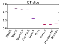
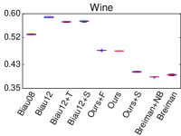
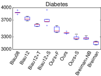
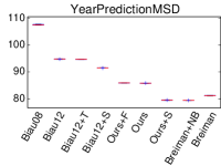
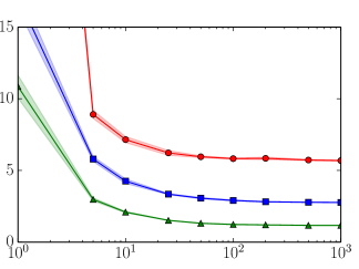
Figure 2 compares the performance of several different random forest algorithm variants on the four UCI data sets. The clear trend here is that Breiman’s algorithm outperforms our own, which in turn outperforms both algorithms from Biau. Generally Biau12 outperforms Biau08, except in the wine quality data set where, strangely, the order is reversed.

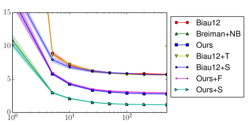
Figure 2 includes a variant of our algorithm which performs data splitting at the forest level, and also a variant of Biau12 which performs data splitting at the tree level. This difference appears to have relatively little effect when there is sufficient data; however, for the Diabetes dataset, which is comparatively small, splitting at the tree instead of the forest level significantly improves performance.

In all cases the gap between Biau12 and our algorithm is larger than the difference in performance from changing how data splitting is done. This indicates that in a practical sense it is the split selection strategy that accounts for most of the improvement of our algorithm over Biau12.

We also experimented with variants of Biau12 and our own algorithm with no data splitting. The most notable thing here is that when data splitting is removed our algorithm is very competitive with Breiman. This indicates that the gap in performance between our algorithm and standard random forests can be contributed almost entirely to data splitting.

We performed all of these experiments using a range of forest sizes. Figure 3 (left) shows performance as a function of forest size. In the interest of space we present this figure only for the CT slice dataset, but the curves for the other datasets tell a similar story. This figure shows that the results from Figure 2 are consistent over a wide range of forest sizes.

Figure 3 (right) more closely examines the effects of the different data splitting and split point selection strategies.

7.2 Kinect Pose Estimation

Figure 4: Left: Depth image with a candidate feature specified by the offsets u and v. Center: Body part labels. Right: Left hand joint predictions (green) made by the appropriate class pixels (blue).

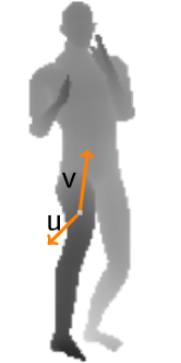
In this section, we evaluate our random forest algorithm on the challenging computer vision problem of predicting the location of human joints from a depth image and corresponding body part labels. See Figure 4 for an example.

Typically the first step in a joint location pipeline is to predict the body part labels of each pixel in the depth image and the second step is to use the labelled pixels to predict joint locations (Shotton et al., 2011).

Since our primary goal is to evaluate regression models rather than to build an end product, we implement only the second step in the basic pipeline. Using depth images with ground truth body part labels for each pixel as training data, we learn a regression model of the offset from a pixel to a joint.

For each joint, we train a forest on the pixels of body parts associated with that joint and predict the relative offset from each pixel to the joint. Typically these errors would be post-processed with mean shift to find a more accurate final prediction for the joint location. We instead report the regression error directly to avoid confounding factors in the comparison between the forest models.

Each joint has its own model that predicts the offset from a pixel to the location of the joint. An offset is predicted for all pixels with body part labels associated with a joint.

Figure 5: Mean squared error in pixel space for a forest of 50 trees on the kinect joint prediction task. Each group of bars shows, from left to right, the error of Biau08, Biau12, Ours and Breiman. The error bars show one standard deviation across 5 runs. Due to space we only include the errors the left side of the body but the results for the right side are similar. In order to make the results legible the $y$-axis is set so that in some cases the error of Biau08 extends vertically off the figure.

To build our data set, we sample random poses from the CMU mocap dataset and render a pair of 320x240 resolution depth and body part images along with the positions of each joint in the skeleton. The 19 body parts and one background class are represented by 20 unique color identifiers in the body part image.

For this experiment we generate 2000 poses for training and 500 poses for testing. To create the training set, we sample 20 pixels without replacement from each body part class in each pose. We then sample 40000 pixels without replacement from the sampled pixels with the associated body part labels across all poses. During testing we evaluate the MSE of the offsets of all pixels associated with a joint. Figure 4 visualizes the raw depth image, ground truth body part labels and the votes for the left hand made by all pixels in the left arm.

The features associated with each pixel are depth differences between pairs of pixels at specified offsets from the target. At training time, candidate pairs of offsets are sampled from a 2-dimensional Gaussian distributions with variance 40.0 (chosen by cross validation). The offsets are scaled by the depth of the target pixel to produce depth invariant features. Figure 4 (left) shows candidate feature offsets $u$ and $v$ for the indicated pixel. The resulting feature value is the depth difference between the pixel at offset $u$ and the pixel at offset $v$. In this experiment we sample 1000 candidate offsets at each node.

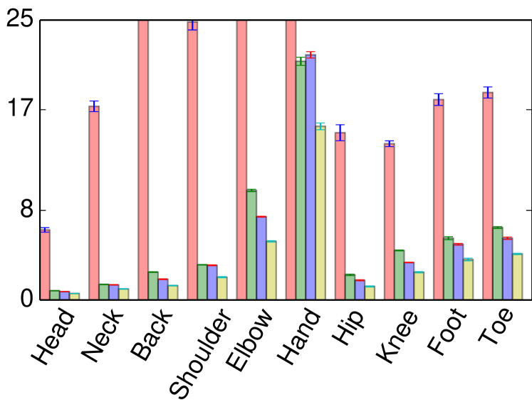
Figure 5 shows the MSE and standard deviation for each joint in pixel units. In the interest of space we only show the joints for the left side of the body but we see similar results for the right side. Just as with the UCI datasets, the dominant ordering from largest to smallest test error is Biau08, Biau12, ours and Breiman.

8 Conclusion

It is fascinating that an algorithm as simple and useful as random forests has turned out to be so difficult to analyze. Motivated by this, we set as our goal to narrow the gap between the theory and practice of regression forests, and we succeeded to a significant extent. Specifically, we were able to derive a new regression forest algorithm, to prove that it is consistent, and to show that its empirical performance is closer to Breiman’s popular model than previous theoretical variants.

Our extensive empirical study, which compares the algorithm widely used in practice to recent theoretical variants for the first time, also casts light on how different design choices and theoretical simplifications impact performance.

We focused on consistency because this is still an important open problem. However, we believe that our theoretical analysis and empirical study help in setting the arena for embarking on other types of analyses, including finite sample size complexity bounds, asymptotic convergence rates, and consistency of random forests in machine learning problems beyond regression.

References

Appendix A Technical results

Lemma 6.

If $U_{1},\ldots U_{m}$ are iid $\operatorname{Uniform}[0,1]$ random variables then

$$\mathbb{E}\left[\max(\max_{i=1}^{m}U_{i},1-\min_{i=1}^{m}U_{i})\right]=\frac{2m+1}{2m+2}$$

Proof.

Let $M_{i}=\max(U_{i},1-U_{i})$, so $M_{i}$ are iid $\operatorname{Uniform}[1/2,1]$ with CDF given by

$$F_{M_{i}}(x)=2x-1$$

for $1/2\leq x\leq 1$. Moreover, if $M=\max_{i=1}^{m}M_{i}$ then $F_{M}(x)=(2x-1)^{m}$ since the $M_{i}$ are iid. The density of $M$ is then

$$f_{M}(x)=\frac{\mathrm{d}}{\mathrm{d}x}F_{M}(x)=2m(2x-1)^{m-1}$$

and its expected value is

$$\mathbb{E}\left[M\right]=\int_{1/2}^{1}xf_{M}(dx)=\frac{2m+1}{2m+2}$$

which proves the claim. ∎

Proposition 7.

For sufficiently large $n$, every cell of the tree will be cut infinitely often in probability. That is, if $K$ is the distance from the root of the tree to a leaf then $P(K<t)\to 0$ for all $t$ as $n\to\infty$.

Proof.

The splitting mechanism functions by choosing $m$ structure points uniformly at random from the node to be split and searching between their min and max. We will refer to the points selected by the splitting mechanism as active. Without loss of generality we can assume the active points are uniformly distributed on $[0,1]$ and lower bound the number of estimation points in the smallest child.

Denote the active points $U_{1},\ldots,U_{m}$ and let $U=\max_{i=1}^{m}(\max(U_{i},1-U_{i}))$. We know from the calculations in Lemma 6 that

$$\mathbb{P}\left(U\leq t\right)=(2t-1)^{m}$$

which means that the length of the smallest child is at least $\delta^{1/K}<1$ with probability $(2(1-\delta^{1/K})-1)^{m}$, i.e.

$$\mathbb{P}\left(U\leq 1-\delta^{1/K}\right)=(2(1-\delta^{1/K})-1)^{m}$$

Repeating this argument $K$ times we have that after $K$ splits all sides of all children have length at least $\delta$ with probability at least $(2(1-\delta^{1/K})-1)^{Km}$. This bound is derived by assuming that the same dimension is cut at each level of the tree. If different dimensions are cut at different levels the probability that all sides have length at least $\delta$ is greater, so the bound holds in those cases also.

This argument shows that every cell at depth $K$ contains a hypercube with sides of length $\delta$ with probability at least $(2(1-\delta^{1/K})-1)^{Km}$. Thus for any $K$ and $\epsilon_{1}>0$ we can pick $\delta$ such that

$$0<\delta^{1/K} \leq 1-\frac{1}{2}((1-\epsilon_{1})^{1/Km}+1)$$

and know that every cell of depth $K$ contains a hypercube with sides of length $\delta$ with probability at least $1-\epsilon_{1}$. Since the distribution of $X$ has a non-zero density, each of these hypercubes has positive measure with respect to $\mu_{X}$. Define

$$p=\min_{L\text{ a leaf at depth }K}\mu_{X}(L)\enspace.$$

We know $p>0$ since the minimum is over finitely many leafs and each leaf contains a set of positive measure.

It remains to show that we can choose $n$ large enough so that any set $A\subset[0,1]^{D}$ with $\mu_{X}(A)\geq p$ contains at least $k_{n}$ estimation points. To this end, fix an arbitrary $A\subset[0,1]^{D}$ with $\mu_{X}(A)=p$. In a data set of size $n$ the number of points which fall in $A$ is $\operatorname{Binomial}(n,p)$. Each point is an estimation point with probability $1/2$, meaning that the number of estimation points, $E_{n}$, in $A$ is $\operatorname{Binomial}(n,p/2)$.

Using Hoeffding’s inequality we can bound $E_{n}$ as follows

$$\mathbb{P}\left(E_{n}<k_{n}\right) \leq\operatorname{exp}\left(-\frac{2}{n}\left(\frac{np}{2}-k_{n}\right)^{2}\right)\leq\operatorname{exp}\left((k_{n}-\frac{np}{2})p\right)\enspace.$$

For this probability to be upper bounded by an arbitrary $\epsilon_{2}>0$ it is sufficient to have

$$\frac{k_{n}}{n} \leq\frac{p}{2}-\frac{1}{np}\log(\frac{1}{\epsilon_{2}})\enspace.$$

The second term goes to zero as $n\to\infty$ so for sufficiently large $n$ the RHS is positive and since $k_{n}/n\to 0$ it is always possible to choose $n$ to satisfy this inequality.

In summary, we have shown that if a branch of the tree is grown to depth $K$ then the leaf at the end of this branch contains a set of positive measure with respect to $\mu_{X}$ with arbitrarily high probability. Moreover, we have shown that if $n$ is sufficiently large this leaf will contain at least $k_{n}$ estimation points.

The only condition which causes our algorithm to terminate leaf expansion is if it is not possible to create child leafs with at least $k_{n}$ points. Since we can make the probability that any leaf at depth $K$ contains at least this many points arbitrarily high, we conclude that by making $n$ large we can make the probability that all branches are actually grown to depth at least $K$ by our algorithm arbitrarily high as well. Since this argument holds for any $K$ the claim is shown. ∎

References

- Amit & Geman (1997) Amit, Y. and Geman, D. Shape quantization and recognition with randomized trees. Neural Computation, 9:1545–1558, 1997.
- Biau (2012) Biau, G. Analysis of a random forests model. Journal of Machine Learning Research, 13:1063–1095, 2012.
- Biau et al. (2008) Biau, G., Devroye, L., and Lugosi, G. Consistency of random forests and other averaging classifiers. Journal of Machine Learning Research, 9:2015–2033, 2008.
- Breiman (1996) Breiman, L. Bagging predictors. Machine Learning, 24(2):123–140, 1996.
- Breiman (2001) Breiman, L. Random forests. Machine Learning, 45(1):5–32, 2001.
- Breiman (2004) Breiman, L. Consistency for a simple model of random forests. Technical report, University of California at Berkeley, 2004.
- Breiman et al. (1984) Breiman, L., Friedman, J., Stone, C., and Olshen, R. Classification and Regression Trees. CRC Press LLC, 1984.
- Criminisi & Shotton (2013) Criminisi, A. and Shotton, J. Decision Forests for Computer Vision and Medical Image Analysis. Springer London, 2013.
- Criminisi et al. (2011) Criminisi, A., Shotton, J, and Konukoglu, E. Decision forests: A unified framework for classification, regression, density estimation, manifold learning and semi-supervised learning. Foundations and Trends in Computer Graphics and Vision, 7(2-3):81–227, 2011.
- Cutler et al. (2007) Cutler, DR., Edwards, T., and Beard, K. Random forests for classification in ecology. Ecology, 88(11):2783–92, 2007.
- Denil et al. (2013) Denil, M., Matheson, D., and de Freitas, N. Consistency of online random forests. In International Conference on Machine Learning, 2013.
- Devroye et al. (1996) Devroye, L., Györfi, L., and Lugosi, G. A Probabilistic Theory of Pattern Recognition. Springer-Verlag, 1996.
- Dietterich (2000) Dietterich, T. G. An experimental comparison of three methods for constructing ensembles of decision trees: Bagging, boosting, and randomization. Machine Learning, pp. 139–157, 2000.
- Genuer (2010) Genuer, R. Risk bounds for purely uniformly random forests. arXiv preprint arXiv:1006.2980, 2010.
- Genuer (2012) Genuer, R. Variance reduction in purely random forests. Journal of Nonparametric Statistics, 24:543–562, 2012.
- Györfi et al. (2002) Györfi, L., Kohler, M., Krzyzak, A., and Walk, H. A Distribution-Free Theory of Nonparametric Regression. Springer, 2002.
- Hastie et al. (2013) Hastie, T., Tibshirani, R., and Friedman, J. The Elements of Statistical Learning. Springer, 10 edition, 2013.
- Ho (1998) Ho, T. K. The random subspace method for constructing decision forests. IEEE Transactions on Pattern Analysis and Machine Intelligence, 20(8):832–844, 1998.
- Ishwaran & Kogalur (2010) Ishwaran, H. and Kogalur, U. B. Consistency of random survival forests. Statistics and probability letters, 80:1056–1064, 2010.
- Kwokt & Carter (1988) Kwokt, S. W. and Carter, C. Multiple decision trees. In Uncertainty in Artificial Intelligence, pp. 213–220, 1988.
- Lin & Jeon (2006) Lin, Y. and Jeon, Y. Random forests and adaptive nearest neighbors. Journal of the American Statistical Association, 101(474):578–590, 2006.
- Meinshausen (2006) Meinshausen, N. Quantile regression forests. Journal of Machine Learning Research, 7:983–999, 2006.
- Montillo et al. (2011) Montillo, A., Shotton, J., Winn, J., Iglesias, J. E., Metaxas, D., and Criminisi, A. Entangled decision forests and their application for semantic segmentation of CT images. In Information Processing in Medical Imaging, pp. 184–196, 2011.
- Prasad et al. (2006) Prasad, A., Iverson, L., and Liaw, A. Newer classification and regression tree techniques: Bagging and random forests for ecological prediction. Ecosystems, 9(2):181–199, 2006.
- Schapire & Freund (2012) Schapire, R. and Freund, Y. Boosting: Foundations and Algorithms. MIT Press, 2012.
- Schroff et al. (2008) Schroff, F., Criminisi, A., and Zisserman, A. Object class segmentation using random forests. In Procedings of the British Machine Vision Conference, pp. 54.1–54.10, 2008.
- Shotton et al. (2011) Shotton, J., Fitzgibbon, A., Cook, M., Sharp, T., Finocchio, M., Moore, R., Kipman, A., and Blake, A. Real-time human pose recognition in parts from single depth images. IEEE Computer Vision and Pattern Recognition, pp. 1297–1304, 2011.
- Svetnik et al. (2003) Svetnik, V., Liaw, A., Tong, C., Culberson, J., Sheridan, R., and Feuston, B. Random forest: a classification and regression tool for compound classification and QSAR modeling. Journal of Chemical Information and Computer Sciences, 43(6):1947–58, 2003.
- Xiong et al. (2012) Xiong, C., Johnson, D., Xu, R., and Corso, J. J. Random forests for metric learning with implicit pairwise position dependence. In ACM SIGKDD International Conference on Knowledge Discovery and Data Mining, pp. 958–966, 2012.
- Zikic et al. (2012) Zikic, D., Glocker, B., and Criminisi, A. Atlas encoding by randomized forests for efficient label propagation. In International Conference on Medical Image Computing and Computer Assisted Intervention, 2012.