Measuring nonlocal Lagrangian peak bias

Matteo Biagetti1, Kwan Chuen Chan1, Vincent Desjacques1 & Aseem Paranjape2
1 Département de Physique Théorique and Center for Astroparticle Physics (CAP), Université de Genève,
24 quai Ernest Ansermet, CH-1211 Genève, Switzerland
2 Instt. for Astronomy, Dept. of Physics, ETH Zürich, Wolfgang-Pauli-Strasse 27, CH-8093 Zürich, Switzerland
E-mail: Vincent.Desjacques@unige.ch
Abstract

We investigate nonlocal Lagrangian bias contributions involving gradients of the linear density field, for which we have predictions from the excursion set peak formalism. We begin by writing down a bias expansion which includes all the bias terms, including the nonlocal ones. Having checked that the model furnishes a reasonable fit to the halo mass function, we develop a 1-point cross-correlation technique to measure bias factors associated with χ2superscript𝜒2\chi^{2}-distributed quantities. We validate the method with numerical realizations of peaks of Gaussian random fields before we apply it to N-body simulations. We focus on the lowest (quadratic) order nonlocal contributions 2χ10(𝐤1𝐤2)2subscript𝜒10subscript𝐤1subscript𝐤2-2\chi_{10}(\mathrm{\bf k}_{1}\cdot\mathrm{\bf k}_{2}) and χ01[3(𝐤1𝐤2)2k12k22]subscript𝜒01delimited-[]3superscriptsubscript𝐤1subscript𝐤22superscriptsubscript𝑘12superscriptsubscript𝑘22\chi_{01}[3(\mathrm{\bf k}_{1}\cdot\mathrm{\bf k}_{2})^{2}-k_{1}^{2}k_{2}^{2}], where 𝐤1subscript𝐤1\mathrm{\bf k}_{1}, 𝐤2subscript𝐤2\mathrm{\bf k}_{2} are wave modes. We can reproduce our measurement of χ10subscript𝜒10\chi_{10} if we allow for an offset between the Lagrangian halo center-of-mass and the peak position. The sign and magnitude of χ10subscript𝜒10\chi_{10} is consistent with Lagrangian haloes sitting near linear density maxima. The resulting contribution to the halo bias can safely be ignored for M=1013M/h𝑀superscript1013subscriptMdirect-productM=10^{13}\ {\rm M_{\odot}/{\it h}}, but could become relevant at larger halo masses. For the second nonlocal bias χ01subscript𝜒01\chi_{01} however, we measure a much larger magnitude than predicted by our model. We speculate that some of this discrepancy might originate from nonlocal Lagrangian contributions induced by nonspherical collapse.

keywords:
cosmology: theory, dark matter, large-scale structure of Universe
pagerange: Measuring nonlocal Lagrangian peak biasB

1 Introduction

Understanding the clustering of dark matter haloes has been a topic of active research for many years. A number of analytic approaches have been developed to tackle this issue such as the peak model (Bardeen et al., 1986), the excursion set framework (Bond et al., 1991) or perturbation theory (see e.g. Bernardeau et al., 2002, for a review). Heuristic arguments like the peak-background split (Kaiser, 1984), and approximations like local bias (Fry & Gaztanaga, 1993) have been very helpful for modelling the clustering of dark matter haloes. Nevertheless, improvements in computational power and numerical algorithms as well as the advent of large scale galaxy surveys have considerably increased the need for an accurate description of halo clustering. Until recently however, it was unclear how the peak approach, which is thus far the only framework in which biased tracers form a discrete point set, relates to the more widespread excursion set theory, local bias approximation or peak-background split argument.

Working out this connection has been the subject of several recent papers. Desjacques (2013), building on earlier work by Desjacques et al. (2010), showed that correlation functions of discrete density peaks can be computed using an effective (i.e. which does not involve measurable counts-in-cells quantities) generalized bias expansion in which all the bias parameters, including those of the nonlocal terms 111To facilitate the comparison with other studies, we will call nonlocal terms all contributions to Lagrangian clustering that are not of the form δn(𝐱)superscript𝛿𝑛𝐱\delta^{n}(\mathrm{\bf x}), where δ(𝐱)𝛿𝐱\delta(\mathrm{\bf x}) is the linear mass density field., can be computed from a peak-background split. In parallel, Paranjape & Sheth (2012) demonstrated how the peak formalism, which deals with statistics of density maxima at a fixed smoothing scale, can be combined with excursion set theory, whose basic building block is the density contrast at various filtering scales. Similar ideas can already be found in the early work of Bond (1989). Paranjape, Sheth & Desjacques (2013) (hereafter PSD) subsequently computed the mass function and linear bias of haloes within this excursion set peak (ESP) approach and showed that it agrees very well with simulation data.

The focus of this work is on the second-order nonlocal bias terms predicted by the ESP approach. These generate corrections to the Fourier peak bias of the form 2χ10(𝐤1𝐤2)2subscript𝜒10subscript𝐤1subscript𝐤2-2\chi_{10}(\mathrm{\bf k}_{1}\cdot\mathrm{\bf k}_{2}) and χ01[3(𝐤1𝐤2)2k12k22]subscript𝜒01delimited-[]3superscriptsubscript𝐤1subscript𝐤22superscriptsubscript𝑘12superscriptsubscript𝑘22\chi_{01}[3(\mathrm{\bf k}_{1}\cdot\mathrm{\bf k}_{2})^{2}-k_{1}^{2}k_{2}^{2}] (Desjacques, 2013). What makes them quite interesting is the fact that there are related to χ2superscript𝜒2\chi^{2} rather than normally-distributed variables. Here, we will show how one can measure their amplitude in the bias of dark matter haloes without computing any correlation function. Of course, this technique can also be applied to measure nonlocal Lagrangian bias contributions induced by e.g. the tidal shear, but this will be the subject of future work.

This paper is organized as follows. In a first part, we will advocate a slight modification of the original excursion set peak formulation of PSD in order to easily write down the corresponding effective bias expansion (Sec. §2). Next, we will explain how the cross-correlation technique proposed by Musso, Paranjape & Sheth (2012), which has already been successfully applied to the bias factors associated with the density field (Paranjape, Sheth & Desjacques, 2013; Paranjape et al., 2013), can be extended to measure the second-order nonlocal bias factors χ10subscript𝜒10\chi_{10} and χ01subscript𝜒01\chi_{01} that weight the two quadratic, nonlocal bias contributions (Sec. §3). Finally, we will validate our method with peaks of Gaussian random fields before measuring χ10subscript𝜒10\chi_{10} and χ01subscript𝜒01\chi_{01} for dark matter haloes (Sec. §4). We conclude in §5.

2 Excursion set peaks

In this section we apply the excursion set approach to the peak model in the case of a moving barrier to get a prediction of the halo mass function which we compare to simulations. We then get expressions for bias parameters, generalising results in Desjacques (2013); Desjacques, Gong & Riotto (2013). We also point out a few changes to PSD. We show that, as far as the mass function is concerned, these modifications do not make much difference (only few percents, in agreement with what PSD found), but they affect first- and second-order bias parameters, as new terms arise.

2.1 Notation

We will adopt the following notation for the variance of the smoothed density field (linearly extrapolated to present-day) and its derivatives,

σjα2=12π20𝑑kP(k)k2(j+1)Wα2(kRα),subscriptsuperscript𝜎2𝑗𝛼12superscript𝜋2superscriptsubscript0differential-d𝑘𝑃𝑘superscript𝑘2𝑗1superscriptsubscript𝑊𝛼2𝑘subscript𝑅𝛼\sigma^{2}_{j\alpha}=\frac{1}{2\pi^{2}}\int_{0}^{\infty}\!\!dk\,P(k)k^{2(j+1)}W_{\alpha}^{2}(kR_{\alpha})\;, (1)

where P(k)𝑃𝑘P(k) is the power spectrum of the mass density field, Wα(kRα)subscript𝑊𝛼𝑘subscript𝑅𝛼W_{\alpha}(kR_{\alpha}) and the subscript α=G𝛼𝐺\alpha=G or T𝑇T will denote Gaussian or tophat filtering, respectively. Moreover, Rαsubscript𝑅𝛼R_{\alpha} is the Lagrangian smoothing scale (which may depend on the choice of kernel). Denoting δTsubscript𝛿𝑇\delta_{T} and δGsubscript𝛿𝐺\delta_{G} the linear density field smoothed with a tophat and Gaussian filter, respectively, we introduce the variables

ν(𝐱)𝜈𝐱\displaystyle\nu(\mathrm{\bf x}) =1σ0TδT(𝐱)absent1subscript𝜎0𝑇subscript𝛿𝑇𝐱\displaystyle=\frac{1}{\sigma_{0T}}\delta_{T}(\mathrm{\bf x}) (2)
u(𝐱)𝑢𝐱\displaystyle u(\mathrm{\bf x}) =1σ2G2δG(𝐱)absent1subscript𝜎2𝐺superscript2subscript𝛿𝐺𝐱\displaystyle=-\frac{1}{\sigma_{2G}}\nabla^{2}\delta_{G}(\mathrm{\bf x})
μ(𝐱)𝜇𝐱\displaystyle\mu(\mathrm{\bf x}) =dδTdRT(𝐱).absent𝑑subscript𝛿𝑇𝑑subscript𝑅𝑇𝐱\displaystyle=-\frac{d\delta_{T}}{dR_{T}}(\mathrm{\bf x})\;.

Note that, while ν𝜈\nu and u𝑢u have unit variance, μ𝜇\mu is not normalized. We will use the notation μ2=Δ02delimited-⟨⟩superscript𝜇2subscriptsuperscriptΔ20\langle\mu^{2}\rangle=\Delta^{2}_{0} in what follows.

Cross-correlations among these three variables are useful and will be denoted as

νudelimited-⟨⟩𝜈𝑢\displaystyle\langle\nu u\rangle =γ1=σ1X2σ0Tσ2Gabsentsubscript𝛾1superscriptsubscript𝜎1𝑋2subscript𝜎0𝑇subscript𝜎2𝐺\displaystyle=\gamma_{1}=\frac{\sigma_{1X}^{2}}{\sigma_{0T}\sigma_{2G}} (3)
νμdelimited-⟨⟩𝜈𝜇\displaystyle\langle\nu\mu\rangle =γνμ=1σ0T0dk2π2P(k)k2WT(kRT)dWT(kRT)dRTabsentsubscript𝛾𝜈𝜇1subscript𝜎0𝑇superscriptsubscript0𝑑𝑘2superscript𝜋2𝑃𝑘superscript𝑘2subscript𝑊𝑇𝑘subscript𝑅𝑇𝑑subscript𝑊𝑇𝑘subscript𝑅𝑇𝑑subscript𝑅𝑇\displaystyle=\gamma_{\nu\mu}=\frac{1}{\sigma_{0T}}\int_{0}^{\infty}\!\!\frac{dk}{2\pi^{2}}\,P(k)k^{2}W_{T}(kR_{T})\frac{dW_{T}(kR_{T})}{dR_{T}} (4)
uμdelimited-⟨⟩𝑢𝜇\displaystyle\langle u\mu\rangle =γuμ=1σ2G0dk2π2P(k)k4WG(kRG)dWT(kRT)dRT.absentsubscript𝛾𝑢𝜇1subscript𝜎2𝐺superscriptsubscript0𝑑𝑘2superscript𝜋2𝑃𝑘superscript𝑘4subscript𝑊𝐺𝑘subscript𝑅𝐺𝑑subscript𝑊𝑇𝑘subscript𝑅𝑇𝑑subscript𝑅𝑇\displaystyle=\gamma_{u\mu}=\frac{1}{\sigma_{2G}}\int_{0}^{\infty}\!\!\frac{dk}{2\pi^{2}}\,P(k)k^{4}W_{G}(kR_{G})\frac{dW_{T}(kR_{T})}{dR_{T}}\;. (5)

The first-order, mixed spectral moment σ1Xsubscript𝜎1𝑋\sigma_{1X} is

σ1X2=12π2𝑑kP(k)k4WT(kRT)WG(kRG),subscriptsuperscript𝜎21𝑋12superscript𝜋2differential-d𝑘𝑃𝑘superscript𝑘4subscript𝑊𝑇𝑘subscript𝑅𝑇subscript𝑊𝐺𝑘subscript𝑅𝐺\sigma^{2}_{1X}=\frac{1}{2\pi^{2}}\int dkP(k)k^{4}W_{T}(kR_{T})W_{G}(kR_{G})\;, (6)

i.e. one filter is tophat and the other Gaussian.

2.2 First-crossing and moving barrier

2.2.1 Summary of previous results

Let us first summarize the basic ideas behind the excursion set peaks approach introduced by Paranjape & Sheth (2012) and further developed in PSD and Desjacques, Gong & Riotto (2013).

The excursion set approach states that a region of mass M𝑀M has virialized when the overdensity δ(R)𝛿𝑅\delta(R), where RM1/3similar-to𝑅superscript𝑀13R\sim M^{1/3} is the filtering scale associated with the perturbation, reaches the spherical collapse threshold δcsubscript𝛿𝑐\delta_{c} provided that, for any R>Rsuperscript𝑅𝑅R^{\prime}>R, the inequality δ(R)<δc𝛿𝑅subscript𝛿𝑐\delta(R)<\delta_{c} holds. This last condition formally implies an infinite set of contraints (one at each smoothing scale). However, as was shown in Musso & Sheth (2012), the requirement δ(R+ΔR)<δc𝛿𝑅Δ𝑅subscript𝛿𝑐\delta(R+\Delta R)<\delta_{c} with ΔR1much-less-thanΔ𝑅1\Delta R\ll 1 furnishes a very good approximation. This follows from the fact that the trajectory described by δ(R)𝛿𝑅\delta(R) as a function of R𝑅R is highly correlated for large radii. As a result, if δ𝛿\delta crosses δcsubscript𝛿𝑐\delta_{c} at R𝑅R, then it is almost certainly below the threshold at any larger radius.

This first-crossing condition can be combined with the peak constraint, so that peaks on a given smoothing scale are counted only if the inequality above is satisfied. In this case, the effective peak bias expansion introduced in Desjacques (2013) is modified through the presence of a new variable μ𝜇\mu (Eq.5) which, as was shown in Desjacques, Gong & Riotto (2013), reflects the dependence of bias to the first-crossing condition.

2.2.2 Modifications to Paranjape, Sheth & Desjacques (2013)

We made a couple of modifications to the approach of PSD, which we will now describe in more details.

Firstly, PSD used the fact that μu𝜇𝑢\mu\equiv u when Gaussian filtering is also applied to the density field, so that the first-crossing condition can be accounted for with the variable u𝑢u only. When δ𝛿\delta is smoothed with a tophat filter however, one should in principle deal explicitly with μ𝜇\mu and, therefore, consider the trivariate normal distribution 𝒩(ν,u,μ)𝒩𝜈𝑢𝜇{\cal N}(\nu,u,\mu). We will proceed this way.

Secondly, Sheth, Mo & Tormen (2001) argued that, owing to the triaxiality of collapse, the critical density for collapse is not constant and equal to δc=1.68subscript𝛿𝑐1.68\delta_{c}=1.68, but rather distributed around a mean value which increases with decreasing halo mass. Analyses of N-body simulations have confirmed this prediction and showed the scatter around the mean barrier is always significant (Dalal et al., 2008; Robertson et al., 2009; Elia, Ludlow & Porciani, 2011). Since the stochasticity induced by triaxial collapse is somewhat cumbersome to implement in analytic models of halo collapse (see e.g. Hahn & Paranjape, 2014, for a tentative implementation with the peak constraint), we will consider a simple approximation calibrated with numerical simulations (note that it differs from the diffusing barrier approach of Maggiore & Riotto, 2010). Namely, the square-root stochastic barrier

B=δc+βσ0,𝐵subscript𝛿𝑐𝛽subscript𝜎0B=\delta_{c}+\beta\sigma_{0}\;, (7)

wherein the stochastic variable β𝛽\beta closely follows a lognormal distribution, furnishes a good description of the critical collapse threshold as a function of halo mass (Robertson et al., 2009). In PSD, this result was interpreted as follows: each halo “sees” a moving barrier B=δc+βσ0𝐵subscript𝛿𝑐𝛽subscript𝜎0B=\delta_{c}+\beta\sigma_{0} with a value of β𝛽\beta drawn from a lognormal distribution. Therefore, the first-crossing condition becomes

B<δ<B+(B+μ)ΔR,𝐵𝛿𝐵superscript𝐵𝜇Δ𝑅B<\delta<B+\left(B^{\prime}+\mu\right)\Delta R\;, (8)

where the prime designates a derivative w.r.t. the filtering scale. Here however, we will assume that each halo “sees” a constant (flat) barrier, whose height varies from halo to halo. Therefore, we will implement the first-crossing condition simply as

B<δ<B+μΔR.𝐵𝛿𝐵𝜇Δ𝑅B<\delta<B+\mu\,\Delta R\;. (9)

Consequently, the variable μ𝜇\mu will satisfy the constraint μ>0𝜇0\mu>0 rather than μ>B𝜇superscript𝐵\mu>-B^{\prime}.

With the aforementioned modifications, the excursion set peak multiplicity function reads

fESP(νc)subscript𝑓ESPsubscript𝜈𝑐\displaystyle f_{\rm ESP}(\nu_{c}) =(VV)1γνμνc0𝑑βp(β)absent𝑉subscript𝑉1subscript𝛾𝜈𝜇subscript𝜈𝑐superscriptsubscript0differential-d𝛽𝑝𝛽\displaystyle=\left(\frac{V}{V_{*}}\right)\frac{1}{\gamma_{\nu\mu}\nu_{c}}\int_{0}^{\infty}d\beta\,p(\beta) (10)
×0dμμ0duf(u,α=1)𝒩(νc+β,u,μ),\displaystyle\quad\times\int_{0}^{\infty}d\mu\,\mu\int_{0}^{\infty}du\,f(u,\alpha=1)\,\mathcal{N}(\nu_{c}+\beta,u,\mu)\;,

where V𝑉V is the Lagrangian volume associated with the TopHat smoothing filter, Vsubscript𝑉V_{*} is the characteristic volume of peaks, p(β)𝑝𝛽p(\beta) is a log-normal distribution, for which we take β=0.5delimited-⟨⟩𝛽0.5\langle\beta\rangle=0.5 and Var(β)=0.25𝛽0.25(\beta)=0.25 as in PSD, and f(u,α)𝑓𝑢𝛼f(u,\alpha) is the slightly modified form (see Desjacques et al., 2010) of the original curvature function of Bardeen et al. (1986) (see Appendix §A). We can now apply Bayes’ theorem and write 𝒩(ν,u,μ)=𝒩(ν,u)𝒩(μ|ν,u)𝒩𝜈𝑢𝜇𝒩𝜈𝑢𝒩conditional𝜇𝜈𝑢\mathcal{N}(\nu,u,\mu)=\mathcal{N}(\nu,u)\mathcal{N}(\mu|\nu,u). The integral over μ𝜇\mu,

0𝑑μμ𝒩(μ|ν,u),superscriptsubscript0differential-d𝜇𝜇𝒩conditional𝜇𝜈𝑢\int_{0}^{\infty}\!\!d\mu\,\mu\,{\cal N}(\mu|\nu,u)\;, (11)

is the same as in Musso & Sheth (2012) and, therefore, is equal to

μ¯[1+erf(μ¯/2Σ)2+Σ2πμ¯eμ¯2/2Σ2],¯𝜇delimited-[]1erf¯𝜇2Σ2Σ2𝜋¯𝜇superscript𝑒superscript¯𝜇22superscriptΣ2\bar{\mu}\left[\frac{1+{\rm erf}(\bar{\mu}/\sqrt{2}\Sigma)}{2}+\frac{\Sigma}{\sqrt{2\pi}\bar{\mu}}e^{-\bar{\mu}^{2}/2\Sigma^{2}}\right]\;, (12)

where

μ¯¯𝜇\displaystyle\bar{\mu} =u(γuμγ1γνμ1γ12)+(ν+β)(γνμγ1γuμ1γ12)absent𝑢subscript𝛾𝑢𝜇subscript𝛾1subscript𝛾𝜈𝜇1superscriptsubscript𝛾12𝜈𝛽subscript𝛾𝜈𝜇subscript𝛾1subscript𝛾𝑢𝜇1superscriptsubscript𝛾12\displaystyle=u\left(\frac{\gamma_{u\mu}-\gamma_{1}\gamma_{\nu\mu}}{1-\gamma_{1}^{2}}\right)+(\nu+\beta)\left(\frac{\gamma_{\nu\mu}-\gamma_{1}\gamma_{u\mu}}{1-\gamma_{1}^{2}}\right) (13)
Σ2superscriptΣ2\displaystyle\Sigma^{2} =Δ02γνμ22γ1γνμγuμ+γuμ21γ12.absentsuperscriptsubscriptΔ02superscriptsubscript𝛾𝜈𝜇22subscript𝛾1subscript𝛾𝜈𝜇subscript𝛾𝑢𝜇superscriptsubscript𝛾𝑢𝜇21superscriptsubscript𝛾12\displaystyle=\Delta_{0}^{2}-\frac{\gamma_{\nu\mu}^{2}-2\gamma_{1}\gamma_{\nu\mu}\gamma_{u\mu}+\gamma_{u\mu}^{2}}{1-\gamma_{1}^{2}}\;. (14)

Substituting this expression into Eq. (10) and performing numerically the integrals over u𝑢u and β𝛽\beta, we obtain an analytic prediction for the halo mass function without any free parameter. Our ESP mass function differs at most by 2 - 3% over the mass range 10111015M/hsuperscript1011superscript1015subscriptMdirect-product10^{11}-10^{15}\ {\rm M_{\odot}/{\it h}} from that obtained with the prescription of PSD. Likewise, the linear and quadratic local bias parameters are barely affected by our modifications.
Refer to caption
Refer to caption
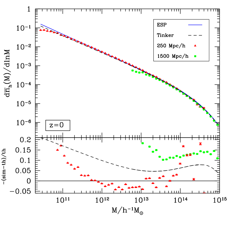
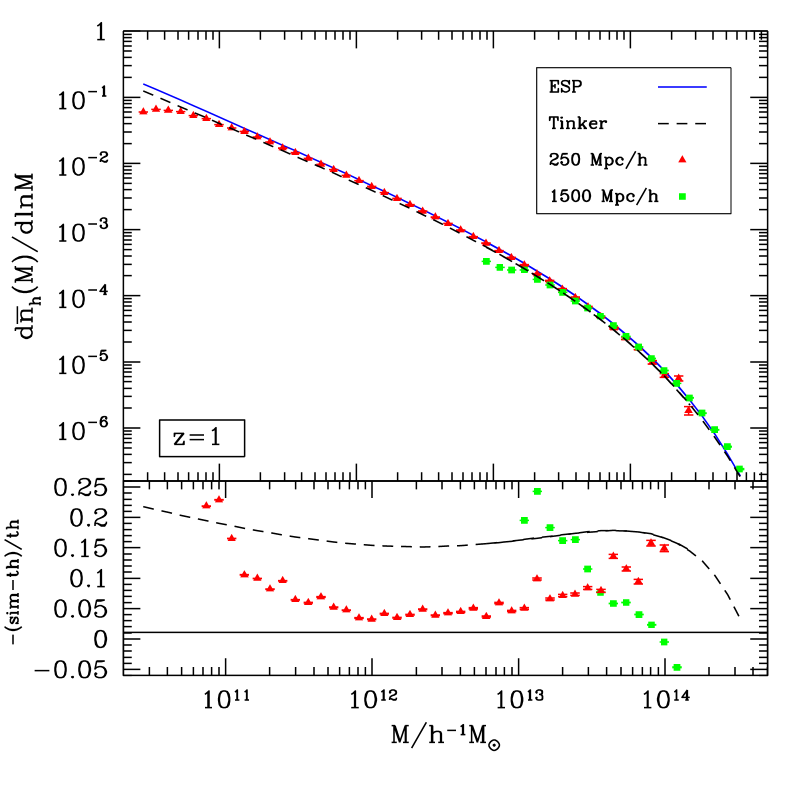
Figure 1: Halo mass function measured from N-body simulation at redshift z=0𝑧0z=0 (left panels) and z=1𝑧1z=1 (right panels) with different box sizes as indicated in the figures. The error bars are Poisson. The data is compared to the theoretical prediction Eq.(15) based on the ESP formalism and the fitting formula of Tinker et al. (2008). We also show the fractional deviation of the Tinker et al. (2008) and the measured halo mass function relative to our theoretical prediction.

2.3 Comparison with numerical simulations

To test the validity of our approach, we compare the ESP mass function with that of haloes extracted from N-body simulations. For this purpose, we ran a series of N-body simulations evolving 10243 particles in periodic cubic boxes of size 1500 and 250h1Mpc250superscript1Mpc250\ {\rm{\it h}^{-1}Mpc}. The particle mass thus is 2.37×10112.37superscript10112.37\times 10^{11} and 1.10×10⁹M/h1.10superscript109subscriptMdirect-product1.10\times 10^{9}\ {\rm M_{\odot}/{\it h}}, respectively. The transfer function was computed with CAMB (Lewis, Challinor & Lasenby, 2000) assuming parameter values consistent with those inferred by WMAP7 (Komatsu et al., 2011): a flat ΛΛ\LambdaCDM cosmology with h=0.7040.704h=0.704, Ωm=0.272subscriptΩm0.272\Omega_{\rm m}=0.272, Ωb=0.0455subscriptΩb0.0455\Omega_{\rm b}=0.0455, ns=0.967subscript𝑛𝑠0.967n_{s}=0.967 and a normalisation amplitude σ8=0.81subscript𝜎80.81\sigma_{8}=0.81. Initial conditions were laid down at redshift z=99𝑧99z=99 with an initial particle displacement computed at 2nd order in Lagrangian perturbation theory with 2LPTic (Crocce, Pueblas & Scoccimarro, 2006). The simulations were run using the N-body code GADGET-2 (Springel, 2005) while the halos were identified with the spherical overdensity (SO) halo finder AHF (Knollmann & Knebe, 2009) assuming an overdensity threshold Δc=200subscriptΔ𝑐200\Delta_{c}=200 constant throughout redshift.

In Fig. (1), we compare the simulated halo mass function to the ESP prediction at redshift z=0𝑧0z=0 and 1. The latter can be straightforwardly obtained from the multiplicity function fESP(νc)subscript𝑓ESPsubscript𝜈𝑐f_{\rm ESP}(\nu_{c}) as

dn¯hdlnM𝑑subscript¯𝑛h𝑑ln𝑀\displaystyle\frac{d\bar{n}_{\rm h}}{d{\rm ln}M} =ρ¯MνcfESP(νc,Rs)dlogνcdlogMabsent¯𝜌𝑀subscript𝜈𝑐subscript𝑓ESPsubscript𝜈𝑐subscript𝑅𝑠𝑑subscript𝜈𝑐𝑑𝑀\displaystyle=\frac{\bar{\rho}}{M}\nu_{c}f_{\rm ESP}(\nu_{c},R_{s})\frac{d\log\nu_{c}}{d\log M} (15)
=3RT(γνμνcσ0T)V1fESP(νc),absent3subscript𝑅𝑇subscript𝛾𝜈𝜇subscript𝜈𝑐subscript𝜎0𝑇superscript𝑉1subscript𝑓ESPsubscript𝜈𝑐\displaystyle=-3R_{T}\left(\frac{\gamma_{\nu\mu}\nu_{c}}{\sigma_{0T}}\right)V^{-1}f_{\rm ESP}(\nu_{c})\;,

where we used the fact that γνμ=σ0Tsubscript𝛾𝜈𝜇superscriptsubscript𝜎0𝑇\gamma_{\nu\mu}=\sigma_{0T}^{\prime} to obtain the second equality. The ESP prediction agrees with the simulations at the 10% level or better from 1014M/hsuperscript1014subscriptMdirect-product10^{14}\ {\rm M_{\odot}/{\it h}} down to a halo mass 1011M/hsuperscript1011subscriptMdirect-product10^{11}\ {\rm M_{\odot}/{\it h}}, where the correspondence between virialized halos and initial density peaks should be rather vague. The abundance of very rare clusters with M>1014M/h𝑀superscript1014subscriptMdirect-productM>10^{14}\ {\rm M_{\odot}/{\it h}} is difficult to predict because of exponential sensitivity to δcsubscript𝛿𝑐\delta_{c}. In this respect, it might be more appropriate to work with a critical linear density δc1.60subscript𝛿𝑐1.60\delta_{c}\approx 1.60 if haloes are defined with a fixed nonlinear threshold Δc=200subscriptΔ𝑐200\Delta_{c}=200 relative to the mean density (see, e.g. Barkana, 2004; Valageas, 2009, for a discussion).

2.4 Bias parameters

The bias factors of ESP peaks can be computed using the same formulae as in Desjacques (2013). With the additional variable μ𝜇\mu, the “localized” number density (in the terminology of Matsubara, 2012) can be written as (Desjacques, Gong & Riotto, 2013)

nESP(𝐰)=(μγνμνc)θH(μ)npk(𝐲),subscript𝑛ESP𝐰𝜇subscript𝛾𝜈𝜇subscript𝜈𝑐subscript𝜃𝐻𝜇subscript𝑛pk𝐲n_{\rm ESP}({\bf w})=-\left(\frac{\mu}{\gamma_{\nu\mu}\nu_{c}}\right)\theta_{H}(\mu)\,n_{\rm pk}(\mathrm{\bf y})\;, (16)

where npksubscript𝑛pkn_{\rm pk} is the localized number density of BBKS peaks, and 𝐰=(ν,ηi,ζij,μ)(𝐲,μ)𝐰𝜈subscript𝜂𝑖subscript𝜁𝑖𝑗𝜇𝐲𝜇{\bf w}=(\nu,\eta_{i},\zeta_{ij},\mu)\equiv({\bf y},\mu) is a 11-dimensional vector containing all the independent variables of the problem. Therefore,

σ0Tiσ2Gjbijksuperscriptsubscript𝜎0𝑇𝑖superscriptsubscript𝜎2𝐺𝑗subscript𝑏𝑖𝑗𝑘\displaystyle\sigma_{0T}^{i}\sigma_{2G}^{j}b_{ijk} =1n¯ESPd11𝐰nESP(𝐰)Hijk(ν,u,μ)P1(𝐰)absent1subscript¯𝑛ESPsuperscript𝑑11𝐰subscript𝑛ESP𝐰subscript𝐻𝑖𝑗𝑘𝜈𝑢𝜇subscript𝑃1𝐰\displaystyle=\frac{1}{\bar{n}_{\rm ESP}}\int\!\!d^{11}\mathrm{\bf w}\,n_{\rm ESP}(\mathrm{\bf w})H_{ijk}(\nu,u,\mu)P_{1}(\mathrm{\bf w})
σ1G2kχk0superscriptsubscript𝜎1𝐺2𝑘subscript𝜒𝑘0\displaystyle\sigma_{1G}^{2k}\chi_{k0} =(1)kn¯ESPd11𝐰nESP(𝐰)Lk(1/2)(3η22)P1(𝐰)absentsuperscript1𝑘subscript¯𝑛ESPsuperscript𝑑11𝐰subscript𝑛ESP𝐰subscriptsuperscript𝐿12𝑘3superscript𝜂22subscript𝑃1𝐰\displaystyle=\frac{(-1)^{k}}{\bar{n}_{\rm ESP}}\int\!\!d^{11}\mathrm{\bf w}\,n_{\rm ESP}(\mathrm{\bf w})L^{(1/2)}_{k}\!\!\left(\frac{3\eta^{2}}{2}\right)P_{1}(\mathrm{\bf w})
σ2G2kχ0ksuperscriptsubscript𝜎2𝐺2𝑘subscript𝜒0𝑘\displaystyle\sigma_{2G}^{2k}\chi_{0k} =(1)kn¯ESPd11𝐰nESP(𝐰)Lk(3/2)(5ζ22)P1(𝐰).absentsuperscript1𝑘subscript¯𝑛ESPsuperscript𝑑11𝐰subscript𝑛ESP𝐰subscriptsuperscript𝐿32𝑘5superscript𝜁22subscript𝑃1𝐰\displaystyle=\frac{(-1)^{k}}{\bar{n}_{\rm ESP}}\int\!\!d^{11}{\bf w}\,n_{\rm ESP}(\mathrm{\bf w})L^{(3/2)}_{k}\!\!\left(\frac{5\zeta^{2}}{2}\right)P_{1}(\mathrm{\bf w})\;. (17)

Here, P1(𝐰)subscript𝑃1𝐰P_{1}(\mathrm{\bf w}) is the 1-point probability density

P1(𝐰)d11𝐰subscript𝑃1𝐰superscript𝑑11𝐰\displaystyle P_{1}(\mathrm{\bf w})d^{11}\mathrm{\bf w} =𝒩(ν,u,μ)dνdudμ×χ32(3η2)d(3η2)absent𝒩𝜈𝑢𝜇𝑑𝜈𝑑𝑢𝑑𝜇subscriptsuperscript𝜒233superscript𝜂2𝑑3superscript𝜂2\displaystyle=\mathcal{N}(\nu,u,\mu)d\nu dud\mu\times\chi^{2}_{3}(3\eta^{2})d(3\eta^{2}) (18)
×χ52(5ζ2)d(5ζ2)×P(angles),absentsubscriptsuperscript𝜒255superscript𝜁2𝑑5superscript𝜁2𝑃angles\displaystyle\qquad\times\chi^{2}_{5}(5\zeta^{2})d(5\zeta^{2})\times P({\rm angles})\;,

where Hijk(ν,u,μ)subscript𝐻𝑖𝑗𝑘𝜈𝑢𝜇H_{ijk}(\nu,u,\mu) are trivariate Hermite polynomials and χk2(x)superscriptsubscript𝜒𝑘2𝑥\chi_{k}^{2}(x) is a χ2superscript𝜒2\chi^{2}-distribution with k𝑘k degrees of freedom (d.o.f.). The probability density P𝑃P(angles) (which was missing 222We thank Marcello Musso for pointing this out to us. in Desjacques, 2013) represents the probability distribution of the 5 remaining degrees of freedom. Since they are all angular variables, they do not generate bias factors because the peak (and halo) overabundance can only depend on scalar quantities (e.g. Catelan, Matarrese & Porciani, 1998; McDonald & Roy, 2009).

The behaviour of the bias factors bij0subscript𝑏𝑖𝑗0b_{ij0} and χklsubscript𝜒𝑘𝑙\chi_{kl} as a function of halo mass is similar to that seen in Fig.1 of Desjacques (2013). The bias factors bijksubscript𝑏𝑖𝑗𝑘b_{ijk} with k1𝑘1k\geq 1 weight the contributions of μksuperscript𝜇𝑘\mu^{k} terms to the clustering of ESP peaks that are proportional to derivatives of the tophat filter w.r.t. the filtering scale RTsubscript𝑅𝑇R_{T}. Similar contributions appear in the clustering of thresholded regions (Matsubara, 2012; Ferraro et al., 2012) since their definition also involve a first-crossing condition.

The effective bias expansion takes the form (Desjacques, 2013; Desjacques, Gong & Riotto, 2013)

δpk(𝐱)subscript𝛿pk𝐱\displaystyle\delta_{\rm pk}(\mathrm{\bf x}) =σ0Tb100ν(𝐱)+σ2Gb010u(𝐱)+b001μ(𝐱)absentsubscript𝜎0𝑇subscript𝑏100𝜈𝐱subscript𝜎2𝐺subscript𝑏010𝑢𝐱subscript𝑏001𝜇𝐱\displaystyle=\sigma_{0T}b_{100}\nu(\mathrm{\bf x})+\sigma_{2G}b_{010}u(\mathrm{\bf x})+b_{001}\mu(\mathrm{\bf x}) (19)
+12σ0T2b200ν2(𝐱)+σ0Tσ2Gb110ν(𝐱)u(𝐱)12superscriptsubscript𝜎0𝑇2subscript𝑏200superscript𝜈2𝐱subscript𝜎0𝑇subscript𝜎2𝐺subscript𝑏110𝜈𝐱𝑢𝐱\displaystyle\quad+\frac{1}{2}\sigma_{0T}^{2}b_{200}\nu^{2}(\mathrm{\bf x})+\sigma_{0T}\sigma_{2G}b_{110}\nu(\mathrm{\bf x})u(\mathrm{\bf x})
+12σ2G2b020u2(𝐱)+12b002μ2(𝐱)12superscriptsubscript𝜎2𝐺2subscript𝑏020superscript𝑢2𝐱12subscript𝑏002superscript𝜇2𝐱\displaystyle\quad+\frac{1}{2}\sigma_{2G}^{2}b_{020}u^{2}(\mathrm{\bf x})+\frac{1}{2}b_{002}\mu^{2}(\mathrm{\bf x})
+σ1G2χ10η2(𝐱)+σ2G2χ01ζ2(𝐱)superscriptsubscript𝜎1𝐺2subscript𝜒10superscript𝜂2𝐱superscriptsubscript𝜎2𝐺2subscript𝜒01superscript𝜁2𝐱\displaystyle\quad+\sigma_{1G}^{2}\chi_{10}\eta^{2}(\mathrm{\bf x})+\sigma_{2G}^{2}\chi_{01}\zeta^{2}(\mathrm{\bf x})
+σ0Tb101ν(𝐱)μ(𝐱)+σ2Gb011u(𝐱)μ(𝐱)+subscript𝜎0𝑇subscript𝑏101𝜈𝐱𝜇𝐱subscript𝜎2𝐺subscript𝑏011𝑢𝐱𝜇𝐱\displaystyle\quad+\sigma_{0T}b_{101}\nu(\mathrm{\bf x})\mu(\mathrm{\bf x})+\sigma_{2G}b_{011}u(\mathrm{\bf x})\mu(\mathrm{\bf x})+\cdots

Here, the rule of thumb is that one should ignore all the terms involving zero-lag moments in the computation of δpk(𝐱1)δpk(𝐱N)delimited-⟨⟩subscript𝛿pksubscript𝐱1subscript𝛿pksubscript𝐱𝑁\langle\delta_{\rm pk}(\mathrm{\bf x}_{1})\dots\delta_{\rm pk}(\mathrm{\bf x}_{N})\rangle in order to correctly predict the N𝑁N-point correlation function, as demonstrated explicitly in Desjacques (2013). The appearance of rotationally invariant quantities is, again, only dictated by the scalar nature of the peak overabundance. The variables of interest here are

η2(𝐱)superscript𝜂2𝐱\displaystyle\eta^{2}(\mathrm{\bf x}) =1σ1G2(δ)2(𝐱)absent1superscriptsubscript𝜎1𝐺2superscript𝛿2𝐱\displaystyle=\frac{1}{\sigma_{1G}^{2}}\left(\nabla\delta\right)^{2}\!(\mathrm{\bf x}) (20)
ζ2(𝐱)superscript𝜁2𝐱\displaystyle\zeta^{2}(\mathrm{\bf x}) =32σ2G2tr[(ijδ13δij2δ)2](𝐱),absent32superscriptsubscript𝜎2𝐺2trdelimited-[]superscriptsubscript𝑖subscript𝑗𝛿13subscript𝛿𝑖𝑗superscript2𝛿2𝐱\displaystyle=\frac{3}{2\sigma_{2G}^{2}}{\rm tr}\!\biggl{[}\Bigl{(}\partial_{i}\partial_{j}\delta-\frac{1}{3}\delta_{ij}\nabla^{2}\delta\Bigr{)}^{2}\biggr{]}\!(\mathrm{\bf x})\;,

so that 3η2(𝐱)3superscript𝜂2𝐱3\eta^{2}(\mathrm{\bf x}) and 5ζ2(𝐱)5superscript𝜁2𝐱5\zeta^{2}(\mathrm{\bf x}) are χ2superscript𝜒2\chi^{2}-distributed with 3 and 5 d.o.f., respectively.

3 Biases from cross-correlation: extension to χ2superscript𝜒2\chi^{2} variables

In this Section, we will demonstrate that the bias factors χijsubscript𝜒𝑖𝑗\chi_{ij} can be measured with a one-point statistics. We will test our method on density peaks of a Gaussian random field before applying it to dark matter halos.

3.1 Bias factors bijksubscript𝑏𝑖𝑗𝑘b_{ijk}: Hermite polynomials

Musso, Paranjape & Sheth (2012) showed that the bias factors of discrete tracers (relative to the mass density δ𝛿\delta) can be computed from one-point measurements rather than computationally more expensive n𝑛n-point correlations. Their idea was implemented by Paranjape, Sheth & Desjacques (2013); Paranjape et al. (2013) to haloes extracted from N-body simulations in order to test the predictions of the ESP formalism. Namely, haloes were traced back to their “proto-halo” patch (since one is interested in measuring Lagrangian biases) in the initial conditions, the linear density field was smoothed on some “large scale” Rlsubscript𝑅𝑙R_{l} and the quantity Hn(νl=δl/σ0l)subscript𝐻𝑛subscript𝜈𝑙subscript𝛿𝑙subscript𝜎0𝑙H_{n}(\nu_{l}=\delta_{l}/\sigma_{0l}) was computed (for n=1,2𝑛12n=1,2 only) at the location of each proto-halo. The average of Hn(νl)subscript𝐻𝑛subscript𝜈𝑙H_{n}(\nu_{l}) over all proto-haloes reads

1Ni=1NHn(νl)=+dνl𝒩(νl)1+δh|νlHn(νl),\frac{1}{N}\sum_{i=1}^{N}H_{n}(\nu_{l})=\int_{-\infty}^{+\infty}\!\!d\nu_{l}\,{\cal N}(\nu_{l})\bigl{\langle}1+\delta_{h}\bigl{\lvert}\nu_{l}\bigr{\rangle}H_{n}(\nu_{l})\;, (21)

where δhsubscript𝛿\delta_{h} is the overdensity of proto-haloes. This expression assumes that the first-crossing condition can be implemented through a constraint of the form Eq.(9), so that P(νl)𝑃subscript𝜈𝑙P(\nu_{l}) is well approximated by a Gaussian (Musso, Paranjape & Sheth, 2012). For the ESP peaks considered here, this ensemble average reads

1n¯ESP+𝑑νl1subscript¯𝑛ESPsuperscriptsubscriptdifferential-dsubscript𝜈𝑙\displaystyle\frac{1}{\bar{n}_{\rm ESP}}\int_{-\infty}^{+\infty}\!\!d\nu_{l} 𝒩(νl)nESP|νlHn(νl)\displaystyle\,{\cal N}(\nu_{l})\bigl{\langle}n_{\rm ESP}\bigl{\lvert}\nu_{l}\bigr{\rangle}H_{n}(\nu_{l}) (22)
=1n¯ESPd11𝐰nESP(𝐰)(ϵν)nabsent1subscript¯𝑛ESPsuperscript𝑑11𝐰subscript𝑛ESP𝐰superscriptsubscriptitalic-ϵ𝜈𝑛\displaystyle=\frac{1}{\bar{n}_{\rm ESP}}\int\!\!d^{11}\mathrm{\bf w}\,n_{\rm ESP}(\mathrm{\bf w})\,\left(-\epsilon_{\nu}\right)^{n}
×(ν+ϵuϵνu+ϵμϵνμ)nP1(𝐰).absentsuperscript𝜈subscriptitalic-ϵ𝑢subscriptitalic-ϵ𝜈𝑢subscriptitalic-ϵ𝜇subscriptitalic-ϵ𝜈𝜇𝑛subscript𝑃1𝐰\displaystyle\qquad\times\left(\frac{\partial}{\partial\nu}+\frac{\epsilon_{u}}{\epsilon_{\nu}}\frac{\partial}{\partial u}+\frac{\epsilon_{\mu}}{\epsilon_{\nu}}\frac{\partial}{\partial\mu}\right)^{n}P_{1}(\mathrm{\bf w})\;.

Here, ϵXsubscriptitalic-ϵ𝑋\epsilon_{X} denotes the cross-correlation between νlsubscript𝜈𝑙\nu_{l} and the variables X=(ν,u,μ)𝑋𝜈𝑢𝜇X=(\nu,u,\mu) defined at the halo smoothing scale. The right-hand side reduces to a sum of n𝑛nth-order bias factors bijksubscript𝑏𝑖𝑗𝑘b_{ijk} weighted by products of ϵνsubscriptitalic-ϵ𝜈\epsilon_{\nu}, ϵusubscriptitalic-ϵ𝑢\epsilon_{u} and ϵμsubscriptitalic-ϵ𝜇\epsilon_{\mu}. Relations between bias factors of a given order (which arise owing to their close connection with Hermite polynomials, see e.g. Musso, Paranjape & Sheth, 2012) can then be used to extract a measurement of each bijksubscript𝑏𝑖𝑗𝑘b_{ijk}.

Refer to caption
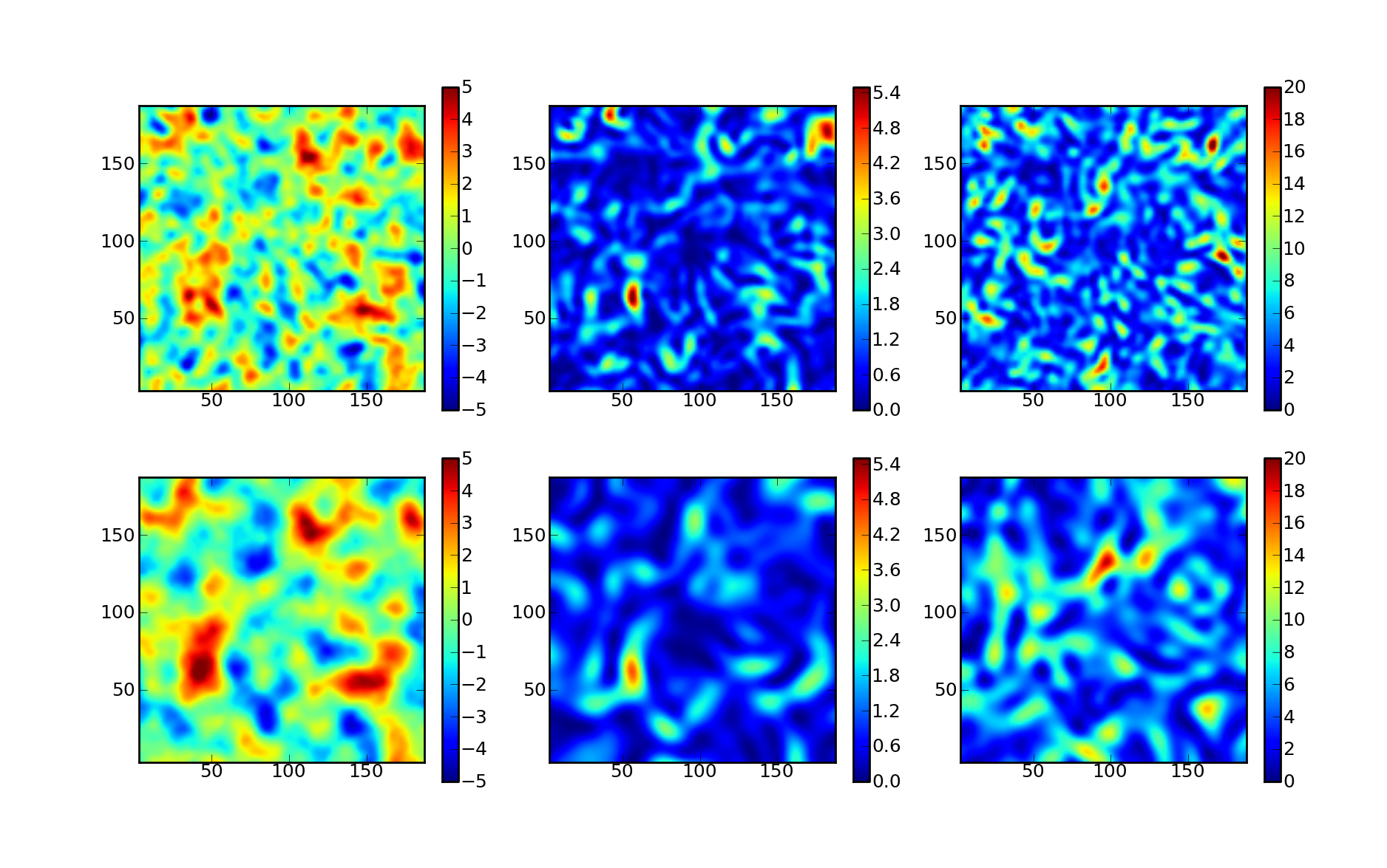
Figure 2: Sections for νlsubscript𝜈𝑙\nu_{l}, 3ηl23superscriptsubscript𝜂𝑙23\eta_{l}^{2} and 5ζl25superscriptsubscript𝜁𝑙25\zeta_{l}^{2} (from left to right). A filtering scale of Rl=5subscript𝑅𝑙5R_{l}=5 and 10h1Mpcsuperscript1Mpc\ {\rm{\it h}^{-1}Mpc} is used for the first and second row, respectively. Note that a tophat kernel is applied for νlsubscript𝜈𝑙\nu_{l}, while a Gaussian window is used for ηl2superscriptsubscript𝜂𝑙2\eta_{l}^{2} and ζl2superscriptsubscript𝜁𝑙2\zeta_{l}^{2}. In each panel, the dimension of the section is 200×\times200 h2superscript2{\it h}^{-2}Mpc2.

Before we generalize this approach to the chi-squared bias factors χijsubscript𝜒𝑖𝑗\chi_{ij}, we emphasize that, in this cross-correlation approach, the smoothing scale Rlsubscript𝑅𝑙R_{l} can take any value as long as it is distinct from the halo smoothing scale. Paranjape et al. (2013) chose RlRsmuch-greater-thansubscript𝑅𝑙subscript𝑅𝑠R_{l}\gg R_{s} in the spirit of the peak-background split but this requirement is, in fact, not necessary as long as the correlation between the two scales is taken into account. In any case, we will stick with the notation Rlsubscript𝑅𝑙R_{l} for convenience.

3.2 Bias factors χijsubscript𝜒𝑖𝑗\chi_{ij}: Laguerre polynomials

The approach presented above can be generalised to χ2superscript𝜒2\chi^{2} distributions. The main difference is the appearance of Laguerre polynomials Ln(α)superscriptsubscript𝐿𝑛𝛼L_{n}^{(\alpha)}. Consider for instance the χ2superscript𝜒2\chi^{2}-quantity 3η23superscript𝜂23\eta^{2} smoothed at the scale Rlsubscript𝑅𝑙R_{l}, i.e. 3ηl23superscriptsubscript𝜂𝑙23\eta_{l}^{2}. In analogy with Eq.(21), the ensemble average of Ln(1/2)(3ηl2)superscriptsubscript𝐿𝑛123superscriptsubscript𝜂𝑙2L_{n}^{(1/2)}(3\eta_{l}^{2}) at the peak positions is

1Ni=1NLn(1/2)(3ηl22)1𝑁superscriptsubscript𝑖1𝑁superscriptsubscript𝐿𝑛123superscriptsubscript𝜂𝑙22\displaystyle\frac{1}{N}\sum_{i=1}^{N}L_{n}^{(1/2)}\!\left(\frac{3\eta_{l}^{2}}{2}\right) =0d(3ηl2)χ32(3ηl2)absentsuperscriptsubscript0𝑑3superscriptsubscript𝜂𝑙2superscriptsubscript𝜒323superscriptsubscript𝜂𝑙2\displaystyle=\int_{0}^{\infty}\!\!d(3\eta_{l}^{2})\,\chi_{3}^{2}(3\eta_{l}^{2}) (23)
×1+δh|3ηl2Ln(1/2)(3ηl22).\displaystyle\qquad\times\bigl{\langle}1+\delta_{h}\bigl{\lvert}3\eta_{l}^{2}\bigr{\rangle}L_{n}^{(1/2)}\!\!\left(\frac{3\eta_{l}^{2}}{2}\right)\;.

The conditional average 1+δh|3ηl2\bigl{\langle}1+\delta_{h}\bigl{\lvert}3\eta_{l}^{2}\bigr{\rangle} reads

1+δh|3ηl2\displaystyle\bigl{\langle}1+\delta_{h}\bigl{\lvert}3\eta_{l}^{2}\bigr{\rangle} =1n¯ESPd11𝐰nESP(𝐰)P1(𝐰|3ηl2)\displaystyle=\frac{1}{\bar{n}_{\rm ESP}}\int\!\!d^{11}\mathrm{\bf w}\,n_{\rm ESP}(\mathrm{\bf w})P_{1}\bigl{(}\mathrm{\bf w}\bigl{\lvert}3\eta_{l}^{2}\bigr{)} (24)
=1n¯ESP𝑑u𝑑ν𝑑μ𝒩(ν,u,μ)absent1subscript¯𝑛ESPdifferential-d𝑢differential-d𝜈differential-d𝜇𝒩𝜈𝑢𝜇\displaystyle=\frac{1}{\bar{n}_{\rm ESP}}\int\!\!dud\nu d\mu\,{\cal N}(\nu,u,\mu)
×d(3η2)χ32(3η2|3ηl2)d(5ζ2)χ52(5ζ2)\displaystyle\qquad\times\int\!\!d(3\eta^{2})\,\chi_{3}^{2}(3\eta^{2}|3\eta_{l}^{2})\int\!\!d(5\zeta^{2})\,\chi_{5}^{2}(5\zeta^{2})
×d(angles)P(angles)nESP(𝐰).\displaystyle\qquad\times\int\!\!d(\text{angles})\,P(\text{angles})\,n_{\rm ESP}(\mathrm{\bf w})\;.

We substitute this relation into Eq.(23) and begin with the integration over the variable 3ηl23superscriptsubscript𝜂𝑙23\eta_{l}^{2}.

We use the following relation (which can be inferred from Eq.(7.414) of Gradshteyn & Ryzhik, 1994)

0𝑑xexxj+αLn(α)(x)=(1)nn!j!Γ(j+α+1)(jn)!.superscriptsubscript0differential-d𝑥superscript𝑒𝑥superscript𝑥𝑗𝛼superscriptsubscript𝐿𝑛𝛼𝑥superscript1𝑛𝑛𝑗Γ𝑗𝛼1𝑗𝑛\int_{0}^{\infty}\!\!dx\,e^{-x}x^{j+\alpha}L_{n}^{(\alpha)}\!(x)=\frac{(-1)^{n}}{n!}\frac{j!\,\Gamma(j+\alpha+1)}{(j-n)!}\;. (25)

With the aid of this result and on expanding the conditional χ2superscript𝜒2\chi^{2}-distribution χ32(3η2|3ηl2)superscriptsubscript𝜒32conditional3superscript𝜂23superscriptsubscript𝜂𝑙2\chi_{3}^{2}(3\eta^{2}|3\eta_{l}^{2}) in Laguerre polynomials (see Appendix §B for details), we obtain

0superscriptsubscript0\displaystyle\int_{0}^{\infty}\!\! d(3ηl2)χ32(3ηl2)Ln(1/2)(3ηl22)χ32(3η2|3ηl2)𝑑3superscriptsubscript𝜂𝑙2superscriptsubscript𝜒323superscriptsubscript𝜂𝑙2superscriptsubscript𝐿𝑛123superscriptsubscript𝜂𝑙22superscriptsubscript𝜒32conditional3superscript𝜂23superscriptsubscript𝜂𝑙2\displaystyle d(3\eta_{l}^{2})\,\chi_{3}^{2}(3\eta_{l}^{2})\,L_{n}^{(1/2)}\!\left(\frac{3\eta_{l}^{2}}{2}\right)\,\chi_{3}^{2}(3\eta^{2}|3\eta_{l}^{2}) (26)
=(1)nn!1Γ(3/2)(3η22)αe3η2/2(1ϵ2)2(1ϵ2)α+1absentsuperscript1𝑛𝑛1Γ32superscript3superscript𝜂22𝛼superscript𝑒3superscript𝜂221superscriptitalic-ϵ22superscript1superscriptitalic-ϵ2𝛼1\displaystyle=\frac{(-1)^{n}}{n!}\frac{1}{\Gamma(3/2)}\left(\frac{3\eta^{2}}{2}\right)^{\alpha}\frac{e^{-3\eta^{2}/2(1-\epsilon^{2})}}{2\left(1-\epsilon^{2}\right)^{\alpha+1}}
×j=0j!(jn)!(ϵ21ϵ2)jLj(1/2)[3η22(1ϵ2)].\displaystyle\qquad\times\sum_{j=0}^{\infty}\frac{j!}{(j-n)!}\left(\frac{-\epsilon^{2}}{1-\epsilon^{2}}\right)^{j}L_{j}^{(1/2)}\!\left[\frac{3\eta^{2}}{2(1-\epsilon^{2})}\right]\;.

For simplicity, let us consider the case n=0,1𝑛01n=0,1 solely. For n=0𝑛0n=0, the sum simplifies to

j=0(ϵ21ϵ2)jLj(1/2)[3η22(1ϵ2)]=(1ϵ2)3/2exp[(ϵ21ϵ2)3η22],superscriptsubscript𝑗0superscriptsuperscriptitalic-ϵ21superscriptitalic-ϵ2𝑗superscriptsubscript𝐿𝑗12delimited-[]3superscript𝜂221superscriptitalic-ϵ2superscript1superscriptitalic-ϵ232superscriptitalic-ϵ21superscriptitalic-ϵ23superscript𝜂22\sum_{j=0}^{\infty}\left(\frac{-\epsilon^{2}}{1-\epsilon^{2}}\right)^{j}L_{j}^{(1/2)}\!\left[\frac{3\eta^{2}}{2(1-\epsilon^{2})}\right]\\ =\left(1-\epsilon^{2}\right)^{3/2}\exp\!\left[\left(\frac{\epsilon^{2}}{1-\epsilon^{2}}\right)\frac{3\eta^{2}}{2}\right]\;, (27)

and the integral Eq.(26) (L0(1/2)(3ηl2/2)1superscriptsubscript𝐿0123superscriptsubscript𝜂𝑙221L_{0}^{(1/2)}(3\eta_{l}^{2}/2)\equiv 1) is trivially equal to χ32(3η2)superscriptsubscript𝜒323superscript𝜂2\chi_{3}^{2}(3\eta^{2}) (as it should be, since we are essentially marginalizing over 3ηl23superscriptsubscript𝜂𝑙23\eta_{l}^{2}).

For n1𝑛1n\geq 1, the sum can be evaluated upon taking suitable derivatives of the right-hand side of Eq.(27), which indeed is a generating function for the Laguerre polynomials Ln(1/2)superscriptsubscript𝐿𝑛12L_{n}^{(1/2)}. For n=1𝑛1n=1, a little algebra leads to

j=0j(ϵ21ϵ2)j1Lj(1/2)[3η22(1ϵ2)]=(1ϵ2)5/2L1(1/2)(3η22)exp[(ϵ21ϵ2)3η22].superscriptsubscript𝑗0𝑗superscriptsuperscriptitalic-ϵ21superscriptitalic-ϵ2𝑗1superscriptsubscript𝐿𝑗12delimited-[]3superscript𝜂221superscriptitalic-ϵ2superscript1superscriptitalic-ϵ252superscriptsubscript𝐿1123superscript𝜂22superscriptitalic-ϵ21superscriptitalic-ϵ23superscript𝜂22\sum_{j=0}^{\infty}j\left(\frac{-\epsilon^{2}}{1-\epsilon^{2}}\right)^{j-1}L_{j}^{(1/2)}\!\left[\frac{3\eta^{2}}{2(1-\epsilon^{2})}\right]\\ =\left(1-\epsilon^{2}\right)^{5/2}L_{1}^{(1/2)}\!\left(\frac{3\eta^{2}}{2}\right)\exp\left[\left(\frac{\epsilon^{2}}{1-\epsilon^{2}}\right)\frac{3\eta^{2}}{2}\right]\;. (28)

Hence, Eq. (26) with n=1𝑛1n=1 equals ϵ2L1(1/2)(3η2/2)χ32(3η2)superscriptitalic-ϵ2superscriptsubscript𝐿1123superscript𝜂22superscriptsubscript𝜒323superscript𝜂2\epsilon^{2}L_{1}^{(1/2)}(3\eta^{2}/2)\chi_{3}^{2}(3\eta^{2}). Performing the remaining integrals over ν𝜈\nu, u𝑢u, μ𝜇\mu and 5ζ25superscript𝜁25\zeta^{2} (the integral over the angles is trivially unity) and taking into account the ESP peak constraint through the multiplicative factor nESP(𝐰)subscript𝑛ESP𝐰n_{\rm ESP}(\mathrm{\bf w}), Eq.(23) simplifies to

0d(3ηl2)χ32(3ηl2)1+δh|3ηl2L1(1/2)(3ηl22)=ϵ2σ12χ10\int_{0}^{\infty}\!\!d(3\eta_{l}^{2})\,\chi_{3}^{2}(3\eta_{l}^{2})\,\bigl{\langle}1+\delta_{h}\bigl{\lvert}3\eta_{l}^{2}\bigr{\rangle}\,L_{1}^{(1/2)}\!\!\left(\frac{3\eta_{l}^{2}}{2}\right)=-\epsilon^{2}\sigma_{1}^{2}\chi_{10} (29)

For the variable 3η23superscript𝜂23\eta^{2}, the cross-correlation coefficient ϵitalic-ϵ\epsilon is

ϵ2η2ηl2η2ηl2(η4η22)(ηl4ηl22)=(σ1×2σ1sσ1l)2,superscriptitalic-ϵ2delimited-⟨⟩superscript𝜂2superscriptsubscript𝜂𝑙2delimited-⟨⟩superscript𝜂2delimited-⟨⟩superscriptsubscript𝜂𝑙2delimited-⟨⟩superscript𝜂4superscriptdelimited-⟨⟩superscript𝜂22delimited-⟨⟩superscriptsubscript𝜂𝑙4superscriptdelimited-⟨⟩superscriptsubscript𝜂𝑙22superscriptsuperscriptsubscript𝜎12subscript𝜎1𝑠subscript𝜎1𝑙2\epsilon^{2}\equiv\frac{\bigl{\langle}\eta^{2}\eta_{l}^{2}\bigr{\rangle}-\bigl{\langle}\eta^{2}\bigr{\rangle}\bigl{\langle}\eta_{l}^{2}\bigr{\rangle}}{\sqrt{\left(\bigl{\langle}\eta^{4}\bigr{\rangle}-\bigl{\langle}\eta^{2}\bigr{\rangle}^{2}\right)\left(\bigl{\langle}\eta_{l}^{4}\bigr{\rangle}-\bigl{\langle}\eta_{l}^{2}\bigr{\rangle}^{2}\right)}}=\left(\frac{\sigma_{1\times}^{2}}{\sigma_{1s}\sigma_{1l}}\right)^{2}\;, (30)

which we shall denote as ϵ1subscriptitalic-ϵ1\epsilon_{1} in what follows. Furthermore,

σn×2=12π20𝑑kk2(n+1)P(k)WG(kRs)WG(kRl)superscriptsubscript𝜎𝑛212superscript𝜋2superscriptsubscript0differential-d𝑘superscript𝑘2𝑛1𝑃𝑘subscript𝑊𝐺𝑘subscript𝑅𝑠subscript𝑊𝐺𝑘subscript𝑅𝑙\displaystyle\sigma_{n\times}^{2}=\frac{1}{2\pi^{2}}\int_{0}^{\infty}\!\!dk\,k^{2(n+1)}\,P(k)W_{G}(kR_{s})W_{G}(kR_{l}) (31)

designates the splitting of filtering scales, i.e. one filter is on scale Rssubscript𝑅𝑠R_{s} while the second is on scale Rlsubscript𝑅𝑙R_{l}. It should be noted that, unlike σ1Xsubscript𝜎1X\sigma_{1{\rm\small X}} defined in Eq.(6), both filtering kernels are Gaussian.

The derivation of the bias factors χ0ksubscript𝜒0𝑘\chi_{0k} associated with the quadratic variable ζ2superscript𝜁2\zeta^{2} proceeds analogously. In particular,

0d(5ζl2)χ52(5ζl2)1+δh|5ζl2L1(3/2)(5ζl22)=ϵ2σ22χ01.\int_{0}^{\infty}\!\!d(5\zeta_{l}^{2})\,\chi_{5}^{2}(5\zeta_{l}^{2})\,\bigl{\langle}1+\delta_{h}\bigl{\lvert}5\zeta_{l}^{2}\bigr{\rangle}\,L_{1}^{(3/2)}\!\!\left(\frac{5\zeta_{l}^{2}}{2}\right)=-\epsilon^{2}\sigma_{2}^{2}\chi_{01}\;. (32)

Here, the cross-correlation coefficient is ϵ=σ2×2/(σ2sσ2l)ϵ2italic-ϵsuperscriptsubscript𝜎22subscript𝜎2𝑠subscript𝜎2𝑙subscriptitalic-ϵ2\epsilon=\sigma_{2\times}^{2}/(\sigma_{2s}\sigma_{2l})\equiv\epsilon_{2}. Note that, in both cases, the cross-correlation coefficient drops very rapidly as Rlsubscript𝑅𝑙R_{l} moves away from Rssubscript𝑅𝑠R_{s} for realistic CDM power spectra. In addition, one could in principle choose Rl<Rssubscript𝑅𝑙subscript𝑅𝑠R_{l}<R_{s} (if there is enough numerical resolution) to measure χijsubscript𝜒𝑖𝑗\chi_{ij}.

4 Test with numerical simulations

In this Section, we first validate our predictions based on peaks of Gaussian random fields with measurements extracted from random realizations of the Gaussian linear density field, and then move on to calculate χ10subscript𝜒10\chi_{10} and χ01subscript𝜒01\chi_{01} for M>M𝑀>subscript𝑀M~{}\hbox to0.0pt{$>$\hss}{\lower 4.30554pt\hbox{$\sim$}}M_{\star} haloes, where Msubscript𝑀M_{\star} is the characteristic mass of the haloes.

4.1 Peaks of Gaussian random fields
Refer to caption
Refer to caption
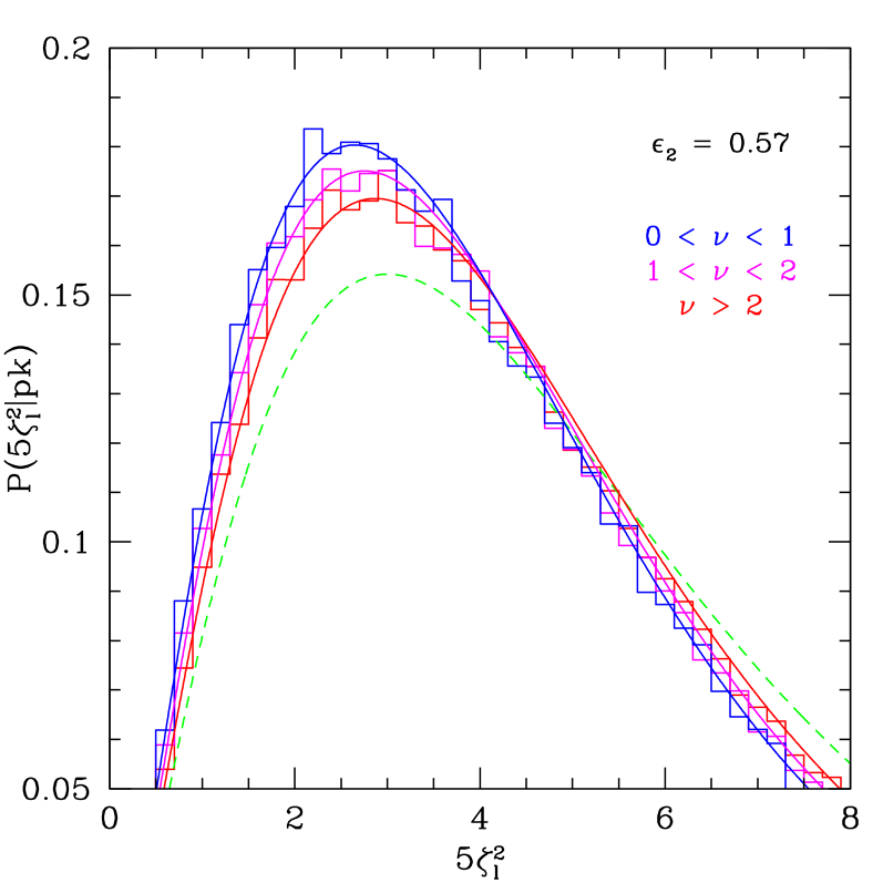
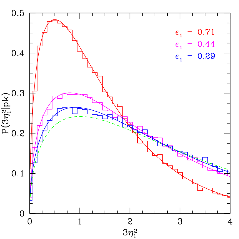
Figure 3: Conditional probability distribution for the variables 3ηl23superscriptsubscript𝜂𝑙23\eta_{l}^{2} (left panel) and 5ζl25superscriptsubscript𝜁𝑙25\zeta_{l}^{2} (right panel) measured at the position of maxima of the linear density field smoothed with a Gaussian filter on scale R=5h1Mpc𝑅5superscript1MpcR=5\ {\rm{\it h}^{-1}Mpc}. Left panel: histrograms indicate the results for Rl=10subscript𝑅𝑙10R_{l}=10, 15 and 20h1Mpc20superscript1Mpc20\ {\rm{\it h}^{-1}Mpc}, which leads to ϵ1=0.71subscriptitalic-ϵ10.71\epsilon_{1}=0.71, 0.44 and 0.29 as quoted on the figure. Right panel: histograms show the results for a fixed Rl=10h1Mpcsubscript𝑅𝑙10superscript1MpcR_{l}=10\ {\rm{\it h}^{-1}Mpc} (which implies ϵ2=0.57subscriptitalic-ϵ20.57\epsilon_{2}=0.57) but several peak height intervals. In all cases, the solid curves are the theoretical prediction (see text) whereas the dashed (green) curves represents the unconditional distribution χk2(y)superscriptsubscript𝜒𝑘2𝑦\chi_{k}^{2}(y).

We generate random realizations of the Gaussian, linear density field with a power spectrum equal to that used to seed the N-body simulations described above. To take advantage of FFTs, we simulate the linear density field in periodic, cubic boxes of side 1000h1Mpcsuperscript1Mpc\ {\rm{\it h}^{-1}Mpc}. The size of the mesh along each dimension is 1536. We smooth the density field on scale Rs=5h1Mpcsubscript𝑅𝑠5superscript1MpcR_{s}=5\ {\rm{\it h}^{-1}Mpc} with a tophat filter and find the local maxima by comparing the density at each grid point with its 26 neighbouring values.

We then smooth the density field on the larger scales Rl=10subscript𝑅𝑙10R_{l}=10, 15 and 20h1Mpcsuperscript1Mpc\ {\rm{\it h}^{-1}Mpc} with a Gaussian filter and compute

ηl2superscriptsubscript𝜂𝑙2\displaystyle\eta_{l}^{2} =1σ1l2(δl)2absent1superscriptsubscript𝜎1𝑙2superscriptsubscript𝛿𝑙2\displaystyle=\frac{1}{\sigma_{1l}^{2}}(\nabla\delta_{l})^{2} (33)
ζl2superscriptsubscript𝜁𝑙2\displaystyle\zeta_{l}^{2} =32σ2l2tr[(ijδl13δij2δl)2].absent32superscriptsubscript𝜎2𝑙2trdelimited-[]superscriptsubscript𝑖subscript𝑗subscript𝛿𝑙13subscript𝛿𝑖𝑗superscript2subscript𝛿𝑙2\displaystyle=\frac{3}{2\sigma_{2l}^{2}}{\rm tr}\!\biggl{[}\Bigl{(}\partial_{i}\partial_{j}\delta_{l}-\frac{1}{3}\delta_{ij}\nabla^{2}\delta_{l}\Bigr{)}^{2}\biggr{]}\;. (34)

These density fields with derivatives sensitively depend on the smoothing scales used. To illustrate this we show in Fig. 2 sections of νlsubscript𝜈𝑙\nu_{l}, 3ηl23superscriptsubscript𝜂𝑙23\eta_{l}^{2} and 5ζl25superscriptsubscript𝜁𝑙25\zeta_{l}^{2}. The sections, each of which of dimensions 200×\times200 h2Mpc2superscript2superscriptMpc2{\rm{\it h}^{-2}Mpc^{2}}, were generated at z=99𝑧99z=99 with the same random seed. The first row corresponds to Rs=5h1Mpcsubscript𝑅𝑠5superscript1MpcR_{s}=5\ {\rm{\it h}^{-1}Mpc}, whereas the second row displays results on the filtering scale Rl=10h1Mpcsubscript𝑅𝑙10superscript1MpcR_{l}=10\ {\rm{\it h}^{-1}Mpc}. We note that, for the normalized density field νlsubscript𝜈𝑙\nu_{l}, an increase in the smoothing scale washes out the small scale features, but the large scale pattern remains. For the quadratic variable ηl2superscriptsubscript𝜂𝑙2\eta_{l}^{2} however, the resemblance between the features at the small and large filtering scale is tenuous. This is even worse for ζl2superscriptsubscript𝜁𝑙2\zeta_{l}^{2}.

Compared to νlsubscript𝜈𝑙\nu_{l}, the fields ηl2superscriptsubscript𝜂𝑙2\eta_{l}^{2} and ζl2superscriptsubscript𝜁𝑙2\zeta_{l}^{2} have one and two additional derivatives which give rise to an effective window function whose isotropic part is given by

Weff(k,R)=kne(kR)2/2,subscript𝑊eff𝑘𝑅superscript𝑘𝑛superscript𝑒superscript𝑘𝑅22W_{\rm eff}(k,R)=k^{n}e^{-(kR)^{2}/2}, (35)

where n=0𝑛0n=0, 1 and 2 are for νlsubscript𝜈𝑙\nu_{l}, ηl2superscriptsubscript𝜂𝑙2\eta_{l}^{2} and ζl2superscriptsubscript𝜁𝑙2\zeta_{l}^{2}, respectively. For n=0𝑛0n=0, the window becomes narrower as Rlsubscript𝑅𝑙R_{l} increases, yet remains unity for wavenumbers k1/Rlless-than-or-similar-to𝑘1subscript𝑅𝑙k\lesssim 1/R_{l}. Weffsubscript𝑊effW_{\rm eff} reaches a maximum at n/R𝑛𝑅\sqrt{n}/R. Hence, for n=1𝑛1n=1 and 2, Weffsubscript𝑊effW_{\rm eff} selects predominantly wavemodes with k1/Rsimilar-to𝑘1𝑅k\sim 1/R. Consequently, since in a Gaussian random field the wavemodes at different scales are uncorrelated, patterns in the fields ηl2superscriptsubscript𝜂𝑙2\eta_{l}^{2} and ζl2superscriptsubscript𝜁𝑙2\zeta_{l}^{2} can change drastically as Rlsubscript𝑅𝑙R_{l} varies. This effect expected to be most significant for n=2𝑛2n=2, i.e. ζl2superscriptsubscript𝜁𝑙2\zeta_{l}^{2}.

For each local density maxima, we store the peak height ν𝜈\nu as well as the value of ηl2superscriptsubscript𝜂𝑙2\eta_{l}^{2} and ζl2superscriptsubscript𝜁𝑙2\zeta_{l}^{2} at the peak position. The left panel of Fig.3 displays as histograms the resulting probability distribution P(3ηl2|pk)𝑃conditional3superscriptsubscript𝜂𝑙2pkP(3\eta_{l}^{2}|{\rm pk}) for three different values of Rl=10subscript𝑅𝑙10R_{l}=10, 15 and 20h1Mpcsuperscript1Mpc\ {\rm{\it h}^{-1}Mpc}. The solid curves represent the theoretical prediction Eq.(48) with x=3η2|pk=0𝑥inner-product3superscript𝜂2pk0x=\langle 3\eta^{2}|{\rm pk}\rangle=0 and ϵ1=0.71subscriptitalic-ϵ10.71\epsilon_{1}=0.71, 0.44 and 0.29 (from the smallest to largest Rlsubscript𝑅𝑙R_{l}) as was measured from the random realizations. The dashed curve is the unconditional χ2superscript𝜒2\chi^{2}-distribution with 3 degrees of freedom. The theory gives excellent agreement with the simulations. Note also that we did not find any evidence for a dependence on the peak height, as expected from the absence of a correlation between ν𝜈\nu and ηl2superscriptsubscript𝜂𝑙2\eta_{l}^{2}. The right panel of Fig.3 shows results for ζl2superscriptsubscript𝜁𝑙2\zeta_{l}^{2}. Here however, since the cross-correlation coefficient diminishes very quickly when Rlsubscript𝑅𝑙R_{l} even slightly departs from Rssubscript𝑅𝑠R_{s}, we show result for Rl=10h1Mpcsubscript𝑅𝑙10superscript1MpcR_{l}=10\ {\rm{\it h}^{-1}Mpc} only, which corresponds to ϵ2=0.57subscriptitalic-ϵ20.57\epsilon_{2}=0.57. In addition, because one should expect a dependence of the shape of the density profile around peaks to the peak height, we consider three different ranges of ν𝜈\nu as indicated on the figure. The solid curves indicate the theoretical prediction Eq.(48) with ϵ2=0.57subscriptitalic-ϵ20.57\epsilon_{2}=0.57 and x=5ζ2|pk𝑥inner-product5superscript𝜁2pkx=\langle 5\zeta^{2}|{\rm pk}\rangle, where

5ζ2|pk=2αlnνminνmax𝑑νG0(α)(γ1,γ1ν).inner-product5superscript𝜁2pk2subscript𝛼lnsuperscriptsubscriptsubscript𝜈minsubscript𝜈maxdifferential-d𝜈superscriptsubscript𝐺0𝛼subscript𝛾1subscript𝛾1𝜈\langle 5\zeta^{2}|{\rm pk}\rangle=-2\partial_{\alpha}{\rm ln}\int_{\nu_{\rm min}}^{\nu_{\rm max}}d\nu\,G_{0}^{(\alpha)}\!(\gamma_{1},\gamma_{1}\nu)\;. (36)

Here, G0(α)superscriptsubscript𝐺0𝛼G_{0}^{(\alpha)} is the integral of f(u,α)𝑓𝑢𝛼f(u,\alpha) over all the allowed peak curvatures. The average 5ζ2|pkinner-product5superscript𝜁2pk\langle 5\zeta^{2}|{\rm pk}\rangle increases with the peak height to reach 5 in the limit ν𝜈\nu\to\infty. The figure shows a clear deviation from the unconditional distribution χ52(5ζl2)superscriptsubscript𝜒525superscriptsubscript𝜁𝑙2\chi_{5}^{2}(5\zeta_{l}^{2}) (shown as the dashed curve) and a dependence on ν𝜈\nu consistent with theoretical predictions.

4.2 Dark matter haloes

Having successfully tested the theory against numerical simulations of Gaussian peaks, we will now attempt to estimate the bias factors χ10subscript𝜒10\chi_{10} and χ01subscript𝜒01\chi_{01} associated with dark matter haloes. For this purpose, we first trace back all dark matter particles belonging to virialized haloes at redshift z=0𝑧0z=0 to their initial position at z=99𝑧99z=99. We then compute the center-of-mass positions of these Lagrangian regions and assume that they define the locations of proto-haloes. We can now proceed as for the Gaussian peaks and compute ν𝜈\nu, ηl2superscriptsubscript𝜂𝑙2\eta_{l}^{2} and ζl2superscriptsubscript𝜁𝑙2\zeta_{l}^{2} at the position of proto-haloes.

The quadratic bias factors χ10subscript𝜒10\chi_{10} and χ01subscript𝜒01\chi_{01} could be in principle computed analogously to Paranjape et al. (2013), i.e. by stacking measurements of ηl2superscriptsubscript𝜂𝑙2\eta_{l}^{2} and ζl2superscriptsubscript𝜁𝑙2\zeta_{l}^{2} at the locations of proto-haloes :

σ1s2χ^10=1Nϵ12i=1NL1(1/2)(3ηl22)superscriptsubscript𝜎1𝑠2subscript^𝜒101𝑁superscriptsubscriptitalic-ϵ12superscriptsubscript𝑖1𝑁superscriptsubscript𝐿1123superscriptsubscript𝜂𝑙22\sigma_{1s}^{2}\hat{\chi}_{10}=-\frac{1}{N\epsilon_{1}^{2}}\sum_{i=1}^{N}L_{1}^{(1/2)}\!\left(\frac{3\eta_{l}^{2}}{2}\right) (37)

and

σ2s2χ^01=1Nϵ22i=1NL1(3/2)(5ζl22).superscriptsubscript𝜎2𝑠2subscript^𝜒011𝑁superscriptsubscriptitalic-ϵ22superscriptsubscript𝑖1𝑁superscriptsubscript𝐿1325superscriptsubscript𝜁𝑙22\sigma_{2s}^{2}\hat{\chi}_{01}=-\frac{1}{N\epsilon_{2}^{2}}\sum_{i=1}^{N}L_{1}^{(3/2)}\!\left(\frac{5\zeta_{l}^{2}}{2}\right)\;. (38)

Here, N𝑁N is the number of halos, s𝑠s designates smoothing at the halo mass scale with a Gaussian filter WGsubscript𝑊𝐺W_{G} on scale RG(RT)subscript𝑅𝐺subscript𝑅𝑇R_{G}(R_{T}), whereas l𝑙l designates Gaussian smoothing at the large scale Rlsubscript𝑅𝑙R_{l}. However, because the cross-correlation coefficient is fairly small unless Rlsubscript𝑅𝑙R_{l} is very close to RGsubscript𝑅𝐺R_{G}, we decided to compute χ10subscript𝜒10\chi_{10} and χ01subscript𝜒01\chi_{01} by fitting the probability distribution P(3ηl2|halo)𝑃conditional3superscriptsubscript𝜂𝑙2haloP(3\eta_{l}^{2}|{\rm halo}) and P(5ζl2|halo)𝑃conditional5superscriptsubscript𝜁𝑙2haloP(5\zeta_{l}^{2}|{\rm halo}) with the conditional χ2superscript𝜒2\chi^{2}-distribution χk2(y|x)superscriptsubscript𝜒𝑘2conditional𝑦𝑥\chi_{k}^{2}(y|x). Namely,

σ1s2χ^10superscriptsubscript𝜎1𝑠2subscript^𝜒10\displaystyle\sigma_{1s}^{2}\hat{\chi}_{10} =12(3η2|halo3)absent12inner-product3superscript𝜂2halo3\displaystyle=\frac{1}{2}\left(\langle 3\eta^{2}|{\rm halo}\rangle-3\right) (39)
σ2s2χ^01superscriptsubscript𝜎2𝑠2subscript^𝜒01\displaystyle\sigma_{2s}^{2}\hat{\chi}_{01} =12(5ζ2|halo5),absent12inner-product5superscript𝜁2halo5\displaystyle=\frac{1}{2}\left(\langle 5\zeta^{2}|{\rm halo}\rangle-5\right)\;,

where 3η2|haloinner-product3superscript𝜂2halo\langle 3\eta^{2}|{\rm halo}\rangle and 5ζ2|haloinner-product5superscript𝜁2halo\langle 5\zeta^{2}|{\rm halo}\rangle are the best-fitting values obtained for x𝑥x. We used measurements obtained at the smoothing scale Rl=10h1Mpcsubscript𝑅𝑙10superscript1MpcR_{l}=10\ {\rm{\it h}^{-1}Mpc} only to maximize the signal.

Refer to caption
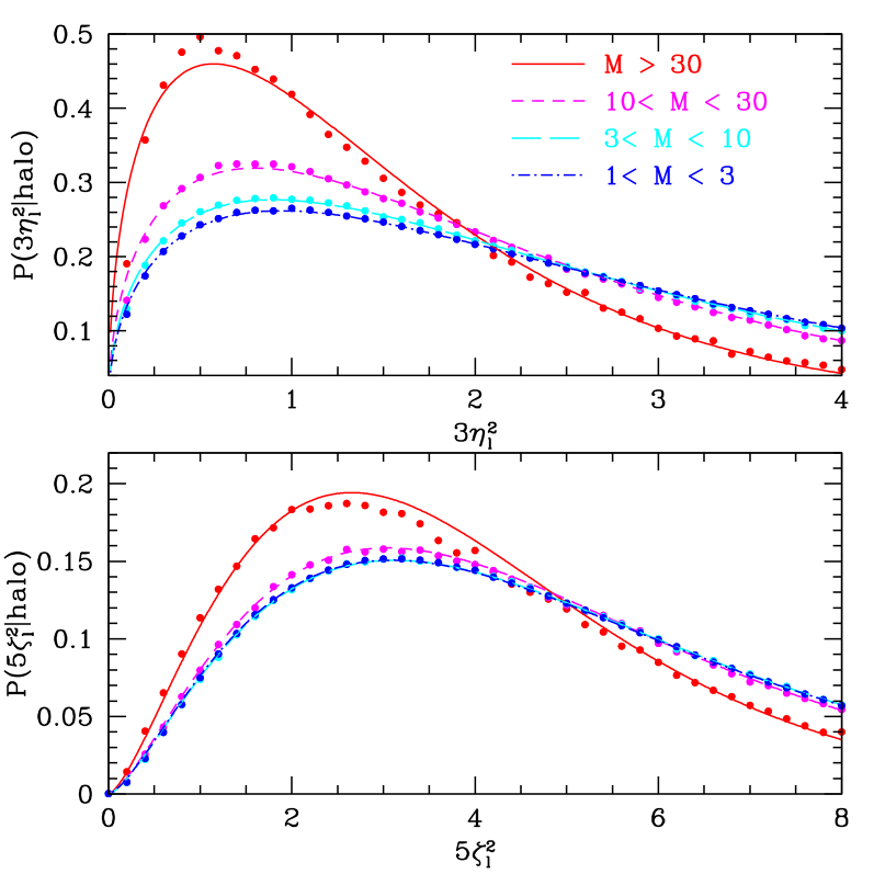
Figure 4: Conditional probability distribution for 3ηl23superscriptsubscript𝜂𝑙23\eta_{l}^{2} (top panel) and 5ζl25superscriptsubscript𝜁𝑙25\zeta_{l}^{2} (bottom panel) measured at the center-of-mass position of proto-halos. The filter is Gaussian with Rl=10h1Mpcsubscript𝑅𝑙10superscript1MpcR_{l}=10\ {\rm{\it h}^{-1}Mpc}. The various curves show the best-fit theoretical predictions for the halo mass bins considered here. Halo mass range are in unit of 1013M/hsuperscript1013subscriptMdirect-product10^{13}\ {\rm M_{\odot}/{\it h}}. Poisson errors are much smaller than the size of the data points and, therefore, do not show up on the figure.

To predict the value of RGsubscript𝑅𝐺R_{G} given RTsubscript𝑅𝑇R_{T}, we followed PSD and assumed that RG(RT)subscript𝑅𝐺subscript𝑅𝑇R_{G}(R_{T}) can be computed through the requirement that δG|δT=δTinner-productsubscript𝛿𝐺subscript𝛿𝑇subscript𝛿𝑇\langle\delta_{G}|\delta_{T}\rangle=\delta_{T}. This yields a prediction for the value of the cross-correlation coefficients ϵ1subscriptitalic-ϵ1\epsilon_{1} and ϵ2subscriptitalic-ϵ2\epsilon_{2} as a function of halo mass, which we can use as an input to χk2(y|x)superscriptsubscript𝜒𝑘2conditional𝑦𝑥\chi_{k}^{2}(y|x) and only fit for x𝑥x. However, we found that using the predicted ϵ1subscriptitalic-ϵ1\epsilon_{1} leads to unphysical (negative) values for x𝑥x when one attempts to fit P(3ηl2|halo)𝑃conditional3superscriptsubscript𝜂𝑙2haloP(3\eta_{l}^{2}|{\rm halo}). Therefore, we decided to proceed as follows:

  1. 1.

    Estimate both ϵ1subscriptitalic-ϵ1\epsilon_{1} and x=3η2|halo𝑥inner-product3superscript𝜂2halox=\langle 3\eta^{2}|{\rm halo}\rangle by fitting the model χ32(y|x;ϵ1)superscriptsubscript𝜒32conditional𝑦𝑥subscriptitalic-ϵ1\chi_{3}^{2}(y|x;\epsilon_{1}) to the measured P(3ηl2|halo)𝑃conditional3superscriptsubscript𝜂𝑙2haloP(3\eta_{l}^{2}|{\rm halo}).

  2. 2.

    Compute ϵ2subscriptitalic-ϵ2\epsilon_{2} assuming that the same RGsubscript𝑅𝐺R_{G} enters the spectral moments.

  3. 3.

    Estimate x=5ζl2|halo𝑥inner-product5superscriptsubscript𝜁𝑙2halox=\langle 5\zeta_{l}^{2}|{\rm halo}\rangle by fitting the theoretical model χ52(y|x;ϵ2)superscriptsubscript𝜒52conditional𝑦𝑥subscriptitalic-ϵ2\chi_{5}^{2}(y|x;\epsilon_{2}) to the simulated P(5ζl2|halo)𝑃conditional5superscriptsubscript𝜁𝑙2haloP(5\zeta_{l}^{2}|{\rm halo}).

We considered data in the range 0<3ηl2<803superscriptsubscript𝜂𝑙280<3\eta_{l}^{2}<8 and 0<5ζl2<1205superscriptsubscript𝜁𝑙2120<5\zeta_{l}^{2}<12 and gave equal weight to all the measurements (assuming Poisson errors does not affect our results significantly). Table 1 summarizes the best-fitting values obtained for four different halo bins spanning the mass range 10131015M/hsuperscript1013superscript1015subscriptMdirect-product10^{13}-10^{15}\ {\rm M_{\odot}/{\it h}}, whereas the measured probability distributions together with the best-fit models are shown in Fig.4. The data is reasonably well described by a conditional χ2superscript𝜒2\chi^{2}-distribution, but the fit is somewhat poorer when the cross-correlation coefficient is close to unity.

Table 1: Best-fit parameter values as a function of halo mass. The latter is in unit of 1013M/hsuperscript1013subscriptMdirect-product10^{13}\ {\rm M_{\odot}/{\it h}}. Note that we also list the values of ϵ2subscriptitalic-ϵ2\epsilon_{2} even though it is not directly fitted to the data (see text for details).
Halo mass 3η2|haloinner-product3superscript𝜂2halo\langle 3\eta^{2}|{\rm halo}\rangle ϵ1subscriptitalic-ϵ1\epsilon_{1} 5ζ2|haloinner-product5superscript𝜁2halo\langle 5\zeta^{2}|{\rm halo}\rangle (ϵ2subscriptitalic-ϵ2\epsilon_{2})
M>30𝑀30M>30 0.71 0.80 2.98 (0.70)
10<M<3010𝑀3010<M<30 1.24 0.66 4.49 (0.52)
3<M<103𝑀103<M<10 1.62 0.54 5.82 (0.37)
1<M<31𝑀31<M<3 1.94 0.49 6.12 (0.31)

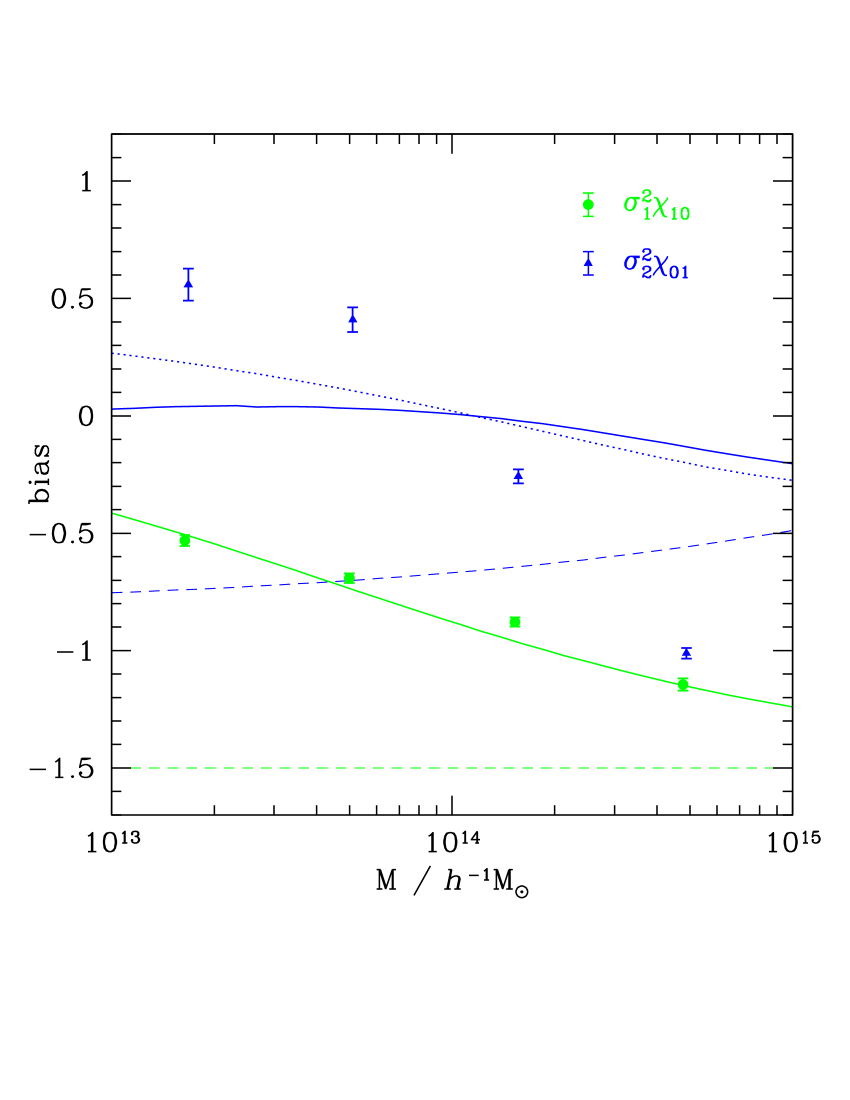
The second-order bias factors χ10subscript𝜒10\chi_{10} and χ01subscript𝜒01\chi_{01} of the dark matter haloes at z=0𝑧0z=0 can be readily computed from Eq.(39) using the best-fit values of 3η2|haloinner-product3superscript𝜂2halo\langle 3\eta^{2}|{\rm halo}\rangle and 5ζ2|haloinner-product5superscript𝜁2halo\langle 5\zeta^{2}|{\rm halo}\rangle. The results are shown in Fig.5 as the data points. Error bars indicate the scatter among the various realizations and, therefore, likely strongly underestimate the true uncertainty. The dashed curves indicate the predictions of the ESP formalism. The measurements, albeit of the same magnitude as the theoretical predictions, quite disagree with expectations based on our ESP approach, especially χ01subscript𝜒01\chi_{01} which reverses sign as the halo mass drops below 1014M/hsuperscript1014subscriptMdirect-product10^{14}\ {\rm M_{\odot}/{\it h}}.

4.3 Interpretation of the measurements

To begin with, we note that, if haloes were forming out of randomly distributed patches in the initial conditions, then both χ10subscript𝜒10\chi_{10} and χ01subscript𝜒01\chi_{01} would be zero since 3η2=3delimited-⟨⟩3superscript𝜂23\langle 3\eta^{2}\rangle=3 and 5ζ2=5delimited-⟨⟩5superscript𝜁25\langle 5\zeta^{2}\rangle=5 for random field points.

The measured dimensionless bias factor σ12χ10superscriptsubscript𝜎12subscript𝜒10\sigma_{1}^{2}\chi_{10} is always negative, which indicates that halos collapse out of regions which have values of η2superscript𝜂2\eta^{2} smaller than average. In our ESP approach, we assume that the center-of-mass position of proto-haloes exactly coincides with that of a local density peak, so that σ12χ103/2superscriptsubscript𝜎12subscript𝜒1032\sigma_{1}^{2}\chi_{10}\equiv-3/2. However, simulations indicate that, while there is a good correspondence between proto-haloes and linear density peaks, the center-of-mass of the former is somewhat offset relative to the peak position (see e.g. Porciani, Dekel & Hoffman, 2002; Ludlow & Porciani, 2011). To model this effect, we note that, if the proto-halo is at a distance R𝑅R from a peak, then the average value of 3η23superscript𝜂23\eta^{2} is 3η2(R)=ϵ12(R)(3η2|pk3)delimited-⟨⟩3superscript𝜂2𝑅superscriptsubscriptitalic-ϵ12𝑅inner-product3superscript𝜂2pk3\bigl{\langle}3\eta^{2}\bigr{\rangle}(R)=\epsilon_{1}^{2}(R)(\bigl{\langle}3\eta^{2}|{\rm pk}\bigr{\rangle}-3) (in analogy with the fact that the average density at a distance R𝑅R from a position where δδc𝛿subscript𝛿𝑐\delta\equiv\delta_{c} is δ(R)=ξδ(R)δcdelimited-⟨⟩𝛿𝑅subscript𝜉𝛿𝑅subscript𝛿𝑐\bigl{\langle}\delta\bigr{\rangle}(R)=\xi_{\delta}(R)\,\delta_{c}). Assuming that the offset R𝑅R follows a Gaussian distribution, the halo bias factor is

σ1s2χ10=322π0dRσ(Rσ)2eR2/2σ2ϵ12(R).superscriptsubscript𝜎1𝑠2subscript𝜒10322𝜋superscriptsubscript0𝑑𝑅𝜎superscript𝑅𝜎2superscript𝑒superscript𝑅22superscript𝜎2superscriptsubscriptitalic-ϵ12𝑅\sigma_{1s}^{2}\chi_{10}=-\frac{3}{2}\sqrt{\frac{2}{\pi}}\int_{0}^{\infty}\!\frac{dR}{\sigma}\left(\frac{R}{\sigma}\right)^{2}e^{-R^{2}/2\sigma^{2}}\epsilon_{1}^{2}(R)\;. (40)

The rms variance σ(M)𝜎𝑀\sigma(M) of the offset distribution, which generally depends on the halo mass, can be constrained from our measurements of χ10subscript𝜒10\chi_{10} for dark matter haloes. The best-fit powerlaw function,

σ(M)=2.50(M1013M/h)0.063h1Mpc,𝜎𝑀2.50superscript𝑀superscript1013subscriptMdirect-product0.063superscript1Mpc\sigma(M)=2.50\left(\frac{M}{10^{13}\ {\rm M_{\odot}/{\it h}}}\right)^{0.063}\ {\rm{\it h}^{-1}Mpc}\;, (41)

turns out to be a weak function of halo mass. In unit of the (tophat) Lagrangian halo radius, this translates into σ/RT0.79𝜎subscript𝑅𝑇0.79\sigma/R_{T}\approx 0.79 and 0.36absent0.36\approx 0.36 for a halo mass M=1013𝑀superscript1013M=10^{13} and 1014M/hsuperscript1014subscriptMdirect-product10^{14}\ {\rm M_{\odot}/{\it h}}, respectively. The resulting theoretical prediction is shown as the solid curve in Fig.5 and agrees reasonably well with our data. This crude approximation demonstrates that an offset between the proto-halo center-of-mass and the peak position can have a large impact on the inferred value of χ10subscript𝜒10\chi_{10}, since the latter is very sensitive to small-scale mass distribution.
Refer to caption
Figure 5: The bias factors σ12χ10superscriptsubscript𝜎12subscript𝜒10\sigma_{1}^{2}\chi_{10} and σ22χ01superscriptsubscript𝜎22subscript𝜒01\sigma_{2}^{2}\chi_{01} of dark matter haloes identified in the N-body simulations at z=0𝑧0z=0 are shown as filled (green) circle and (blue) triangle, respectively. Error bars indicate the scatter among 6 realizations. The horizontal dashed (green) line at 3/232-3/2 and the dashed (blue) curve are the corresponding ESP predictions. The dotted (blue) curve is σ22χ01superscriptsubscript𝜎22subscript𝜒01\sigma_{2}^{2}\chi_{01} in a model where halos are allowed to collapse in filamentary-like structures. The solid curves are our final predictions, which take into account the offset between peak position and proto-halo center-of-mass (see text for details).

Likewise, an offset between the proto-halo center-of-mass and the position of the linear density peak will also impact the measurement of χ01subscript𝜒01\chi_{01}, yet cannot explain the observed sign reversal. In this regard, one should first remember that density peaks become increasingly spherical as ν𝜈\nu\to\infty. Nevertheless, while their mean ellipticity edelimited-⟨⟩𝑒\langle e\rangle and prolateness pdelimited-⟨⟩𝑝\langle p\rangle converge towards zero in this limit, v=uedelimited-⟨⟩𝑣delimited-⟨⟩𝑢𝑒\langle v\rangle=\langle ue\rangle approaches 1/5151/5 at fixed u𝑢u (see Eq.(7.7) of Bardeen et al., 1986). Hence, ζ2=3v2+w2delimited-⟨⟩superscript𝜁2delimited-⟨⟩3superscript𝑣2superscript𝑤2\langle\zeta^{2}\rangle=\langle 3v^{2}+w^{2}\rangle does not tend towards zero but rather unity, like for random field points. Consequently, σ22χ010superscriptsubscript𝜎22subscript𝜒010\sigma_{2}^{2}\chi_{01}\to 0 in the limit ν𝜈\nu\to\infty. Secondly, at any finite ν𝜈\nu, our ESP approach predicts that χ01subscript𝜒01\chi_{01} be negative because we have assumed that proto-haloes only form near a density peak (λ3>0subscript𝜆30\lambda_{3}>0, where λ1λ2λ3subscript𝜆1subscript𝜆2subscript𝜆3\lambda_{1}\geq\lambda_{2}\geq\lambda_{3} are the eigenvalues of ijδsubscript𝑖subscript𝑗𝛿-\partial_{i}\partial_{j}\delta). However, N-body simulations strongly suggest that a fraction of the proto-haloes collapse along the ridges or filaments connecting two density maxima, and that this fraction increases with decreasing halo mass Ludlow & Porciani (2011). To qualitatively assess the impact of such primeval configurations on χ01subscript𝜒01\chi_{01}, we extend the integration domain in the plane (v,w)𝑣𝑤(v,w) to include all the points with λ2>0subscript𝜆20\lambda_{2}>0 and λ3<0subscript𝜆30\lambda_{3}<0 (but still require that the curvature u𝑢u be positive). This way we not only consider density peaks, but also extrema that correspond to filamentary configurations. The resulting curvature function f(u,α)𝑓𝑢𝛼f(u,\alpha) can be cast into the compact form

f(u,α)𝑓𝑢𝛼\displaystyle f(u,\alpha) =1α4{e5αu2210π(αu2165)\displaystyle=\frac{1}{\alpha^{4}}\Biggl{\{}\frac{e^{-{5\alpha u^{2}\over 2}}}{\sqrt{10\pi}}\left(\alpha u^{2}-\frac{16}{5}\right) (42)
+e5αu2810π(31αu2+325)+α2(αu33u)superscript𝑒5𝛼superscript𝑢2810𝜋31𝛼superscript𝑢2325𝛼2𝛼superscript𝑢33𝑢\displaystyle\quad+\frac{e^{-{5\alpha u^{2}\over 8}}}{\sqrt{10\pi}}\left(31\alpha u^{2}+\frac{32}{5}\right)+\frac{\sqrt{\alpha}}{2}\left(\alpha u^{3}-3u\right)
×[Erf(5α2u2)+Erf(5α2u)1]},\displaystyle\qquad\times\left[{\rm Erf}\left(\sqrt{\frac{5\alpha}{2}}\frac{u}{2}\right)+{\rm Erf}\left(\sqrt{\frac{5\alpha}{2}}u\right)-1\right]\Biggr{\}}\;,

The dotted curve in Fig.5 shows σ22χ01superscriptsubscript𝜎22subscript𝜒01\sigma_{2}^{2}\chi_{01} when the filamentary configurations are included. While it agrees with the original ESP prediction at large halo mass, it reverses sign around 1014M/hsuperscript1014subscriptMdirect-product10^{14}\ {\rm M_{\odot}/{\it h}} because, as the peak height decreases, configurations with λ3<0subscript𝜆30\lambda_{3}<0 or, equivalently, large values of ζ2superscript𝜁2\zeta^{2} become more probable. The solid curve takes into account, in addition to filamentary configurations, an offset between the proto-halo and the peak position according to the simple prescription discussed above. This is our final prediction for σ22χ01superscriptsubscript𝜎22subscript𝜒01\sigma_{2}^{2}\chi_{01}. It is clearly at odds with the measurements, which strongly suggest that σ22χ01superscriptsubscript𝜎22subscript𝜒01\sigma_{2}^{2}\chi_{01} can be very different from zero for M1013M/hgreater-than-or-equivalent-to𝑀superscript1013subscriptMdirect-productM\gtrsim 10^{13}\ {\rm M_{\odot}/{\it h}}.

It is beyond the scope of this paper to work out a detailed description of the measurements. Using a value of RGsubscript𝑅𝐺R_{G} different than that obtained through the condition δG|δT=δTinner-productsubscript𝛿𝐺subscript𝛿𝑇subscript𝛿𝑇\langle\delta_{G}|\delta_{T}\rangle=\delta_{T} has a large impact on the mass function, suggesting that it will be difficult to get a good fit of both the mass function and the bias factors χ10subscript𝜒10\chi_{10} and χ01subscript𝜒01\chi_{01}. Before concluding however, we note that, if the Lagrangian clustering of haloes also depends on s2(𝐱)=sij(𝐱)sij(𝐱)subscript𝑠2𝐱subscript𝑠𝑖𝑗𝐱superscript𝑠𝑖𝑗𝐱s_{2}(\mathrm{\bf x})=s_{ij}(\mathrm{\bf x})s^{ij}(\mathrm{\bf x}), where (in suitable units)

sij(𝐱)=ijϕ(𝐱)13δijδ(𝐱),subscript𝑠𝑖𝑗𝐱subscript𝑖subscript𝑗italic-ϕ𝐱13subscript𝛿𝑖𝑗𝛿𝐱s_{ij}(\mathrm{\bf x})=\partial_{i}\partial_{j}\phi(\mathrm{\bf x})-\frac{1}{3}\delta_{ij}\delta(\mathrm{\bf x})\;, (43)

then we are not measuring χ01subscript𝜒01\chi_{01} but some weighted and scale-dependent combination of both χ01subscript𝜒01\chi_{01} and the Lagrangian bias γ2subscript𝛾2\gamma_{2} associated with s2(𝐱)subscript𝑠2𝐱s_{2}(\mathrm{\bf x}). Recent numerical work indeed suggests that γ2subscript𝛾2\gamma_{2} might be non-zero for massive haloes (Baldauf et al., 2012; Chan, Scoccimarro & Sheth, 2012; Sheth, Chan & Scoccimarro, 2013). In this regards, our approach can furnish a useful cross-check of these results since it can provide a measurement of γ2subscript𝛾2\gamma_{2} which is independent of the bispectrum.

5 Conclusion

Dark matter haloes and galaxies are inherently biased relative to the mass density field, and this bias can manifest itself not only in n𝑛n-point statistics such as the power spectrum or bispectrum, but also in simpler one-point statistics. In this work, we took advantage of this to ascertain the importance of certain nonlocal Lagrangian bias factors independently of a 2-point measurement. We extended the cross-correlation technique of Musso, Paranjape & Sheth (2012) to χ2superscript𝜒2\chi^{2}-distributed variables, focusing on the quadratic terms η2(𝐱)superscript𝜂2𝐱\eta^{2}(\mathrm{\bf x}) and ζ2(𝐱)superscript𝜁2𝐱\zeta^{2}(\mathrm{\bf x}) (see Eq.20) which arise from the peak constraint and for which we have theoretical predictions. In principle however, our approach could be applied to measure the Lagrangian bias factor associated with any χ2superscript𝜒2\chi^{2}-distributed variable such as the tidal shear for instance. We validated our method with peaks of Gaussian random field before applying it to a catalogue of dark matter haloes with mass M>1013M/h𝑀superscript1013subscriptMdirect-productM>10^{13}\ {\rm M_{\odot}/{\it h}}. Including an offset between the proto-halo center-of-mass and the peak position in the modelling (motivated by the analysis of Ludlow & Porciani, 2011), we were able to reproduce our measurements of the nonlocal bias σ12χ10superscriptsubscript𝜎12subscript𝜒10\sigma_{1}^{2}\chi_{10}. Our result χ10<0subscript𝜒100\chi_{10}<0 is consistent with the findings of Ludlow & Porciani (2011), who demonstrated that proto-haloes with M>1013M/h𝑀superscript1013subscriptMdirect-productM>10^{13}\ {\rm M_{\odot}/{\it h}} preferentially form near initial density peaks (χ100subscript𝜒100\chi_{10}\equiv 0 for a random distribution). However, we were unable to explain the measurements of σ22χ01superscriptsubscript𝜎22subscript𝜒01\sigma_{2}^{2}\chi_{01}, even with the additional assumption that a fraction of the haloes collapse from filamentary-like structures rather than density peaks. We speculate that a dependence of the halo Lagrangian bias on s2(𝐱)subscript𝑠2𝐱s_{2}({\bf x}) might be needed to explain this discrepancy.

The dependence on η2(𝐱)superscript𝜂2𝐱\eta^{2}({\bf x}) induces a correction 2χ10(𝐤1𝐤2)2subscript𝜒10subscript𝐤1subscript𝐤2-2\chi_{10}(\mathrm{\bf k}_{1}\cdot\mathrm{\bf k}_{2}) to the halo bias which, for collinear wavevectors 𝐤1subscript𝐤1\mathrm{\bf k}_{1} and 𝐤2subscript𝐤2\mathrm{\bf k}_{2} of wavenumber 0.1h1Mpc0.1superscript1Mpc0.1\ {\rm{\it h}^{-1}Mpc}, is Δb0.02Δ𝑏0.02\Delta b\approx 0.02 (0.05) and 0.30absent0.30\approx 0.30 (0.88) for haloes of mass M=1013𝑀superscript1013M=10^{13} and 1014M/hsuperscript1014subscriptMdirect-product10^{14}\ {\rm M_{\odot}/{\it h}} at redshift z=0𝑧0z=0 (z=1), respectively. Relative to the evolved, linear halo bias b1E1+b100superscriptsubscript𝑏1E1subscript𝑏100b_{1}^{\rm E}\equiv 1+b_{100}, the fractional correction is Δb/b1Esimilar-toΔ𝑏superscriptsubscript𝑏1Eabsent\Delta b/b_{1}^{\rm E}\sim2% and 15similar-toabsent15\sim 15% for the same low and high halo mass in the redshift range 0<z<10𝑧10<z<1. Hence, this correction can safely be ignored for M=1013h1Mpc𝑀superscript1013superscript1MpcM=10^{13}\ {\rm{\it h}^{-1}Mpc}, but it could become relevant at larger halo masses.

We also refined the ESP approach of PSD so that clustering statistics can be straightforwardly computed from the (effective) bias expansion Eq.(19) (following the prescription detailed in Desjacques, 2013). We checked that the predicted halo mass function, from which all the bias factors can be derived, agrees well with the numerical data. However, some of the model ingredients, especially the filtering of the density field, will have to be better understood if one wants to make predictions that are also accurate at small scales.

Acknowledgment

V.D. would like to thank the Perimeter Institute for Theoretical Physics and CCPP at New York University for their hospitality while some of this work was being completed there. M.B., K.C.C. and V.D. acknowledge support by the Swiss National Science Foundation.

References

  • Baldauf et al. (2012) Baldauf T., Seljak U., Desjacques V., McDonald P., 2012, Phys. Rev. D, 86, 083540
  • Bardeen et al. (1986) Bardeen J. M., Bond J. R., Kaiser N., Szalay A. S., 1986, Astrophys. J., 304, 15
  • Barkana (2004) Barkana R., 2004, Mon. Not. R. Astron. Soc., 347, 59
  • Bernardeau et al. (2002) Bernardeau F., Colombi S., Gaztañaga E., Scoccimarro R., 2002, Phys. Rep., 367, 1
  • Bond (1989) Bond J. R., 1989, in Frontiers in Physics - From colliders to cosmology, proceedings of the Lake Louise Winter Institute, Astbury A., Campbell B., Israel W., Kamal A., Khanna F., eds., pp. 182–235
  • Bond et al. (1991) Bond J. R., Cole S., Efstathiou G., Kaiser N., 1991, Astrophys. J., 379, 440
  • Catelan, Matarrese & Porciani (1998) Catelan P., Matarrese S., Porciani C., 1998, Astrophys. J. Lett., 502, L1
  • Chan, Scoccimarro & Sheth (2012) Chan K. C., Scoccimarro R., Sheth R. K., 2012, Phys. Rev. D, 85, 083509
  • Crocce, Pueblas & Scoccimarro (2006) Crocce M., Pueblas S., Scoccimarro R., 2006, Mon. Not. R. Astron. Soc., 373, 369
  • Dalal et al. (2008) Dalal N., White M., Bond J. R., Shirokov A., 2008, Astrophys. J., 687, 12
  • Desjacques (2013) Desjacques V., 2013, Phys. Rev. D, 87, 043505
  • Desjacques et al. (2010) Desjacques V., Crocce M., Scoccimarro R., Sheth R. K., 2010, Phys. Rev. D, 82, 103529
  • Desjacques, Gong & Riotto (2013) Desjacques V., Gong J.-O., Riotto A., 2013, JCAP , 9, 6
  • Elia, Ludlow & Porciani (2011) Elia A., Ludlow A. D., Porciani C., 2011
  • Ferraro et al. (2012) Ferraro S., Smith K. M., Green D., Baumann D., 2012, ArXiv e-prints: 1209.2175
  • Fry & Gaztanaga (1993) Fry J. N., Gaztanaga E., 1993, Astrophys. J., 413, 447
  • Gradshteyn & Ryzhik (1994) Gradshteyn I. S., Ryzhik I. M., 1994, Table of integrals, series and products. New York: Academic Press, —c1994, 5th ed. completely reset, edited by Jeffrey, Alan
  • Gunst & Webster (1973) Gunst R. F., Webster J. T., 1973, J. Stat. Comput. Sim., 2, 275
  • Hahn & Paranjape (2014) Hahn O., Paranjape A., 2014, Mon. Not. R. Astron. Soc., 438, 878
  • Kaiser (1984) Kaiser N., 1984, Astrophys. J. Lett., 284, L9
  • Knollmann & Knebe (2009) Knollmann S. R., Knebe A., 2009, Astrophys. J. Supp., 182, 608
  • Komatsu et al. (2011) Komatsu E. et al., 2011, Astrophys. J. Supp., 192, 18
  • Lewis, Challinor & Lasenby (2000) Lewis A., Challinor A., Lasenby A., 2000, Astrophys. J., 538, 473
  • Ludlow & Porciani (2011) Ludlow A. D., Porciani C., 2011, Mon. Not. R. Astron. Soc., 413, 1961
  • Maggiore & Riotto (2010) Maggiore M., Riotto A., 2010, Astrophys. J., 717, 515
  • Matsubara (2012) Matsubara T., 2012, Phys. Rev. D, 86, 063518
  • McDonald & Roy (2009) McDonald P., Roy A., 2009, JCAP , 8, 20
  • Musso, Paranjape & Sheth (2012) Musso M., Paranjape A., Sheth R. K., 2012, Mon. Not. R. Astron. Soc., 427, 3145
  • Musso & Sheth (2012) Musso M., Sheth R. K., 2012, Mon. Not. R. Astron. Soc., 423, L102
  • Paranjape et al. (2013) Paranjape A., Sefusatti E., Chan K. C., Desjacques V., Monaco P., Sheth R. K., 2013, ArXiv e-prints: 1305.5830
  • Paranjape & Sheth (2012) Paranjape A., Sheth R. K., 2012, Mon. Not. R. Astron. Soc., 426, 2789
  • Paranjape, Sheth & Desjacques (2013) Paranjape A., Sheth R. K., Desjacques V., 2013, Mon. Not. R. Astron. Soc., 431, 1503
  • Porciani, Dekel & Hoffman (2002) Porciani C., Dekel A., Hoffman Y., 2002, Mon. Not. R. Astron. Soc., 332, 339
  • Robertson et al. (2009) Robertson B. E., Kravtsov A. V., Tinker J., Zentner A. R., 2009, Astrophys. J., 696, 636
  • Sheth, Chan & Scoccimarro (2013) Sheth R. K., Chan K. C., Scoccimarro R., 2013, Phys. Rev. D, 87, 083002
  • Sheth, Mo & Tormen (2001) Sheth R. K., Mo H. J., Tormen G., 2001, Mon. Not. R. Astron. Soc., 323, 1
  • Springel (2005) Springel V., 2005, Mon. Not. R. Astron. Soc., 364, 1105
  • Tiku (1965) Tiku M. L., 1965, Biometrika, 52, 415
  • Tinker et al. (2008) Tinker J., Kravtsov A. V., Klypin A., Abazajian K., Warren M., Yepes G., Gottlöber S., Holz D. E., 2008, Astrophys. J., 688, 709
  • Valageas (2009) Valageas P., 2009, Astron. Astrophys., 508, 93

Appendix A The curvature function of density peaks

The curvature function of density peaks is (Bardeen et al., 1986)

f(u,α)𝑓𝑢𝛼\displaystyle f(u,\alpha) =1α4{e5αu2210π(αu2165)\displaystyle=\frac{1}{\alpha^{4}}\Biggl{\{}\frac{e^{-{5\alpha u^{2}\over 2}}}{\sqrt{10\pi}}\left(\alpha u^{2}-\frac{16}{5}\right) (44)
+e5αu2810π(312αu2+165)+α2(αu33u)superscript𝑒5𝛼superscript𝑢2810𝜋312𝛼superscript𝑢2165𝛼2𝛼superscript𝑢33𝑢\displaystyle\quad+\frac{e^{-{5\alpha u^{2}\over 8}}}{\sqrt{10\pi}}\left(\frac{31}{2}\alpha u^{2}+\frac{16}{5}\right)+\frac{\sqrt{\alpha}}{2}\left(\alpha u^{3}-3u\right)
×[Erf(5α2u2)+Erf(5α2u)]}.\displaystyle\qquad\times\left[{\rm Erf}\left(\sqrt{\frac{5\alpha}{2}}\frac{u}{2}\right)+{\rm Erf}\left(\sqrt{\frac{5\alpha}{2}}u\right)\right]\Biggr{\}}\;.

Note that Desjacques et al. (2010) introduced the extra variable α𝛼\alpha in order to get a closed form expression for their 2-point peak correlation, while Desjacques (2013) showed that α1𝛼1\alpha\neq 1 can be interpreted as a long-wavelength perturbation in ζ2(𝐱)superscript𝜁2𝐱\zeta^{2}(\mathrm{\bf x}).

Refer to caption
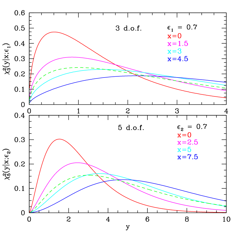
Figure 6: Conditional chi-squared distribution χk2(y|x;ϵ)superscriptsubscript𝜒𝑘2conditional𝑦𝑥italic-ϵ\chi_{k}^{2}(y|x;\epsilon) for 3 and 5 degrees of freedom. Results are shown for several values of x𝑥x and a fixed cross-correlation coefficient ϵ=0.7italic-ϵ0.7\epsilon=0.7. The dashed (green) curve represents the unconditional distribution χk2(y)superscriptsubscript𝜒𝑘2𝑦\chi_{k}^{2}(y).

Appendix B Bivariate χ2superscript𝜒2\chi^{2} distributions

We take the following expression for the bivariate χ2superscript𝜒2\chi^{2}-distribution (Gunst & Webster, 1973)

χk2(x,y;ϵ)subscriptsuperscript𝜒2𝑘𝑥𝑦italic-ϵ\displaystyle\chi^{2}_{k}(x,y;\epsilon) =(xy)k/212kΓ2(k/2)(1ϵ2)k/2ex+y2(1ϵ2)absentsuperscript𝑥𝑦𝑘21superscript2𝑘superscriptΓ2𝑘2superscript1superscriptitalic-ϵ2𝑘2superscript𝑒𝑥𝑦21superscriptitalic-ϵ2\displaystyle=\frac{(xy)^{k/2-1}}{2^{k}\Gamma^{2}(k/2)}\left(1-\epsilon^{2}\right)^{-k/2}e^{-\frac{x+y}{2(1-\epsilon^{2})}} (45)
×F10(k2;ϵ2xy4(1ϵ2)2),absentsubscriptsubscript𝐹10𝑘2superscriptitalic-ϵ2𝑥𝑦4superscript1superscriptitalic-ϵ22\displaystyle\qquad\times{}_{0}F_{1}\!\left(\frac{k}{2};\frac{\epsilon^{2}xy}{4(1-\epsilon^{2})^{2}}\right)\;,

where x𝑥x and y𝑦y are distributed as χ2superscript𝜒2\chi^{2}-variables with k𝑘k d.o.f., ϵ21superscriptitalic-ϵ21\epsilon^{2}\leq 1 is their correlation and F10subscriptsubscript𝐹10{}_{0}F_{1} is a confluent hypergeometric function. On using the fact that modified Bessel functions of the first kind can be written as Iα(x)=iαJα(ix)subscript𝐼𝛼𝑥superscript𝑖𝛼subscript𝐽𝛼𝑖𝑥I_{\alpha}(x)=i^{-\alpha}J_{\alpha}(ix), where

Jα(x)=(x/2)αΓ(α+1)F10(α+1;x24),subscript𝐽𝛼𝑥superscript𝑥2𝛼Γ𝛼1subscriptsubscript𝐹10𝛼1superscript𝑥24J_{\alpha}(x)=\frac{(x/2)^{\alpha}}{\Gamma(\alpha+1)}\,{}_{0}F_{1}(\alpha+1;-\frac{x^{2}}{4})\;, (46)

the bivariate χ2superscript𝜒2\chi^{2}-distribution can be reorganized into the product

χk2(x,y;ϵ)=χk2(x)χk2(y|x;ϵ),subscriptsuperscript𝜒2𝑘𝑥𝑦italic-ϵsubscriptsuperscript𝜒2𝑘𝑥subscriptsuperscript𝜒2𝑘conditional𝑦𝑥italic-ϵ\chi^{2}_{k}(x,y;\epsilon)=\chi^{2}_{k}(x)\chi^{2}_{k}(y|x;\epsilon)\;, (47)

where

χk2(y|x;ϵ)=ey+ϵ2x2(1ϵ2)2(1ϵ2)(yϵ2x)α/2Iα(ϵxy1ϵ2),subscriptsuperscript𝜒2𝑘conditional𝑦𝑥italic-ϵsuperscript𝑒𝑦superscriptitalic-ϵ2𝑥21superscriptitalic-ϵ221superscriptitalic-ϵ2superscript𝑦superscriptitalic-ϵ2𝑥𝛼2subscript𝐼𝛼italic-ϵ𝑥𝑦1superscriptitalic-ϵ2\chi^{2}_{k}(y|x;\epsilon)=\frac{e^{-\frac{y+\epsilon^{2}x}{2(1-\epsilon^{2})}}}{2(1-\epsilon^{2})}\left(\frac{y}{\epsilon^{2}x}\right)^{\alpha/2}I_{\alpha}\!\left(\frac{\epsilon\sqrt{xy}}{1-\epsilon^{2}}\right)\;, (48)

and α=k/21𝛼𝑘21\alpha=k/2-1. This conditional distribution takes a form similar to that of a non-central χ2superscript𝜒2\chi^{2}-distribution χk2(x;λ)subscriptsuperscript𝜒superscript2𝑘𝑥𝜆\chi^{2^{\prime}}_{k}(x;\lambda), where λ𝜆\lambda is the non-centrality parameter. Fig.6 displays χk2(y|x;ϵ)superscriptsubscript𝜒𝑘2conditional𝑦𝑥italic-ϵ\chi_{k}^{2}(y|x;\epsilon) for several values of x𝑥x, assuming k=3𝑘3k=3 and 5. Note that χk2(y|x=k;ϵ)superscriptsubscript𝜒𝑘2conditional𝑦𝑥𝑘italic-ϵ\chi_{k}^{2}(y|x=k;\epsilon) is different from χk2(y)superscriptsubscript𝜒𝑘2𝑦\chi_{k}^{2}(y).

Using the series expansion of χk2(x;λ)subscriptsuperscript𝜒superscript2𝑘𝑥𝜆\chi^{2^{\prime}}_{k}(x;\lambda) in terms of Laguerre polynomials (Tiku, 1965), we arrive at

χk2(y|x;ϵ)superscriptsubscript𝜒𝑘2conditional𝑦𝑥italic-ϵ\displaystyle\chi_{k}^{2}(y|x;\epsilon) =ey2(1ϵ2)2(1ϵ2)α+1(y2)αabsentsuperscript𝑒𝑦21superscriptitalic-ϵ22superscript1superscriptitalic-ϵ2𝛼1superscript𝑦2𝛼\displaystyle=\frac{e^{-\frac{y}{2(1-\epsilon^{2})}}}{2(1-\epsilon^{2})^{\alpha+1}}\left(\frac{y}{2}\right)^{\alpha} (49)
×j=0(ϵ21ϵ2)jΓ(12k+j)(x2)jLj(α)[y2(1ϵ2)].\displaystyle\qquad\times\sum_{j=0}^{\infty}\frac{\left(\frac{-\epsilon^{2}}{1-\epsilon^{2}}\right)^{j}}{\Gamma\left(\frac{1}{2}k+j\right)}\left(\frac{x}{2}\right)^{j}L_{j}^{(\alpha)}\!\!\left[\frac{y}{2(1-\epsilon^{2})}\right]\;.

This series expansion is used to obtain the right-hand side of Eq.(26).