Abstract

Quantum electrodynamics and electroweak corrections are important ingredients for many theoretical predictions at the LHC. This paper documents APFEL, a new PDF evolution package that allows for the first time to perform DGLAP evolution up to NNLO in QCD and to LO in QED, in the variable-flavor-number scheme and with either pole or $\overline{\mathrm{MS}}$ heavy quark masses. APFEL consistently accounts for the QED corrections to the evolution of quark and gluon PDFs and for the contribution from the photon PDF in the proton. The coupled QCD$\otimes$QED equations are solved in $x$-space by means of higher order interpolation, followed by Runge-Kutta solution of the resulting discretized evolution equations. APFEL is based on an innovative and flexible methodology for the sequential solution of the QCD and QED evolution equations and their combination. In addition to PDF evolution, APFEL provides a module that computes Deep-Inelastic Scattering structure functions in the FONLL general-mass variable-flavor-number scheme up to $\mathcal{O}\left(\alpha_{s}^{2}\right)$. All the functionalities of APFEL can be accessed via a Graphical User Interface, supplemented with a variety of plotting tools for PDFs, parton luminosities and structure functions. Written in Fortran 77, APFEL can also be used via the C/C++ and Python interfaces, and is publicly available from the HepForge repository.

Program Summary

Name of the program: APFEL
Version: 2.0.0
Program obtainable from: http://projects.hepforge.org/apfel/
Distribution format: compressed tar file and directly from the HepForge svn repository
E-mail: valerio.bertone@cern.ch, stefano.carrazza@mi.infn.it  and juan.rojo@cern.ch
License: GNU Public License
Computers: all
Operating systems: all
Program language: Fortran 77, C/C++ and Python
Memory required to execute: $\lesssim$ 2 MB
Other programs called: LHAPDF
External files needed: none
Number of bytes in distributed program, including test data etc.: $\sim 2.4$ MB
Keywords: unpolarised parton distribution functions (PDFs), DGLAP evolution equations, QED corrections, electroweak effects, deep-inelastic scattering (DIS).
Nature of the physical problem: Solution of the unpolarized coupled DGLAP evolution equations up to NNLO in QCD and to LO in QED in the variable-flavor-number scheme, both with pole and with $\overline{\mathrm{MS}}$ masses.
Method of solution: Representation of parton distributions and splitting functions on a grid in $x$, discretization of DGLAP evolution equations and higher-order interpolation for general values of $x$, numerical solution of the resulting discretized evolution equations using Runge-Kutta methods.
Restrictions on complexity of the problem: Smoothness of the initial conditions for the PDF evolution.
Typical running time: a few seconds for initialisation, then $\sim$0.5 s for the generation of the PDF tables with combined QCD$\otimes$QED evolution (on a Intel(R) Core(TM)2 Duo CPU E6750 @ 2.66GHz).

1 Introduction

The requirements of precision physics at the LHC demand parton distribution functions (PDFs) that are determined using NLO and NNLO QCD theory (see [1, 2, 3] for recent reviews). For a substantial number of processes, the accuracy in both theoretical predictions and experimental data is such that Quantum Electrodynamics (QED) and pure electroweak corrections also need to be included. Predictions for hadron-collider processes that include QED and electroweak corrections are available for inclusive $W$ and $Z$ production [4, 5, 6, 7, 8, 9, 10, 11, 12, 13, 14], $W$ and $Z$ boson production in association with jets [15, 16, 17], diboson production [18, 19, 20], dijet production [21, 22] and top quark pair production [23, 24, 25, 26, 27] among others, see also Ref. [28] for a recent review.

In order to derive consistent predictions for hadronic cross-sections, both hard-scattering matrix elements and PDFs need to be determined with the same accuracy in the QCD and electroweak couplings. In particular, combining QCD and electroweak calculations at hadron colliders requires parton distributions that have been determined using the coupled QCD$\otimes$QED DGLAP evolution equations [29, 30, 31]. Until recently, the only PDF set which included QED corrections was the MRST04QED set, presented almost ten years ago [32]. Recently, the NNPDF2.3QED set [33, 34, 35] has also become available: on top of providing an up-to-date PDF set determined using LO/NLO/NNLO QCD supplemented by LO QED theory, for the first time the photon PDF, with the corresponding uncertainty, has been extracted from LHC measurements on electroweak gauge boson production, rather than being based on model assumptions.

While much work has been devoted to the study of numerical solutions of the QCD DGLAP evolution equations and their implementation in public tools [39, 40, 41, 42, 43, 44, 45, 46], less effort has been devoted to the solutions of the DGLAP equations in the presence of QED corrections [47, 48, 32]. To the best of our knowledge, the only public code which offers such possibility is partonevolution [49, 48]. However, partonevolution is limited to NLO QCD corrections and in addition it does not allow to explore different possibilities for the combination of the QCD and QED evolution equations.

Therefore, the main motivation for this work is to provide for the first time a public code, accurate and flexible, that can be used to perform PDF evolution up to NNLO in QCD and LO in QED, both in the fixed-flavour-number (FFN) and in the variable-flavour-number (VFN) schemes, and using either pole or $\overline{\mathrm{MS}}$ heavy quark masses. Another motivation was to complete the discussion about the solutions of the QCD$\otimes$QED combined equations that was only sketched in the original NNPDF2.3QED publication [33], as well as to provide another independent validation of the FastKernel implementation used in the determination of those PDF sets.

We call this code APFEL, which stands for A Parton distribution Function Evolution Library. APFEL is based on an innovative methodology for the solution of the QCD and QED evolution equations and their combination, leading to a flexibility that can be used to explore various options that differ by subleading terms. APFEL solves the QCD$\otimes$QED equations sequentially, that is, first performing QCD evolution and then QED evolution, or vice-versa. The particular ordering, as well as the related choices to be made when crossing heavy quark thresholds, can be easily modified by the user. These various possibilities differ only by subleading terms, that can however lead to a phenomenological impact, so it is important to quantify these in some detail.

Public codes for the evolution of parton distributions and fragmentation functions can be divided according to the method they use to solve the DGLAP equations. A first family consists of $x$-space methods, which typically use a representation of the PDFs on a grid in $x$ together with higher-order interpolation techniques for the solution of the intergro-differential equations [39, 41, 43, 44, 42]. The widely used HOPPET [39] and QCDNUM [41] programs belong to this family. The other family is composed of $N$-space codes, where the DGLAP equations are first transformed into Mellin space, analytically solved, and then inverted back to $x$-space using complex-variable methods [45, 40, 49, 48, 46]. The PEGASUS [45] program is one of the best-known examples of this strategy. The main drawback of the $N$-space methods, however, is the fact that they require the analytical Mellin transform of the initial PDFs which is possible only for some very specific functional forms. A third approach is provided by the hybrid method adopted in the FastKernel program, the internal code used in the NNPDF fits [50, 51], where the DGLAP equations are solved in Mellin space and then used to determine the $x$-space evolution operators, which are convoluted with the $x$-space PDFs to perform the evolution.

Inspired in part by the techniques used in the HOPPET and QCDNUM programs, APFEL solves the QCD$\otimes$QED evolution equations in $x$-space by means of higher-order interpolation, followed by Runge-Kutta solution of the resulting discretized evolution equations. Its main strength is that, on top of providing fast and efficient state-of-the-art QCD evolution, it allows to use the variable-flavour-number scheme in the QED evolution of PDFs and to systematically explore a range of possible options to solve the combined evolution equations. For these reasons, we believe that APFEL has the potential to become an important tool for the present and coming generation of PDF analyses including QED corrections.

On top of the PDF evolution routines, APFEL includes also two additional modules that should be of interest for a variety of users. The first one allows the computation of neutral- and charged-current Deep-Inelastic Scattering (DIS) structure functions up to $\mathcal{O}\left(\alpha_{s}^{2}\right)$ in the FONLL general-mass VFN scheme [52] as well as in the zero-mass VFN and FFN schemes [53]. The second is a user-friendly, flexible Graphical User Interface (GUI), which provides easy access to all the functionalities of APFEL, and that is supplemented with a variety of graphical plotting tools for PDFs, parton luminosities and structure functions.

The outline of this paper is the following. In Sect. 2 we review the structure of the coupled QCD$\otimes$QED evolution equations and discuss their solution and the different options for the treatment of subleading terms, and we also briefly discuss the implementation deep-inelastic structure functions. In Sect. 3 we describe the numerical techniques that are used in APFEL. Then in Sect. 4 we introduce the main functionalities of APFEL and describe the standard user interface, as well as the Graphical User Interface which provides a user-friendly interface to all these functionalities and to a variety of plotting tools. In Sect. 5 we validate APFEL by benchmarking it against other publicly available tools, and finally in Sect. 6 we conclude and discuss possible future developments.

2 DGLAP evolution with QED corrections

In this section we present the strategy that APFEL adopts in order to perform the DGLAP evolution of parton distributions when both QCD and QED effects are taken into account. First of all, we will present the method used to solve the QED evolution equations, then how to combine the QCD and QED solutions, and finally the treatment of heavy quark thresholds in the variable-flavor-number scheme. QCD corrections to the DGLAP evolution equations [54, 55, 56] are available up to NNLO [57, 58, 59, 60, 61, 62, 63, 64], and the structure of their solutions has been discussed in great detail in the literature, see for instance [39, 45, 1] and references therein. In this section we limit ourselves to discussing only the new features that arise in the DGLAP equations when QED effects are taken into account. Finally, in the last subsection we briefly review the theory of Deep-Inelastic Scattering structure functions.

2.1 Solving the QED evolution equations

The implementation of the QED corrections to the DGLAP evolution equations leads to the inclusion of additional terms which contain QED splitting functions [29, 30, 31], proportional to the QED coupling $\alpha$, convoluted with the PDFs. There are several possibilities to solve the coupled QCD$\otimes$QED DGLAP evolution equations, and, as opposed to previous works, APFEL adopts a fully factorized approach. In this approach, the QCD and the QED factorization procedures can be regarded as two independent steps that lead to two independent factorization scales, on which all PDFs depend, denoted by $\mu$ for QCD and $\nu$ for QED, that is, $q_{i}\equiv q_{i}(x,\mu,\nu)$.

In the particular case where QED corrections are included up to $\mathcal{O}(\alpha)$ and the mixed subleading terms $\mathcal{O}(\alpha\alpha_{s})$ are neglected, the QCD evolution with respect to $\mu$ and the QED evolution with respect to $\nu$ will be given by two fully decoupled equations:

$$\begin{array}[]{rcl}\displaystyle\mu^{2}{{\partial}\over{\partial\mu^{2}}}{\mathbf{q}}(x,\mu,\nu)&=&\displaystyle{\mathbf{P}}^{\rm QCD}(x,\alpha_{s}(\mu))\otimes{\mathbf{q}}(x,\mu,\nu)\,,\\ \\ \displaystyle\nu^{2}{{\partial}\over{\partial\nu^{2}}}{\mathbf{q}}(x,\mu,\nu)&=&\displaystyle{\mathbf{P}}^{\rm QED}(x,\alpha(\nu))\otimes{\mathbf{q}}(x,\mu,\nu)\,,\end{array}$$ (1)

where ${\mathbf{P}}^{\rm QCD}$ and ${\mathbf{P}}^{\rm QED}$ are respectively the QCD and QED matrices of splitting functions and ${\mathbf{q}}(x,\mu,\nu)$ is a vector containing all the parton distribution functions. Let us recall that in the presence of QED corrections, the photon PDF $\gamma(x,\mu,\nu)$ should also be included in ${\mathbf{q}}(x,\mu,\nu)$. The symbol $\otimes$ in Eq. (1) represents the usual convolution operator defined as:

$$A(x)\otimes B(x)\equiv\int_{0}^{1}dy\int_{0}^{1}dz\,A(y)B(z)\delta(x-yz)\,.$$ (2)

The independent solutions of the differential equations in Eq. (1), irrespective of the numerical technique used, will give as a result two different evolution operators: ${\bm{\Gamma}}^{\rm QCD}$, that evolves the array $\mathbf{q}$ in $\mu$ while keeping $\nu$ constant, and ${\bm{\Gamma}}^{\rm QED}$, that evolves $\mathbf{q}$ in $\nu$ while keeping $\mu$ constant. If the QCD evolution takes place between $\mu_{0}$ and $\mu_{1}$ and the QED evolution between $\nu_{0}$ and $\nu_{1}$, we will have that:

$$\begin{array}[]{l}\displaystyle{\mathbf{q}}(x,\mu_{1},\nu)={\bm{\Gamma}}^{\rm QCD}(x|\mu_{1},\mu_{0})\otimes{\mathbf{q}}(x,\mu_{0},\nu)\,,\\ \\ \displaystyle{\mathbf{q}}(x,\mu,\nu_{1})={\bm{\Gamma}}^{\rm QED}(x|\nu_{1},\nu_{0})\otimes{\mathbf{q}}(x,\mu,\nu_{0})\,.\\ \end{array}$$ (3)

Once the QCD and QED evolution operators in Eq. (3) have been calculated, one can combine them to obtain a coupled evolution operator ${\bm{\Gamma}}^{\rm QCD\otimes QED}$ that evolves PDFs both in the QCD and in the QED scales, that is:

$${\mathbf{q}}(x,\mu_{1},\nu_{1})={\bm{\Gamma}}^{\rm QCD\otimes QED}(x|\mu_{1},\mu_{0};\nu_{1},\nu_{0})\otimes{\mathbf{q}}(x,\mu_{0},\nu_{0})\,.$$ (4)

The derivation of the combined evolution operator ${\bm{\Gamma}}^{\rm QCD\otimes QED}$ will be discussed in Sect. 2.2.

Let us present first the strategy used in APFEL to solve the QED DGLAP equations in Eq. (1). At leading order, the QED equations for the evolution of the quark and photon PDFs, dropping for simplicity the dependence on the QCD factorization scale $\mu$, read:

$$\begin{array}[]{rcl}\displaystyle\nu^{2}{{\partial}\over{\partial\nu^{2}}}\gamma(x,\nu)&=&\displaystyle{{\alpha(\nu)}\over{4\pi}}\left[\left(\sum_{i}N_{c}e_{i}^{2}\right)P_{\gamma\gamma}^{(0)}(x)\otimes\gamma(x,\nu)+\sum_{i}e_{i}^{2}P_{\gamma q}^{(0)}(x)\otimes(q_{i}+\bar{q}_{i})(x,\nu)\right]\,,\\ \\ \displaystyle\nu^{2}{{\partial}\over{\partial\nu^{2}}}q_{i}(x,\nu)&=&\displaystyle{{\alpha(\nu)}\over{4\pi}}\left[N_{c}e_{i}^{2}P_{q\gamma}^{(0)}(x)\otimes\gamma(x,\nu)+e_{i}^{2}P_{qq}^{(0)}(x)\otimes q_{i}(x,\nu)\right]\,,\\ \\ \displaystyle\nu^{2}{{\partial}\over{\partial\nu^{2}}}\bar{q}_{i}(x,\nu)&=&\displaystyle{{\alpha(\nu)}\over{4\pi}}\left[N_{c}e_{i}^{2}P_{q\gamma}^{(0)}(x)\otimes\gamma(x,\nu)+e_{i}^{2}P_{qq}^{(0)}(x)\otimes\bar{q}_{i}(x,\nu)\right]\,,\end{array}$$ (5)

where $\gamma(x,\nu)$, $q_{i}(x,\nu)$ and $\bar{q}_{i}(x,\nu)$ are respectively the PDFs of the photon, the $i$-th quark and the $i$-th antiquark, $e_{i}$ the quark electric charge, $N_{c}=3$ the number of colors and $\alpha(\nu)$ the running fine structure constant. Note that at this order the gluon PDF does not enter the QED evolution equations. The leading-order QED splitting functions $P_{ij}(x)$ are given by:

$$\begin{array}[]{rcl}\displaystyle P_{q\gamma}^{(0)}(x)&=&\displaystyle 2\left[x^{2}+(1-x)^{2}\right],\\ \\ \displaystyle P_{\gamma q}^{(0)}(x)&=&\displaystyle 2\left[{{1+(1-x)^{2}}\over{x}}\right],\\ \\ \displaystyle P_{\gamma\gamma}^{(0)}(x)&=&\displaystyle-{{4}\over{3}}\delta(1-x),\\ \\ \displaystyle P_{qq}^{(0)}(x)&=&\displaystyle 2{{1+x^{2}}\over{(1-x)_{+}}}+3\delta(1-x)\,.\end{array}$$ (6)

The index $i$ in Eq. (5) runs over the active quark flavors at a given scale $\nu$.

It should be noted that, in the presence of QED effects, the usual momentum sum rule is modified to take into account the contribution coming from the photon PDF. Therefore, provided that the input PDFs respect the momentum sum rule, the QED evolution should satisfy the equality:

$$\int_{0}^{1}dx~{}x\left\{\underset{i}{\sum}(q_{i}+\bar{q}_{i})(x,\mu,\nu)+g(x,\mu,\nu)+\gamma(x,\mu,\nu)\right\}=1\ ,$$ (7)

for any value of the scales $\mu$ and $\nu$. An important test of the numerical implementation of DGLAP evolution in the presence of QED effects is to check that Eq. (7) indeed holds at all scales.

As in the case of QCD, an important practical issue that needs to be addressed when solving the QED DGLAP evolution equations is the choice of the PDF basis. The use of the flavor basis ${\mathbf{q}}=\{\gamma,u,\bar{u},d,\bar{d},...\}$ requires the solution of a system of thirteen coupled equations which in turns leads to a cumbersome numerical implementation. This problem can be overcome by choosing a suitable PDF basis, the evolution basis, that maximally diagonalizes the QED splitting function matrix. Note that this optimized basis will be different from that used in QCD, due to the presence of the electric charges $e_{i}$ in Eq. (5) that are different between up- and down-type quarks.

In APFEL we adopt a PDF basis for the QED evolution which was originally suggested in Ref. [48], defined by the following singlet and non-singlet PDF combinations:

$$\begin{array}[]{rcl}\text{Singlet}:&&\mathbf{q}^{\rm SG}=\begin{pmatrix}\gamma\\ \Sigma\equiv u^{+}+c^{+}+t^{+}+d^{+}+s^{+}+b^{+}\\ D_{\Delta\Sigma}\equiv u^{+}+c^{+}+t^{+}-d^{+}-s^{+}-b^{+}\end{pmatrix}\,,\\ \\ \text{ Non-Singlet}:&&q_{i}^{\rm NS}=\left\{\begin{array}[]{c}D_{uc}\equiv u^{+}-c^{+},\\ D_{ds}\equiv d^{+}-s^{+},\\ D_{sb}\equiv s^{+}-b^{+},\\ D_{ct}\equiv c^{+}-t^{+},\\ u^{-},\\ d^{-},\\ s^{-},\\ c^{-},\\ b^{-},\\ t^{-}\end{array}\right\}\,,\quad i=1,\dots,10\,,\end{array}$$ (8)

where we have defined $q^{\pm}\equiv q\pm\overline{q}$. Similarly to the QCD notation, the singlet distributions are those that couple to the photon PDF $\gamma(x,\nu)$, while the non-singlet distributions evolve multiplicatively and do not couple to the photon.

With the choice of basis of Eq. (8), the original thirteen-by-thirteen system of coupled equations in the flavor basis reduce to a three-by-three system of coupled equations and ten additional decoupled differential equations. Expressing the QED DGLAP equations given in Eq. (5) in terms of this evolution basis, we find that the singlet PDFs evolve as follows:

$$\nu^{2}{{\partial}\over{\partial\nu^{2}}}\begin{pmatrix}\gamma\\ \Sigma\\ D_{\Delta\Sigma}\end{pmatrix}={{\alpha(\nu)}\over{4\pi}}\begin{pmatrix}e_{\Sigma}^{2}P_{\gamma\gamma}^{(0)}&\eta^{+}P_{\gamma q}^{(0)}&\eta^{-}P_{\gamma q}^{(0)}\\ \theta^{-}P_{q\gamma}^{(0)}&\eta^{+}P_{qq}^{(0)}&\eta^{-}P_{qq}^{(0)}\\ \theta^{+}P_{q\gamma}^{(0)}&\eta^{-}P_{qq}^{(0)}&\eta^{+}P_{qq}^{(0)}\end{pmatrix}\otimes\begin{pmatrix}\gamma\\ \Sigma\\ D_{\Delta\Sigma}\end{pmatrix}\,,$$ (9)

where, using the fact that $e_{u}^{2}=e_{c}^{2}=e_{t}^{2}$ and $e_{d}^{2}=e_{s}^{2}=e_{b}^{2}$, we have defined:

$$\begin{array}[]{rcl}e_{\Sigma}^{2}&\equiv&\displaystyle N_{c}(n_{f,\text{up}}e_{u}^{2}+n_{f,\text{dn}}e_{d}^{2})\,,\\ \\ \eta^{\pm}&\equiv&\displaystyle{{1}\over{2}}\left(e_{u}^{2}\pm e_{d}^{2}\right)\,,\\ \\ \theta^{\pm}&\equiv&\displaystyle 2N_{c}n_{f}\left[\left({{n_{f,\text{up}}-n_{f,\text{dn}}}\over{n_{f}}}\right)\eta^{\pm}+\eta^{\mp}\right]\,,\end{array}$$ (10)

where $n_{f,\text{up}}$ and $n_{f,\text{dn}}$ are the number of up- and down-type active quark flavors, respectively, and $n_{f}=n_{f,\text{up}}+n_{f,\text{dn}}$. The non-singlet PDFs, instead, obey the multiplicative evolution equation:

$$\nu^{2}{{\partial}\over{\partial\nu^{2}}}q_{i}^{\rm NS}(x,\nu)=e_{i}^{2}P_{qq}^{(0)}(x)\otimes q_{i}^{\rm NS}(x,\nu)\,,$$ (11)

where the electric charge $e_{i}^{2}=e_{u}^{2}$ for the up-type distributions $q_{i}^{\rm NS}=D_{uc},D_{ct},u^{-},c^{-},t^{-}$ while $e_{i}^{2}=e_{d}^{2}$ for the down-type distributions $q_{i}^{\rm NS}=D_{ds},D_{sb},d^{-},s^{-},b^{-}$. Let us mention that strictly speaking Eq. (11) is valid only if all the quark flavors are present in the evolution, that is for $n_{f}=6$. For $3\leq n_{f}\leq 5$, some non-singlet PDF ($D_{uc}$, $D_{sb}$ and $D_{ct}$) will not evolve independently, since they can be written as a linear combination of singlet PDFs. For instance, below the charm threshold, $D_{uc}=u^{+}=(\Sigma+D_{\Delta\Sigma})/2$.

The solution of Eqs. (9) and (11) determines the QED evolution operators that evolve the singlet and non-singlet PDFs from the initial scale $\nu_{0}$ to some final scale $\nu$ according to the equations:

$$\begin{array}[]{rcl}{\mathbf{q}}^{\rm SG}(x,\nu)&=&{\bm{\Gamma}}^{\rm SG}_{\rm QED}(x|\nu,\nu_{0})\otimes{\mathbf{q}}^{\rm SG}(x,\nu_{0})\,,\\ \\ q_{i}^{\rm NS}(x,\nu)&=&\Gamma_{{\rm QED},i}^{\rm NS}(x|\nu,\nu_{0})\otimes q_{i}^{\rm NS}(x,\nu_{0})\,,\end{array}$$ (12)

where the singlet evolution operator ${\bm{\Gamma}}^{\rm SG}_{\rm QED}$ is a three-by-three matrix while the non-singlet evolution operators $\Gamma_{{\rm QED},i}^{\rm NS}$ form an scalar array. In Sect. 3 we will show how to compute numerically these evolution operators solving the corresponding integro-differential equations by means of higher-order interpolation techniques.

2.2 Combining the QCD and QED evolution operators

Once the QED evolution operators in Eq. (12) have been computed by means of some suitable numerical method, one needs to combine them with the corresponding QCD evolution operators. In order to perform the combination, we can write Eq. (12) in a matrix form introducing in the PDF basis also the gluon PDF $g(x,\nu,\mu)$. Taking into account the fact that at leading order in QED the gluon PDF does not evolve, reintroducing the dependence on the QCD factorization scales $\mu$ and dropping for simplicity the dependence on $x$, we can write Eq. (12) as follows:

$$\underbrace{\begin{pmatrix}g(\mu,\nu)\\ {\mathbf{q}}^{\rm SG}(\mu,\nu)\\ q_{1}^{\rm NS}(\mu,\nu)\\ \vdots\\ q_{10}^{\rm NS}(\mu,\nu)\\ \end{pmatrix}}_{{\mathbf{q}}(\mu,\nu)}=\underbrace{\begin{pmatrix}1&0&0&0&0\\ 0&{\bm{\Gamma}}^{\rm SG}_{\rm QED}&{0}&\dots&{0}\\ 0&{0}&\Gamma_{{\rm QED},1}^{\rm NS}&\dots&0\\ \vdots&\vdots&\vdots&\ddots&\vdots\\ 0&{0}&0&\dots&\Gamma_{{\rm QED},10}^{\rm NS}\end{pmatrix}}_{{\bm{\Gamma}}^{\rm QED}(\nu,\nu_{0})}\otimes\underbrace{\begin{pmatrix}g(\mu,\nu_{0})\\ {\mathbf{q}}^{\rm SG}(\mu,\nu_{0})\\ q_{1}^{\rm NS}(\mu,\nu_{0})\\ \vdots\\ q_{10}^{\rm NS}(\mu,\nu_{0})\\ \end{pmatrix}}_{{\mathbf{q}}(\mu,\nu_{0})}\,.$$ (13)

In the above expression, we have denoted by ${\mathbf{q}}(\mu,\nu)$ the fourteen-dimensional vector that contains all PDF combinations in the QED evolution basis of Eq. (8) plus the gluon PDF. Of course, a similar expression as that of Eq. (12) will hold for the solution of the QCD DGLAP evolution equations:

$$\widetilde{\mathbf{q}}(\mu,\nu)=\widetilde{\bm{\Gamma}}^{\rm QCD}(\mu,\mu_{0})\otimes\widetilde{\mathbf{q}}(\mu_{0},\nu)\,,$$ (14)

where in this case the vector ${\widetilde{\mathbf{q}}}$ is given in the QCD evolution basis, which is a different linear combination of the quark, anti-quark, gluon and photon PDFs as compared to the corresponding QED evolution basis. The two basis are related by an invertible fourteen-by-fourteen rotation matrix $\mathbf{T}$ that transforms the vector $\widetilde{\mathbf{q}}$ into the vector ${\mathbf{q}}$:

$${\mathbf{q}}={\mathbf{T}}\cdot\widetilde{\mathbf{q}}\quad\Longrightarrow\quad\widetilde{\mathbf{q}}={\mathbf{T}}^{-1}\cdot{\mathbf{q}}\,.$$ (15)

Using Eq. (15) and the condition ${\mathbf{T}}\cdot{\mathbf{T}}^{-1}={\bm{1}}$, the solution of the QED evolution equations Eq. (13) can be rotated as follows:

$$\widetilde{\mathbf{q}}(\mu,\nu)=\underbrace{\left[{\mathbf{T}}^{-1}\cdot{\bm{\Gamma}}^{\rm QED}(\nu,\nu_{0})\cdot{\mathbf{T}}\right]}_{\widetilde{{\bm{\Gamma}}}^{\rm QED}(\nu,\nu_{0})}\otimes~{}\widetilde{\mathbf{q}}(\mu,\nu_{0})\,.$$ (16)

where $\widetilde{{\bm{\Gamma}}}^{\rm QED}(\nu,\nu_{0})$ is now the QED evolution operator expressed in the QCD evolution basis. Eqs. (14) and (16) determine the QCD and the QED evolution, respectively, of PDFs in the QCD evolution basis and can therefore be consistently used to construct a combined QCD$\otimes$QED evolution operator. In the following, we drop all the tildes since it is understood that PDFs and evolution operators are always expressed in the QCD evolution basis.

Now, when combining QCD and QED evolution operators we are faced with an inherent ambiguity. Given that QCD and QED evolutions take place by means of the matrix evolution operators ${\bm{\Gamma}}^{\rm QCD}$ and ${{\bm{\Gamma}}}^{\rm QED}$ that do not commute,

$$[{\bm{\Gamma}}^{\rm QCD},{{\bm{\Gamma}}}^{\rm QED}]\neq 0\,,$$ (17)

this implies that performing first the QCD evolution followed by the QED evolution leads to a different result if the opposite order is assumed. We can then define the two possible cases:

$${\bm{\Gamma}}^{\rm QCED}(\mu,\mu_{0};\nu,\nu_{0})\equiv{{\bm{\Gamma}}}^{\rm QED}(\nu,\nu_{0})\otimes{\bm{\Gamma}}^{\rm QCD}(\mu,\mu_{0})\,,$$ (18)

$${\bm{\Gamma}}^{\rm QECD}(\mu,\mu_{0};\nu,\nu_{0})\equiv{\bm{\Gamma}}^{\rm QCD}(\mu,\mu_{0})\otimes{{\bm{\Gamma}}}^{\rm QED}(\nu,\nu_{0})\,,$$ (19)

and the condition in Eq. (17) implies that:

$${\bm{\Gamma}}^{\rm QCED}(\mu,\mu_{0};\nu,\nu_{0})\otimes{\mathbf{q}}(\mu_{0},\nu_{0})\neq{\bm{\Gamma}}^{\rm QECD}(\mu,\mu_{0};\nu,\nu_{0})\otimes{\mathbf{q}}(\mu_{0},\nu_{0})\,.$$ (20)

However, using the analytical solution of the QCD and QED DGLAP equations in Mellin space and the Baker-Campbell-Hausdorff formula, it is possible to show that:

$$[{\bm{\Gamma}}^{\rm QCD},{{\bm{\Gamma}}}^{\rm QED}]=\mathcal{O}(\alpha\alpha_{s})\,,$$ (21)

and therefore Eqs. (18) and (19) correspond to the same evolution operator up to perturbative subleading $\mathcal{O}(\alpha\alpha_{s})$ terms, which are beyond the accuracy of the present implementation of QED effects.

In addition, a careful analysis of the expansions of the two combined evolution operators in Eqs. (18) and (19) shows that they have a similar perturbative structure:

$${\bm{\Gamma}}^{\rm QCED}=\sum_{n=0}^{\infty}\left(\alpha{\bm{A}}+\alpha_{s}{\bm{B}}\right)^{n}+\alpha\alpha_{s}{\bm{C}}+\mathcal{O}(\alpha^{2})\,,$$ (22)

$${\bm{\Gamma}}^{\rm QECD}=\sum_{n=0}^{\infty}\left(\alpha{\bm{A}}+\alpha_{s}{\bm{B}}\right)^{n}-\alpha\alpha_{s}{\bm{C}}+\mathcal{O}(\alpha^{2})\,.$$ (23)

These expansions suggest a third possibility for the combined evolution operator given by the average of the ${\bm{\Gamma}}^{\rm QCED}$ and ${\bm{\Gamma}}^{\rm QECD}$ operators:

$${\bm{\Gamma}}^{\rm QavD}\equiv{{{\bm{\Gamma}}^{\rm QCED}+{\bm{\Gamma}}^{\rm QECD}}\over{2}}\,,$$ (24)

so that the subleading terms $\mathcal{O}(\alpha\alpha_{s})$ cancel and the perturbative remainder is $\mathcal{O}(\alpha^{2})$.

As will be shown in Sect. 5, the QavD solution, Eq. (24), turns out to be the closest to the solution of the QCD$\otimes$QED equations adopted in the MRST04QED fit [32] and in partonevolution [49, 48], all of them different by $\mathcal{O}(\alpha^{2})$ terms only. In Sect. 5 we will also study the numerical impact of the different options for computing the QCD$\otimes$QED evolution operators, Eqs. (18,19,24). There we will show that the subleading terms in solutions QCED and QECD are numerically sizable because they are enhanced by large unresummed scale logarithms, but that this is not the case for the QavD solution.

Let us mention also that, to the best of our knowledge, this is the first time that the sequential combination of the QCD and QED evolution has been investigated in the literature. Programs such as partonevolution instead diagonalize the sum of the QCD and the QED splitting matrices in a special basis, rather than solving the QCD and the QED DGLAP evolution equations separately and then combining the results, as APFEL does.

2.3 QCD$\otimes$QED combined evolution in the VFN scheme

The above discussion assumed that no heavy quark threshold is crossed during the DGLAP evolution, that is, it is valid only when PDF evolution is performed in the FFN scheme. Of course, for any realistic application we need to perform PDF evolution in the VFN scheme, where the number of active quark flavors $n_{f}$ increases by one each time a heavy quark mass threshold is crossed. From the practical point of view, solving the evolution equations in the VFN scheme implies solving different evolution equations below and above each heavy quark threshold and matching them at the threshold itself, as we discuss now.

In order to show how APFEL performs the QCD$\otimes$QED combined evolution in the VFN scheme, we use as an example the crossing of the charm mass threshold $m_{c}$ (i.e. $\mu_{0},\nu_{0}<m_{c}<\mu,\nu$) where the number of active flavors contributing to the evolution increases from three to four. In this case, the QCD and the QED evolution of the PDF vector ${\mathbf{q}}$ can be schematically expressed as follows:

$$\begin{array}[]{rcl}{\mathbf{q}}(\mu,\nu_{0})&=&{\bm{\Gamma}}^{{\rm QCD},(4)}(\mu,m_{c})\otimes{\bm{\Gamma}}^{{\rm QCD},(3)}(m_{c},\mu_{0})\otimes{\mathbf{q}}(\mu_{0},\nu_{0})\,,\\ \\ {\mathbf{q}}(\mu_{0},\nu)&=&{{\bm{\Gamma}}}^{{\rm QED},(4)}(\nu,m_{c})\otimes{{\bm{\Gamma}}}^{{\rm QED},(3)}(m_{c},\nu_{0})\otimes{\mathbf{q}}(\mu_{0},\nu_{0})\,,\end{array}$$ (25)

where the upper index in the evolution operators ${\bm{\Gamma}}$ denotes the number of active flavors. Now, there are different possibilities. Choosing for instance to perform first the QCD followed by the QED evolution, we have two options:

$$\begin{array}[]{rcl}{\mathbf{q}}(\mu,\nu)&=&\bigg{\{}\left[{\bm{\Gamma}}^{{\rm QED},(4)}(\nu,m_{c})\otimes{\bm{\Gamma}}^{{\rm QCD},(4)}(\mu,m_{c})\right]\otimes\\ \\ &&\left[{\bm{\Gamma}}^{{\rm QED},(3)}(m_{c},\nu_{0})\otimes{\bm{\Gamma}}^{{\rm QCD},(3)}(m_{c},\mu_{0})\right]\bigg{\}}\otimes{\mathbf{q}}(\mu_{0},\nu_{0})\\ \\ &\equiv&{\bm{\Gamma}}^{\rm QCEDP}(\mu,\mu_{0};\nu,\nu_{0})\otimes{\mathbf{q}}(\mu_{0},\nu_{0})\,,\\ \\ {\mathbf{q}}(\mu,\nu)&=&\bigg{\{}\left[{\bm{\Gamma}}^{{\rm QED},(4)}(\nu,m_{c})\otimes{\bm{\Gamma}}^{{\rm QED},(3)}(m_{c},\nu_{0})\right]\otimes\\ \\ &&\left[{\bm{\Gamma}}^{{\rm QCD},(4)}(\mu,m_{c})\otimes{\bm{\Gamma}}^{{\rm QCD},(3)}(m_{c},\mu_{0})\right]\bigg{\}}\otimes{\mathbf{q}}(\mu_{0},\nu_{0})\\ \\ &\equiv&{\bm{\Gamma}}^{\rm QCEDS}(\mu,\mu_{0};\nu,\nu_{0})\otimes{\mathbf{q}}(\mu_{0},\nu_{0})\,.\\ \end{array}$$ (26)

In the first of these equations, QCD and QED evolutions are done in parallel (thus the notation ${\bm{\Gamma}}^{\rm QCEDP}$), that is, QCD and QED evolutions with three active flavors are performed before crossing the charm threshold and then again with four active flavors after the crossing. In the second equation in Eq. (26), instead, QCD and QED evolutions are done in series (${\bm{\Gamma}}^{\rm QCEDS}$), that is, the full QCD evolution, including the crossing of the charm threshold, is followed by the full QED one.

The same discussion applies when QED evolution is followed by QCD evolution, defining the evolution operators ${\bm{\Gamma}}^{\rm QECDP}$ and ${\bm{\Gamma}}^{\rm QECDS}$, and to the averaged solution, defining the evolution operators ${\bm{\Gamma}}^{\rm QavDP}$ and ${\bm{\Gamma}}^{\rm QavDS}$. Again, due to Eq. (21), all the six possibilities are formally equivalent up to subleading terms. They have all been implemented in APFEL and in Sect. 5 we will study their numerical differences. Let us finally mention that since in practice there is no need to keep the QCD and the QED factorization scales different, in APFEL they are always taken to be equal, i.e. $\nu_{0}=\mu_{0}=Q_{0}$ and $\nu=\mu=Q$.

2.4 Deep-Inelastic Scattering structure functions

In this section we briefly review the theory of the Deep-Inelastic Scattering (DIS) structure functions, and describe the options that are available in APFEL. DIS cross-sections for neutral- and charged-current DIS on unpolarized nucleons are given by the contribution of three independent structure functions, that are usually taken to be $F_{2}$, $F_{L}$ and $xF_{3}$, so that one can generically write:

$${{d^{2}\sigma}\over{dxdy}}=K(Q^{2})\left[Y_{+}F_{2}(x,Q^{2})-y^{2}F_{L}(x,Q^{2})\mp Y_{-}xF_{3}(x,Q^{2})\right]\,,$$ (27)

with $Y_{\pm}\equiv 1\pm(1-y)^{2}$, where $x$, $Q^{2}$ and $y$ are the usual DIS variables and $K(Q^{2})$ is a kinematic factor different for neutral- and charged-current scattering.

Typically, experimental measurements are given in terms in of dimensionless reduced cross sections [65], defined as:

$$\widetilde{\sigma}(x,Q^{2},y)\equiv\left\{\begin{array}[]{ll}\displaystyle{{1}\over{KY_{+}}}{{d^{2}\sigma}\over{dxdy}}=F_{2}(x,Q^{2})-{{y^{2}}\over{Y_{+}}}F_{L}(x,Q^{2})\mp{{Y_{-}}\over{Y_{+}}}xF_{3}(x,Q^{2})&\quad\mbox{for NC}\\ \\ \displaystyle{{1}\over{K}}{{d^{2}\sigma}\over{dxdy}}=Y_{+}F_{2}(x,Q^{2})-y^{2}F_{L}(x,Q^{2})\mp Y_{-}xF_{3}(x,Q^{2})&\quad\mbox{for CC}\end{array}\right.\,.$$ (28)

In APFEL we have implemented the reduced cross sections on top of the individual structure functions. In addition, APFEL provides separated predictions for light and heavy structure functions:

$$F_{i}=F_{i}^{l}+F_{i}^{c}+F_{i}^{b}+F_{i}^{t}\quad\mbox{with}\quad i=2,3,L\,,$$ (29)

where $F_{i}^{l}$ is the contribution due to the light flavours (up, down and strange), $F_{i}^{c}$ to the charm, $F_{i}^{b}$ to the bottom and $F_{i}^{t}$ to the top. Note that at $\mathcal{O}\left(\alpha_{s}^{2}\right)$ for neutral-current and at $\mathcal{O}\left(\alpha_{s}\right)$ for charged-current, there can be ambiguities in the definition of heavy quark structure functions, in APFEL we follow the conventions of Refs. [52] and [66] respectively.

Structure functions are related to parton distributions by means of the convolution:

$$F_{i}(x,Q^{2})\equiv\sum_{j=g,q,\overline{q}}C_{i}^{j}(x,Q^{2})\otimes q_{j}(x,Q^{2})\,,$$ (30)

where the coefficient functions $C_{i}^{j}$ can be computed in perturbation theory and are usually given as power series in the strong coupling $\alpha_{s}$. The computation of the coefficient functions $C_{i}^{j}$ can be performed in different mass schemes and there are basically two possibilities where the heavy quarks are treated either as massive, usually referred to as fixed-flavour-number (FFN) scheme, or as massless partons, usually called zero-mass variable-flavour-number (ZM-VFN) scheme. The resulting calculations are more accurate in two different and complementary regimes: the FFN scheme is more accurate for values of $Q^{2}$ comparable to the mass of the heavy quark involved in the calculation, while the ZM-VFN scheme is instead more accurate for values of $Q^{2}$ much larger than the heavy-quark mass.

There exist different prescriptions to combine the FFN and the ZM-VFN schemes in such a way to obtain accurate predictions over the complete $Q^{2}$ range, which are referred to as General-Mass Variable-Flavour-Number (GM-VFN) schemes[52, 67, 68, 69]. APFEL implements the FONLL scheme [52], but it also provides the possibility to compute predictions in the FFN and in the ZM-VFN scheme separately.

3 Numerical techniques

In this section we will present the numerical techniques that APFEL uses to solve the DGLAP evolution equations. Both QCD and QED DGLAP evolution equations have the same formal structure, and thus the same numerical techniques presented in this section apply to both of them. In order to show the general strategy, here we will see how APFEL solves the QCD evolution equations but keeping in mind that the same procedure applies to the QED ones as well.

The QCD DGLAP evolution equations can be written as:

$$\mu^{2}{{\partial q_{i}(x,\mu)}\over{\partial\mu^{2}}}=\int^{1}_{x}{{dy}\over{y}}P_{ij}\left({{x}\over{y}},\alpha_{s}(\mu)\right)q_{j}(y,\mu)\,,$$ (31)

where $P_{ij}\left(x,\alpha_{s}(\mu)\right)$ are the usual QCD splitting functions up to some perturbative order in $\alpha_{s}$. If we make the following definitions:

$$\begin{array}[]{rcl}t&\equiv&\ln(\mu^{2})\,,\\ \tilde{q}(x,t)&\equiv&xq(x,\mu)\,,\\ \tilde{P}_{ij}(x,t)&\equiv&xP_{ij}(x,\alpha_{s}(\mu))\,,\end{array}$$ (32)

Eq. (31) becomes:

$${{\partial\tilde{q}_{i}(x,t)}\over{\partial t}}=\int^{1}_{x}{{dy}\over{y}}\tilde{P}_{ij}\left({{x}\over{y}},t\right)\tilde{q}_{j}(y,t)\ .$$ (33)

In order to numerically solve the above equation, we choose to express PDFs in terms of an interpolation basis over an $x$ grid with $N_{x}+1$ points. This way we can write:

$$\tilde{q}(y,t)=\sum^{N_{x}}_{\alpha=0}w_{\alpha}^{(k)}(y)\tilde{q}(x_{\alpha},t)\,,$$ (34)

where $\{w_{\alpha}^{(k)}(y)\}$ is a set of interpolation functions of degree $k$. In APFEL we have chosen to use the Lagrange interpolation method and therefore the interpolation functions read:

$$w_{\alpha}^{(k)}(x)=\sum_{j=0,j\leq\alpha}^{k}\theta(x-x_{\alpha-j})\theta(x_{\alpha-j+1}-x)\prod^{k}_{\delta=0,\delta\neq j}\left[{{x-x_{\alpha-j+\delta}}\over{x_{\alpha}-x_{\alpha-j+\delta}}}\right]\,.$$ (35)

Notice that Eq. (35) implies that:

$$w_{\alpha}^{(k)}(x)\neq 0\quad\mbox{for}\quad x_{\alpha-k}<x<x_{\alpha+1}\,.$$ (36)

Now we can rewrite Eq. (33) as follows:

$${{\partial\tilde{q}_{i}(x,t)}\over{\partial t}}=\sum_{\alpha}\left[\int^{1}_{x}{{dy}\over{y}}\tilde{P}_{ij}\left({{x}\over{y}},t\right)w_{\alpha}^{(k)}(y)\right]\tilde{q}_{j}(x_{\alpha},t)\,.$$ (37)

In the particular case in which the $x$ variable in Eq. (37) coincides with one of the $x$-grid nodes, say $x_{\beta}$, the evolution equations take the following discretized form:

$${{\partial\tilde{q}_{i}(x_{\beta},t)}\over{\partial t}}=\sum_{\alpha}\underbrace{\left[\int^{1}_{x_{\beta}}{{dy}\over{y}}\tilde{P}_{ij}\left({{x_{\beta}}\over{y}},t\right)w_{\alpha}^{(k)}(y)\right]}_{\Pi_{ij,\beta\alpha}(t)}\tilde{q}_{j}(x_{\alpha},t)\,.$$ (38)

From Eq. (36) follows the condition:

$$\Pi_{ij,\beta\alpha}(t)\neq 0\quad\mbox{for}\quad\beta\leq\alpha\,.$$ (39)

In addition, the computation $\Pi_{ij,\beta\alpha}$ in Eq. (38) can be simplified to:

$$\Pi_{ij,\beta\alpha}(t)=\int^{b}_{a}{{dy}\over{y}}\tilde{P}_{ij}\left({{x_{\beta}}\over{y}},t\right)w_{\alpha}^{(k)}(y)\,,$$ (40)

where the integration bounds are given by:

$$a\equiv\mbox{max}(x_{\beta},x_{\alpha-k})\quad\mbox{and}\quad b\equiv\mbox{min}(1,x_{\alpha+1})\,.$$ (41)

Alternatively, by means of a change of variable, the integral in Eq. (40) can be rearranged as follows:

$$\Pi_{ij,\beta\alpha}(t)=\int^{d}_{c}{{dy}\over{y}}\tilde{P}_{ij}(y,t)w_{\alpha}\left({{x_{\beta}}\over{y}}\right)\,,$$ (42)

where the new integration bounds are defined as:

$$c\equiv\mbox{max}(x_{\beta},x_{\beta}/x_{\alpha+1})\quad\mbox{and}\quad d\equiv\mbox{min}(1,x_{\beta}/x_{\alpha-k})\,.$$ (43)

One central aspect of the numerical methods used in APFEL is the use of an interpolation over a logarithmically distributed $x$ grid. In this case, the interpolation coefficients in Eq. (35) can be expressed as

$$w_{\alpha}^{(k)}(x)=\sum_{j=0,j\leq\alpha}^{k}\theta(x-x_{\alpha-j})\theta(x_{\alpha-j+1}-x)\prod^{k}_{\delta=0,\delta\neq j}\left[{{\ln(x)-\ln(x_{\alpha-j+\delta})}\over{\ln(x_{\alpha})-\ln(x_{\alpha-j+\delta})}}\right]\,.$$ (44)

If in addition the $x$ grid is logarithmically distributed, i.e. such that $\ln(x_{\beta})-\ln(x_{\alpha})=(\beta-\alpha)\Delta$, where the step $\Delta$ is a constant, one has that the interpolating functions read:

$$w_{\alpha}^{(k)}(x)=\sum_{j=0,\,j\leq\alpha}^{k}\theta(x-x_{\alpha-j})\theta(x_{\alpha-j+1}-x)\prod^{k}_{\delta=0,\delta\neq j}\left[{{1}\over{\Delta}}\ln\left({{x}\over{x_{\alpha}}}\right){{1}\over{j-\delta}}+1\right]\,,$$ (45)

so that the dependence on $x$ of the interpolating function $w_{\alpha}^{(k)}(x)$ is through the function $\ln(x/x_{\alpha})$ only. Therefore, it can be shown that in Eq. (42) $w_{\alpha}^{(k)}\left(x_{\beta}/y\right)$ depends only on the combination $\left[\left(\beta-\alpha\right)\Delta-\ln y\right]$ and thus $\Pi_{ij,\beta\alpha}$ depends only on the difference $(\beta-\alpha)$.

One can use this information, together with the condition in Eq. (39), to represent $\Pi_{ij,\beta\alpha}(t)$ as a matrix, where $\beta$ is the row index and $\alpha$ the column index. Such a representation of $\Pi_{ij,\beta\alpha}(t)$ reads:

$$\Pi_{ij,\beta\alpha}(t)=\begin{pmatrix}a_{0}&a_{1}&a_{2}&\cdots&a_{N_{x}}\\ 0&a_{0}&a_{1}&\cdots&a_{N_{x}-1}\\ 0&0&a_{0}&\cdots&a_{N_{x}-2}\\ \vdots&\vdots&\vdots&\ddots&\vdots\\ 0&0&0&\cdots&a_{0}\end{pmatrix}\,.$$ (46)

Therefore, the knowledge of the first row of the matrix $\Pi_{ij,\beta\alpha}(t)$ is enough to determine all the other entries. This feature, which is based on the particular choice of the interpolation procedure, leads to a more efficient computation of the evolution operators since it reduces by a factor $N_{x}$ the number of integrals to be computed.

After the presentation of the interpolation method, we turn to discuss the actual computation of the evolution operators. Any splitting function, be it QED or QCD at any given perturbative order, has the following general structure:

$$\tilde{P}_{ij}(x,t)=xP_{ij}^{R}(x,t)+{{xP_{ij}^{S}(x,t)}\over{(1-x)_{+}}}+P_{ij}^{L}(t)x\delta(1-x)\,,$$ (47)

where $P_{ij}^{R}(x,t)$ is the regular term, $P_{ij}^{S}(x,t)$ is the coefficient of the plus-distribution term, and $P_{ij}^{L}(t)$ is the coefficient of the local term proportional to the delta functions. It is useful to recall here that the general definition of plus-distribution in the presence of arbitrary integration bounds is given by:

$$\int_{c}^{d}dy{{f(y)}\over{(1-y)_{+}}}=\int_{c}^{d}dy{{f(y)-f(1)\theta(d-1)}\over{1-y}}+f(1)\ln(1-c)\theta(d-1)\,.$$ (48)

Moreover, each of the functions $P_{ij}$ appearing in Eq. (47) has the usual perturbative expansion that at N^kLO reads:

$$P_{ij}^{J}(x,t)=\sum_{n=0}^{k}a_{s}^{n+1}(t)P_{ij}^{J,(n)}(x),\quad\mbox{with}\quad J=R,S,L\,,$$ (49)

where we have defined $a_{s}\equiv\alpha_{s}/4\pi$.

Taking the above considerations into account and using the fact that $w_{\alpha}^{(k)}(x_{\beta})=\delta_{\beta\alpha}$, we can write the evolution operators in terms of the various parts of the splitting functions as follows:

$$\begin{array}[]{c}\displaystyle\Pi_{ij,\beta\alpha}(t)=\\ \\ \displaystyle\sum_{n=0}^{k}a_{s}^{n+1}(t)\bigg{\{}\int^{d}_{c}dy\left[{P}_{ij}^{R,(n)}(y)w_{\alpha}\left({{x_{\beta}}\over{y}}\right)+{{{P}_{ij}^{S,(n)}(y)}\over{1-y}}\left(w_{\alpha}\left({{x_{\beta}}\over{y}}\right)-\delta_{\beta\alpha}\theta(d-1)\right)\right]\\ \\ \displaystyle+\left[{P}_{ij}^{S,(n)}(1)\ln(1-c)\theta(d-1)+{P}_{ij}^{L,(n)}\right]\delta_{\beta\alpha}\bigg{\}}\equiv\sum_{n=0}^{k}a_{s}^{n+1}(t)\Pi_{ij,\beta\alpha}^{(n)}\,,\end{array}$$ (50)

where the coefficients $\Pi_{ij,\beta\alpha}^{(n)}$ are independent of the energy scale $t$, and need to be evaluated a single time once the $x$ interpolation grid and the evolution parameters have been defined.

Now we will show that Eq. (50) respects the symmetry conditions of Eq. (46). We can distinguish two cases: 1) $d<1$ and 2) $d=1$. In the case 1), due to the presence of the Heaviside functions $\theta(d-1)$, Eq. (50) reduces to:

$$\Pi_{ij,\beta\alpha}^{(n)}=\int^{d}_{c}dy\left[{P}_{ij}^{R,(n)}(y)+{{{P}_{ij}^{S,(n)}(y)}\over{1-y}}\right]w_{\alpha}\left({{x_{\beta}}\over{y}}\right)+{P}_{ij}^{L,(n)}\delta_{\beta\alpha}\,,$$ (51)

which clearly follows Eq. (46). In the case 2), instead, we have:

$$\begin{array}[]{c}\displaystyle\Pi_{ij,\beta\alpha}^{(n)}=\int^{1}_{c}dy\left[{P}_{ij}^{R,(n)}(y)w_{\alpha}\left({{x_{\beta}}\over{y}}\right)+{{{P}_{ij}^{S,(n)}(y)}\over{1-y}}\left(w_{\alpha}\left({{x_{\beta}}\over{y}}\right)-\delta_{\beta\alpha}\right)\right]\\ \\ \displaystyle+\left[{P}_{ij}^{S,(n)}(1)\ln(1-c)+{P}_{ij}^{L,(n)}\right]\delta_{\beta\alpha}\,,\end{array}$$ (52)

and apparently, if $\alpha=\beta$, the term proportional to $\ln(1-c)$ could break the symmetry. However, from Eq. (43), we know that in this case:

$$c=\mbox{max}(x_{\beta},x_{\beta}/x_{\beta+1})={{x_{\beta}}\over{x_{\beta+1}}}\,,$$ (53)

because $x_{\beta+1}\leq 1$. In addition, on a logarithmically distributed grid we have that $x_{\beta+1}=x_{\beta}\exp(\Delta)$. Therefore, it turns out that:

$$\ln(1-c)=\ln\left(1-{{x_{\beta}}\over{x_{\beta+1}}}\right)=\ln[1-\exp(-\Delta)]\,,$$ (54)

which is a constant which does not depend on the indices $\alpha$ and $\beta$ and therefore satisfies Eq. (46).

At this point, the DGLAP equations imply that the discretized PDFs evolve between two scales $t$ and $t_{0}$ according to the following matrix equation:

$$\tilde{q}_{i}(x_{\beta},t)=\sum_{\gamma,k}\Gamma_{ik,\beta\gamma}(t,t_{0})\tilde{q}_{k}(x_{\gamma},t_{0})\ ,$$ (55)

where it follows from Eq. (38) that the evolution operators are given by the solution of the system:

$$\left\{\begin{array}[]{l}\displaystyle{{\partial\Gamma_{ij,\alpha\beta}(t,t_{0})}\over{\partial t}}=\sum_{\gamma,k}\Pi_{ik,\alpha\gamma}(t)\Gamma_{kj,\gamma\beta}(t,t_{0})\\ \\ \displaystyle\Gamma_{ij,\alpha\beta}(t_{0},t_{0})=\delta_{ij}\delta_{\alpha\beta}\end{array}\right.$$ (56)

Eq. (56) is a set of coupled first order ordinary linear differential equations for the evolution operators $\Gamma_{ij,\alpha\beta}(t,t_{0})$. In APFEL Eq. (56) is solved using a fourth-order adaptive step-size control Runge-Kutta (RK) algorithm. Note that no interpolation in $t$ is involved, the solution of the differential equations in $t$ is only limited by the precision of the RK method. Once the evolved PDFs at the grid values $\tilde{q}_{i}(x_{\beta},t)$ have been determined by means of the evolution operators in Eq. (55), the value of these same PDFs for arbitrary values of $x$ will be computed using again higher-order interpolation.

A final consideration concerning the choice of interpolating grid in $x$ is needed. As is well known, an accurate solution of the DGLAP equations requires a denser grid at large $x$, where PDFs have more structure than at small-$x$. In APFEL it is not possible to use an $x$-grid with variable spacing that allows to have a denser grid at large $x$ and at the same time to maintain the symmetry that allows to substantially reduce the number of integrals to be evaluated, see Eq. (46). In fact, a logarithmically distributed $x$ grid necessarily leads to a looser grid in the large-$x$ region, thus potentially degrading the evolution accuracy there. To overcome this problem, APFEL implements the possibility of using different interpolation grids according to the value of $x$ in which PDFs need to be evaluated.

The basic idea is the following. The evolution of a given set of PDFs from the initial condition at the scale $\mu_{0}$ up to some other scale $\mu$ is determined by the convolution between the evolution operators and the boundary conditions, which implies performing and integral between $x$ and one. This convolution, when discretized on an interpolation $x$ grid, corresponds to Eq. (55). It is clear that such operation will use only those $x_{\beta}$ nodes of the interpolation grid that fall in the range between $x$ and one.

Therefore, the computation of the PDF evolution in the large-$x$ region using a logarithmically spaced interpolation grid with a small value of $x_{\rm min}$ will be certainly inefficient, since the convolution would use only a small number of points in the large-$x$ region such that $x_{\beta}\leq x\leq 1$, discarding those with $x<x_{\beta}$. In order to avoid this problem and simultaneously achieve a good accuracy and performance over the whole range in $x$, APFEL gives the possibility to use different interpolating grids, each with a different value of $x_{\rm min}$, interpolation degree and number of points. Then, to compute the evolution of the PDFs for the point $x$, the program will automatically select the grid with the largest value of $x_{\rm min}$ compatible with the condition $x_{\rm min}\leq x$. In the user’s manual Sect. 4 we will describe the functions that allow to select this option and achieve a good accuracy in the complete $x$-range, while keeping always log-spaced interpolating grids.

The use of $n\geq 2$ subgrids increases slightly the time taken by initialization phase, since more evolution operators need to be precomputed, and also the actual evolution is somewhat slower than in the case with a single grid ($n=1$), with the important trade-off of a much more accurate result in the large-$x$ region. As default settings, APFEL uses $n=3$ interpolation grids, with interpolation order $3,5$ and $5$, number of points $N_{x}=80,50$ and $40$ and $x_{\rm min}=10^{-5},0.1$ and $0.8$ respectively. These are the settings that have been used in all the benchmark comparisons with other codes that we will discuss in Sect. 5.

4 APFEL library documentation

In this section we present the user manual for the APFEL library. Written in Fortran 77, all the functionalities can also be accessed via the C/C++ and Python interfaces. For simplicity, we will restrict ourselves to the description of the C/C++ interface, but the usage of the Fortran 77 and Python interfaces is very similar and examples of their use are provided in the examples folder of the APFEL source code. First of all, we will discuss how to install APFEL and how to execute the basic example programs. After that, we will list the various customization options that can be accessed by the user for both the PDF evolution and the DIS structure functions modules. Finally, we will describe how to intall the APFEL Graphical User Interface (GUI), giving some ebasic examples on ho to use the associated plotting modules.

4.1 Installation and basic execution

The APFEL library is available from its HepForge website:

http://apfel.hepforge.org/ 

and it can also be accessed directly from the svn repository, both for the development trunk:

svn checkout http://apfel.hepforge.org/svn/trunk apfel

as well as for the current stable release, in the case of v2.0.0 for instance one has:

svn checkout http://apfel.hepforge.org/svn/tags/2.0.0 apfel-2.0.0

The installation of the APFEL library can be easily performed using the standard autotools sequence:

⬇

1 ./configure

2 make

3 make install

which automatically installs APFEL in /usr/local/. Note that the APFEL library requires an installation of the LHAPDF PDF library. To use a different installation path, one simply needs to use the option:

⬇

1 ./configure --prefix=/path/to/the/installation/folder

In this case, the APFEL installation path should be included to the environmental variable LD_LIBRARY_PATH. This can be done adding to the local .bashrc file (or .profile file on Mac) the string:

⬇

1 export LD_LIBRARY_PATH=$LD_LIBRARY_PATH:/path/to/the/installation/folder/lib

Once APFEL has been properly compiled and installed, the user has at her/his disposal a set of routines that can be called from a main program. In the installation bin directory there is the apfel-config script, useful to determine the compiler flags in custom makefiles, together with a shell script apfel which starts an interactive console session of APFEL providing an immediate instrument to use the library without coding. In the following we will illustrate these functionalities and how they can be accessed by the user. The basic usage of APFEL requires only two steps to have the complete set of evolved PDFs. The first step is the initialization of APFEL through the call of the following routine:

⬇

1 InitializeAPFEL

This will precompute all the needed evolution operators that enter the discretized DGLAP equation, as discussed in Sect. 3. Let us recall that once the general settings of the evolution have been defined (perturbative order, heavy quark masses, reference value of $\alpha_{s}$, and so on), the initialization needs to be performed only once, irrespective of the scales that are used in the PDF evolution. The second step consists in performing the actual PDF evolution between the initial scale Q0 and the final scale Q (in GeV). This can be achieved using the routine:

⬇

1 EvolveAPFEL(Q0,Q)

With this routine APFEL numerically solves the discretized DGLAP equations in $t$ using the evolution operators precomputed in the initialization step. Now the user can access the evolved PDFs at the scale Q via the use of the functions:

⬇

1 xPDF(i,x)

2 xgamma(x)

where the real variable x is the desired value of Bjorken-$x$ while the integer variable i in the function xPDF, which runs from $-$6 to 6, corresponds to quark flavor index according to the same convention used in the LHAPDF library, that is:

i :	$-$6	$-$5	$-$4	$-$3	$-$2	$-$1	0	1	2	3	4	5	6
xPDF :	$\bar{t}$	$\bar{b}$	$\bar{c}$	$\bar{s}$	$\bar{u}$	$\bar{d}$	$g$	$d$	$u$	$s$	$c$	$b$	$t$

In APFEL we have explicitly separated the access to the quark and gluon PDFs (via xPDF) and from that to the photon PDF (via xgamma). Notice that the functions xPDF and xgamma return $x$ times the PDFs (the momentum fractions).

In addition to the PDF values, the user can also access the integer Mellin moments of the PDFs, using the routines:

⬇

1 NPDF(i,N)

2 Ngamma(N)

which are useful for instance to evaluate the momentum and valence sum rules at the scale Q, using N=2 and N=1 respectively. Finally, two functions return the value of the QCD coupling $\alpha_{s}$ and of the QED coupling $\alpha$ using the same settings used for the PDF evolution, these are:

⬇

1 AlphaQCD(Q)

2 AlphaQED(Q)

In APFEL we use the exact numerical solution of the QCD beta function equations using Runge-Kutta methods, while for the QED coupling the analytical leading-order solution is used.

The basic information above is enough to write a simple and yet complete program to perform PDF evolution using APFEL. As an illustration, a C/C++ program that computes and tabulates PDFs to be compared with the Les Houches PDF benchmark evolution tables [70, 71] would be the following:

⬇

1#include <iostream>

2#include <iomanip>

3#include <cmath>

4#include "APFEL/APFEL.h"

5using namespace std;

6

7int main()

8{

9 // Define grid in x

10 double xlha[11] = {1e-7, 1e-6, 1e-5, 1e-4, 1e-3, 1e-2,

11 1e-1, 3e-1, 5e-1, 7e-1, 9e-1};

12

13 // Precomputes evolution operators on the grids nodes

14 APFEL::InitializeAPFEL();

15

16 // Set initial and final evolution scales

17 double Q02, Q2,

18 cout << "Enter initial and final scales in GeV2" << endl;

19 cin >> Q02 >> Q2;

20

21 // Perform evolution

22 double Q0 = sqrt(Q02);

23 double Q = sqrt(Q2);

24 APFEL::EvolveAPFEL(Q0,Q);

25

26 cout << scientific << setprecision(5) << endl;

27

28 cout << "alpha_QCD(mu2F) = " << APFEL::AlphaQCD(Q) << endl;

29 cout << "alpha_QED(mu2F) = " << APFEL::AlphaQED(Q) << endl;

30 cout << endl;

31

32 cout << " x "

33 << setw(11) << " u-ubar "

34 << setw(11) << " d-dbar "

35 << setw(11) << " 2(ubr+dbr) "

36 << setw(11) << " c+cbar "

37 << setw(11) << " gluon "

38 << setw(11) << " photon " << endl;

39

40 cout << scientific;

41

42 // Tabulate PDFs for the LHA x values

43 for (int i = 0; i < 11; i++)

44 cout << xlha[i] << "\t"

45 << APFEL::xPDF(2,xlha[i]) - APFEL::xPDF(-2,xlha[i]) << "\t"

46 << APFEL::xPDF(1,xlha[i]) - APFEL::xPDF(-1,xlha[i]) << "\t"

47 << 2*(APFEL::xPDF(-1,xlha[i]) + APFEL::xPDF(-2,xlha[i])) << "\t"

48 << APFEL::xPDF(4,xlha[i]) + APFEL::xPDF(-4,xlha[i]) << "\t"

49 << APFEL::xPDF(0,xlha[i]) << "\t"

50 << APFEL::xgamma(xlha[i]) << "\t"

51 << endl;

52

53 return 0;

54}

This example code uses the default settings of APFEL for the evolution parameters such as perturbative order, heavy quark masses, values of the couplings etc. Such default settings correspond to those of the Les Houches benchmark at NNLO [70, 71]. In the following we will discuss how the user can choose her/his own settings for the PDF evolution in APFEL.

4.2 Customization of the PDF evolution

The customization of the PDF evolution with APFEL can be achieved using a number of dedicated routines, to be called before the initialization stage, that is before calling InitializeAPFEL. These routines are:

• SetTheory(Theory): this routine defines the theory to be used for the PDF evolution. Using the notation for the various options for combining QCD and QED evolution introduced in Sect. 2, the string variable Theory can take the following values:

  • "QCD" for pure QCD,

  • "QED" for pure QED,

  • "QCEDP" for QCD$\otimes$QED in parallel,

  • "QCEDS" for QCD$\otimes$QED in series,

  • "QECDP" for QED$\otimes$QCD in parallel,

  • "QECDS" for QED$\otimes$QCD in series,

  • "QavDP" for the averaged solution in parallel,

  • "QavDS" for the averaged solution in series.

  Let us recall that all the options for the solution of the combined QCD$\otimes$QED evolution equations are equivalent up to subleading $\mathcal{O}\left(\alpha\alpha_{s}\right)$ terms.

• SetPerturbativeOrder(pt): this routine sets the perturbative order of the QCD evolution. The integer variable pt can take the values 0, 1 or 2 corresponding to LO, NLO and NNLO evolution respectively. The QED evolution, when activated, is always LO.

• SetAlphaQCDRef(alphasref,Qref): this routine sets the reference value of the QCD coupling $\alpha_{s}$, alphasref, at the reference scale, Qref in GeV.

• SetAlphaQEDRef(alpharef,Qref): same as SetAlphaQCDRef but for the QED coupling $\alpha$.

• SetPoleMasses(mc,mb,mt): this routine sets the values for the heavy quark masses in the pole mass scheme. The real variables mc, mb and mt correspond to the numerical values in GeV of the pole heavy quark masses $m_{c}$, $m_{b}$ and $m_{t}$. Calling this routine also determines that pole heavy quark masses are used as thresholds for the VFN scheme PDF evolution.

• SetMSbarMasses(mc,mb,mt): this routine sets the values for the heavy quark masses in the $\overline{\mathrm{MS}}$ scheme. Here the real variables mc, mb and mt correspond to the numerical values in GeV of the renormalization-group-invariant (RGI) heavy quark masses $m_{c}(m_{c})$, $m_{b}(m_{b})$ and $m_{t}(m_{t})$. Calling this routine also determines that $\overline{\mathrm{MS}}$ heavy quark masses are used as thresholds for the VFN scheme PDF evolution.

• SetRenFacRatio(Ratio): this routine sets the ratio between renormalization and factorization scales. The real variable Ratio corresponds to the ratio $\mu_{R}/\mu_{F}$. The default choice in APFEL is Ratio=1. The modifications of the solutions of the DGLAP evolution equations for $\mu_{R}\neq\mu_{F}$ are discussed for instance in Sect. 2.2 of Ref. [45].

• SetVFNS: this routine determines that the variable-flavor-number scheme is used for the PDF evolution.

• SetFFNS(NF): this routine determines that the fixed-flavor-number scheme is used for the PDF evolution. The integer variable NF corresponds to the number of active quark flavor and can then take any values between 3 and 6.

• SetMaxFlavourAlpha(NF): this routine sets the maximum number of active flavors that enter the QCD and QED beta functions for the $\alpha_{s}$ and $\alpha$ running. The integer variable NF can then take any value between 3 and 6.

• SetMaxFlavourPDFs(NF): this routine sets the maximum number of active flavors that can contribute to the PDF evolution. The integer variable NF can then take any value between 3 and 6.

• SetPDFSet(name): this routine defines the PDF set to be evolved from the initial to the final scale. The string variable name can take the value "ToyLH", corresponding to the toy PDF model used in the Les Houches PDF benchmarks [72], or the name (including the LHgrid extension) of any PDF set available from the LHAPDF library.

  There is yet a third option, name="private", which can be easily modified by the user (in src/toyLHPDFs.f) if new PDF boundary conditions not covered by the two other options are required. Note that each time a new private parametrization is coded, the library needs to be complied and installed again. By default, the routine private is set to the toy parametrization adopted in the older benchmark study of Ref. [73].

• SetReplica(irep): this routine selects the replica (for a Monte Carlo PDF set) or the specific eigenvector (for Hessian PDF sets) of the PDF set defined above to be evolved with APFEL. The integer variable irep can then take any value included between 0 (the central PDFs) and the maximum number of PDF members contained in the selected PDF set.

• SetQLimits(Qmin,Qmax): this routine sets the scale bounds between which the evolution can be performed. The real variables Qmin and Qmax correspond to the numerical values of the lower and upper bounds (in GeV). On top of making sure that PDF evolution is performed only in the physical range, this option also allows to reduce the initialization time, for instance if Qmax is below some heavy quark thresholds, reducing the number of evolution operators to be precomputed will be smaller.

• SetNumberOfGrids(n): this routine sets the number of $x$-space interpolation grids that will be used for the evolution. The integer variable n can be any positive integer number.

• SetGridParameters(i,np,deg,xmin): this routine sets the parameters of the i-th $x$-space interpolation grid. The integer variable i must be between 1 and n, where the latter has been defined in SetNumberOfGrids(n). The integer variable np corresponds to the number of (logarithmically distributed) points of the grid, the integer variable deg corresponds to the interpolation degree and the real variable xmin corresponds to the lower bound of the grid. The upper bound is always taken to be equal to one.

As an illustration, if the user wants to perform the QCD evolution at NLO instead of the default NNLO, she/he needs to add to the code above, before the initialization routine InitializeAPFEL, a call to the corresponding function, that is:

⬇

1 APFEL::SetPerturbativeOrder(1);

or if the user wants to use as a boundary condition for the PDF evolution a particular set available through the LHAPDF interface, say NNPDF23_nlo_as_0118_qed.LHgrid, she/he needs to call before the initialization the following function:

⬇

1 APFEL::SetPDFSet("NNPDF23_nlo_as_0118_qed.LHgrid");

By default, APFEL will use the central replica of the selected PDF set. Varying any other setting is similar, various example programs have been collected in the examples folder in the APFEL source folder.

When modifying the default settings, particular care must be taken with the number of interpolation grids, the number of points in each grid and the order of the interpolation. The default settings in APFEL use three grids whose ranges and number of points have been tuned to give accurate and fast results over a wide range of $x$, as discussed in Sect. 3. If the default parameters are modified, the user should check that the accuracy is still good enough, by comparing for instance with another run of APFEL with the default interpolation parameters.

The folder examples in the APFEL source directory contains several examples that further illustrate the functionalities of the code, and that can be used by the user as a starting point towards a program that suits her/his particular physics needs. All these examples are available in the three possible interfaces to APFEL: Fortran 77, C/C++ and Python.

4.3 Computation of the DIS observables

Now we turn to the description of the module that computes the DIS neutral- and charged-current observables. This module can be either used together with the PDF evolution provided by APFEL or directly interfaced to the LHAPDF library.

The computation of DIS structure functions is provided by a single routine, DIS_xsec, which takes a set of input parameters needed to specify the computation to be performed. The usage of the DIS_xsec routine is the following:

⬇

1APFEL::DIS_xsec(x,q0,q,y,proc,scheme,pto,pdfset,irep,target,proj,F2,F3,FL,sigma);

where the input parameters are:

• the real variable x: the value of Bjorken $x$,

• the real variable q0: the value of the initial scale (in GeV) used in the PDF evolution (this input is ignored if the LHAPDF evolution is used),

• the real variable q: the value of the scale (in GeV) where the DIS observables are to be computed,

• the real variable y: the value of the inelasticity,

• the string variable proc: it can take the values "EM" for the purely electromagnetic DIS observables (photon-only exchange), "NC" for neutral-current observables and CC" for charged-current observables,

• the string variable scheme: it can take the values "FONLL" for FONLL, "FFNS" for the FFN scheme and ZMVN" for the ZM-VFN scheme,

• the integer variable pto,: it can take the values 0, 1 or 2 corresponding to LO, NLO and NNLO, respectively. Notice that choosing pto=1 with scheme="FONLL" implies using the FONLL-A scheme, while choosing pto=2 with scheme="FONLL" leads to using the FONLL-C scheme. The implementation of the FONLL-B scheme [52] is postponed to a future release of the program.

• The string variable pdfset: it can take any of the PDF sets available in LHAPDF (including the .LHgrid extension). This way APFEL will use the selected PDF set to compute the DIS observables using the LHAPDF evolution rather than the internal one. As an alternative, the user can choose pdfset="APFEL". This way the DIS observables will be computed using the evolution provided by APFEL between the scales q0 and q. For the setting of the PDF evolution, the user can refer to Sect. 4.2.

• The integer value irep: it specifies the member of the PDF set to be used,

• the string variable target: it takes the value "PROTON" in case the target is a proton, "NEUTRON" in case the target is a neutron (assuming isospin symmetry) or "ISOSCALAR" if the target is an isoscalar, $e.g.$ a deuteron (also this option assumes isospin asymmetry). There is a further option, which is target="IRON", which uses the cross-section definition used in the NuTeV experiment which is on iron nuclei [74].

• The string variable proj: it takes the values "ELECTRON" and "POSITRON" if proc="EM", "NC", in case the projectile is either an electron or a positron. If instead proc="CC", the variable proj can also take the values "NEUTRINO" or "ANTINEUTRINO" with obvious meaning.

Once all these input parameters have been specified, the output array variables are F2, F3, FL and sigma. Each of them has 5 entries corresponding to light, charm, bottom, top and total components of the corresponding quantity, as described in Sect. 2.4. The user should be careful because in the Fortran interface the arrays are numbered from 3 to 7 ($e.g.$ F2(3) = $F_{2}^{l}$, F2(4) = $F_{2}^{c}$, F2(5) = $F_{2}^{b}$, F2(6) = $F_{2}^{t}$, F2(7) = $F_{2}^{p}$), while in the C++ version the arrays run from 0 to 4 ($e.g.$ F2(0) = $F_{2}^{l}$, F2(1) = $F_{2}^{c}$, F2(2) = $F_{2}^{b}$, F2(3) = $F_{2}^{t}$, F2(4) = $F_{2}^{p}$). As in the case of the PDF evolution, the user will find an example on how to use the DIS module in example folder.

4.4 The Graphical User Interface

The APFEL package provides also a Graphical User Interface (GUI) available in the apfel/apfelGUI folder of the source code. The GUI provides a simple and fast way to access almost all the features implemented in APFEL without the need to write any code. To use the GUI, the system requirements are Qt4, a cross-platform application and UI framework, LHAPDF for the PDF manipulation, and ROOT for the plotting resources.

The application is compiled by using the standard qmake commands:

⬇

1 cd apfelGUI/

2 qmake

3 make

This will produce the executable apfelgui that is located in the apfelGUI folder itself, unless the user is running on a Mac OS X operating system equipped with the Xcode. In this case the executable should be found in the apfelGUI/apfelgui.app/Contents/MacOS/apfelgui folder.

While the use of the GUI should be self-explanatory, let us briefly present some of its main ingredients. In Fig. 1 we show a snapshot of the main window and the PDF dialog where the user can choose the PDFs to be used and select the desired plotting tool. The program handles the two most common method for quantifying PDF uncertainties, the Monte Carlo and the Hessian methods. Alternatively, the user can select a specific PDF member/replica to perform the computation. This last option is particularly interesting when considering PDF sets for $\alpha_{s}$ variation. Once the PDF set has been selected, the PDF dialog allows the user to choose between two main possibilities: the use LHAPDF embedded evolution or the APFEL internal evolution taking the PDF input at some initial scale to be specified in the command dashboard of each plotting tool.

Figure 1: Snapshot of the main window on the left, and the PDF setup dialog on the right.

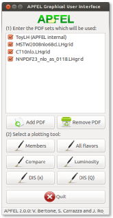
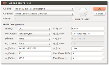
The APFEL GUI, starting from version 2.0.0, contains the following plotting tools:

• the “Members” tool: it plots all the members of a PDF set for a single parton flavor at a user-defined energy scale.

• The “All flavors” tool: each PDF flavor is plotted together in the same canvas. We also provide the possibility to scale PDF flavors by a predetermined factor.

• The “Compare” tool: it compares the same flavor of multiple PDF sets and the respective uncertainties.

• The “Luminosity” tool: it performs the computation of parton luminosities [75] normalized to a reference PDF set.

• The “DIS observables” tool: it computes the DIS observables as functions of $x$ or $Q$ for different heavy quark schemes.

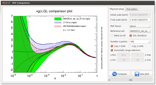
For all the various tools, there are several options for the graphical customization, like setting the axis ranges and axis titles. In Fig. 2 an example of the “Compare” tool is showed. APFEL also provides the possibility to save plots and the associated underlying data in multiple formats. All the results provided by the GUI for PDFs and parton luminosities from different PDF sets have been verified against the corresponding results from the PDF benchmarking exercise of Ref. [2].

Figure 2: Snapshot of the “Compare” tool available in the APFEL Graphical User Interface.

5 Validation and benchmarking

Having presented the methodology and the numerical techniques that APFEL adopts to solve the coupled QCD$\otimes$QED equations, and provided the relevant user documentation, we now turn to compare APFEL with other publicly available codes. First of all, we perform a detailed benchmarking of APFEL against HOPPET finding good agreement for the QCD evolution up to NNLO, both with pole and $\overline{\mathrm{MS}}$ heavy quark masses. Then we turn to the validation of the combined QCD$\otimes$QED evolution, and we compare the predictions of APFEL, using various options for the solution of the coupled evolution equations, with the partonevolution code, with the internal MRST04QED evolution and with the NNPDF internal code FastKernel.

In this section we also provide a study of the consistency of the different methods for the solution of the coupled QCD$\otimes$QED evolution equations, and show that when the QECD and QCED solutions are constructed iteratively in small steps in $Q^{2}$ so as to avoid introducing potentially large logarithms, they reduce numerically to the QavD solution. Finally, we provide results for the benchmarking of the DIS structure function module of APFEL.

5.1 QCD evolution

Figure 3: Comparison between PDFs evolved at NNLO in QCD using APFEL and HOPPET, from $Q_{0}^{2}=$2 GeV² up to $Q^{2}=$10⁴ GeV², using the Les Houches PDF benchmark settings. The comparison is performed in the pole mass scheme (left) and in the $\overline{\mathrm{MS}}$ scheme (right). The lower plots show the percent differences between the two codes.

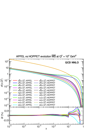
To begin with, we validate the QCD evolution in APFEL by comparing it with the results from the HOPPET program, version 1.1.5, up to NNLO, and using both pole and $\overline{\mathrm{MS}}$ heavy quark masses. The settings are the same as in the original Les Houches PDF evolution benchmark [71]. In the case of $\overline{\mathrm{MS}}$ masses, we take the $\overline{\mathrm{MS}}$ Renormalization-Group-Invariant charm mass $m_{c}(m_{c})$ to have the same numerical values as the pole masses. In all the comparisons in this section, the interpolation settings in APFEL are the default ones discussed in Sect. 3.

Results for the evolved PDFs at $Q^{2}=10^{4}$ GeV² for both HOPPET and APFEL are shown in Fig. 3. The left plot shows the results using pole masses, while the right plot corresponds to the case of $\overline{\mathrm{MS}}$ masses. Fig. 3 also shows the percent difference between both predictions, to show the excellent agreement obtained for the whole range in $x$, being at most $\sim 0.02\%$ at large-$x$, where PDFs have more structure.

5.2 QED evolution

We present now the numerical comparison of APFEL with three different QCD$\otimes$QED parton evolution codes: first partonevolution, then the internal evolution program used in the MRST04QED analysis, and finally the FastKernel program used in the NNPDF2.3QED analysis

5.2.1 Comparison with partonevolution

To begin with, we compare the results for the coupled QCD$\otimes$QED DGLAP evolution in APFEL with those of the public partonevolution code [49, 48], version 1.1.3.

Figure 4: Comparison between PDFs evolved at NLO in QCD (without QED corrections) with APFEL and partonevolution, from $Q_{0}^{2}=4$ GeV² up to $Q^{2}=10^{4}$ GeV². The same settings of the PDF benchmark study of Ref. [73] have been used. The lower plot shows the percent differences between the two codes.

Figure 5: Comparison between PDFs evolved at NLO in QCD and LO and QED using APFEL and partonevolution, from $Q_{0}^{2}=$4 GeV² up $Q_{0}^{2}=$10⁴ GeV² The same settings of the PDF benchmark study of Ref. [73] have been used. We show the comparison of quark and gluon PDFs using in APFEL the QCEDP solution (upper left plot), the QECDP solution (upper right plot), the QavDP solution (lower left plot) and then the photon PDF $\gamma(x,Q^{2})$ in the two codes for the different APFEL options. For each comparison, we also show the percent differences with respect to the partonevolution results.

To perform the benchmark, we use APFEL with the same settings used in the original publication [48] to present the numerical results of partonevolution, i.e. we take the input PDFs from the toy model used in the benchmarking exercise of Ref. [73], given by:

$$xu_{v}(x)=A_{u}x^{0.5}(1-x)^{3}\,,\quad xd_{v}(x)=A_{d}x^{0.5}(1-x)^{4}\,,$$

$$xS(x)=A_{S}x^{-0.2}(1-x)^{7}\,,\quad xg(x)=A_{g}x^{-0.2}(1-x)^{5}\,,$$

$$xc(x)=0\,,\quad x\bar{c}(x)=0\,,$$ (58)

at the initial scale $Q_{0}^{2}=4$ GeV², with a SU(3) symmetric sea that carries 15% of the proton’s momentum at $Q_{0}^{2}$, and only four active quarks are considered even above the bottom threshold. This toy model should not be confused with that used in the Les Houches PDF benchmark study, used elsewhere in this paper. In addition, the photon PDF is set to zero at the initial scale, that is $\gamma(x,Q_{0}^{2})=0$.

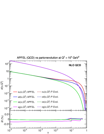
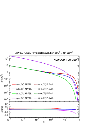
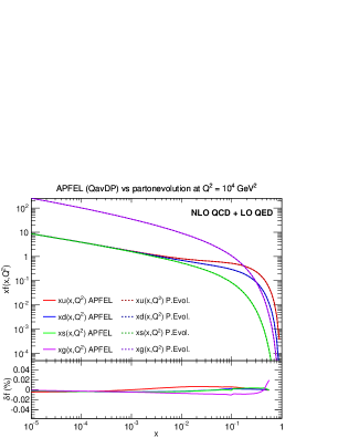
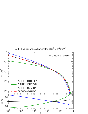
In order to set up the baseline, we ran the two codes at NLO QCD only, switching off the QED corrections. As can be seen from Fig. 4, good agreement is achieved. We can then move to the combined QCD$\otimes$QED evolution. Results are summarized in Fig. 5, where we compare the evolution of quark, gluon and photon PDFs given by the two codes, using the three different options for the solution of the coupled equations provided by APFEL: QCED, QECD and QavD (see Sect. 2). Note that in the fixed-flavor-number scheme the distinction between “series” and “parallel” solutions is immaterial. As expected, the best agreement between the two codes is obtained with the QavD option. As discussed in Sect. 2, this option ensures that the methods used for the solution of the evolution equations in the two codes differ only by $\mathcal{O}\left(\alpha^{2}\right)$ terms rather than by the larger $\mathcal{O}\left(\alpha\alpha_{s}\right)$ corrections. With these settings the evolution of quarks and gluon is essentially identical, with differences at most being $\mathcal{O}\left(0.01\%\right)$, while differences in the evolution of $\gamma(x,Q^{2})$ are below the few percent level except at the largest values of $x$.

The other two options, QCED and QECD, lead to differences in the PDF evolution of order $\mathcal{O}\left(\alpha\alpha_{s}\right)$ as compared to the partonevolution solution, corrections that, while being formally subleading, can be numerically large. For quark and gluon PDFs, the largest differences are seen for the gluon PDF, which can be up to 0.5% at the largest values of $x$. More substantial differences appear for the photon PDF, where of course higher-order QED effects are expected to be sizable. In the case of $\gamma(x,Q^{2})$, the three formally equivalent solutions can differ by up to 70%, both at small and large-$x$. As will be discussed below in Sect. 5.3, these large differences of the QCED and QECD solutions arise from unresummed large logarithms of the QCD and QED factorization scales. However, let us also recall that the order of magnitude is similar to that obtained in the comparison of LO and NLO evolution for the gluon PDF in QCD [77].

5.2.2 Comparison with MRST04QED

Another instructive comparison is provided by the QED evolution used in the determination of the MRST04QED parton distributions [32]. Though the original evolution code is not publicly available, the evolution which was used can be indirectly accessed via the public LHAPDF grids. In this case, it is not possible to use the Les Houches benchmark settings, and we are instead forced to use the same boundary conditions for the PDFs at $Q_{0}$ as those used in the MRST04QED fit as well as the same values of the heavy quark masses and reference coupling constants. The available MRST04QED fit was obtained at NLO in QCD in the VFN scheme, therefore it is possible to perform a meaningful comparison with the results of their evolution by using APFEL at NLO with the same settings.

Figure 6: Comparison between PDFs evolved using APFEL and the internal MRST04QED parton evolution, from $Q_{0}^{2}=$2 GeV² up to $Q^{2}=$10⁴ GeV². The boundary conditions for the PDFs are the same as those of the MRST04QED fit. PDF evolution is performed at NLO in QCD and LO in QED, in the variable-flavor number scheme. We show the comparison of quark and gluon PDFs using in APFEL the QCEDP solution (upper left plot), the QECDP solution (upper right plot), the QavDP solution (lower left plot) and then the photon PDF $\gamma(x,Q^{2})$ in the two codes for the different APFEL options.

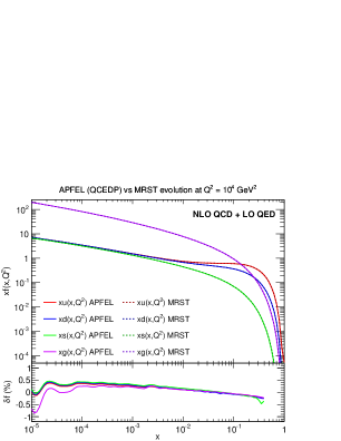
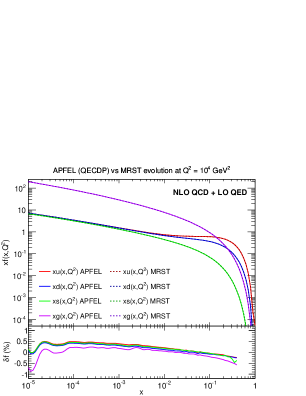
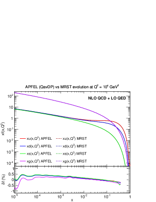
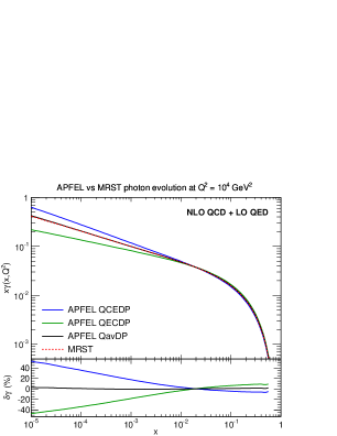
The comparison between the APFEL predictions and the MRST04QED evolution is shown in Fig. 6. PDFs have been evolved using APFEL and the internal MRST evolution from $Q_{0}^{2}=$2 GeV² up to $Q^{2}=$10⁴ GeV². We have explored the same three different options for the QCD$\otimes$QED combined evolution provided by APFEL as in the comparison with partonevolution, which differ only in the treatment of formally subleading terms. As can be seen from Fig. 6, for the evolution of the photon PDF the best agreement between APFEL and MRST04QED is achieved when the QavDP solution is used. The differences in this case are 1% at most for $\gamma(x,Q^{2})$ and much smaller for quark and gluon PDFs. It is also clear from Fig. 6 that other different options for solving the evolution equations in the presence of QED effects have a small impact on the evolution of quark and gluon PDFs, but for the photon PDF they can lead to differences up to 40% at small-$x$, for the reasons explained above. On the other hand, it should be taken into account that theoretical uncertainties in the QED evolution are subdominant with respect to the experimental uncertainties in the photon PDF at small-$x$ [33], due to the lack of experimental constraints.

5.2.3 Comparison with FastKernel

The third validation test of the QED evolution is provided by comparing the results of APFEL with the predictions given by the FastKernel internal NNPDF code [75]. This comparison is illustrative since the FastKernel code was used in the derivation of the NNPDF2.3QED sets, presented in Ref. [33] and where the FastKernel was compared to the partonevolution code finding reasonable agreement, with some small differences arising from a different treatment of the subleading terms. Now we revisit this issue using the APFEL flexibility to explore different options for the solution of the QCD$\otimes$QED coupled evolution equations.

Figure 7: The evolution of the photon PDF $\gamma(x,Q^{2})$ at NLO in QCD and LO in QED for various values of $Q^{2}$, performed both with APFEL and with FastKernel. The Les Houches benchmark settings have been used, supplemented by the boundary condition $x\gamma(x,Q^{2}_{0})=0$, with $Q^{2}_{0}=2$ GeV². For APFEL, the QECDS solution has been used. The lower plot shows the percent difference between the two calculations.

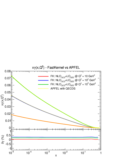
The basic strategy underlying the FastKernel code [51] is to solve the evolution equations in Mellin space and then invert the evolution kernels back to $x$ space, where they are convoluted with the initial $x$-space PDFs to obtain the evolved PDFs. The NNPDF2.3QED sets use the truncated solution for the Mellin space DGLAP equations, and so cannot directly be compared with APFEL, which is based instead on the expanded solution (as any $x$-space code). Therefore, for the purpose of this benchark comparison, we have produced the combined NLO QCD and LO QED predictions with the FastKernel code using the expanded solution of the Mellin space equations, and compared them to the APFEL results.

The comparison is presented in Fig. 7. We show the evolution of the photon PDF $\gamma(x,Q^{2})$ at NLO in QCD and LO in QED for various values of $Q^{2}$, performed both with APFEL and with the FastKernel code. For APFEL, the QECDS solution has been used: this is indeed equivalent to the procedure that has been used in the NNPDF2.3QED fits. The Les Houches benchmark settings have been adopted, supplemented by the boundary condition $\gamma(x,Q^{2}_{0})=0$, with $Q^{2}_{0}=$2 GeV². In the lower plot of Fig. 7 we provide the percent differences between the two calculations. As can be seen, differences are small, at the few per-mil level, showing that the two codes are in good agreement when common settings are adopted.

In summary, the QCD$\otimes$QED evolution used in the NNPDF2.3QED fits differs from that used in other codes, such as partonevolution and MRST04QED, only by higher-order terms: truncated versus iterated solution of the evolution equations in Mellin space and different treatment of the subleading $\mathcal{O}\left(\alpha\alpha_{s}\right)$ terms. As has been shown in Figs. 5 and 6, while for quark and gluon PDFs these differences are small, for the photon PDF these inherent theoretical uncertainties are substantial and could possibly be reduced including higher-order corrections in the QED coupling in the combined evolution equations. Such improvements might be required by future, more precise experimental data.

5.3 Consistency of the coupled solution

Now we turn to discuss the consistency of the procedure adopted in APFEL to combine the solutions of the QCD and QED evolution equations. As presented in Sect. 2, the combination of QCD and QED solutions in APFEL is perfomed at the level of the evolution operators, rather than at the level of splitting functions, as done, for instance, in the partonevolution and MRST04QED codes. This procedure leads to the introduction of two different factorization scales, $\mu_{\rm QCD}$ and $\mu_{\rm QED}$, which in principle are allowed to vary in a fully independent way.

A possible objection to this approach is that, in the case in which $\mu_{\rm QCD}$ and $\mu_{\rm QED}$ are very different from each other, this procedure might lead to the presence of numerically large, unresummed logarithms. On the other hand, in Sect. 2 we showed that these terms are $\mathcal{O}\left(\alpha\alpha_{s}\right)$ for the QECD and the QCED solutions and $\mathcal{O}\left(\alpha^{2}\right)$ for the QavD solution, that are both perturbatively subleading.

In order quantify the impact of these potentially large (subleading) logarithms, we have performed with APFEL the combination of QCD and QED evolutions not over the whole (possibly large) $\left[Q_{0},Q\right]$ range, but rather dividing it in small intervals $\left[Q_{0},Q_{1}\right]$, $\left[Q_{1},Q_{2}\right]$, $\ldots$, $\left[Q_{N},Q\right]$, and performing the combination on each interval. This procedure ensures that no artificially large logarithm of two widely different scales appears in the solution. An example of how to construct this small-step approximation with the available functions of APFEL has been included in the example folder of the main source folder.

As an illustration, using again the settings of the Les Houches PDF evolution benchmark [71], supplemented by the ansatz $\gamma(x,Q_{0})=0$, we have evolved the PDFs between $Q_{0}^{2}=2$ GeV² and $Q^{2}=10000$ GeV². We have then compared the standard, single-step solution with the new solution sketched above and based on combining the results of many small evolution steps. As expected, no significant differences were observed for quarks and gluon, so in the following we concentrate on the different results for the evolution of the photon PDF.

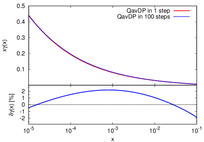
In Fig. 8 we compare the standard QavD solution, performed with a single step between $Q_{0}^{2}$ and $Q^{2}$, with the corresponding solution where the full range $\left[Q_{0}^{2},Q^{2}\right]$ has been divided into 100 logarithmically spaced intervals. In the bottom panel of Fig. 8 we show the percentage difference between the two results: reasonable agreement is found, with small residual differences at the level of 2% at most. This comparison confirms that the QavDP solution adopted in APFEL is free of numerically large scale logarithms and that a single $Q^{2}$ interval leads to reliable results. The small impact of potentially large logarithms can be explained considering that they are suppressed by a factor $\alpha^{2}$.

Figure 8: Evolution of the photon PDF $\gamma(x,Q^{2})$ between $Q_{0}^{2}=2$ GeV² and 10⁴ GeV² with the QavDP solution. We compare the evolution performed with a single step with that obtained with 100 steps logarithmically spaced in $Q^{2}$. The lower panel shows the percentage differences between the two methods.

Once we have explicitly verified that no large unresummed logarithms are present in the QavD solution, we turn to consider the QECD and the QCED solutions. The results for the 100-step evolution of the photon PDFs in these two cases are shown in Fig. 9 and compared to the one-step QavD solution. We see that, unlike the case where a single step is used (see Fig. 6) and where differences up to 40% were observed (though only for small values of $x$), now differences between the three solutions are 2% at most. This suggests that the $\mathcal{O}\left(\alpha\alpha_{s}\right)$ logarithmic terms that affect the QECD and the QCED solutions are numerically large and may spoil the respective perturbative evolution unreliable if the evolution interval is too wide.

Figure 9: Comparison of the evolution of the photon PDF $\gamma(x,Q^{2})$ between $Q_{0}^{2}=2$ GeV² and 10⁴ GeV² obtained with the QavDP solution with a single step, with those of the QECDP and QCEDP solutions with 100 logarithmically spaced steps. The lower panel shows the percentage differences between the two methods.

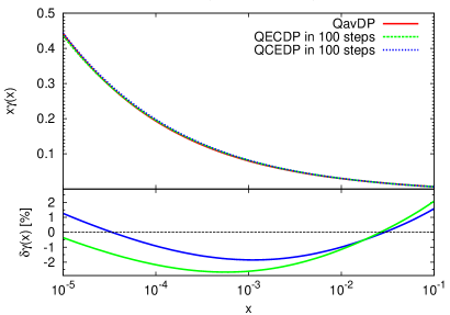
Therefore, we can conclude that the QavD solution of the coupled QCD$\otimes$QED evolution equations is the most reliable one, since in this case potentially large unresummed scale logarithms are absent. On the other hand, this analysis also shows that the QECD and the QCED solutions may introduce artificially large logarithms and that an effective way to cancel them is to perform the evolution in small steps combining sequentially the results. In this case, the results from the QECD and the QCED solutions coincide to a good approximation with that of the QavD solution, so that all three strategies lead to the same numerical solution.

5.4 Deep-Inelastic Scattering structure functions

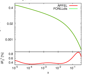
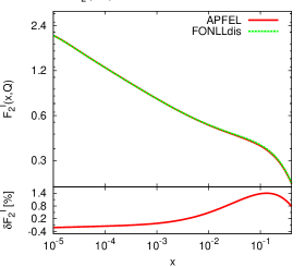
Finally, in this section we briefly document the benchmarking of the DIS module implemented in APFEL against the publicly available code FONLLdis [52], which computes the charm structure functions in the FONLL GM-VFN scheme using the exact $x$-space $\mathcal{O}\left(\alpha_{s}^{2}\right)$ heavy quark coefficient functions. The FONLLdis code provides predictions for the electromagnetic structure functions $F_{2}^{l}$, $F_{2}^{c}$, $F_{L}^{l}$ and $F_{L}^{c}$ up to $\mathcal{O}\left(\alpha_{s}^{2}\right)$ in the FONLL scheme. In Fig. 10 we compare the predictions for $F_{2}^{l}$ (left plot) and $F_{2}^{c}$ (right plot) at $Q^{2}=10$ GeV² obtained with APFEL with those obtained with FONLLdis using the Les Houches heavy quark Benchmark settings [78]. As can be seen from the bottom panel of Fig. 10, the relative differences between APFEL and FONLLdis are always well below the percent level for $F_{2}^{c}$ and at most of 1.3% for $F_{2}^{l}$: a more than reasonable accuracy for phenomenology.

Figure 10: Comparison between APFEL and FONLLdis [52] for the charm structure function $F_{2}^{c}$ (left) and the light structure function $F_{2}^{l}$ (right) in the FONLL-C scheme in the range $x\in[10^{-5}:10^{-1}]$ at $Q^{2}=10$ GeV². The lower panel displays the percentage different in percent between the two computations.

6 Conclusions and outlook

APFEL is a new PDF evolution library that combines NNLO QCD corrections with LO QED effects in the solution of the DGLAP equations. It is the first public evolution code that allows to perform the coupled QCD$\otimes$QED evolution up to NNLO in $\alpha_{s}$ and LO in $\alpha$, both in the FFN and VFN schemes, and using either pole or $\overline{\mathrm{MS}}$ heavy quark masses. It is fast, accurate, and flexible, and can be easily accessed through its Fortran 77, C/C++ and Python interfaces. From version 2.0.0, the APFEL capabilities have been extended to include a new module that computes neutral- and charged-current DIS observables up to $\mathcal{O}(\alpha_{s}^{2})$ in the FONLL scheme [52]. In addition, we provide a flexible user-friendly Graphical User Interface which provides access to all of the APFEL functionalities without the need of writing code and to produce high-quality plots in various different formats.

Given the relevance of QED and electroweak corrections for precision theoretical predictions at the LHC in the coming years, and the corresponding needs for parton distributions that consistently include QED effects, we believe that a library like APFEL can become a useful tool for the PDF fitting community.

In the short term, we plan to extend the capabilities of APFEL to include the solution of DGLAP equations with (N)NLO time-like splitting functions [79], such as those required in global fits of fragmentation functions [80], as well as the evolution for polarized PDFs up to NLO, which could be of interest in the determinations of spin-dependent parton distributions [81, 82, 83]. Another feature foreseen in future releases is the implementation of different factorization schemes for the PDF evolution, such as the DIS or the AB scheme, the latter useful in the context of polarized fits [84]. In addition, while the current release of APFEL allows only the evolution of the proton PDFs, future releases will also allow to simultaneously evolve both proton and neutron PDFs. This feature is important to enable dedicated studies of isospin symmetry violation, both at low scales (non-perturbative) and at high scales, with an additional component generated dynamically by the presence of QED effects in the evolution [33, 32].

In a longer timescale, an appealing possibility consists of the inclusion of high-energy (small-$x$) resummation effects in the splitting functions [85, 86] and their matching with the fixed order expressions, a feature which is not present in any public evolution code yet. Another possible interesting extension, where more theory work is also required, would be the implementation of the pure electroweak corrections to PDF evolution [87, 88]. In order to improve the perturbative accuracy of the QED evolution in the DGLAP evolution, one could attempt to achieve higher-order accuracy in $\alpha$. This would imply the inclusion of the mixed splitting functions, proportional to $\mathcal{O}\left(\alpha\alpha_{s}\right)$, as well as of the $\mathcal{O}\left(\alpha^{2}\right)$ corrections, requiring however substantial modifications in the structure of APFEL. Including higher-order corrections in the QED expansion might eventually be required when future, more accurate LHC data in processes like low- and high-mass Drell-Yan production and high invariant mass $WW$ production become available. Another possibility worth exploring in this sense is the use of precise data on photo-production at HERA [89] to obtain additional information of the photon PDF.

The APFEL program is available from its HepForge website:

http://apfel.hepforge.org/ 

and it can also be accessed directly from the svn repository, both the development trunk:

svn checkout http://apfel.hepforge.org/svn/trunk apfel

as well as the current stable release:

svn checkout http://apfel.hepforge.org/svn/tags/2.0.0 apfel-2.0.0

Acknowledgments
We are grateful to Stefano Forte for discussions about QED corrections in PDFs, to Gavin Salam for his comments on the manuscript and to Stefan Weinzierl for providing useful information about the partonevolution1.1.3 package. We also thank Emanuele Nocera for testing the GUI and providing useful feedback. We finally thank the referee for insightful comments about the differences between the various options for solving the coupled QCD$\otimes$QED evolution equations in APFEL. V. B. is supported by the ERC grant 291377, ”LHCtheory: Theoretical predictions and analyses of LHC physics: advancing the precision frontier”. S. C. is supported by an Italian PRIN 2010 and by a European EIBURS grant. J. R. is partially supported by a Marie Curie Intra–European Fellowship of the European Community’s 7th Framework Programme under contract number PIEF-GA-2010-272515.

References

- [1] S. Forte and G. Watt, (2013), 1301.6754.
- [2] R.D. Ball et al., JHEP 1304 (2013) 125, 1211.5142.
- [3] A. De Roeck and R. Thorne, Prog.Part.Nucl.Phys. 66 (2011) 727, 1103.0555.
- [4] U. Baur, S. Keller and D. Wackeroth, Phys.Rev. D59 (1999) 013002, hep-ph/9807417.
- [5] V. Zykunov, Eur.Phys.J.direct C3 (2001) 9, hep-ph/0107059.
- [6] S. Dittmaier and M. Kramer, Phys.Rev. D65 (2002) 073007, hep-ph/0109062.
- [7] U. Baur et al., Phys.Rev. D65 (2002) 033007, hep-ph/0108274.
- [8] U. Baur and D. Wackeroth, Phys.Rev. D70 (2004) 073015, hep-ph/0405191.
- [9] A. Arbuzov et al., Eur.Phys.J. C54 (2008) 451, 0711.0625.
- [10] A. Arbuzov et al., Eur.Phys.J. C46 (2006) 407, hep-ph/0506110.
- [11] S. Brensing et al., Phys.Rev. D77 (2008) 073006, 0710.3309.
- [12] G. Balossini et al., JHEP 1001 (2010) 013, 0907.0276.
- [13] C. Carloni Calame et al., JHEP 0710 (2007) 109, 0710.1722.
- [14] S. Dittmaier and M. Huber, JHEP 1001 (2010) 060, 0911.2329.
- [15] A. Denner et al., JHEP 0908 (2009) 075, 0906.1656.
- [16] A. Denner et al., JHEP 1106 (2011) 069, 1103.0914.
- [17] A. Denner et al., Eur.Phys.J. C73 (2013) 2297, 1211.5078.
- [18] J. Baglio, L.D. Ninh and M.M. Weber, (2013), 1307.4331.
- [19] A. Bierweiler et al., JHEP 1211 (2012) 093, 1208.3147.
- [20] M. Luszczak and A. Szczurek, (2013), 1309.7201.
- [21] S. Moretti, M. Nolten and D. Ross, Phys.Rev. D74 (2006) 097301, hep-ph/0503152.
- [22] S. Dittmaier, A. Huss and C. Speckner, JHEP 1211 (2012) 095, 1210.0438.
- [23] W. Bernreuther, M. Fuecker and Z. Si, Phys.Lett. B633 (2006) 54, hep-ph/0508091.
- [24] J.H. Kühn, A. Scharf and P. Uwer, Eur.Phys.J. C45 (2006) 139, hep-ph/0508092.
- [25] W. Hollik and M. Kollar, Phys.Rev. D77 (2008) 014008, 0708.1697.
- [26] W. Hollik and D. Pagani, Phys.Rev. D84 (2011) 093003, 1107.2606.
- [27] J. Kühn, A. Scharf and P. Uwer, (2013), 1305.5773.
- [28] K. Mishra et al., (2013), 1308.1430.
- [29] A. De Rujula, R. Petronzio and A. Savoy-Navarro, Nucl.Phys. B154 (1979) 394.
- [30] J. Kripfganz and H. Perlt, Z.Phys. C41 (1988) 319.
- [31] J. Blumlein, Z.Phys. C47 (1990) 89.
- [32] A.D. Martin et al., Eur. Phys. J. C39 (2005) 155, hep-ph/0411040.
- [33] The NNPDF Collaboration, R.D. Ball et al., (2013), 1308.0598.
- [34] S. Carrazza, (2013), 1307.1131.
- [35] S. Carrazza, (2013), 1305.4179.
- [36] D. Bourilkov, R.C. Group and M.R. Whalley, (2006), hep-ph/0605240.
- [37] T. Sjostrand, S. Mrenna and P.Z. Skands, Comput. Phys. Commun. 178 (2008) 852, 0710.3820.
- [38] S. Carrazza, S. Forte and J. Rojo, (2013), 1311.5887.
- [39] G.P. Salam and J. Rojo, Comput. Phys. Commun. 180 (2009) 120, 0804.3755.
- [40] A. Cafarella, C. Coriano and M. Guzzi, Comput.Phys.Commun. 179 (2008) 665, 0803.0462.
- [41] M. Botje, Comput.Phys.Commun. 182 (2011) 490, 1005.1481.
- [42] P.G. Ratcliffe, Phys.Rev. D63 (2001) 116004, hep-ph/0012376.
- [43] L. Schoeffel, Nucl.Instrum.Meth. A423 (1999) 439.
- [44] C. Pascaud and F. Zomer, (2001), hep-ph/0104013.
- [45] A. Vogt, Comput. Phys. Commun. 170 (2005) 65, hep-ph/0408244.
- [46] D.A. Kosower, Nucl.Phys. B506 (1997) 439, hep-ph/9706213.
- [47] H. Spiesberger, Phys.Rev. D52 (1995) 4936, hep-ph/9412286.
- [48] M. Roth and S. Weinzierl, Phys.Lett. B590 (2004) 190, hep-ph/0403200.
- [49] S. Weinzierl, Comput.Phys.Commun. 148 (2002) 314, hep-ph/0203112.
- [50] The NNPDF collaboration, L. Del Debbio et al., JHEP 03 (2007) 039, hep-ph/0701127.
- [51] The NNPDF Collaboration, R.D. Ball et al., Nucl. Phys. B809 (2009) 1, 0808.1231.
- [52] S. Forte et al., Nucl. Phys. B834 (2010) 116, 1001.2312.
- [53] The NNPDF Collaboration, R.D. Ball et al., Phys.Lett. B723 (2013) 330, 1303.1189.
- [54] G. Altarelli and G. Parisi, Nucl. Phys. B126 (1977) 298.
- [55] V.N. Gribov and L.N. Lipatov, Sov. J. Nucl. Phys. 15 (1972) 438.
- [56] Y.L. Dokshitzer, Sov. Phys. JETP 46 (1977) 641.
- [57] E. Floratos, D. Ross and C. Sachrajda, Nucl.Phys. B129 (1977) 66.
- [58] E. Floratos, D. Ross and C. Sachrajda, Nucl.Phys. B152 (1979) 493.
- [59] A. Gonzalez-Arroyo, C. Lopez and F. Yndurain, Nucl.Phys. B153 (1979) 161.
- [60] E. Floratos, C. Kounnas and R. Lacaze, Nucl.Phys. B192 (1981) 417.
- [61] G. Curci, W. Furmanski and R. Petronzio, Nucl.Phys. B175 (1980) 27.
- [62] S. Moch, J. Vermaseren and A. Vogt, Nucl.Phys. B688 (2004) 101.
- [63] S. Moch, J. Vermaseren and A. Vogt, Phys. Lett. B691 (2004) 129.
- [64] M. Buza et al., Nucl. Phys. B472 (1996) 611, hep-ph/9601302.
- [65] H1 Collaboration, F. Aaron et al., JHEP 1209 (2012) 061, 1206.7007.
- [66] R.D. Ball et al., Nucl. Phys. B849 (2011) 296, 1101.1300.
- [67] M. Aivazis et al., Phys.Rev. D50 (1994) 3102, hep-ph/9312319.
- [68] M. Guzzi et al., Phys.Rev. D86 (2012) 053005, 1108.5112.
- [69] R. Thorne, Phys.Rev. D86 (2012) 074017, 1201.6180.
- [70] W. Giele et al., (2002), hep-ph/0204316.
- [71] M. Dittmar et al., (2005), hep-ph/0511119.
- [72] W. Giele et al., (2002) 275, hep-ph/0204316.
- [73] J. Blumlein et al., (1996), hep-ph/9609400.
- [74] NuTeV, M. Goncharov et al., Phys. Rev. D64 (2001) 112006, hep-ex/0102049.
- [75] The NNPDF collaboration, R.D. Ball et al., Nucl. Phys. B838 (2010) 136, 1002.4407.
- [76] V. Bertone and J. Rojo, AIP Conf.Proc. 1523 (2012) 51, 1212.0741.
- [77] NNPDF Collaboration, R.D. Ball et al., Nucl.Phys. B855 (2012) 153, 1107.2652.
- [78] SM and NLO Multileg Working Group, J. Andersen et al., (2010) 21, 1003.1241.
- [79] A. Mitov, S. Moch and A. Vogt, Phys.Lett. B638 (2006) 61, hep-ph/0604053.
- [80] D. de Florian, R. Sassot and M. Stratmann, Phys.Rev. D76 (2007) 074033, 0707.1506.
- [81] The NNPDF Collaboration, R.D. Ball et al., Nucl.Phys. B874 (2013) 36, 1303.7236.
- [82] D. de Florian et al., Phys. Rev. D80 (2009) 034030, 0904.3821.
- [83] E. Leader, A.V. Sidorov and D.B. Stamenov, Phys.Rev. D82 (2010) 114018, 1010.0574.
- [84] G. Altarelli et al., Acta Phys.Polon. B29 (1998) 1145, hep-ph/9803237.
- [85] G. Altarelli, R.D. Ball and S. Forte, Nucl. Phys. B799 (2008) 199, 0802.0032.
- [86] M. Ciafaloni et al., JHEP 0708 (2007) 046, 0707.1453.
- [87] M. Ciafaloni, P. Ciafaloni and D. Comelli, Phys.Rev.Lett. 88 (2002) 102001, hep-ph/0111109.
- [88] P. Ciafaloni and D. Comelli, JHEP 0511 (2005) 022, hep-ph/0505047.
- [89] M. Klasen, Rev.Mod.Phys. 74 (2002) 1221, hep-ph/0206169.