Nonequilibrium Statistical Mechanics of Systems with Long-Range Interactions: Ubiquity of Core-Halo Distributions
Abstract
Systems with long-range (LR) forces, for which the interaction potential decays with the interparticle distance with an exponent smaller than the dimensionality of the embedding space, remain an outstanding challenge to statistical physics. The internal energy of such systems lacks extensivity and additivity. Although the extensivity can be restored by scaling the interaction potential with the number of particles, the non-additivity still remains. Lack of additivity leads to inequivalence of statistical ensembles. Before relaxing to thermodynamic equilibrium, isolated systems with LR forces become trapped in out-of-equilibrium quasi-stationary state (qSS), the lifetime of which diverges with the number of particles. Therefore, in thermodynamic limit LR systems will not relax to equilibrium. The qSSs are attained through the process of collisionless relaxation. Density oscillations lead to particle-wave interactions and excitation of parametric resonances. The resonant particles escape from the main cluster to form a tenuous halo. Simultaneously, this cools down the core of the distribution and dampens out the oscillations. When all the oscillations die out the ergodicity is broken and a qSS is born. In this report, we will review a theory which allows us to quantitatively predict the particle distribution in the qSS. The theory is applied to various LR interacting systems, ranging from plasmas to self-gravitating clusters and kinetic spin models.
keywords:
long-range interactions , Vlasov equation , collisionless relaxation , quasi-stationary states , nonequilibrium statistical mechanics1 Introduction
A long time ago Einstein expressed his belief that thermodynamics is “the only physical theory of universal content concerning which I am convinced that, within the framework of applicability of its basic concepts, it will never be overthrown” [1]. One can, however, wonder about the extent of the “applicability” to which Einstein was referring. For example, can thermodynamics in any form be applied to study non-neutral plasmas or galaxies in which “particles” interact by long-range (LR) forces?
The difficulty of studying systems with LR interactions was already well appreciated by Gibbs, who noted the inapplicability of statistical mechanics when interparticle potentials decay with exponents smaller than the dimensionality of the embedding space [2, 3]. For such systems energy is not extensive and traditional thermodynamics fails. One way to correct the lack of extensivity is to scale the interaction energy with the inverse of the number of particles. This is the so-called Kac prescription designed to restore extensivity to the free energy [4, 5, 6]. The problem, however, remains — although the energy is now extensive, it is still non-additive. On the other hand, it is a fundamental postulate of thermodynamics that entropy and energy must be additive over the subsystems — that is, the interfacial contributions should be negligibly small. For systems with short-range forces this condition is clearly satisfied — in the thermodynamic limit the interfacial energy is much smaller than the energy of the bulk. This, however, is not true for systems with LR forces for which the interfacial region cannot be clearly defined [7] — every particle interacts with every other particle of the system, so that no clear separation into bulk and interface exists.
One can still hope that although the additivity of energy breaks down, it might still be possible to use equilibrium statistical mechanics to describe stationary states of systems with LR interactions. Very quickly, however, one runs into difficulties. For example, depending on the ensemble used, one finds that a system can remain either in one phase or undergo a phase transition [8]. One also finds that in the microcanonical ensemble such systems can have negative specific heat [9, 10, 11, 12, 13, 14], contrary to the laws of usual thermodynamics.
There is, however, an even more profound problem with applying classical statistical mechanics to systems with LR forces. The underlying assumption of Boltzmann-Gibbs (BG) statistics is the existence of ergodicity and mixing [15]. For a closed system of particles (in a microcanonical ensemble) the initial distribution should uniformly spread over the available phase space, so that in equilibrium all microstates corresponding to a given thermodynamic macrostate should be equally probable. Although there is no general proof of ergodicity and mixing, in practice it has been found to apply to most nonintegrable systems with short-range forces. There is, however, no indication that ergodicity and mixing exist for systems with LR interactions [16, 17, 18, 7, 19]. In fact, one should expect precisely the opposite. Kac renormalization of the interaction potential kills off the correlations between particles. Within the kinetic theory, it is precisely these correlations (collisions) that drive a system to thermodynamic equilibrium. In the absence of correlations, the dynamical evolution of the one-particle distribution function is governed by the collisionless Boltzmann (Vlasov) equation [20, 21]. Starting from an arbitrary initial condition, a solution of this equation does not evolve to a stationary state — the spatiotemporal evolution continues ad infinitum on smaller and smaller length scales. It is only in a coarse-grained sense that we can say that the system has reached an “equilibrium” — a finite resolution imposed on us by an experiment or a computer simulation will not allow us to see the full fine-grained evolution of the distribution function. The coarse-grained stationary state will, in general, be very different from the normal thermodynamic equilibrium. Unlike the state of thermodynamic equilibrium, it will explicitly depend on the initial distribution of particle positions and velocities [22]. In particular, the velocity distribution in the stationary state (SS) will not have the characteristic Maxwell-Boltzmann form [23, 24, 25]. Indeed, observations and simulations of both gravitational clusters [26, 27, 28, 29, 30, 31, 32, 33, 34, 35, 36, 37, 38, 39, 40] and confined non-neutral plasmas [41, 42, 43, 44, 45, 46, 47, 48, 49, 50, 51, 52, 23], indicate presence of such nonequilibrium stationary states.
It is, therefore, clear that in the thermodynamic limit, traditional methods of equilibrium statistical mechanics cannot be applied to systems with LR forces. A new theory is needed. The goal of the present Report is to show how such theory can be constructed. Using the properties of Vlasov dynamics and the theory of parametric resonances, we will derive coarse-grained distribution functions for the nonequilibrium stationary states of systems with LR interactions, without explicitly solving the collisionless Boltzmann equation. Comparing the theory with the explicit -body simulations, we will show that it is able to quantitatively predict both position and velocity distribution functions of self-gravitating clusters [38, 39, 53], magnetically confined plasmas [23, 24], and of kinetic spin models [54, 55, 25], without any adjustable parameters. We will focus on statistical theory of nonequilibrium quasi-stationary states; only briefly shall we address the thermodynamic equilibrium, which has already been thoroughly covered by Campa et al in Ref [7].
The Report is organized as follows: in section 1 we begin with an introduction to the principal properties of systems with LR interactions, followed by a review of the Vlasov dynamics. Sections 2, 3, and 4 present results for self-gravitating clusters in one, two, and three dimensions, respectively. In section 5 we address the non-equilibrium properties of magnetically confined plasmas, and in sections 6 and 7 we discuss two different kinetic spin models. Section 8 concludes the Report, reviewing the theories and the results obtained so far and outlining the perspectives for future research.
2 Systems with Long Range Forces
Among the physical systems, a significant fraction involves those whose particles interact by long-range potentials of the form , where and is the dimensionality of the embedding space. Examples of such systems include galaxies and globular clusters [56, 57, 58, 59, 60, 61, 62, 63, 64], two-dimensional and geophysical flows and vortex models [18, 65, 66, 67, 68, 69, 70], quantum spin models [71], dipolar excitons [72], cold atom models [73], as well as magnetically confined plasmas [74, 75, 76, 23]. In order to predict the behavior of systems with short-range forces we can rely on thermodynamics and statistical mechanics both of which, however, fail for systems with LR interactions.
Thermodynamics requires extensivity and additivity [77], neither of which is valid for LR systems [7]. A system of particles confined inside a volume is said to be extensive if, when the number of particles and the volume are scaled by , the internal energy of the system scales as . It is easy to see that systems with short-range forces are extensive. If the interaction potential is short-range, each particle will interact only with the particles which are within the range of the interaction potential. Suppose that a system is homogeneous, the number of particles within the distance of a given particle will then be proportional to and the internal energy must have the form of , where is a function that depends on the microscopic interactions between the particles. This form of internal energy is clearly extensive. In fact, it is not necessary for the interaction potential to be strictly short-range — bounded by — algebraically decaying potentials will lead to extensive thermodynamics as long as they decay sufficiently rapidly, i.e. if [78]. We shall call all such systems “finite range”.
Extensivity is important for the existence of a nontrivial thermodynamic limit and the equivalence of different statistical ensembles. A thermodynamic system in contact with a thermal reservoir at temperature — canonical ensemble — must be at the minimum of its Helmholtz free energy , where is the entropy. The celebrated Boltzmann formula relates the thermodynamics with dynamics by associating , the number of microstates available to the system through its dynamics, to the concept of entropy of classical thermodynamics. The phase space volume of a confined Hamiltonian system, which is proportional to , grows exponentially with the number of particles so that , irrespective of the range of interactions. Therefore, both the internal energy and entropy of a finite range system scale linearly with the number of particles in the system, allowing for a nontrivial thermodynamic equilibrium.
LR systems, however, are intrinsically different. The infinite range of the interaction potential results in an internal energy that scales superlinearly with the number of particles in the system, . Therefore if such system is put in contact with a thermal bath, for large the Helmholtz free energy will be dominated by the internal energy. The equilibrium state will then correspond to the minimum of the internal energy . The entropy will be irrelevant, unless the temperature of the reservoir is unrealistically large and scales with the number of particles in the system, .
In practice, most LR systems are isolated from the environment. This is the case for galaxies and magnetically confined plasmas. Gravity in three dimensions is particularly challenging because of the evaporation of particles [26, 79, 80]; however, one and two dimensional gravitational systems and magnetically confined plasmas can be studied straightforwardly using molecular dynamics simulations (MD). Unlike systems with short-range forces — which must be confined to a box in order to have a nontrivial thermodynamics — one and two dimensional gravitational systems are self-confining and can exist in an infinite volume, . Once again, however, one runs into a difficulty with the long-range nature of the interaction potential. The superextensive interaction energy leads to strong forces and velocities which rapidly exceed that of the speed of light. To avoid this problem and to obtain a well defined thermodynamic limit it is necessary to rescale the gravitational coupling constant by a factor . This is the so-called Kac prescription [4]. For a gravitational system of particles in an infinite volume, the Kac prescription is equivalent to the requirement that the mass of each particle , while remains finite, . One can show that this leads to a well defined thermodynamic limit as .
Although the rescaled gravity and plasmas are extensive, they remain nonadditive. For a -dimensional system of particles interacting by a finite-range potential, the interfacial energy scales with the number of particles as , while the bulk energy grows as . Thus, the total energy of a finite-range system in the thermodynamic limit is equivalent to the sum of the energies of its macroscopic subsystems. This is not true for LR systems. As the interaction range grows, the concept of interface loses its meaning. One can no longer consider a total system as a sum of smaller subsystems, since the LR nature of the potential leads to a nontrivial interaction between all the subsystems. The lack of additivity can result in a negative specific heat for an isolated LR system [9, 10, 12, 7]. On the other hand, if a LR system is in contact with a thermal bath, its specific heat must be positive. Contrary to what happens with finite-range systems the predictions of microcanonical and canonical ensembles may, therefore, be inequivalent for systems with LR interactions [81, 82, 83, 84]. Similarly, the canonical and the grand-canonical ensembles may also become inequivalent [85]. Besides inequivalence of ensembles, it has also been debated that negative specific heat may result in yet another abnormality: the violation of the zeroth law of thermodynamics [86, 87, 88, 89].
Another difficulty with the statistical treatment of LR systems is the lack of ergodicity. The ergodic theorem allows us to replace the time averages by the ensemble averages [90]. Consider a dimensional phase space of interacting particles. Each point in this phase space represents a possible configuration (microstate) of the system. For a given thermodynamic macrostate there is a huge number of possible microstates. This allows us to define a statistical ensemble of microstates with a probability density . The dynamics of is governed by the Liouville equation. For equilibrium statistical mechanics to work, the initial probability density should uniformly spread over the energy surface — producing a, so-called, mixing flow [15].
The fundamental problem of ergodic theory is to understand under what conditions a nonstationary phase space density will converge to a stationary one [91, 92]. Note that for a time reversible system one can not have a “fine-grained” equilibrium, a thermodynamic equilibrium exists only in a coarse-grained sense. On a fine-grained scale, the dynamical evolution of the probability density will never stop, so that if at some point during the dynamical evolution the velocities of all the particles are reversed, the system will diverge from the equilibrium. Although ergodicity and mixing have been verified for many different systems with finite-range forces, both seem to fail for systems with LR interactions [16, 17, 93, 19].
The relaxation to a stationary state (SS) of systems with LR interactions is fundamentally different from the relaxation to equilibrium of systems with short-range forces. For the latter, the relaxation is collisional and the reduced probability densities are governed by the BBGKY (Born, Bogoliubov, Green, Kirkwood, Yvon) hierarchy of equations [94]. At the leading order of this hierarchy is the Boltzmann equation , where is the convective derivative of and . This equation describes the evolution of the one-particle distribution function [95]. The right hand side of the Boltzmann equation is the collision term that drives the system towards thermodynamic equilibrium [95]. The distribution functions in thermodynamic equilibrium do not depend on the initial condition, but only on the global conserved quantities, and are described by the Boltzmann-Gibbs statistical mechanics [96].
The situation is very different for systems with LR forces. In the thermodynamic limit the dynamics of these systems is completely dominated by the mean-field and the collisions (correlations) are negligible. To see why this is so, let us consider, for example, a one dimensional gravitational system of particles of mass , interacting by , where is the gravitational constant. As was discussed above, to have a well defined thermodynamic limit we need to require that , while the total mass of the system remains fixed, . Although the interaction between any two particles is vanishingly small, the infinite range of the potential results in a finite total force acting on each particle. To quantify the discreteness (correlations) effects [97] we can define a plasma parameter — corresponding to the ratio of the characteristic two-body interaction energy and the average kinetic energy — , where is the average particle velocity and is a characteristic separation between the particles. measures the degree to which the dynamics of a system is dominated by the correlations — if the correlations (collisions) are important and if the dynamics is governed purely by the mean-field. Starting from an initial particle distribution, a one dimensional gravitational cluster will relax to a stationary state, with a characteristic velocity . It will be shown in the following sections that the extent of the mass distribution is controlled by the parametric resonances, so that starting from an initial particle distribution with a compact support, the final distribution will be restricted to a finite "volume" or radius , so that . We then come to the conclusion that , in the thermodynamic limit the correlations vanish and the dynamics of a LR system is determined purely by the mean-field.
The argument above suggests that for LR systems the (collisional) right-hand side of the Boltzmann equation should vanish and the one-particle distribution function should satisfy the collisionless Boltzmann equation . This equation is also known as the Vlasov equation [20]. While the stationary solution to the Boltzmann equation is the Maxwell-Boltzmann distribution, the Vlasov equation has an infinite number of stationary states, depending on the initial particle distribution. The one-particle distribution function evolves on ever-decreasing length scales. Eventually, the dynamical scale becomes so small that the evolution of can no longer be observed at any resolution available to us. It is only in this coarse-grained sense that a LR system achieves a stationary state (SS).
For a finite number of particles, the correlations — although very small — remain finite. The cumulative effect of weak correlations will drive a LR system from a quasi-stationary state (qSS) towards the true thermodynamic equilibrium. The relaxation time , however, is very slow, diverging with the number of particles as [98, 99, 53]. The value of the exponent depends on each system [39], but is usually . We expect that , so that for 1D gravity . For 2D gravitational clusters the interaction potential is logarithmic, so that the crossover time should scale as . In the following sections we will see if these simple estimates of the relaxation time agree with the results of -body simulations.
Although interesting theoretically, the strong divergence of precludes the equilibrium state from ever being reached by most physically relevant systems, such as galaxies and plasmas. To achieve equilibrium these systems would require a span of time longer than the age of the universe [64, 61, 100].
3 Vlasov dynamics
In the thermodynamic limit , the correlations between the particles of a LR system vanish and the dynamics of the one-particle distribution function is governed exactly [20] by the Vlasov equation,
| (1) |
The one-particle distribution function evolves in the phase space as the density of an incompressible fluid — its local value remains constant along the flow. The represents the potential felt by a “fluid element” located at . It can be shown that the Vlasov dynamics has an infinite number of conserved quantities called Casimir invariants [101, 102]. Any local functional of the distribution function is a Casimir invariant,
| (2) |
In particular, the fine-grained Boltzmann entropy
| (3) |
is a Casimir invariant and is conserved by the Vlasov flow. The entropy can increase only in a coarse-grained sense [103]. To see this let us define a coarse-grained distribution function
| (4) |
Consider the evolution of the coarse-grained entropy
| (5) |
where we have defined the Boltzmann entropy density . We have also supposed that at the exact particle distribution is known. Since the fine-grained entropy is conserved, we can rewrite Eq (5) as
| (6) |
To perform the coarse-graining, we divide the macrocells of volume into microcells, with the local value of the distribution function inside the microcell given by . Now, consider the variation of the coarse-grained entropy inside the macrocell ,
| (7) |
Since the entropy density is a concave function it must satisfy Jensen’s inequality
| (8) |
from which we conclude that the coarse-grained entropy of the system should increase with time, . The Boltzmann entropy will be maximum in equilibrium, this however, does not mean that the equilibrium can always be reached. As we shall see, in the thermodynamic limit, systems with LR interactions can become trapped in a non-ergodic stationary state.
If the initial fine-grained distribution function is divided into levels of phase space density , Vlasov dynamics will preserve the hypervolume of each level, . In this review, we will concentrate on one-level (waterbag) initial distributions of the form
| (9) |
where is the Heaviside step function and and represent the maximum values for the generalized coordinates and momentum, is the phase space density of the initial particle distribution. Starting from this initial condition, the fine-grained distribution function will evolve in phase space through the process of filamentation, developing structure on smaller and smaller length scales, see Fig 1.
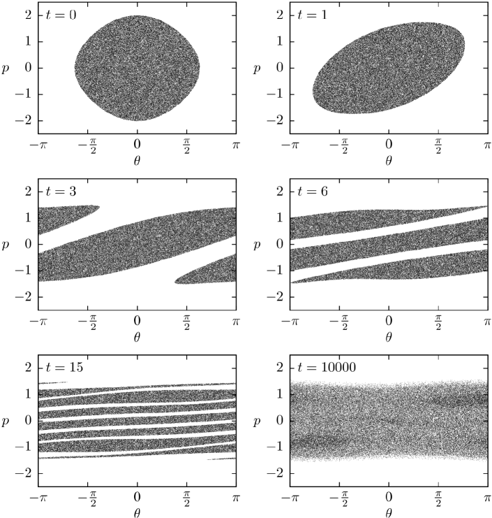
Eventually, the length scale of the dynamical evolution will become so small, that to an observer it will appear that the dynamics has ceased. At this stage, we may say that the coarse-grained distribution, , has achieved a stationary state, even though the fine-grained distribution is still evolving. For a practical purpose of describing the results of molecular dynamics simulations — which, of course, have finite precision — we only need to have the knowledge of .
3.1 Lynden-Bell Statistics
In a seminal work, Lynden-Bell (LB) proposed a statistical approach for calculating for the final stationary state [104]. LB theory is similar in its construction to the usual Boltzmann statistics, but instead of working with the particles, Lynden-Bell studied the distribution of the phase space density levels, . It is important to keep in mind that, similar to the usual equilibrium statistical mechanics, the LB approach requires the existence of ergodicity and mixing [100, 7].
The phase space is divided into macrocells which are in turn subdivided into microcells of volume . As the dynamics progresses, the distribution function spreads over the phase space, occupying more macrocells than it did initially. This process is illustrated in Fig 2. The volume fraction occupied by the level inside the macrocell is
| (10) |
where is the number of microcells inside a macrocell occupied by the level . The volume fraction is related to the distribution function by . Due to the incompressibility of Vlasov dynamics, each microcell can be occupied by at most one level , so that the density must satisfy
| (11) |

LB supposed that in a stationary state the dynamics of the density levels is ergodic — ’s have an equal probability of occupying any of the microcells. He then applied the usual Boltzmann counting to calculate the most probable distribution of the density level over the phase space.
The total number of occupied microcells,
| (12) |
remains constant throughout the dynamics. The number of ways in which these microcells can be divided among the macrocells is given by
| (13) |
Now consider a macrocell. The number of ways in which of its microcells can be occupied by a density level is
| (14) |
Note that the density levels are treated as distinguishable. Multiplying expressions (14) and (13) we obtain the total number of possible microstates,
| (15) |
The coarse-grained entropy of the system is defined as where is the Boltzmann constant. In the limit in which the variations of between the macrocells are infinitesimal, the entropy can be written as
| (16) |
Similar to the usual thermodynamic equilibrium, LB proposed that the SS of a LR system corresponds to the most probable distribution of the density levels among the macrocells. To find this distribution, we must maximize the LB entropy under the constraints of energy
| (17) |
and particle
| (18) |
conservation. In the above equations is the average particle energy in the initial distribution and is the potential at position in the stationary state. Maximizing the entropy Eq (16), under the constraints given by Eqs. (17) and (18), we find the coarse-grained distribution function for the SS,
| (19) |
where is the one-particle energy. The Lagrange multipliers and are the inverse temperature and the chemical potential of the stationary state. The expression (19) is similar to the distribution function of fermions in an equilibrium system.
Besides Lynden-Bell’s theory, other statistical approaches have also been proposed to study qSSs which arise in the process of collisionless relaxation. Example include, statistics based on particles instead of the distribution function [105] and an information-theoretical approach [106, 102]. Just like LB theory these approaches require existence of ergodicity and good mixing [107, 108] which, in general, are not valid for systems with LR forces. In this Report, we will only focus on LB theory. In the following sections we will see how well it compares with the simulations.
4 Gravitation in one dimension
Due in part to complications of 3D gravitational systems, which will be addressed later on, many studies of self-gravitating systems have focused on one and two dimensions [109, 110, 30, 111, 112, 113, 34, 114, 115, 116, 117, 118]. The reduced dimensionality makes the study of these systems much simpler. The fact that the gravitational potential in one and two dimensions is unbounded from above prevents particle evaporation which makes theoretical and simulation work on 3D systems very difficult. In spite of their greater simplicity, 1D and 2D gravitational systems share many characteristics of 3D gravity. For example, the global structure of disk-like galaxies, found using 3D numerical simulation, are also reproduced by 2D simulations [79]. One-dimensional self-gravitating systems have also been used to study the stellar dynamics of galaxy clusters and of cosmological models [58, 59, 28, 119, 120, 31, 121, 122, 123, 124, 125, 126, 118, 127].
A 1D self-gravitating system consists of sheets of mass density uniformly distributed in the – plane, free to move along the axis. The dynamics of the sheets is the same as the dynamics of point particles of mass interacting by a linear potential. The particles are free to cross one another. The thermodynamic limit, , is equivalent to the Kac prescription necessary to guarantee the extensivity of the energy.
The Poisson equation for this system is
| (20) |
where is the gravitational constant and is the mass density. In order to simplify the expressions, we will work with dimensionless variables. We shall rescale the mass, length, velocity, potential, and energy222A system’s energy takes into account the total work necessary to bring a particle from infinity (or from a position where the potential is zero) to a position , i.e. . For 3D self-gravitating systems the potential at infinity is zero, and for plasmas it is zero at the conducting wall. However, it is important to note that for 1D and 2D self-gravitating systems, the potential diverges at infinity. Since this divergent term appears in both the initial and the final state, the problem is avoided by using a renormalized energy, see Ref [39] for more details. by , (an arbitrary length scale), , and , respectively. This is equivalent to considering and to defining a dynamical time scale
| (21) |
Thus, the Poisson equation becomes
| (22) |
For a particle (sheet) of (reduced) mass density located at , the density is , and the long-range potential is given by the Green’s function,
| (23) |
A particularly interesting aspect of the one-dimensional gravity is that the interaction potential does not have any singularities, which simplifies significantly molecular dynamics (MD) simulations, allowing us to explore in great detail the relaxation of this model to the qSS.
4.1 Molecular Dynamics
The reduced Hamiltonian for a system of particles interacting by a one-dimensional gravitational potential is
| (24) |
This Hamiltonian, along with Hamilton’s equations of motion, completely determines the dynamics of the system. The acceleration of a particle at position , due to its interaction with the other particles, is given by
| (25) |
which may be expressed as
| (26) |
where and represent the number of particles to the right and to the left of , respectively. To simulate the system according to equation (26) requires time that scales with . However, the simulation may be simplified by using a vector containing the indices of each particle, and reordering it according to each particle’s position at each new calculation. The expression in equation (26) then may be written as
| (27) |
where is the index of the particle at position . This simplification involves no approximation; the advantage is purely computational, for the simulations become more efficient regarding the computational time [128]—the typical time required to order a vector of size varies at most with [129]. Using this method, the trajectories may be obtained exactly, that is, at machine precision [128]. However, for the exact procedure, the trajectories must be calculated at each collision, and the number of collisions grows as . Therefore, in our simulations, we used a fourth-order symplectic integrator, reordering the index vector at each time step and maintaining the relative error in energy at .
We simulate numerically the evolution of a system of particles that are initially distributed uniformly with positions where and velocities , so that the initial distribution function is given by
| (28) |
where . In order to calculate the initial energy, we must find the potential that is the solution of the Poisson equation (22) at ,
| (29) |
with boundary conditions and . The solution is given by
| (30) |
Using the definition of the mean energy, equation (17), the initial energy of the system is found to be
| (31) |
where without loss of generality we have set .
4.2 Equilibrium
If the system relaxes to equilibrium the gravitational potential must satisfy the Poisson equation
| (32) |
where is the equilibrium density distribution. Using the Maxwell-Boltzmann distribution, , the equilibrium density distribution is given by
| (33) |
where is the Lagrange multiplier used to conserve total energy, is the normalization constant and is the potential of mean force [97]. As , interparticle correlations vanish and . Substituting equation (33) into equation (32), we obtain the Poisson-Boltzmann equation in its dimensionless form
| (34) |
Solving this equation using the boundary conditions and , the potential is found to be [120]
| (35) |
and the distribution function is given by
| (36) |
The value of is determined by the conservation of energy, Eq. (17) with , yielding
| (37) |
The equilibrium density and velocity distributions are given by
| (38) |
and
| (39) |
In Fig 3 we compare the equilibrium distributions, Eqs (38) and (39), with the results of MD simulations. As can be seen, the predictions of equilibrium statistical mechanics are very different from those of MD simulations. This clearly shows that the ergodicity required by the Boltzmann-Gibbs statistical mechanics is violated.

In the next section we will compare the predictions of Lynden-Bell statistics with the results of MD simulations.
4.3 Lynden-Bell theory for one-dimensional gravity
The application of Lynden-Bell statistics to one-dimensional gravitational systems has spanned various decades, with divergent results. While early studies have suggested some correspondence between numerical simulations and the predictions of LB statistics, especially for low-energies, they have also shown the occurrence of high-energy tails in the distribution, which LB statistics could not describe [29, 130, 131, 132, 133]. The more recent works demonstrated that although for some very specific initial conditions LB theory agrees well with MD simulations, in general it fails to describe the qSS [134, 108, 135, 123]. In this section we will examine the predictions of LB statistics and compare them with the results of MD simulations for various initial conditions.
In order to determine , Eq (19), for a one-dimensional gravitational system, we need to calculate the gravitational potential . To do this we must solve the Poisson equation (equation (22)) with and the one-particle energy given by . Integrating the LB distribution over momentum, we obtain the Poisson equation
| (40) |
with boundary conditions and , where is the polylogarithm function of order [136]. The solution to this equation is obtained numerically. We see that the predictions of LB statistics are in general quite different from the results of MD simulations, as exemplified in Fig 4, which compares the position and the velocity distributions and with the results of MD simulations.

The problem, common to both BG and LB statistics, is that in thermodynamic limit, systems with LR forces are intrinsically non-ergodic, invalidating the basic assumptions that underlie both theories. For systems with a finite number of particles, however, ergodicity is restored on a sufficiently long time scale. Such systems will eventually relax to the BG equilibrium (if it exists, and the BG entropy has a maximum), after being trapped in a qSS for a time proportional to the number of particles in the system.
The Kac scaling required by the LR nature of the interaction potential destroys the correlations (collisions) between the particles [97]. Therefore, in thermodynamic limit, LR systems are intrinsically collisionless – particles move under the action of the mean-field potential produced by all the other particles. In general, the mean-field potential has a complex dynamics, characterized by quasi-periodic oscillations [121]. It is possible, therefore, for some particle to enter in resonance with the oscillations and gain large amounts of energy at the expense of the collective motion [137, 46, 138]. This process is known as Landau damping [139]. The Landau damping diminishes the amplitude of the oscillations and leads to the formation of a tenuous halo of highly energetic particles which surround the high density core [140]. After all the oscillations have died out, a SS state is established. The phase space distribution of particles in the qSS has a characteristic core-halo structure, very different from the predictions of either BG or LB statistics. Once the stationary state is established, there is no longer a mechanism through which highly energetic particles of the halo can equilibrate with the particles of the core, and the ergodicity is broken.
4.4 The virial condition
If the system is in a stationary state, it must satisfy the virial theorem. Consider a system with a Hamiltonian given by
| (41) |
where are respectively the coordinates of position and momentum of the th particle, is the interaction potential and is a generic confining potential. The virial function is defined as
| (42) |
where represents a time average. Differentiating the virial function with respect to time and using Hamilton’s equations [141], we find
| (43) |
where
| (44) |
If is a homogeneous function of order , that is, , then by Euler’s theorem,
For a stationary state, , which determines the virial condition
| (45) |
where is the average kinetic energy per particle in a SS, is the average potential energy per particle in a SS, and . In the case of two-dimensional gravity333The specific case of two-dimensional gravity is addressed in Ref [142], which presents a study of the virial theorem in the general case of dimensions and includes terms for friction and noise., which will be discussed in section 5, the interaction potential is logarithmic, , and is not a homogeneous function. However, writing the logarithm as , after some manipulation (see [39]), we find
| (46) |
Using equation (46) in equation (43), the virial condition for a 2D gravitational system is found to be
| (47) |
where we have set in equation (41).
In 1D the gravitational potential is a homogeneous function of order , so that the virial condition reduces to
| (48) |
If at the initial distribution function is not a stationary solution of the Vlasov equation, the system will undergo oscillations. When the relaxation is completed and a qSS is established, equation (48) must be satisfied. However, even if the initial distribution function does not satisfy the stationary Vlasov equation — as is the case for the waterbag distributions considered above — we can significantly diminish the amplitude of oscillations during the relaxation process if the initial distribution is forced to satisfy the virial condition, Eq (48). For such distributions, even though the initial state is not stationary, it is not “too far” from a qSS. To quantify this, we define the virial number for 1D gravity as . When , the virial condition is satisfied and the oscillations should be suppressed; on the other hand, if , the system will experience strong density oscillations due to the imbalance between the kinetic and the potential energies. We expect that the process of relaxation to the qSS should be quite different for these two cases.
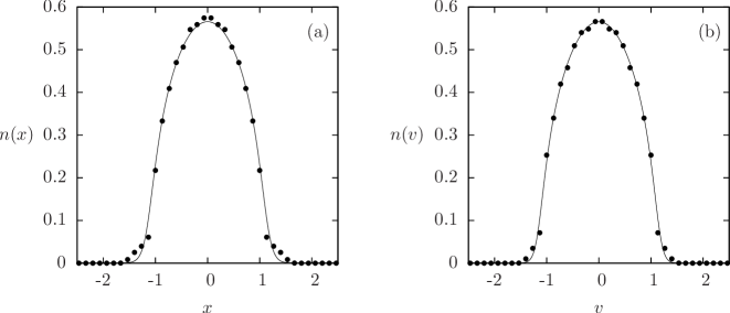
Indeed, we find that when , where is the virial number at time , the resulting qSS has a compact structure, which is reasonably well captured by LB theory, see Fig. 5. On the other hand when , the system separates into a central core surrounded by a halo of highly energetic particles. To understand the mechanism of the core-halo formation we need to explore the parametric resonances which appear as a result of the density oscillations.
4.5 Envelope equation
To explore the density oscillations, we define the envelope to be the initial size of the system, . Note that at , the envelope coincides with the boundary of the initial waterbag distribution, . Differentiating twice with respect to time, we have
| (49) |
To simplify the first term, we suppose that the mass density oscillations are smooth, so that the particle distribution remains uniform. Under these conditions, the oscillating gravitational potential maintains the functional form given by Eq. (30), but with ,
| (50) |
Similarly, the distribution function will be approximated by a waterbag
| (51) |
with . The average can then be expressed as
| (52) |
resulting in
| (53) |
The second and the third terms of Eq. (49) are
| (54) |
and
| (55) |
considering that at there is no correlation between position and velocity. The envelope equation reduces to
| (56) |
where and the initial conditions are and . If , then , and the system does not develop oscillations. Fig 6 compares the oscillations of the envelope predicted by Eq (56) with the results of MD simulation, showing a reasonable agreement for short times.

4.6 The test particle model
To understand the mechanism of halo formation, we first study the dynamics of noninteracting test particles initially located at positions with velocities , where . Each particle moves in a gravitational potential produced by the oscillating mass density
| (57) |
where is governed by the envelope equation, Eq (56). The trajectory of a test particle is then determined by the equation of motion
| (58) |
where is the sign function [143].

In Fig 7 we show the Poincaré sections for test particle dynamics. When , the trajectories of the test particles correspond to harmonic oscillators and the dynamics is completely regular; on the other hand, when , we see the appearance of resonance islands. At short times a very similar structure of the phase space is also found in the complete MD simulation, as shown in panel (c) of the same figure. The formation of resonance islands is the result of the particle(density)-wave interactions [144, 145, 146]. The parametric resonances allow some particles to move into the regions of the phase space which are highly improbable from the perspective of BG or LB statistics. Once the oscillations die out, these particles are trapped, becoming a part of a halo.
4.7 The core-halo distribution
From the Jeans theorem, a steady-state solution of the Vlasov equation depends on the phase space coordinates only through the integrals of motion of the mean-field potential. Conversely, any function of the integrals of motion is a steady-state solution of the Vlasov equation [64]. In all the cases treated in this Report, the only integral of motion is the one-particle energy. Thus, a Maxwell-Boltzmann distribution is only one of the infinite number of solutions of the Vlasov equation. In particular an arbitrary initial distribution will not converge to the Maxwell-Boltzmann distribution, as is the case for systems with finite-range forces.
Unlike gravitation in three dimensions, in 1D particles cannot escape to infinity. The test particle dynamics shows, however, that the resonant particles may gain a lot of energy from collective oscillations and form a tenuous high-energy halo that surrounds the central core region. Since the Hamiltonian dynamics is conservative, the gain of energy of resonant particles must result in the loss of energy (cooling down) of the core particles. In principle, the halo formation will continue until the oscillations of the core have completely died down. Once the SS state is established, the core particles should be in the "ground state". The incompressibility constraint imposed by the Vlasov dynamics, however, does not allow the core particles to collapse to the minimum of the potential energy. Rather, these particle will arrange in such a way as to occupy all of the low energy states up to the allowed maximum phase space density ,
| (59) |
where is the "Fermi energy" of the core.
The maximum energy that a halo particle can gain corresponds to the resonant orbit. As the oscillations die down, the resonances shift toward the smaller energies, resulting in a quasi-homogeneous population of the phase space between and the maximum halo energy, . We will, therefore, suppose that in a qSS the halo particles are distributed according to
| (60) |
where is the phase space density of the halo particles and the maximum halo energy, , can be calculated using the test particle dynamics and is given by , see Fig 7. The complete core-halo distribution is then
| (61) |
From now on, for simplicity we will write instead of . After determining using the test particle dynamics, two unknowns remain, and , which are obtained using the conservation of the total energy and the number of particles in the system. Integrating the core-halo distribution function over velocities and substituting the resulting particle density into Poisson equation, the gravitational potential is found to satisfy
| (62) |
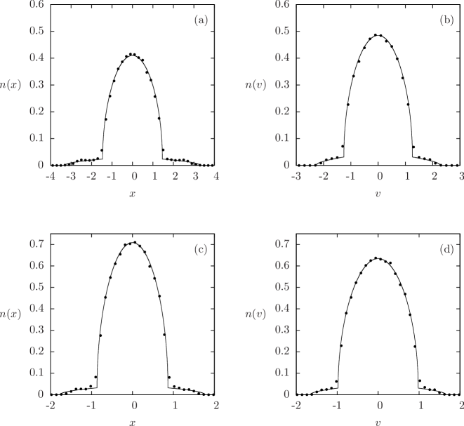
with the boundary conditions given by and . The parameters and are determined self-consistently from the numerical solution of equation (62) and the conservation of the total energy and the number of particles (equations (17) and (18)) in the system. Once the potential is known we can easily calculate the distributions and , see Fig. 8.
4.8 Thermodynamic equilibrium
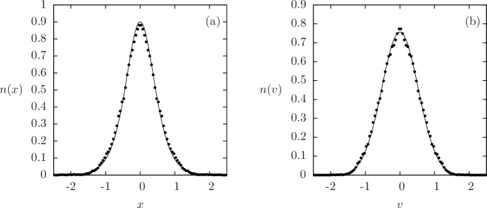
For finite , correlations are not completely negligible and eventually they will drive the system to thermodynamic equilibrium. The equilibrium state should be described by the MB distribution Eq (36), discussed in subsection 4.2. Therefore if the number of particles in the system is not too large and the simulation is run for a sufficiently long time the thermodynamic equilibrium should be observed. Figure 9 shows the results of MD simulation for . We see that after this time the system indeed relaxes to the thermodynamic equilibrium with the particle distribution given by Eq (36).
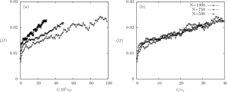
The approach to equilibrium can be observed using a crossover parameter, , which measures how well the system’s density profile is described by the core-halo distribution , Eq (61) at each instant. We define
| (63) |
where is the number of particles located between and at time and . The smaller the value of , the better the agreement between the system’s marginal distribution in position and the predicted distribution of the core-halo theory. When the system starts to cross over to equilibrium, begins to deviate from its minimum, growing until it reaches the equilibrium value, given by where with given by Eq (38). In Fig 10, we show the evolution of for different values of . After relaxing to the qSS, rises and approaches the equilibrium value. Rescaling time with , with , all the curves collapse onto one universal curve. This value of is approximate — to find a precise value of , a very large number of particles must be used in MD simulations. Nevertheless, the observed value of agrees quite well with the exponent predicted by the theoretical argument of Section 2. While our simulations find , other previous simulations with smaller number of particles find [111], [147] and greater [31, 32, 148].
5 Gravitation in two dimensions
We next consider self-gravitating systems in two dimensions. Such systems and their dynamics have been applied to study topics ranging from the spiral structure of disk-like galaxies [109, 110, 149] to the large-scale structure of the universe [150]. They have also been analyzed in the context of equilibrium thermodynamics [151, 152].
The system consists of particles of mass in a two-dimensional space. The total mass of the system is . It is convenient to define dimensionless variables by rescaling length, velocity, potential, and energy with respect to (an arbitrary length scale), , and , respectively, where is the gravitational constant. This process is equivalent to setting and to defining the dynamical time
| (64) |
In three-dimensional space, the system corresponds to rods of mass density [151].
Considering only systems with azimuthal symmetry, the corresponding gravitational potential satisfies the dimensionless Poisson equation,
| (65) |
where is the mass density of a self-gravitating system which is obtained from the one particle distribution function, . For an isolated particle the density is
| (66) |
so that the Green’s function solution to Eq (65) is
| (67) |
The Hamiltonian for a particle gravitational system is then
| (68) |
5.1 Molecular dynamics
We will study 2D gravitational systems in the thermodynamic limit. In this limit, if the initial distribution is azimuthally symmetric, the mean-field potential will also retain this symmetry, so that the angular momentum, , of each particle is conserved. This allows us to use an effective Hamiltonian description based on the Gauss’s law. A particle at position is subject to an interaction potential produced by all the particles with , leading to an effective Hamiltonian
| (69) |
where
| (70) |
is the mass of all the particles with the radial coordinates . The equation of motion for is then
| (71) |
where is determined by the initial distribution. The advantage of the effective Hamiltonian is that the simulation time of the system’s dynamics depends exclusively on the time of sorting a vector composed of elements, similar to 1D gravity.
At the start of the simulation the point particles are distributed uniformly inside a circle of radius . They are also assigned velocities from a uniform distribution with the maximum value . This corresponds to a one-level initial distribution of the form
| (72) |
where is the normalization constant.
Since in the thermodynamic limit the mean-field potential is purely radial, the angular momentum of each particle will remain constant throughout the simulation. The radial dynamics of each particle is then determined by the Eq (71), while the dynamics is controlled by the angular momentum conservation . The magnitude of the velocity of the particle is .
The potential associated with the initial distribution satisfies the Poisson equation,
| (73) |
with the boundary conditions given by and . The solution to this equation is
| (74) |
Using this potential, Eq (74), and the initial distribution function, Eq (72), in the expression for conservation of energy, Eq (17), the initial energy of the system is calculated to be
| (75) |
where without loss of generality we have set .
We now consider two cases: one in which the initial distribution obeys the virial condition () and one in which it does not (). In section 4.4, we have shown that the virial condition for a two-dimensional gravitational system requires that . In the thermodynamic limit, using the rescaled variables, the virial condition reduces to
| (76) |
We then define the virial number for a 2D gravitational system to be
| (77) |
5.2 Lynden-Bell theory for a 2D self-gravitating system
In analogy with 1D gravity, if the initial distribution of a 2D self-gravitating system obeys the virial condition, we expect that the parametric resonances will not be excited and the qSS should be well described by the Lynden-Bell statistics. The mean-field potential should then satisfy the Poisson equation with the mass density given by the momentum integral of Eq (19),
| (78) |
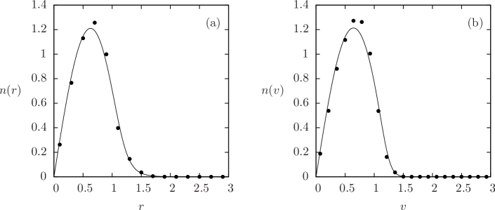
The boundary conditions for this equation are and . The parameters and are determined self-consistently by the conservation of energy and norm of the distribution function, Eqs (17) and (18). Once , , and are calculated, we can compare the theoretical predictions with the results of the MD simulations. To do this we calculate the marginal distributions: the number of particles located between ,
| (79) |
and the number of particles with velocities between ,
| (80) |
Comparing the theory and the simulation, we see a reasonably good agreement between the LB statistics and the results of MD simulations, Fig 11.
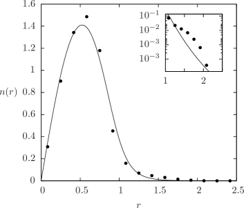
However, if the initial distribution does not satisfy the virial condition, LB theory starts to deviate from the results of MD simulations. A tail in the marginal distribution functions emerges, showing the formation of a core-halo structure, see Fig 12.
5.3 The envelope equation
The appearance of the core-halo structure is a consequence of the parametric resonances which arise from the density oscillations. To study these oscillations we define the envelope of the particle distribution as . Note that with this definition . Differentiating twice with respect to time, we find
| (81) |
which can be rewritten as
| (82) |
where
| (83) |
is known as the “emittance”. The emittance is an important parameter in the physics of charged particle beams, and is related to the area occupied by the particles in the phase space [75]. Unlike the one-dimensional case, in two dimensions the term can be simplified using the Poisson equation (65),
| (84) | |||||
The gradient of the potential at is , and we obtain
| (85) |
We are interested to study the behavior of a 2D self-gravitating system when its initial distribution does not deviate significantly from the virial condition. In this case, we expect that the emittance will remain close to its initial value, , so that the envelope equation reduces to
| (86) |
As expected, if and , , so that the envelope does not develop oscillations.
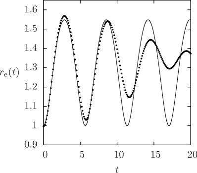
Comparing the temporal evolution of with the data from MD simulations, we see that there is a reasonably good agreement between the two, especially for short times (Fig. 13).
5.4 The test particle model
We now study the behavior of test particles subject to a gravitational potential produced by an oscillating uniform mass distribution,
| (87) |
Solving the Poisson equation we find
| (91) |
This means that the dynamics of a test particle which at was at and had an angular momentum will be governed by the equation of motion
| (95) |
where is the solution of Eq (86).
We integrate the equations of motion (95) for test particles, uniformly distributed at , and , with . The Poincaré section is constructed by plotting the position and velocity of each test particle when the envelope is at its minimum value, see Fig. 14.
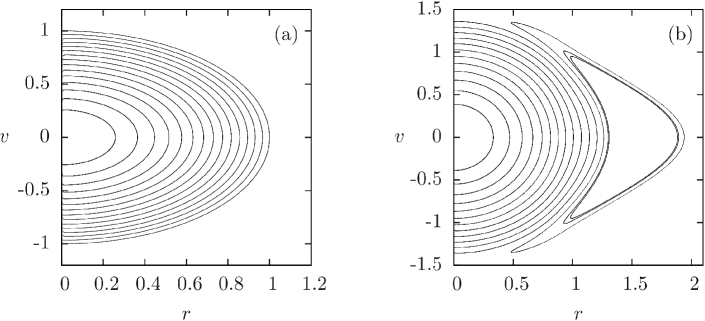
In Fig. 15 we compare the phase space structure of the test particle dynamics to a snapshot of the phase space obtained using MD simulation, after the qSS has been established.
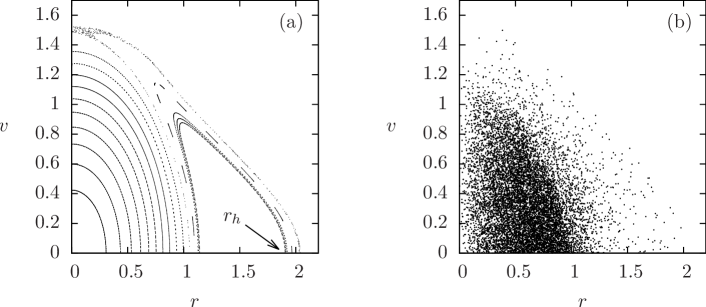
We see that the test particle dynamics allows us to calculate the maximum energy that a particle of a self-gravitating system can gain from the density oscillations.
5.5 Core-Halo Distribution
The particles which enter in resonance with the core density oscillations escape from the central region producing a tenuous halo. The halo formation progressively dampens the oscillations, bringing the resonances closer and closer to the core. When the qSS is established, we expect that the particle distribution will, once again, correspond to the core-halo distribution, given by
| (96) |
where and are calculated using conservation of energy and norm and is determined by the test particle dynamics, see Fig 15. Integrating the core-halo distribution over , we obtain the particle density in the qSS state. Substituting this into Poisson equation (65), we obtain the equation for the gravitational potential of a 2D cluster
| (102) |
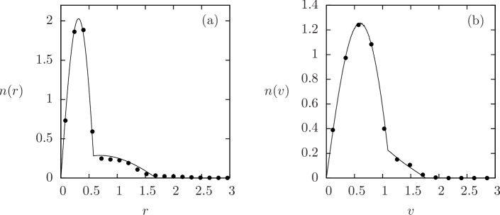
with boundary conditions and . The system of equations (102) can be solved analytically, see Ref [39]. Comparing the marginal distributions predicted by the core-halo theory to the results of MD simulations (Fig. 16), an excellent agreement between the two is observed.
5.6 Relaxation time
Finally, it is interesting to explore how much time a finite system of particles remains in the qSS before relaxing to the true thermodynamic equilibrium. To this end, we use the crossover parameter , defined as
| (103) |
where is the number of particles located inside shells between and at time and , where is the core-halo distribution, Eq (96).
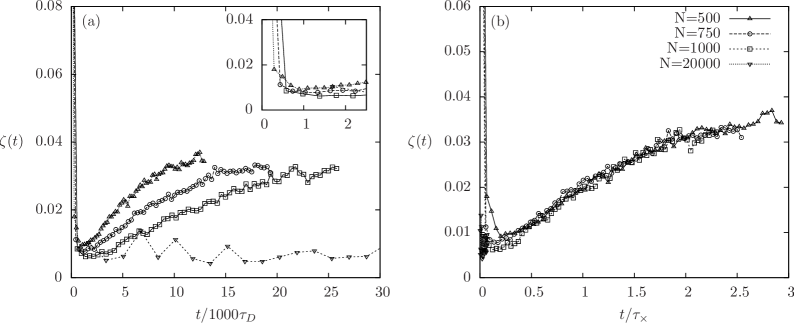
Figure 17 shows the value of for systems with different numbers of particles. The panel 17b shows that if the time is rescaled by , where and is the dynamical time defined by Eq (64), all the curves fall on a universal curve, indicating the divergence of the crossover time in the thermodynamic limit. Thus, in the limit a self-gravitating system will remain forever trapped in a nonequilibrium stationary state. Recent simulations performed with discrete particles instead of the concentric shells used in this Report have lead toexponent, [153], which is in good agreement with the scaling argument presented in Section 2, .
5.7 Thermodynamic equilibrium
For a finite number of particles, after a time , we expect the system to relax to thermodynamic equilibrium, with
| (104) |
where is the normalizations constant. To see that this is the case, we calculate the gravitational potential and the marginal distributions and compare them to the results of MD simulations. The gravitational potential in equilibrium will satisfy the Poisson-Boltzmann equation
| (105) |
where is the Lagrange multiplier used to enforce the conservation of the total energy. The solution of this equation is given in Ref. [39],
| (106) |
Curiously, an isolated 2D gravitational system can only exist at one temperature, , independent of the initial energy. If such a system is put in contact with a thermal bath, it will either gain energy from the bath and grow without bound or lose energy and shrink, depending if the temperature of the bath is greater or smaller than , respectively.
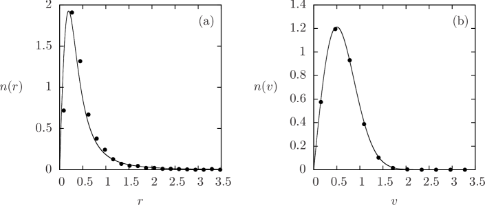
Figure 18 compares the marginal distributions obtained using the MD simulations with the predictions of equilibrium statistical mechanics. The number density of particles located between is
| (107) |
and the number density of particles with velocities between is
| (108) |
The figure shows a good agreement between the results of MD simulations and BG statistics. However, to reach thermodynamic equilibrium, it was necessary to run a simulation with particles for dynamical times. Up to this time, the system remained trapped in a qSS state with the particles distributed in accordance with the core-halo distribution function , Eq (96).
6 Gravitation in three dimensions
The relaxation of 3D self-gravitating systems is extremely difficult to study. There are two basic problems arising from the fact that Newton’s gravitational potential has no lower bound, but is bounded from above. The consequence of the upper bound is that some particles of a self-gravitating system can gain enough kinetic energy to escape the gravitational field of the cluster. In principle, there is no limit to the particle evaporation since the energy can be constantly supplied by the two-body collisions [61, 101, 38] and the gravitational collapse. As a consequence, the Poisson-Boltzmann equation for a 3D open system has no solutions. Based on cosmological simulations, however, it has been observed that 3D systems do relax to qSSs [154, 155, 156]. There have been a number of phenomenological models proposed to describe the observed density profiles in such qSS: “de Vaucouleurs”, “Sérsic” and “NFW” models [157, 158, 159, 160, 161, 162, 163]. These, phenomenological density distributions, however, lack the theoretical foundation.
The fact that the Poisson-Boltzmann equation does not have a solution indicates that open 3D self-gravitating systems are intrinsically unstable in the infinite time limit. This instability, is a consequence of the the binary collisions which lead to a flux of evaporating particles. On shorter time scales, however, it is possible for a system to relax to a collisionless qSS. Again, however, the situation in 3D is much more complex than in one and two dimensions [109, 110, 30, 111, 112, 113, 34, 114, 116, 117, 118]. Significant evaporation of particles can happen even on very short time scales, leading to a halo that extends all the way to infinity. At the moment, there is no theory that can account for the particle distribution inside a 3D halo. The theory of parametric resonances, which was so successful for treating 1D and 2D gravity, can not be applied in 3D since, in general, there are no bounded resonant orbits.
Although the particle distribution in a qSS can not be predicted a priori, we expect that it will have a core-halo structure. Evaporation should progressively cool down the core region. Statistically only a completely degenerate core can remain stable in an infinite space — at finite temperature the entropy gain will always favor particle evaporation. Furthermore, since the collisionless relaxation is controlled by the Vlasov equation, the phase space density in the core can not exceed that of the initial waterbag distribution. We, therefore, expect that the core will be described by a fully degenerate Fermi-Dirac distribution [38] with the "spin" degeneracy equal to the phase space density of the initial waterbag distribution. The difficulty, however, is that without knowing the full particle distribution in the halo, we can not calculate the self-consistent gravitational potential and close all the equations of the theory.
For a 3D gravitational system of total mass , the gravitational potential in the qSS must satisfy the Poisson equation,
| (109) |
where is the one particle distribution function. If the potential has a radial symmetry, the particles can be represented as spherical shells of mass . This approach greatly facilitates the numerical simulations, and becomes exact in the thermodynamic limit.
It is convenient to measure all the distances in an arbitrary length unit , the time in units of dynamical time,
| (110) |
and the gravitational potential in units of . The Poisson equation (109) then reduces to
| (111) |
For a particle located at , , the Green’s function of Poisson equation is the usual Newton’s gravitational potential
| (112) |
This potential diverges at small distances and is bounded from above. We saw already that in 1D and 2D some particles enter in resonance with the density oscillations and gain a lot of energy. The situation in 3D is even more complex — the potential is bounded from above so that the resonant particles can gain enough energy to completely escape from the gravitational field of the cluster.
6.1 Test particle dynamics
To get a better idea of the relaxation process which leads to the core-halo formation, we study the dynamics of test particles moving under the action of an oscillating gravitational potential. Once again we consider particles which at were distributed uniformly in the phase space inside a sphere of radius and . We define the "envelope radius" as , which at satisfies . We will work in dimensionless units and set . Differentiating twice with respect to time and performing manipulations similar to those for 1D and 2D gravitational systems, we obtain a differential equation that governs the envelope dynamics,
| (113) |
where
| (114) |
is the virial number, and and are the kinetic and the potential energy of the initial distribution.
We consider the dynamics of test particles, initially distributed uniformly with positions and velocities ,
| (118) |
where and evolves according to Eq (113).
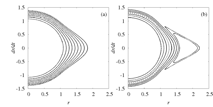
Fig 19 shows the the Poincaré sections for two systems with and . For , the orbits remain integrable, while even a small deviation from the virial condition results in the appearance of a resonance island. For slightly larger or smaller the resonant orbit becomes unbounded.
6.2 Lynden-Bell theory for a 3D self-gravitating system
It is interesting to consider the predictions of the LB theory for a 3D self-gravitating system. In this case the one-particle distribution function becomes
| (119) |
where and . Integrating over the velocities we obtain the density distribution corresponding the the LB stationary state. Substituting this into the Poisson equation allows us to write a self-consistent equation for the gravitational potential
| (120) |
where is the polylogarithm function of . This equation has to be solved numerically and the two Lagrange multiplier and must be calculated to preserve the number of particles and the energy of the system. The solution of Eq (120) is complicated by the open boundary conditions. In practice, we will solve this equation by enclosing the system in a spherical box of radius and then take the limit .


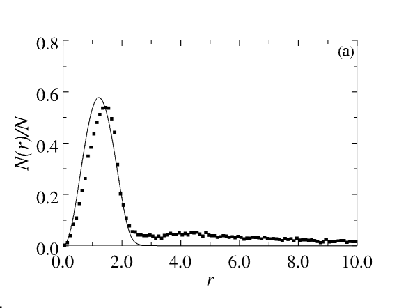
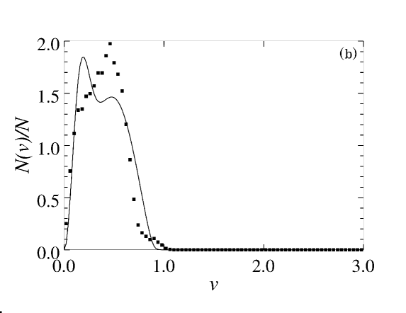
As expected, when , the LB distribution separates into a completely degenerate core and a very tenuous halo which extends all the way to . However, the particle distribution in the halo is very different from the ones found in MD simulations, see Fig. 21, so that LB theory fails to correctly describe a 3D self-gravitating system.
.
6.3 Systems with
If the initial particle distribution satisfies the virial condition , the macroscopic oscillations will be suppressed and the parametric resonances will not be excited, see Fig. 19. For such initial distributions, we saw that LB theory worked reasonably well for 1D and 2D gravitational systems. For 3D systems, however, LB theory fails even when . As , the solution of Eq (120) requires that (see Fig 20) and the distribution function approaches the degenerate limit (plus halo particles at infinity). Thus, for an open system, LB theory will always predict a fully degenerate core [164]. This conclusion, however, is valid only in the asymptotic limit. In this limit, even small oscillations of the envelope will lead to particle evaporation and result in formation of a cold core. In practice, however, for the rate of evaporation is very low, so that the degenerate limit will not be reached in the time of simulation. To treat this “short” time limit, we can introduce an effective cutoff (a wall) at . The precise value of the cutoff is unimportant — as long as it is not too large . The wall will prevent the particle evaporation and a complete cooling of the core region. Indeed, the cutoff-LB distribution (cLB) is found to describe reasonably the qSS state for [38], see Fig. 22


7 Non-neutral plasmas
In this chapter we will analyze qSSs of magnetically confined non-neutral plasmas. The non-neutrality condition is crucial for the plasma to be a long-ranged interacting system — for neutral two component plasmas, Debye screening leads to an effective short-range interaction potential [165, 166, 75]. Equilibrium state of neutral plasmas and electrolytes, therefore, can be studied using the usual Boltzmann-Gibbs statistical mechanics [97].
Many different applications, such as heavy ion fusion, high-energy physics, communications, materials processing, and cancer therapy, depend on the physics of transport of intense charged-particle beams. The goal is to avoid the heavy particle losses produced by the parametric resonances [47, 167], which can lead to halo formation that is detrimental to the beam quality, and can result in damage to the accelerator walls. A theory which can quantitatively predict this effect is, therefore, highly desirable for a better understanding of the physics of beam transport [140, 168, 50, 169, 170].
In general, the dynamics of the beams is influenced by multiple effects, including the mismatched envelope (rms radius of the beam) [140, 51, 52, 171, 50], movement outside the axis of symmetry [172, 173, 174, 175, 176, 177], nonuniformities in the beam distribution [178, 179, 180, 145], and the image forces due to the surrounding conducting walls [181, 182, 183]. Of all these, the study of parametric resonances resulting from the transverse beam oscillations has attracted the most attention. Envelope mismatch is believed to be the main cause of the halo formation in space-charge dominated beams [184]. In this section we will show that the mismatch of the beam envelope is closely related to the virial condition — similarly to the one found for self-gravitating systems — and that the final qSS is, once again, described by the core-halo distribution function.
7.1 The model
Our system consists of a beam of charged point particles, confined by an external magnetic field , propagating along the axial direction, with velocity . The beam has a characteristic radius and is surrounded by a conductive cylindrical wall of radius 444A conducting grounded wall requires that the electric potential at the wall vanishes ..
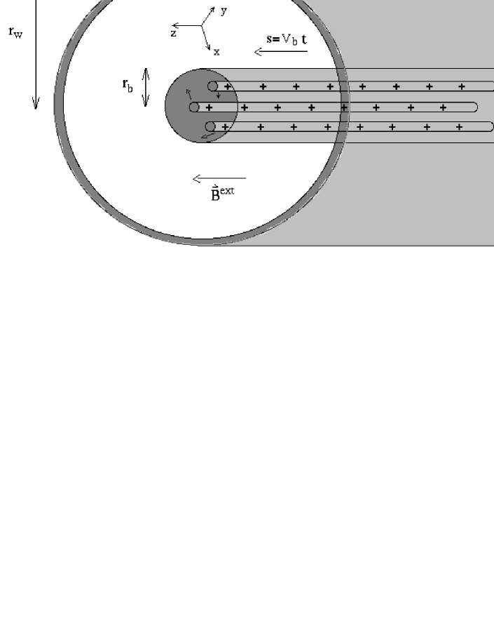
We assume that the beam has axial symmetry and that the motion along the direction is uniform. Consequently, we consider that the relevant dynamics takes place only in the transverse plane “”555We approximate since the variation of the potential along the longitudinal direction is negligible compared to the variations in the transverse plane. Therefore, in this section, will be understood to represent .. Under these conditions, the time can be replaced by the longitudinal coordinate , by means of a canonical transformation of the original Hamiltonian, where and , being the speed of light in vacuum, as illustrated in Fig 23.
The charge of the beam particle is , where is the valence and is the electron charge. Furthermore, assuming that the transverse velocity of the beam particles is much lower than the longitudinal velocity, the dynamics along the transverse plane may be considered non-relativistic. This set of conditions, known as the paraxial approximation, is sufficient to study narrow and intense charged-particle beams [75].
The electric and magnetic fields satisfy Maxwell’s equations [75] and the electric potential the Poisson equation,
| (121) |
with boundary conditions and , where is the number density of the particles. The electric potential is always zero outside the conductive wall, located at . The vector potential, , produced by the current of charges — the longitudinal velocity of the beam, , is approximated by — satisfies
| (122) |
Comparing equations (121) and (122), we see that the electric and vector potentials are related by
| (123) |
Thus, solving the Poisson equation (121), we find the electromagnetic field acting on each particle,
| (124) | |||
| (125) |
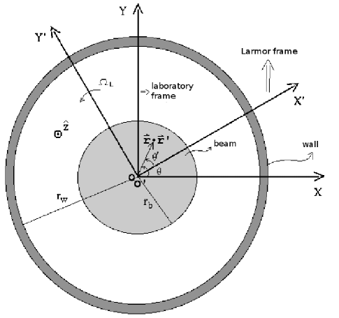
As a matter of convenience, [75, 47], we study the system in the Larmor frame which rotates in relation to the laboratory with a constant angular velocity , where , and is the mass of a particle, see Fig 24. We define the dimensionless potential as
| (126) |
In the Larmor frame, the focusing due to magnetic field , results in a radial confining force. The change to the Larmor frame is accomplished by a change of coordinates , where
| (127) |
as shown in Fig 24. The evolution of the distribution function in the Larmor frame satisfies the Poisson-Vlasov systems of equations [75],
| (128) | |||
| (129) |
where is the density profile of the beam, is the focusing field parameter, and is the perveance which measures the intensity of the beam. The number of particles per unit axial length is , is the position vector in the transverse plane, and is the dimensionless transverse “velocity”. The problem then reduces to studying the dynamics of 2D pseudo-particles of charge confined by an external parabolic potential . The interaction potential between the particles is where is the Green’s function of the two-dimensional Poisson equation. For conducting boundary conditions at , the Green’s function can be calculated using Kelvin’s inversion theorem [185, 143]. The Hamiltonian for the effective 2D system is then
| (130) |
Starting from an arbitrary initial distribution, the system of particles can now be simulated to obtain the final qSS.
If the system has azimuthal symmetry, the simulations can be simplified further. In the thermodynamic limit the Vlasov mean-field description becomes exact, so that each particle moves under the action of the mean-electromagnetic potential produced by all the other particles. To approach the mean-field limit with a finite number of particles we can uniformly smear the charge of each particle over a circle or radius corresponding to its position. This is the same approximation that was used to efficiently simulate 2D and 3D gravitational systems. Using Gauss’s law, the equation of motion for the radial coordinate of a particle becomes
| (131) | |||
| (132) |
where is the number of particles with and . Since the force acting on each particle is radially symmetric, is a conserved quantity determined from the initial condition, . The effective Hamiltonian in the mean-field limit can then be written as
| (133) |
7.2 The envelope equation
We define the beam envelope as . Differentiating twice with respect to gives us the beam envelope equation,
| (134) |
where is the emittance, Eq. (83). This equation is exact; however, the dynamics of is unknown. For short times we will set it equal to the initial emittance .
The beam envelope will not oscillate if . This defines the matched beam radius,
| (135) |
which is equivalent to the virial condition, Eq (45).
If the initial beam is launched with the radius , it will not develop significant oscillations and will not suffer emittance growth. However, in practice it is virtually impossible to launch a beam precisely at this radius. We, therefore, define the virial parameter as
| (136) |
which measures how far the initial beam deviates from the virial condition.
7.3 Initial conditions
At the particles are distributed uniformly in phase space with and velocities ,
| (137) |
It is convenient to measure all length in units and “time” (longitudinal length) in units of . The transverse velocities will then be measured in units . In these dimensionless units the matched beam radius becomes
| (138) |
where . Unlike for self-gravitating systems, for which only the virial number determined the dynamical evolution, in the case of beams we have two dimensionless parameters, and .
In the reduced units, and
| (139) |
where and the emittance growth is .
The potential associated with the initial distribution given by equation (137) can be obtained by solving the Poisson equation (129),
| (143) |
with the boundary conditions and . The solution is
| (147) |
For the initial waterbag distribution (137), the initial energy of the system is
| (148) |
with and defined by Eqs (139) and (136), respectively666If the initial distribution is nonuniform, the functional dependence between and will change..
7.4 Lynden-Bell theory for a charged particle beam
We will first analyze the situation in which the beam envelope at is matched, i.e. satisfies the virial condition . From our experience with self-gravitating systems, we expect that in this case LB statistics should work reasonably well. The electromagnetic potential should then satisfy the Poisson equation (129), with the charge density obtained by integrating the distribution function, Eq (19), over velocities,
| (149) |
The Lagrange multipliers and are determined using energy and norm conservation. The solution to this equation is obtained numerically and the resulting marginal distributions
| (150) |
and
| (151) |
are compared with the results of MD simulations in Fig 25, showing a very good agreement.

7.5 The test particle model
In practice, it is very difficult to launch a perfectly matched beam. In most case and parametric resonances will be excited. To study these, we once again appeal to the model of non-interacting test particles moving in an oscillating potential . We consider test particles initially distributed uniformly with positions and velocities . The equation of motion for the particle is
| (155) |
where evolves according to (134) with .
Comparing the result of the test particle dynamics with the full -body MD simulation, shown in Fig 26, we see that the reduced test-particle model predicts accurately the location of the resonant orbit. This allows us to calculate the maximum energy that a particle can gain from the parametric resonance, , where is the maximum distance from the origin reached by a test particle of the initial distribution, see Fig. 26 (a). Phenomenologically it has been found [50] that for beams with large space charge , is simply related to the virial parameter and the matched envelope radius, .

7.6 The core-halo distribution
For mismatched beams (), we expect that the qSS distribution function will, once again, be of the core-halo type,
| (156) |
It is convenient to divide phase space into three regions, , , and (Fig. 27), corresponding respectively to , , and , where is the core radius.
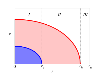
The particle density
| (157) |
in the three regions can be written as
| (158) |
| (159) |
and , where , is the total potential that takes into account the effects of the interaction between particles as well as the contribution of the external field. The parameter is determined by the condition . The maximum halo extent is calculated using test particle dynamics, see Fig 26a. Both and and their first derivatives must be continuous at and . These conditions, together with the Poisson equation (129), provide a closed set of equations for the potential in different regions. The equations can be solved analytically, allowing us to calculate the distribution function in the qSS [186]. A good agreement between theory and MD simulation is shown in Fig 28.

The theory also allows us to predict the emittance growth, a quantity which is of primary importance for beam physics. Comparing the predictions of the present theory with the results of MD simulations, an excellent agreement between the two is observed, Fig. 29. The theory is also in excellent agreement with the experimental measurements [50].
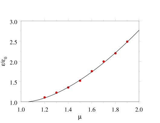
The fraction of particles that escape from the core region to form a high energy halo can be obtained by integrating the distribution function between the energies and , (Fig. 30). We find
| (160) |
where is the modified Bessel function of the first kind of order .

7.7 Relaxation time
Since plasmas contain astronomical numbers of charged particles, relaxation to Boltzmann-Gibbs thermodynamic equilibrium will not happen on laboratory time scale. From the purely theoretical stand point, however, it is interesting to study what would happen if the number of particles can be reduced. This can be easily achieved on computer, if not in practice. We thus define a crossover parameter
| (161) |
where is the number of particles with velocity in the interval at simulation time , and is given by Eq (151). The LB distribution was used in the definition of because we consider cases where the virial condition was initially satisfied. The value of should tend towards its asymptotic value, , as the system approaches thermodynamic equilibrium. This value is given by
| (162) |
where and is the equilibrium distribution function. The dynamic time scale is set to . If the simulation time is scaled with , where , all curves fall on the same universal curve. This show that in thermodynamic limit the crossover time diverges as (Fig 31). The result is very similar to the one found in self-gravitating systems. Recently a theoretical model based on the Chandrasekhar collisional mechanism has been proposed to account for such large crossover time. The theory predicts that the most important factor in determining the exponent is the system dimensionality [187, 188].
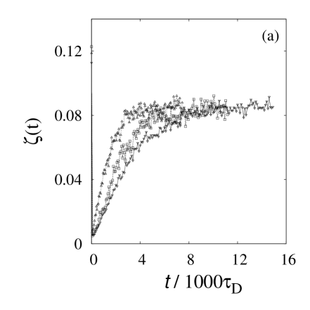
7.8 Thermodynamic equilibrium
After the crossover time , during which plasma remains trapped in an out of equilibrium qSS, it should relax to the thermodynamic equilibrium in which the particle density and velocity distributions should be given by the usual Boltzmann-Gibbs statistical mechanics
| (163) |
and
| (164) |
where is the normalization constant, is the Lagrange multiplier for conservation of energy, and is the potential of mean force [97]. For large number of particles, the correlations become unimportant and . The potential must then satisfy the Poisson-Boltzmann equation,
| (165) |
with the boundary conditions and . The solution to this equation can be obtained numerically. In Fig 32 we compare the predictions of the Boltzmann-Gibbs statistical mechanics with the results of MD simulations. The computer runs were performed with not too many particles to allow the system to relax to equilibrium within reasonable CPU time. Fig 32 shows the marginal distributions , and with and given by Eqs (163) and (164). As expected, after a sufficiently long time the system relaxes to the thermodynamic equilibrium.

8 The Hamiltonian Mean Field model
The gravitational and plasma systems studied up to now are of great practical importance. From the perspective of statistical mechanics, however, they have a serious drawback — they do not exhibit a phase transition. In the last two sections of this review we will consider two systems with long-range forces which do show a spontaneous symmetry breaking. In particular, we are interested to explore how the phase transitions between the qSSs differ from the usual equilibrium phase transitions.
The first system that we will study is the Hamiltonian Mean Field (HMF) model. The HMF is a mean-field version of the -model, in which all spins interact with each other [190, 191]. It has become a paradigm of a system with long-range interaction [192, 193, 194, 195], and is especially interesting due to its phase transition. For one-dimensional systems with short-range forces the Mermin-Wagner theorem prohibits spontaneous symmetry breaking in 1D [196]. The phase transition in the HMF is only possible because of the infinite range interaction between the spins [197, 198]. The HMF model can also be considered a simplified representation of a one-dimensional self-gravitating [199] or Coulomb system [200] on a ring, and has some similarity with the Colson-Bonifacio model of a single-pass free electron laser [201, 202, 203, 204].
8.1 The model
The HMF model can be interpreted in terms of interacting spins or as particles confined to move on a circle of radius one. The particle interpretation is more convenient for studying the dynamics of this model, so we will adopt it for most of our discussion. The dynamics of particles of the HMF is governed by the Hamiltonian [191]
| (166) |
where is the coordinate and the conjugate momentum of the -th particle, and is a parameter that controls the intensity of the interaction. The sign of determines the type of coupling between the particles: if , the interaction is attractive and the coupling is ferromagnetic; if , the interaction is repulsive and the coupling is antiferromagnetic.
The Hamiltonian (166) is a simplification of a one-dimensional gravitational or a Coulomb system with periodic boundary conditions and a neutralizing background. For example, consider a system formed by particles distributed along a ring of unit radius, i.e. with position . The Poisson equation is
| (167) |
where depends on the system under consideration, and , if . In the gravitational case , where is the gravitational constant, is the particle mass and the total mass. For the Coulomb case, , where is the charge density, the total charge and the vacuum permittivity. The term represents the uniform neutralizing background which is necessary both for Coulomb and gravitational systems with periodic boundary conditions.
Expressing the Dirac delta in its Fourier representation, and integrating the Poisson equation, the potential produced by particles is found to be
| (168) |
The potential is normalized so that when . Truncating the series at and taking , we recover the potential of the HMF model.
We will consider the ferromagnetic HMF model. Rescaling time, we can set . The Hamiltonian (166) can then be written as
| (169) |
or
| (170) |
The order parameter of the system is the magnetization per particle, , which measures how “bunched” is the particle distribution. If the particles are uniformly distributed over the ring. The components of the magnetization are
| (171) |
and
| (172) |
The energy per particle, , can be written as
| (173) |
and the one particle energy is
| (174) |
If the initial distribution is symmetric in , then , and in the thermodynamic limit, it will remain so throughout the evolution [25]. For now we will only consider symmetric distributions and set .
8.2 Thermodynamic equilibrium
Classical statistical mechanics provides a prediction for the thermodynamic equilibrium of the HMF model [191]. In this subsection, we shall briefly describe the results in the microcanonical ensemble. A more extensive treatment of the equilibrium state of the HMF model can be found in ref. [7].
The microcanonical ensemble is defined by the surface of constant energy in the -dimensional configuration space, being the number of degrees of freedom of each particle ( for the HMF),
| (175) |
where and are -dimensional vectors representing the positions and velocities of all particles that compose the system: and . Thus, we also write and .
The Boltzmann entropy per particle is which is calculated to be [205, 7]
| (176) |
where is the modified Bessel function of the first kind. The curve is shown on Fig 33. The equilibrium magnetization is obtained by solving the equation
| (177) |
and is plotted as a function of in Fig 34. Finally, Fig 35 shows the inverse temperature as a function of . These figures indicate a second-order phase transition between ferromagnetic and paramagnetic states at .


8.3 Out of equilibrium, quasistationary states
The results shown in subsection 8.2 are valid if the HMF is able to relax to thermodynamic equilibrium. However, as we have seen throughout this report, in thermodynamic limit systems with long-range interactions do not reach the equilibrium, but become trapped in a qSS, the lifetime of which diverges with the number of particles [98]. Thus, in practice the equilibrium state will never be achieved by the HMF model with a large enough number of particles. To explore the properties of the qSS and the possible phase transitions between the different nonequilibrium states, we use MD simulations. In this report we focus on simulations with initial distributions of the one-level waterbag type — Eq (178); for results of studies of the qSSs of the HMF model using other types of initial distributions, see for example Refs. [206, 207, 208].
At the particles are distributed in accordance with the one-level waterbag distribution,
| (178) |
where is the Heaviside step function. The constants (density), (maximum value of ) and (maximum value of ) are determined by the normalization of the distribution, initial magnetization () and mean energy (), respectively,
| (179) | ||||
| (180) |
and
| (181) |
These lead to
| (182) | |||
| (183) |
and
| (184) |
To simulate a system composed of particles, we use two vectors of dimension , where the -th component of the first vector represents the angle of the -th particle, and similarly the -th component of the second vector is the momentum of the respective particle. As the initial condition, each and take a random value between and , respectively. For each of these particles, we consider that there exists a particle in a symmetrical position in phase space: and , which ensures that and increases the simulation speed — since the dynamics is symmetric, we only need to integrate the motion of half of the particles.
The trajectory of each particle is governed by the equation of motion , or
| (185) |
The numerical integration is implemented using a fourth-order symplectic integrator [209], available online from E. Hairer [210]. To control the numerical precision, the error in conservation of energy per particle , given by equation (173), was kept at approximately .
Figure 36 shows examples of two initial phase space distributions, panels (a) and (c), and the respective distributions after a qSS have been achieved, panels (b) and (d). The simulations were performed with particles. The initial magnetization was the same in both simulations, — both initial waterbags had the same . The ’s for the two distributions were different corresponding to energies (a) and (c) . The two initial conditions lead to different phases: the higher energy configuration leads to a paramagnetic (homogeneous) distribution, panel (b), while the system with lower energy remains magnetized, panel (d).
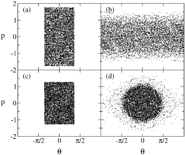
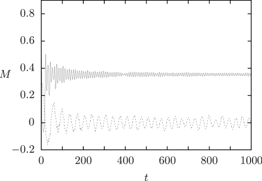
The final qSS state depends both on the initial magnetization and energy . This is very different from the state of thermodynamic equilibrium which depends only on . The evolution of for two systems with the same energy and different values of is shown in Fig 37. A system with an initial magnetization quickly relaxes to a paramagnetic state in which its magnetization oscillates around . On the other hand, a system with remains magnetized. In both cases, the magnetization oscillates around its quasi-stationary value , given by the temporal average of [206]. However, while the oscillations inside the ferromagnetic state are clearly damped, the amplitude of oscillations in the paramagnetic state remains finite. The difference between the two states is that inside the ferromagnetic phase the particles experience a finite mean-field potential produced by while in the paramagnetic phase the average potential is zero. This means that inside the ferromagnetic state some particles can enter in resonance with the oscillations of the potential and gain energy from the collective motion. This, in turn, will result in Landau damping of the magnetization and the relaxation to qSS. In the paramagnetic phase, oscillates around zero, so there is no resonant mechanism to dampen the oscillations.
The location of the phase transition can be determined by performing simulations for different initial conditions, varying for a fixed initial magnetization and calculating . The resulting nonequilibrium phase diagram for the HMF model is shown in Fig 38. The results are fairly similar to the nonequilibrium phase diagram found using the Lynden-Bell entropy [211], yet has some differences, primarily as to the order of the phase transition in some regions, as will be seen further on in this chapter, and in the location of the transition for higher initial magnetizations.
It is interesting to compare the nonequilibrium phase diagram with the one found for the equilibrium of the HMF model. In equilibrium, the critical energy separates the paramagnetic () from the ferromagnetic phase () and is independent of the initial magnetization, as is shown by the dashed-dotted line of zero slope in the phase diagram, Fig 38. On the other hand, the transition between the nonequilibrium ferromagnetic and paramagnetic phases occurs at different values of , depending on the initial magnetization. This transition is represented by a solid line. The shaded region is the forbidden zone — since the minimum kinetic energy is zero, determines the minimum allowed energy per particle . The diagram also shows a region in which the nonequilibrium order-disorder transition is not well defined: the wide, shaded line around the critical line for , approximately. For these values of , there are regions where the average energy is above the critical line, yet in which the system remains magnetized. Similar regions, or reentrances, have also been observed in studies of the HMF model using numerical resolution of the Vlasov equation [212] and Lynden-Bell statistics [213]. Finally, while the equilibrium phase transition between the ferromagnetic and paramagnetic phases is of second order [7], the nonequilibrium phase transition is of first order.
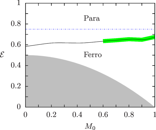
In our studies of self-gravitating systems and plasmas, we saw the importance of the virial theorem to determine when strong collective oscillations will occur. However, since the potential of the HMF is not a homogeneous function of the separation between the particles, we can not directly apply the results of Section 4.4 to determine the virial condition. To discover under what conditions the magnetization of the HMF model will remain constant, so that the parametric resonances will not be excited, we need to derive a Generalized Virial Condition (GVC).
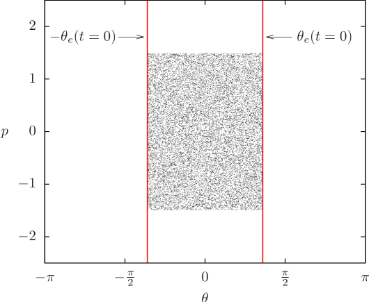
To do this we define the envelope of the particle distribution of the HMF as [19]
| (186) |
Note that at , the envelope coincides with the maximum of the initial waterbag distribution, , see Fig 39. Differentiating equation (186) twice with respect to time, we find
| (187) |
As the result of the conservation of energy, see equation (173), in the first term, the mean square velocity is . To calculate the other averages, we assume the marginal distribution in remains uniform in the interval and zero outside. Using this approximation, the second term of equation (187) reduces to
The last term of equation (187) may be neglected by disregarding the correlations between and . The resulting envelope equation is
| (188) |
where we have used
| (189) |
Fig 40 compares the evolution of magnetization , predicted by the equations (188) and (8.3), with the magnetization obtained using the full -body MD simulation. We see an excellent agreement between the theory and simulation, especially at short times. For longer times, the amplitude of the magnetization observed in the simulations is damped, while the envelope oscillations do not. This occurs because the envelope equation is conservative, while in the simulation the parametric resonances transfer the energy from the collective oscillations to the individual particles.
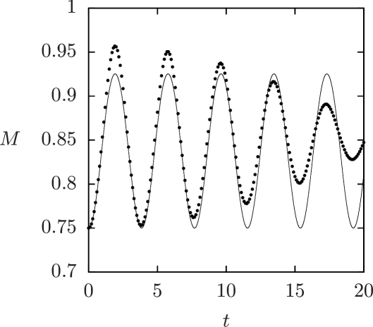
The GVC corresponds to the initial condition for which the envelope does not oscillate, so that . This happens when [19],
| (190) |
so that . Eq. (190) defines the GVC condition which is plotted by the dashed line in the nonequilibrium phase diagram of Fig 41.
To test the GVC we perform MD simulations starting with initial waterbag distributions which lie directly on top of the GVC curve (190). We then plot with triangles in Fig 41 the final magnetization to which the system relaxes (note that for both the initial and the final state the energy is the same). We see that the final stationary magnetizations are almost exactly the same as the initial magnetizations . Furthermore, for systems with initial conditions off the GVC curve, the magnetization quickly changes and begins to oscillate around the stationary value corresponding to on the GVC curve with the same . For example, points and of Fig 41 each represent initial conditions off the GVC. Let us call the coordinates of these points and , respectively. The stationary values obtained using the MD simulations correspond to and . The arrows next to points and indicate the values of and on the GVC curve to which the system relaxes. This result is quite surprising, since the distribution functions for the initial and the final state are very different for systems that do not satisfy the GVC [19]. It is not clear at this moment why the approximate GVC derived using the waterbag distribution works so well to predict the final magnetizations for systems which initially are very far from their qSS.
Eq. (190) has an unstable branch, represented by the blue dotted line in Fig 41. If the initial conditions place the system exactly on this branch, the magnetization will remain the same, however, any perturbation will make the system evolve from the line of unstable fixed points toward the line of stable ones, represented by the red dashed curve.
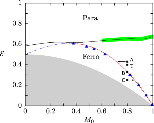
8.4 Lynden-Bell theory for the HMF model
The LB theory has been extensively applied to the HMF model, in some cases showing reasonable agreement with the results of MD simulations [54, 214, 55, 215]. From the examples of gravity and plasma, however, we expect that LB theory should only work when the initial distribution satisfies the GVC. For non-virial initial conditions, resonances should drive the HMF into a qSS with a core-halo particle distribution [25, 19].
The LB distribution for the HMF model is given by [55]
| (191) |
where . The phase space density is determined by the initial distribution (182), while and are the Lagrange multipliers used to preserve the norm and the energy. Solving the system of equations
| (192) | ||||
| (193) |
and
| (194) |
we can calculate , and and obtain the particle distribution predicted by LB for the qSS.
In Fig 42, we show the marginal distributions, in angle and momentum, obtained using MD simulations, and compare them with the predictions of LB theory. Three different initial conditions are shown in Fig 41: panels and correspond to non-virial initial conditions, while panel shows the initial condition that lies on the GVC. For the non-virial initial conditions, the distribution functions show a significant deviation from the LB theory. On the other hand, the initial distribution that satisfies the GVC is found to relax to the qSS which is well described by LB theory, panel of Fig.41.
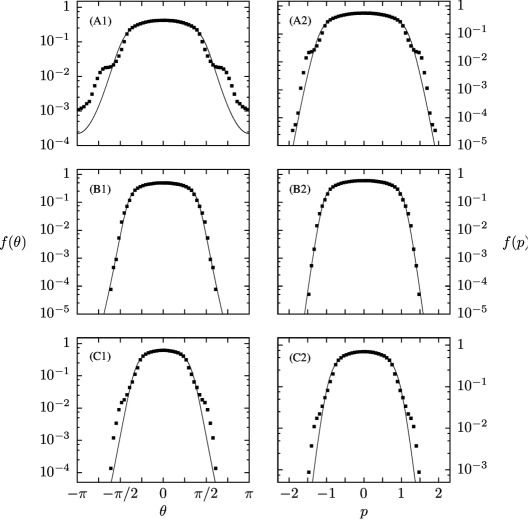
8.5 The test particle model
The discrepancies between the results of MD simulations and the LB theory, for initial distributions which do not satisfy the GVC, are a consequence of the parametric resonances which transfer the energy from the collective motion to the individual particles [19]. To study these resonances we, once again, appeal to the test particle model.
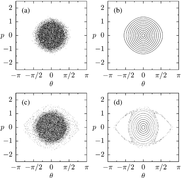
The test particles obey the equation of motion (8.3), with the magnetization determined by the envelope equation, . Fig 43 shows the Poincaré sections of test particle dynamics — the phase space of the test particles plotted when is at its minimum — compared with the phase space of the HMF, obtained using MD simulation. Two cases are shown: top panels correspond to the initial conditions that obey the GVC (point of Fig 41), while the bottom panels correspond to the initial conditions slightly off the GVC (point of Fig 41). For the initial distribution satisfying the GVC, the test particle dynamics is regular and no halo is formed. On the other hand, for the non-virial initial distributions (off the GVC), we see resonances which lead to the halo formation in the HMF.
The mechanism of core-halo formation in the HMF is the same as was discussed for gravitational and plasma systems. The parametric resonances transfer the energy from the collective motion to the individual particles. This, in turn, dampens the collective oscillations, forcing the core particles into low energy orbits. Once the oscillations die out completely, the dynamics of all the particles becomes integrable, and the ergodicity is irreversibly broken. The high energy particles become trapped inside a halo, while the low energy particles form a degenerate core. The LB theory, which relies on the assumptions of ergodicity and efficient mixing [100], is not able to describe such qSSs [19].
8.6 The core-halo distribution
The core-halo distribution for the HMF model is [25]
| (195) |
with the one-particle energy given by . To calculate this distribution we need to determine , , and . The parameters and are calculated using the conservation of energy and norm, respectively,
| (196) |
| (197) |
and is given by
| (198) |
To calculate for gravitational systems and plasmas we have used the test particle dynamics to locate precisely the resonant orbit. However, there is an inherent difficulty in using this approach for the HMF model. The interaction potential for HMF particles is bounded from above. Depending on the initial conditions, some particles can gain enough energy to completely escape the confining potential, and start moving in rotating orbits. This makes it difficult to pinpoint the highest possible energy of the resonant particle. In this sense, the HMF model is similar to 3d self-gravitating systems, for which particles can escape the gravitational potential of the cluster. Another difficulty with the test particle dynamics is that while the system is spatially periodic, the envelope equation (188) is not. The oscillations of the envelope may be so large that the envelope surpasses , in which case an artificial periodicity must be introduced into the test particle dynamics. In spite of these difficulties, we can still attempt to use the core-halo distribution with the approximate values of to locate the order-disorder transition in this model. Figure 44 shows the qSS magnetization as determined by the core-halo theory and the test particle dynamics for various values of at fixed initial magnetization . The core-halo theory predicts a first order phase transition between the paramagnetic and ferromagnetic phases. In the same figure we also plot the prediction of LB theory. Although the distribution functions of LB theory deviate significantly from the results of MD simulations in the tails, far from the transition point the theory accounts quite accurately for the values of . LB theory, however, incorrectly predicts that the phase transition between the qSSs for is of second order [211], while the simulations find it to be of first order, Fig 44. Numerical resolution of the Vlasov equation, which may be used to study the dynamics of the HMF model [216], also shows only first-order transitions in the HMF [212] .
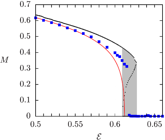
At the moment, we lack a general method to calculate the halo energy for arbitrary values of and . The envelope equation and the test particles dynamics allow us to make accurate predictions of for distributions close to the GVC. To predict the final particle distributions in the qSS which are far from the GVC, we can use a short MD simulation of the full HMF model with not too many particles. Since the formation of resonances is a fast process, the can be defined as the highest energy achieved by any particle after a few oscillations of . Fig 45 shows that this procedure leads to an excellent description of the final qSS.
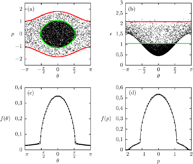
8.7 Relaxation to equilibrium
For finite , the lifespan of the qSS is finite, and eventually a crossover to thermodynamic equilibrium occurs [217]. In equilibrium the particle distribution has the usual Maxwell-Boltzmann form, with the magnetization given by the solution of equation (177) [7]. The relaxation to equilibrium is shown in Fig 46, which demonstrates the evolution of for different values of . The initial condition ( and ) is such that the qSS is paramagnetic, while the equilibrium state is ferromagnetic. For this energy, the equilibrium magnetization is , represented by the black dotted line in Fig 46. As the figure shows, the fewer particles in the system, the faster the magnetization relaxes to the equilibrium value. Rescaling time with , with , all the curves collapse onto one universal curve. The lifespan of the qSS therefore scales with . The exponent is the same as the value found in other studies of the HMF model [98]. However, recent large-scale MD simulations show that for large , the exponent crosses over to . This is consistent with the arguments based on the Balescu-Lenard equation, which suggest that the crossover time from a paramagnetic (homogeneous) qSS to a ferromagnetic equilibrium state should scale as [218, 219, 220].

9 The Generalized Hamiltonian Mean Field model
From the perspective of statistical mechanics, the HMF model is significantly richer than self-gravitating or plasma systems. Unlike these systems, the HMF possesses a genuine nonequilibrium phase transition between qSSs. The structure of the phase diagram of the HMF, however, is still relatively simple, since only paramagnetic and ferromagnetic phases exist. To explore further the differences between equilibrium and nonequilibrium phase transitions, we introduce a Generalized Hamiltonian Mean Field (GHMF) model. In addition to paramagnetic and ferromagnetic phases, this model also has a nematic phase. In this section we will compare the equilibrium and nonequilibrium phase diagrams of the GHMF and show that in the new qSS nematic phase, particles are once again distributed in accordance with the core-halo distribution.
9.1 The model
The Hamiltonian of the GHMF model is given by
| (199) |
where and [221]. This model is a long-range version of the models studied in references [222, 223]. Considering the particles as a collection of spins, the generalized nematic coupling favors either alignment or misalignment of spins. For example, for , it favors either parallel or antiparallel spins. From the perspective of the particle dynamics, either homogeneous or bunched states are possible, with the number of bunches controlled by the parameter .
The order parameters for the GHMF model are the generalized magnetizations
| (200) |
and
| (201) |
Note that the full definition of the magnetizations should include and , analogous to the HMF model; however, we neglect these terms because only initial distributions symmetric in will be considered.
The GHMF Hamiltonian (199) can be rewritten as
The average energy per particle is
| (202) |
and the one-particle energy is
| (203) |
9.2 Thermodynamic equilibrium
The procedure for obtaining the equilibrium values of and is the same as used for the HMF model. Here we present only the final results; more details can be found in the reference [221]. The microcanonical entropy is given by
| (204) |
The equilibrium magnetizations correspond to the maximum of the entropy (9.2) and must satisfy the coupled equations
| (205) |
and
| (206) |
where
| (207) |
| (208) |
The roots of equations (205), (206), (207) and (208) determine the equilibrium magnetizations for a given , and .

Figure 47 shows the phase diagram for [221]. Most transitions are of second order (dashed lines), except for a small region near , where the transition is of first order (solid line). The equilibrium distribution functions for the three phases are illustrated in the right-hand panels of Fig 47 :
-
(a)
the paramagnetic phase (),
-
(b)
the nematic phase () and
-
(c)
the ferromagnetic phase ().
The generalized magnetizations (solid line) and (dotted line) as a function of energy, for four values of , are shown in Fig 48: panels (a), (b) and (c) show second order transitions (nematic-paramagnetic, ferromagnetic-paramagnetic, and ferromagnetic-nematic, respectively), and panel (d) shows a first order ferromagnetic-paramagnetic transition. In the latter case, the critical energy is the energy for which the entropies of the ferromagnetic and paramagnetic phases are equal.

9.3 Nonequilibrium quasi-stationary states
Unlike the equilibrium states of the GHMF, which only depends on the initial energy, the qSSs depend explicitly on the initial particle distribution. In this Report we will explore how the ordered ferromagnetic and nematic phases arise from the initially homogeneous particle distribution of the waterbag form,
| (209) |
In MD simulations, particles are distributed so that , where is the position and momentum of the -th particle. The average energy per particle is . The equation of motion for the -th particle is given by
| (210) |
In simulations we observe that the system quickly relaxes into a qSS in which and oscillate slightly around their average values ( and ), which depend on and . Phase transitions are located by performing a series of simulations varying , for a given value of , and calculating the average value of and over a time interval during the QSS. The transitions are found to be of first order.
9.4 Stability of the homogeneous state
The distribution given by Eq (209) is a stationary solution of the Vlasov equation. Therefore, a transition between a homogeneous state and a non-homogeneous state, either ferromagnetic or nematic, can occur only as a result of a dynamical instability. Therefore, by studying the stability of the homogeneous solution, we should be able to gain an insight into the structure of the phase diagram of the GHMF model. A similar approach has also been used to study the HMF model in an external magnetic field [224] and was shown to agree with the predictions of the linear response theory [225].
To explore the stability of the distribution function Eq. (209), we perturb the upper momentum limit, , as
| (211) |
We define the generalized magnetizations as
| (212) |
where . Differentiating the term twice with respect to time, we find the equation of motion
| (213) |
The average values are calculated using the distribution function . Thus, the integral above involves an infinite series of cosines. For our analysis, we consider the series up to , which will prove to be sufficient to locate and determine the order of the phase transitions. Performing the averages, we obtain a system of differential equations for the generalized magnetizations,
| (214) | |||
| (215) | |||
| (216) | |||
| (217) |
where
| (218) | ||||
| (219) | ||||
| (220) |
and
| (221) |
Equations (214)–(217) have been written so as to separate linear terms on the left hand side and the nonlinear terms on the right hand side of the equality. To calculate the paramagnetic-ferromagnetic and paramagnetic-nematic phase boundaries, we analyze the linear stability of and . Neglecting the nonlinear terms (218)–(221), equations (214) and (215) take the form , whose solutions are . Thus, the magnetizations will remain stable only if . If , the exponents will become real and any infinitesimal fluctuation will experience an exponential growth, destabilizing the paramagnetic phase. The phase boundary that separates the paramagnetic phase from the ferromagnetic and nematic phases is, therefore, determined by the conditions and , respectively. According to the equations (214) and (215), and and we find the phase boundaries to be
| (222) |
and
| (223) |
where and are the boundaries for the paramagnetic-ferromagnetic and paramagnetic-nematic transitions, respectively.
To determine the order of the phase transitions, we study the fixed points of the system of equations (214)–(217), including the nonlinear terms (218)-(221). Although the equations are conservative, we expect that in the full GHMF, the Landau damping will provide dissipation which will drive the system towards the qSS. The dissipation can be included by adding terms proportional to into Eqs. (214)–(217). This will make the system relax to the stable fixed points of equations (214)–(217), which will then correspond to the generalized magnetizations in the final qSS. We find that once the paramagnetic-nematic boundary is crossed, the value of jumps discontinuously from zero to approximately , while remains zero. The jump in is very close to the value observed in MD simulation, , independent of . For the paramagnetic-ferromagnetic transition, the two magnetizations jump from zero to finite values which depend on . In this case the theory is again consistent with the simulations predicting that when crossing the phase transition boundary, is always negative, while may be positive or negative.
The ferromagnetic-nematic phase boundary should be determined by the two growth rates () of and . If grows faster than , the system will reach the ferromagnetic fixed point prior to reaching the nematic one, and vice versa. Therefore, we expect that the ferromagnetic-nematic phase boundary should be close to the curve ,
| (224) |
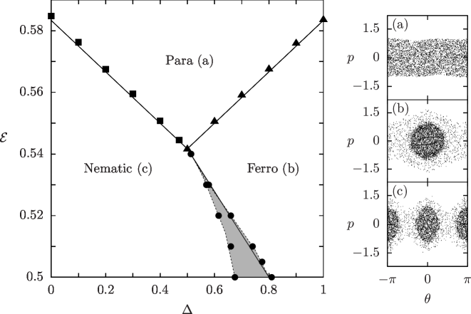
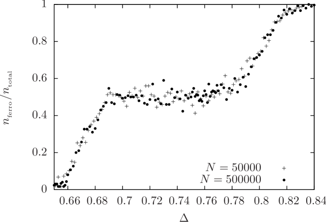
Figure 49 show the nonequilibrium phase diagram for the GHMF model for an initially homogeneous particle distribution. The theoretically calculated phase boundaries obtained using equations (222), (223) and (224) are shown as the solid lines. The results of MD simulations are shown as symbols. The paramagnetic-nematic and the paramagnetic-ferromagnetic phase boundaries predicted by the theory are in perfect agreement with the results of MD simulations. For the ferromagnetic-nematic transition the simulations find an instability region in which either phase can occur with equal probability, Fig. 50. The theoretically predicted phase boundary for the ferromagnetic-nematic transition Eq. (224) passes through the instability region.
9.5 The core-halo distribution
The particle distributions in the ferromagnetic and nematic phases are, once again, of the core-halo form, Eq. (195), with the one-particle energy given by Eq. (203). In Fig. 51 we plot a snapshot of the phase space of the GHMF and the energy of each particle once the system has relaxed into a nematic qSS. In both panels of Fig. 51 a core-halo structure can be clearly seen. In the nematic phase it actually appears that there are two cores. This happens because and the one-particle energy has two minimums at and . Both cores, however, appear in the core-halo distribution function, given by
| (225) |
where and are the phase space densities of the core and halo, respectively; and are the maximum energies of the core and halo, respectively; and the one-particle energy is given by Eq (203).
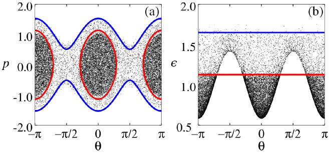
In Fig. 52 we plot the marginal distributions calculated using the core-halo theory,
| (226) |
and
| (227) |
with given by Eq (225), and compare them with the results of MD simulations. The halo energy (blue line in Fig 51(b)) was obtained using a short simulation with particles, which ran for only dynamical times. The Fermi energy and the halo phase space density were calculated using the conservation of energy and of norm. The predicted value for the Fermi energy is the red line in Fig. 51(b). In panel (a) of the same figure we show the orbit of a particle with energy equal to (red line). This orbit perfectly encloses the core. In the same panel, the blue line represents an orbit of a particle with energy .

As with other long-range systems, eventually the GHMF will relax to thermodynamic equilibrium described by the Boltzmann-Gibbs statistical mechanics. The resultant phase diagram will then change to the one shown in Fig 47. In the thermodynamic limit , this relaxation, however, will never occur and the system will remain trapped forever in one of the qSSs.
10 Conclusions and Perspectives
In this Review we have explored statistical mechanics of systems with long-range interactions. A number of different examples have been considered, ranging from plasmas and self-gravitating systems to the kinetic spin models. In the thermodynamic limit, these systems do not relax to the Boltzmann-Gibbs equilibrium, but become trapped in the qSSs, the life time of which diverges with the number of particles . If is small, after staying in the qSS for a time of approximately , where is usually larger or equal to one, a system relaxes to the thermodynamic equilibrium described by the usual Boltzmann-Gibbs statistical mechanics. This is what has been observed for all the models studied so far — after a time , they all (with the exception of 3D gravity, which always remains out of equilibrium) relaxed to thermodynamic equilibrium. In this respect, speculations that long-ranged systems should be described by the non-extensive Tsallis statistics are unfounded [226].
In the case of plasmas and elliptical galaxies, the number of “particles” is so large that the state of thermodynamic equilibrium can not be reached within the life time of the universe. Furthermore, for 3D gravity, we saw that there is an additional problem related to the bounded (from above) nature of Newton’s gravitational potential and the resulting flux of evaporating particles. For 1D and 2D gravitational systems, on the other hand, there is no problem with particle evaporation. After a short time, these systems relax to qSSs which have a characteristic core-halo structure. The distribution function that describes qSSs of self-gravitating systems is the same as the one that describes the qSS of magnetically confined plasmas and of spin systems. The ubiquity of core-halo distributions, observed in so many different contexts, suggests that there is a significant degree of universality to the process of collisionless relaxation. The core-halo distribution appears to be a universal attractor — in a coarse-grained sense — analogous to the Maxwell-Boltzmann distribution for systems with short-range forces.
A qSS reached by a long-range interacting system depends explicitly on the initial particle distribution. In this Report we have considered only the initial conditions of the waterbag form. In the future, it will be important to extend the theory to more complex initial conditions. Preliminary work in this direction indicates that multilevel distributions lead to significantly more complex qSSs, with very interesting topological structure which, nevertheless, preserves some of the core-halo characteristics [207]. Curiously, for such initial distributions, the LB theory fails to describe the qSSs, even when initial conditions satisfy the virial theorem. This indicates that for multilevel distributions mixing is even poorer than it is for one level waterbags. Furthermore, even for one-level waterbag distributions satisfying the virial condition, there are small deviations between the results of simulations and the LB theory, and some halo formation may be observed. This suggests that that the core-halo distribution may also be relevant for predicting the qSS of initially virialized waterbag distributions. Since for the parametric resonances are not be excited, the halo energy in this case should be the same as the energy of the most energetic particle of the initial distribution. In Fig 53 we compare the predictions of the core-halo and the LB theories with the results of MD simulations for 1D self-gravitating system with . It appears that even in this case the core-halo theory agrees better with the results of simulations than does the LB approach. This suggests that mixing and ergodicity are not perfect even for initially virialized distributions. This, however, should be tested for other models discussed in this Review.
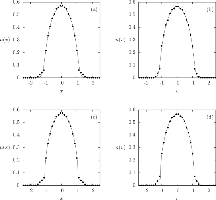
A trapping of a system in a qSS is a consequence of the ergodicity breaking. The process of Landau damping decreases the amplitude of collective oscillations which are responsible for the energy transfer between the particles. For long-range systems, there are no collisions (correlations) between the particles, and the only mechanism of energy transfer is the wave-particle interaction. Therefore, once the oscillations have completely died out, each particles will move in a static mean-field potential and the ergodity of the system will be broken. All the systems that have been considered so far had either spherical (in 3D) or polar (in 2D) symmetry. The equations of motion for a particle inside such potentials are integrable. This, in general, is not true for asymmetric potentials for which particle trajectories can become chaotic. It should be of great interest to explore if the chaotic dynamics in the qSS can lead to a faster relaxation to the Boltzmann-Gibbs equilibrium and a shorter lifetime of a qSS.
There are a number of outstanding open question which remain to be addressed. Can the core-halo theory developed above be extended to study 3D self-gravitating systems? For such systems the halo will extend all the way to infinity. At the moment we do not have an understanding of the structure of such halos. Furthermore, both 2D and 3D gravitational systems are susceptible to symmetry breaking instabilities [227]. The simulation methods used in the present work, which primarily relied on the Gauss’s law, do not allow us to study such instabilities. The theoretical understanding of the symmetry breaking mechanism that leads to asymmetric QSS is still lacking and it is not clear how to extend the core-halo theory to describe the asymmetric stationary states. Finally, in the future it will be important to move beyond the waterbag initial distributions. As discussed above, multilevel initial distributions appear to exhibit ergodicity breaking and poor mixing even when they are virialized. This makes the study of such initial conditions very challenging [207]. Nevertheless, it has been observed that even such complex initial distributions also relax to core-halo QSS, with the particle distribution in the core well fitted by polytropic distributions [208].
In spite of their ubiquity, long-range interacting systems are still poorly understood. They are the unexplored frontier of statistical physics. We hope that the present Review helps to attract attention of the statistical mechanics community to this fascinating field.
Y.L. would like to thank Michael Fisher, without whose insistence and encouragement this review would not have been written. This work was partially supported by the CNPq, FAPERGS, INCT-FCx, and by the US-AFOSR under the grant FA9550-12-1-0438.
References
- [1] M. J. Klein, Thermodynamics in Einstein’s Thought, Science 157 (3788) (1967) 509. doi:10.1126/science.157.3788.509.
- [2] M. E. Fisher, The free energy of a macroscopic system, Archive for Rational Mechanics and Analysis 17 (5) (1964) 377.
- [3] D. Ruelle, Superstable interactions in classical statistical mechanics, Communications in Mathematical Physics 18 (2) (1970) 127.
-
[4]
M. Kac, On the Partition
Function of a One-Dimensional Gas, Physics of Fluids 2 (1) (1959)
8–12.
URL http://link.aip.org/link/?PFLDAS/2/8/1 - [5] M. Kac, G. E. Uhlenbeck, P. C. Hemmer, On the van der Waals Theory of the Vapor-Liquid Equilibrium. I. Discussion of a One-Dimensional Model, Journal of Mathematical Physics 4 (2) (1963) 216. doi:10.1063/1.1703946.
- [6] G. A. Baker, Ising Model with a Long-Range Interaction in the Presence of Residual Short-Range Interactions, Physical Review 130 (4) (1963) 1406. doi:10.1103/PhysRev.130.1406.
- [7] A. Campa, T. Dauxois, S. Ruffo, Statistical mechanics and dynamics of solvable models with long-range interactions, Physics Reports 480 (3-6) (2009) 57–159. doi:10.1016/j.physrep.2009.07.001.
- [8] J. Barré, D. Mukamel, S. Ruffo, Inequivalence of Ensembles in a System with Long-Range Interactions, Physical Review Letters 87 (3) (2001) 30601. doi:10.1103/PhysRevLett.87.030601.
- [9] W. Thirring, Systems with Negative Specific Heat, Zeitschrift für Physik 235 (4) (1970) 339.
- [10] D. Lynden-Bell, R. M. Lynden-Bell, On the negative specific heat paradox, Monthly Notices of the Royal Astronomical Society 181 (1977) 405.
- [11] A. El-Zant, Approach to equilibrium in N-body gravitational systems, Physical Review E 58 (4) (1998) 4152. doi:10.1103/PhysRevE.58.4152.
- [12] D. Lynden-Bell, Negative specific heat in astronomy, physics and chemistry, Physica A: Statistical Mechanics and its Applications 263 (1999) 293. doi:10.1016/S0378-4371(98)00518-4.
-
[13]
M. Kiessling, T. Neukirch,
Negative specific heat
of a magnetically self-confined plasma torus, Proceedings of the
National Academy of Sciences of the United States of America
100 (4) (2003) 1510.
URL http://www.pnas.org/content/100/4/1510.short - [14] W. Thirring, H. Narnhofer, H. Posch, Negative Specific Heat, the Thermodynamic Limit, and Ergodicity, Physical Review Letters 91 (13) (2003) 130601. doi:10.1103/PhysRevLett.91.130601.
- [15] L. Reichl, A Modern Course In Statistical Physics, 2nd Edition, Wiley-Interscience, 1998.
- [16] T. Tsuchiya, T. Konishi, N. Gouda, Quasiequilibria in one-dimensional self-gravitating many-body systems, Physical Review E 50 (4) (1994) 2607. doi:10.1103/PhysRevE.50.2607.
- [17] F. Borgonovi, G. L. Celardo, M. Maianti, E. Pedersoli, Broken Ergodicity in Classically Chaotic Spin Systems, Journal of Statistical Physics 116 (5–6) (2004) 1435. doi:10.1023/B:JOSS.0000041745.62340.00.
- [18] P. Chen, M. Cross, Mixing and thermal equilibrium in the dynamical relaxation of a vortex ring, Physical Review Letters 77 (20) (1996) 4174–4177. doi:10.1103/PhysRevLett.77.4174.
- [19] F. P. da C. Benetti, T. N. Teles, R. Pakter, Y. Levin, Ergodicity Breaking and Parametric Resonances in Systems with Long-Range Interactions, Physical Review Letters 108 (2012) 140601. doi:10.1103/PhysRevLett.108.140601.
- [20] W. Braun, K. Hepp, The Vlasov dynamics and its fluctuations in the 1/N limit of interacting classical particles, Communications in Mathematical Physics 56 (2) (1977) 101–113. doi:10.1007/BF01611497.
- [21] A. Gabrielli, M. Joyce, Gravitational force in an infinite one-dimensional Poisson distribution, Physical Review E 81 (2) (2010) 1–9. doi:10.1103/PhysRevE.81.021102.
- [22] M. Luwel, G. Severne, P. Rousseeuw, Numerical study of the relaxation of one-dimensional gravitational systems, Astrophysics and Space Science 100 (1–2) (1984) 261. doi:10.1007/BF00651601.
- [23] Y. Levin, R. Pakter, T. Teles, Collisionless Relaxation in Non-Neutral Plasmas, Physical Review Letters 100 (4) (2008) 040604. doi:10.1103/PhysRevLett.100.040604.
- [24] T. N. Teles, R. Pakter, Y. Levin, Relaxation and emittance growth of a thermal charged-particle beam, Applied Physics Letters 95 (17) (2009) 173501. doi:10.1063/1.3254245.
- [25] R. Pakter, Y. Levin, Core-Halo Distribution in the Hamiltonian Mean-Field Model, Physical Review Letters 106 (2011) 200603. doi:10.1103/PhysRevLett.106.200603.
-
[26]
M. Hénon,
L’évolution
initiale d’un amas sphérique, Annales d’Astrophysique 27 (1964) 83.
URL http://adsabs.harvard.edu/full/1964AnAp...27...83H - [27] A. M. Salzberg, Exact statistical thermodynamics of gravitational interactions in one and two dimensions, Journal of Mathematical Physics 6 (1) (1965) 158. doi:10.1063/1.1704254.
-
[28]
M. Lecar, A
one-dimensional self-gravitating stellar gas, in: G. I. Kontopoulos (Ed.),
The Theory of Orbits in the Solar System and in Stellar
Systems. Proceedings from Symposium no. 25 held in Thessaloniki,
1964., International Astronomical Union, Academic Press, 1966, p. 46.
URL http://adsabs.harvard.edu/full/1966IAUS...25...46L -
[29]
F. Hohl, J. W. Campbell,
Statistical
Mechanics of a Collisionless Self-Gravitating System, The Astronomical
Journal 73 (7) (1968) 611.
URL http://adsabs.harvard.edu/full/1968AJ.....73..611H - [30] R. H. Miller, Numerical experiments in collisionless systems, Astrophysics and Space Science 14 (1) (1971) 73. doi:10.1007/BF00649196.
- [31] H. Wright, B. Miller, W. Stein, The relaxation time of a one-dimensional self-gravitating system, Astrophysics and Space Science 84 (2) (1982) 421. doi:10.1007/BF00651321.
- [32] M. Luwel, G. Severne, Collisionless mixing in 1-dimensional gravitational systems initially in a stationary waterbag configuration, Astronomy & Astrophysics 152 (1985) 305.
- [33] R. Carlberg, The phase space density in elliptical galaxies, The Astrophysical Journal 310 (1986) 593–596. doi:10.1086/164711.
- [34] C. J. Reidl Jr., B. N. Miller, Gravity in one dimension: selective relaxation?, The Astrophysical Journal 318 (1987) 248. doi:10.1086/165364.
- [35] K. R. Yawn, B. N. Miller, Incomplete relaxation in a two-mass one-dimensional self-gravitating system, Physical Review E 68 (5) (2003) 1–17. doi:10.1103/PhysRevE.68.056120.
- [36] R. De Simone, X. Wu, S. Tremaine, The stellar velocity distribution in the solar neighbourhood, Monthly Notices of the Royal Astronomical Society 350 (1) (2004) 627. doi:10.1111/j.1365-2966.2004.07675.x.
- [37] P. Klinko, B. N. Miller, Dynamical study of a first order gravitational phase transition, Physics Letters A 333 (2004) 187.
- [38] Y. Levin, R. Pakter, F. Rizzato, Collisionless relaxation in gravitational systems: From violent relaxation to gravothermal collapse, Physical Review E 78 (2) (2008) 021130. doi:10.1103/PhysRevE.78.021130.
- [39] T. N. Teles, Y. Levin, R. Pakter, F. B. Rizzato, Statistical mechanics of unbound two-dimensional self-gravitating systems, Journal of Statistical Mechanics: Theory and Experiment 2010 (05) (2010) P05007. doi:10.1088/1742-5468/2010/05/P05007.
- [40] M. A. Jalali, S. Tremaine, Density waves in debris discs and galactic nuclei, Monthly Notices of the Royal Astronomical Society 421 (3) (2012) 2368. doi:10.1111/j.1365-2966.2012.20469.x.
-
[41]
A. Lenard, Exact
Statistical Mechanics of a One-Dimensional System with Coulomb Forces,
Journal of Mathematical Physics 2 (5) (1961) 682.
doi:10.1063/1.1703757.
URL http://link.aip.org/link/doi/10.1063/1.1703757 - [42] S. F. Edwards, A. Lenard, Exact Statistical Mechanics of a One-Dimensional System with Coulomb Forces. II. The Method of Functional Integration, Journal of Mathematical Physics 3 (4) (1962) 778. doi:10.1063/1.1724281.
-
[43]
O. Eldridge, M. Feix,
Numerical experiments with a
plasma model, Physics of Fluids 6 (3) (1963) 398.
URL http://link.aip.org/link/?PFLDAS/6/398/1 -
[44]
M. J. Stephen,
Oscillations of a
Plasma in a Magnetic Field, Physical Review 129 (3) (1963) 997–1004.
URL http://prola.aps.org/abstract/PR/v129/i3/p997_1 -
[45]
S. Rand, Collision Damping of
Electron Plasma Waves, Physics of Fluids 8 (1) (1965) 143.
URL http://link.aip.org/link/?PFLDAS/8/143/1 - [46] B. B. Kadomtsev, O. P. Pogutse, Collisionles Relaxation in Systems with Coulomb Interactions, Physical Review Letters 25 (1970) 1155. doi:10.1103/PhysRevLett.25.1155.
- [47] M. Reiser, Free energy and emittance growth in nonstationary charged particle beams, Journal of Applied Physics 70 (4) (1991) 1919. doi:10.1063/1.349474.
- [48] X.-P. Huang, C. F. Driscoll, Relaxation of 2D turbulence to a metaequilibrium near the minimum enstrophy state, Physical Review Letters 72 (14) (1994) 2187. doi:10.1103/PhysRevLett.72.2187.
- [49] S. M. Lund, J. J. Barnard, J. M. Miller, On the relaxation of semi-Gaussian and K-V beams to thermal equilibrium, in: Proceedings of the 1995 Particle Accelerator Conference, Vol. 5, 1995, p. 3278. doi:10.1109/PAC1995.505854.
- [50] C. Allen, K. Chan, P. Colestock, K. Crandall, R. Garnett, J. Gilpatrick, W. Lysenko, J. Qiang, J. Schneider, M. Schulze, R. Sheffield, H. Smith, T. Wangler, Beam-Halo Measurements in High-Current Proton Beams, Physical Review Letters 89 (21) (2002) 214802. doi:10.1103/PhysRevLett.89.214802.
- [51] H. Okamoto, M. Ikegami, Simulation study of halo formation in breathing round beams, Physical Review E 55 (4) (1997) 4694. doi:10.1103/PhysRevE.55.4694.
- [52] T. P. Wangler, K. R. Crandall, R. Ryne, T. S. Wang, Particle-core model for transverse dynamics of beam halo, Physical Review Special Topics – Accelerators and Beams 1 (8) (1998) 84201. doi:10.1103/PhysRevSTAB.1.084201.
- [53] T. Teles, Y. Levin, R. Pakter, Statistical mechanics of 1D self-gravitating systems: the core-halo distribution, Monthly Notices of the Royal Astronomical Society 417 (2011) L21–L25. doi:10.1111/j.1745-3933.2011.01112.x.
- [54] J. Barré, F. Bouchet, T. Dauxois, S. Ruffo, Out-of-Equilibrium States as Statistical Equilibria of an Effective Dynamics in a System with Long-Range Interactions, Phys. Rev. Lett. 89 (2002) 110601. doi:10.1103/PhysRevLett.89.110601.
- [55] A. Antoniazzi, F. Califano, D. Fanelli, S. Ruffo, Exploring the Thermodynamic Limit of Hamiltonian Models: Convergence to the Vlasov Equation, Physical Review Letters 98 (15) (2007) 150602. doi:10.1103/PhysRevLett.98.150602.
-
[56]
J. Kapteyn,
First
Attempt at a Theory of the Arrangement and Motion of the Sidereal System,
Astrophysical Journal 55 (1922) 302.
URL http://articles.adsabs.harvard.edu/full/1922ApJ....55..%302K -
[57]
J. Jeans, The
motions of stars in a Kapteyn universe, Monthly Notices of the Royal
Astronomical Society 82 (1922) 122–132.
URL http://adsabs.harvard.edu/full/1922MNRAS..82..122J - [58] F. H. Oort, The force exerted by stellar system in the direction perpendicular to the galactic plane and some related problems, Bulletin Of The Astronomical Institutes of the Netherlands 6 (17) (1932) 238.
-
[59]
G. Camm,
Self-gravitating
star systems, Monthly Notices of the Royal Astronomical Society
110 (1950) 305.
URL http://adsabs.harvard.edu/full/1950MNRAS.110..305C -
[60]
K. Ogorodnikov,
Statistical
Mechanics of the Simplest Types of Galaxies., Soviet Astronomy 1 (1957)
748.
URL http://adsabs.harvard.edu/full/1957SvA.....1..748O - [61] T. Padmanabhan, Statistical mechanics of gravitating systems, Physics Reports 188 (5) (1990) 285–362. doi:10.1016/0370-1573(90)90051-3.
- [62] S. Tremaine, J. P. Ostriker, Relaxation in stellar systems, and the shape and rotation of the inner dark halo, Monthly Notices of the Royal Astronomical Society 306 (3) (1999) 662. doi:10.1046/j.1365-8711.1999.02558.x.
- [63] S. Tremaine, The geometry of phase mixing, Monthly Notices of the Royal Astronomical Society 307 (4) (1999) 877. doi:10.1046/j.1365-8711.1999.02690.x.
- [64] J. Binney, S. Tremaine, Galactic Dynamics, 2nd Edition, Princeton University Press, 2009.
- [65] P. H. Chavanis, J. Sommeria, R. Robert, Statistical Mechanics of Two-Dimensional Vortices and Collisionless Stellar Systems, The Astrophysical Journal 471 (1) (1996) 385. doi:10.1086/177977.
- [66] P.-H. Chavanis, Quasilinear theory of the 2D Euler equation, Physical Review Letters 84 (24) (2000) 5512–5515. doi:10.1103/PhysRevLett.84.5512.
- [67] T. Andersen, C. Lim, Negative Specific Heat in a Quasi-2D Generalized Vorticity Model, Physical Review Letters 99 (16) (2007) 165001. doi:10.1103/PhysRevLett.99.165001.
- [68] F. Bouchet, J. Barré, A. Venaille, A. Campa, A. Giansanti, G. Morigi, F. S. Labini, Equilibrium and out of equilibrium phase transitions in systems with long range interactions and in 2D flows, AIP Conference Proceedings (2008) 117–152doi:10.1063/1.2839113.
- [69] A. Venaille, F. Bouchet, Statistical Ensemble Inequivalence and Bicritical Points for Two-Dimensional Flows and Geophysical Flows, Physical Review Letters 102 (2009) 104501. doi:10.1103/PhysRevLett.102.104501.
- [70] F. Bouchet, A. Venaille, Statistical mechanics of two-dimensional and geophysical flows, Physics Reports 515 (2012) 227. doi:10.1016/j.physrep.2012.02.001.
- [71] M. Kastner, Diverging Equilibration Times in Long-Range Quantum Spin Models, Physical Review Letters 106 (13) (2011) 1–4. doi:10.1103/PhysRevLett.106.130601.
- [72] O. L. Berman, R. Y. Kezerashvili, G. V. Kolmakov, Y. E. Lozovik, Turbulence in a Bose-Einstein condensate of dipolar excitons in coupled quantum wells, Physical Review B: Condensed Matter and Materials Physics 86 (4) (2012) 045108. doi:10.1103/PhysRevB.86.045108.
- [73] S. Slama, G. Krenz, S. Bux, C. Zimmermann, P. W. Courteille, Collective Atomic Recoil Lasing and Superradiant Rayleigh Scattering in a high-Q ring cavity, in: A. Campa, A. Giansanti, G. Morigi, F. S. Labini (Eds.), Dynamics and Thermodynamics of Systems with Long-range Interaction: Theory and Experiments, Vol. CP 970 of Mathematical and Statistical Physics, American Institute of Physics, 2008, p. 319. doi:10.1063/1.2839129.
- [74] C. Chen, R. C. Davidson, Nonlinear properties of the Kapchinskij-Vladimirskij equilibrium and envelope equation for an intense charged-particle beam in a periodic focusing field, Physical Review E 49 (6) (1994) 5679. doi:10.1103/PhysRevE.49.5679.
- [75] R. C. Davidson, H. Qin, Physics of Intense Charged Particle Beams in High Energy Accelerators, 1st Edition, World Scientific, 2001.
- [76] I. D. Kaganovich, R. C. Davidson, M. a. Dorf, E. a. Startsev, a. B. Sefkow, E. P. Lee, A. Friedman, Physics of neutralization of intense high-energy ion beam pulses by electrons, Physics of Plasmas 17 (5) (2010) 056703. doi:10.1063/1.3335766.
- [77] H. B. Callen, Thermodynamics and an Introduction to Thermostatics, 2nd Edition, John Wiley & Sons, 1985.
- [78] M. E. Fisher, D. Ruelle, The Stability of Many-Particle Systems, Journal of Mathematical Physics 7 (1966) 260. doi:10.1063/1.1704928.
-
[79]
F. Hohl,
Three-dimensional
galaxy simulations, The Astronomical Journal 83 (7) (1978) 768–778.
URL http://adsabs.harvard.edu/full/1978AJ.....83..768H - [80] K. R. Yawn, B. N. Miller, Equipartition and Mass Segregation in a One-Dimensional Self-Gravitating System, Physical Review Letters 79 (19) (1997) 3561. doi:10.1103/PhysRevLett.79.3561.
- [81] P. Hertel, W. Thirring, A soluble model for a system with negative specific heat, Annals of Physics 63 (2) (1971) 520. doi:10.1016/0003-4916(71)90025-X.
- [82] F. Bouchet, J. Barré, Classification of Phase Transitions and Ensemble Inequivalence, in Systems with Long Range Interactions, Journal of Statistical Physics 118 (516) (2005) 1073. doi:10.1007/s10955-004-2059-0.
- [83] P. H. Chavanis, Phase transitions in self-gravitating systems, International Journal of Modern Physics B 20 (22) (2006) 3113. doi:10.1142/S0217979206035400.
- [84] T. M. R. Filho, M. A. Amato, A. Figueiredo, A novel approach to the determination of equilibrium properties of classical Hamiltonian systems with long-range interactions, Journal of Physics A: Mathematical and Theoretical 42 (16) (2009) 165001. doi:10.1088/1751-8113/42/16/165001.
- [85] O. Cohen, D. Mukamel, Ensemble inequivalence: Landau theory and the ABC model, Journal of Statistical Mechanics: Theory and Experiment 2012 (2012) P12017. doi:10.1088/1742-5468/2012/12/P12017.
- [86] A. Ramírez-Hernández, H. Larralde, F. Leyvraz, Violation of the Zeroth Law of Thermodynamics in Systems with Negative Specific Heat, Physical Review Letters 100 (12) (2008) 120601. doi:10.1103/PhysRevLett.100.120601.
- [87] A. Ramírez-Hernández, H. Larralde, F. Leyvraz, Systems with negative specific heat in thermal contact: Violation of the zeroth law, Physical Review E 78 (6) (2008) 1–8. doi:10.1103/PhysRevE.78.061133.
- [88] K. Michaelian, I. Santamaría-Holek, A. Pérez-Madrid, Comment on “Violation of the Zeroth Law of Thermodynamics in Systems with Negative Specific Heat”, Physical Review Letters 102 (13) (2009) 138901. doi:10.1103/PhysRevLett.102.138901.
- [89] A. Ramírez-Hernández, H. Larralde, F. Leyvraz, Ramírez-Hernández, Larralde, and Leyvraz Reply:, Physical Review Letters 102 (13) (2009) 138902. doi:10.1103/PhysRevLett.102.138902.
-
[90]
O. Penrose,
Foundations of statistical mechanics, Reports on Progress in
Physics 42 (12) (1979) 1937–2007.
URL http://iopscience.iop.org/0034-4885/42/12/002/pdf/0034-%4885_42_12_002.pdf -
[91]
J. L. Lebowitz, O. Penrose,
Modern Ergodic Theory, Physics Today 26 (2) (1973)
155–175.
URL http://ergodic.ugr.es/FisicaEstadistica/copialibros/lib%ros/LeboPenPT1973.pdf -
[92]
J. L. Lebowitz,
Microscopic origins of irreversible macroscopic behavior, Physica A:
Statistical Mechanics and its Applications 263 (1-4) (1999) 516–527.
doi:10.1016/S0378-4371(98)00514-7.
URL http://linkinghub.elsevier.com/retrieve/pii/S0378437198%005147 - [93] D. Mukamel, S. Ruffo, N. Schreiber, Breaking of Ergodicity and Long Relaxation Times in Systems with Long-Range Interactions, Phys. Rev. Lett. 95 (2005) 240604. doi:10.1103/PhysRevLett.95.240604.
- [94] R. Balescu, Statistical Dynamics: Matter Out of Equilibrium, World Scientific, 1997.
- [95] K. Huang, Statistical Mechanics, 2nd Edition, John Wiley & Sons, 1987.
- [96] J. W. Gibbs, Collected Works, Longmans, Green and Co., 1928.
- [97] Y. Levin, Electrostatic correlations: from plasma to biology, Reports on Progress in Physics 65 (11) (2002) 1577. doi:10.1088/0034-4885/65/11/201.
- [98] Y. Yamaguchi, J. Barré, F. Bouchet, T. Dauxois, S. Ruffo, Stability criteria of the Vlasov equation and quasi-stationary states of the HMF model, Physica A: Statistical and Theoretical Physics 337 (1-2) (2004) 36–66. doi:10.1016/j.physa.2004.01.041.
- [99] K. Jain, F. Bouchet, D. Mukamel, Relaxation times of unstable states in systems with long range interactions, Journal of Statistical Mechanics: Theory and Experiment 2007 (11) (2007) P11008–P11008. doi:10.1088/1742-5468/2007/11/P11008.
-
[100]
M.-a. Sakagami, N. Gouda,
On the collective
relaxation in self-gravitating stellar systems, Monthly Notices of the
Royal Astronomical Society 249 (1991) 241.
URL http://adsabs.harvard.edu/full/1991MNRAS.249..241S - [101] P. Chavanis, F. Bouchet, On the coarse-grained evolution of collisionless stellar systems, Astronomy and Astrophysics 430 (3) (2005) 771–778. doi:10.1051/0004-6361:20041462.
- [102] T. M. R. Filho, A. Figueiredo, M. Amato, Entropy of Classical Systems with Long-Range Interactions, Physical Review Letters 95 (19) (2005) 190601. doi:10.1103/PhysRevLett.95.190601.
-
[103]
S. Tremaine, M. Hénon, D. Lynden-Bell,
H-functions and
mixing in violent relaxation, Monthly Notices of the Royal
Astronomical Society 219 (1986) 285.
URL http://adsabs.harvard.edu/full/1986MNRAS.219..285T -
[104]
D. Lynden-Bell,
Statistical
mechanics of violent relaxation in stellar systems, Monthly Notices of
the Royal Astronomical Society 136 (1967) 101–121.
URL http://adsabs.harvard.edu/full/1967MNRAS.136..101L - [105] F. H. Shu, On the statistical mechanics of violent relaxation, Astrophysical Journal 225 (1978) 83. doi:10.1086/156470.
- [106] T. K. Nakamura, Statistical Mechanics of a Collisionless System Based on the Maximum Entropy Principle, The Astrophysical Journal 531 (2) (2000) 739. doi:10.1086/308484.
- [107] I. Arad, D. Lynden-Bell, Inconsistency in theories of violent relaxation, Monthly Notices of the Royal Astronomical Society 361 (2) (2005) 385–395. doi:10.1111/j.1365-2966.2005.09133.x.
- [108] D. Bindoni, L. Secco, Violent relaxation in phase-space, New Astronomy Reviews 52 (1) (2008) 1–18. doi:10.1016/j.newar.2007.11.001.
-
[109]
R. H. Miller, K. H. Prendergast,
Stellar
Dynamics in a Discrete Phase Space, Astrophysical Journal 151
(1968) 699.
URL http://adsabs.harvard.edu/full/1968ApJ...151..699M -
[110]
R. H. Miller, K. H. Prendergast, W. J. Quirk,
Numerical
experiments on spiral structure, Astrophysical Journal 161 (1970) 903.
URL http://adsabs.harvard.edu/abs/1970ApJ...161..903M - [111] G. Severne, M. Luwel, P. Rousseeuw, Equipartition and mass segregation in 1-dimensional gravitational systems, Astronomy and Astrophysics 138 (2) (1984) 365.
- [112] H. L. Wright, B. N. Miller, Gravity in one dimension: A dynamical and statistical study, Physical Review A 29 (3) (1984) 1411. doi:10.1103/PhysRevA.29.1411.
- [113] G. Severne, M. Luwel, Violent relaxation and mixing in non-uniform one-dimensional gravitational systems, Astrophysics and Space Science 122 (2) (1986) 299. doi:10.1007/BF00650198.
- [114] T. Yano, N. Gouda, Evolution of the Power Spectrum and Self-Similarity in the Expanding One-dimensional Universe, The Astrophysical Journal Supplement Series 118 (2) (1998) 267. doi:10.1086/313142.
- [115] V. P. Youngkins, B. N. Miller, Gravitational phase transitions in a one-dimensional spherical system, Physical Review E 62 (2000) 4583. doi:10.1103/PhysRevE.62.4583.
- [116] B. N. Miller, J. L. Rouet, Influence of expansion on hierarchical structure, Physical Review E 65 (5) (2002) 056121. doi:10.1103/PhysRevE.65.056121.
- [117] P. Valageas, Relaxation of a one-dimensional gravitational system, Physical Review E 74 (1) (2006) 1. doi:10.1103/PhysRevE.74.016606.
- [118] M. Joyce, F. Sicard, Non-linear gravitational clustering of cold matter in an expanding universe: indications from 1D toy models, Monthly Notices of the Royal Astronomical Society 413 (2) (2011) 1439. doi:10.1111/j.1365-2966.2011.18225.x.
- [119] F. Hohl, M. R. Feix, Numerical experiments with a one-dimensional model for a self-gravitating star system, Astrophysical Journal 147 (1967) 1164.
- [120] G. B. Rybicki, Exact statistical mechanics of a one-dimensional self-gravitating system, Astrophysics and Space Science 14 (1) (1971) 56–72. doi:10.1007/BF00649195.
-
[121]
S. D. Mathur,
Existence of
oscillation modes in collisionless gravitating systems, Monthly Notices
of the Royal Astronomical Society 243 (1990) 529–536.
URL http://adsabs.harvard.edu/full/1990MNRAS.243..529M - [122] M. Joyce, T. Worrakitpoonpon, Relaxation to thermal equilibrium in the self-gravitating sheet model, Journal of Statistical Mechanics: Theory and Experiment 2010 (10) (2010) P10012. doi:10.1088/1742-5468/2010/10/P10012.
- [123] M. Joyce, T. Worrakitpoonpon, Quasi-stationary states in the self-gravitating sheet model, Physical Review E 84 (1) (2011) 011139. doi:10.1103/PhysRevE.84.011139.
- [124] B. N. Miller, J.-L. Rouet, Development of fractal geometry in a one-dimensional gravitational system, Comptes Rendus Physique 7 (3-4) (2006) 383–390. doi:10.1016/j.crhy.2006.02.005.
- [125] B. Miller, J.-L. Rouet, E. Le Guirriec, Fractal geometry in an expanding, one-dimensional, Newtonian universe, Physical Review E 76 (3) (2007) 1–14. doi:10.1103/PhysRevE.76.036705.
- [126] B. N. Miller, J.-L. Rouet, Cosmology in one dimension: fractal geometry, power spectra and correlation, Journal of Statistical Mechanics: Theory and Experiment 2010 (12) (2010) P12028. doi:10.1088/1742-5468/2010/12/P12028.
- [127] A. E. Schulz, W. Dehnen, G. Jungman, S. Tremaine, Gravitational collapse in one dimension, Monthly Notices of the Royal Astronomical Society 431 (1) (2013) 49. doi:10.1093/mnras/stt073.
- [128] A. Noullez, D. Fanelli, E. Aurell, A heap-based algorithm for the study of one-dimensional particle systems, Journal of Computational Physics 186 (2) (2003) 697. doi:10.1016/S0021-9991(03)00048-2.
- [129] W. H. Press, S. A. Teukolsky, W. T. Vetterling, B. P. Flannery, Fortran Numerical Recipes, 2nd Edition, Vol. 1, Cambridge University Press, 1992.
- [130] S. Cuperman, S. Goldstein, M. Lecar, Numerical experimental check of Lynden-Bell statistics-II. The core-halo structure and the role of the violent relaxation, Monthly Notices of the Royal Astronomical Society 146 (1969) 161–169.
- [131] S. Goldstein, S. Cuperman, M. Lecar, Numerical Experimental Check of Lynden-Bell Statistics for a Collisionless One-Dimensional Stellar System, Monthly Notices of the Royal Astronomical Society 143 (1969) 209.
- [132] M. Lecar, L. Cohen, Numerical experiments on Lynden-Bell’s statistics, Astrophysics and Space Science 13 (2) (1971) 397. doi:10.1007/BF00649169.
-
[133]
S. J. Aarseth, M. Lecar,
Computer
simulations of stellar systems, Annual Review of Astronomy and
Astrophysics 13 (1975) 1.
URL http://adsabs.harvard.edu/full/1975ARA%26A..13....1A - [134] P. Mineau, M. Feix, J. Rouet, Numerical simulations of violent relaxation and formation of phase space holes in gravitational systems, Astronomy and Astrophysics 228 (2) (1990) 344.
- [135] Y. Y. Yamaguchi, One-dimensional self-gravitating sheet model and Lynden-Bell statistics, Physical Review E 78 (4) (2008) 1. doi:10.1103/PhysRevE.78.041114.
- [136] D. G. Duffy, Green’s Functions with Applications, Studies in Advanced Mathematics, CRC Press, 2001.
- [137] C.-S. Wu, Landau Damping and Resonant Energy Absorption, Physical Review 127 (5) (1962) 1419. doi:10.1103/PhysRev.127.1419.
- [138] D. Sagan, On the physics of Landau damping, American Journal of Physics 62 (5) (1994) 450. doi:10.1119/1.17547.
- [139] L. D. Landau, On the vibrations of the electronic plasma, J. Phys.(USSR).
- [140] R. Gluckstern, Analytic Model for Halo Formation in High Current Ion Linacs, Physical Review Letters 73 (9) (1994) 1247–1250. doi:10.1103/PhysRevLett.73.1247.
- [141] H. Goldstein, C. P. Poole, J. L. Safko, Classical Mechanics, 3rd Edition, Addison Wesley, 2001.
- [142] P.-H. Chavanis, C. Sire, Virial theorem and dynamical evolution of self-gravitating Brownian particles in an unbounded domain: II. Inertial models, Physical Review E: Statistical, Nonlinear, and Soft Matter Physics 73 (6) (2006) 066104. doi:10.1103/PhysRevE.73.066104.
- [143] G. B. Arfken, H. J. Weber, F. Harris, Mathematical methods for physicists, 5th Edition, Academic Press, 2001.
- [144] W. Simeoni, F. B. Rizzato, R. Pakter, Nonlinear coupling between breathing and quadrupole-like oscillations in the transport of mismatched beams in continuous magnetic focusing fields, Physics of Plasmas 13 (6) (2006) 063104. doi:10.1063/1.2208293.
- [145] F. B. Rizzato, R. Pakter, Y. Levin, Wave breaking and particle jets in intense inhomogeneous charged beams, Physics of Plasmas 14 (11) (2007) 110701. doi:/10.1063/1.2802072.
- [146] F. B. Rizzato, R. Pakter, Y. Levin, Driven one-component plasmas, Physical Review E: Statistical, Nonlinear, and Soft Matter Physics 80 (2009) 021109. doi:10.1103/PhysRevE.80.021109.
- [147] F. Hohl, D. T. Broaddus, Thermalization effects in a one-dimensional self-gravitating system, Physics Letters A 25 (10) (1967) 713. doi:10.1016/0375-9601(67)90956-5.
-
[148]
T. Tsuchiya, N. Gouda, T. Konishi,
Relaxation processes
in one-dimensional self-gravitating many-body systems, Physical Review
E 53 (3) (1996) 2210–2216.
URL http://pre.aps.org/abstract/PRE/v53/i3/p2210_1 - [149] F. Hohl, Numerical Experiments with a Disk of Stars, Astrophysical Journal 168 (1971) 343. doi:10.1086/151091.
- [150] A. Doroshkevich, E. Kotok, I. Novikov, A. Poliudov, S. Shandarin, Y. S. Sigov, Two-dimensional simulation of the gravitational system dynamics and formation of the large-scale structure of the universe, Monthly Notices of the Royal Astronomical Society 192 (1980) 321.
- [151] J. Aly, Thermodynamics of a two-dimensional self-gravitating system, Physical Review E 49 (5) (1994) 3771. doi:10.1103/PhysRevE.49.3771.
- [152] J.-J. Aly, J. Perez, Thermodynamics of a two-dimensional unbounded self-gravitating system, Physical Review E 60 (5) (1999) 5185. doi:10.1103/PhysRevE.60.5185.
- [153] B. Marcos, Collisional relaxation of two-dimensional gravitational systems, ArXiv e-prints arXiv:1212.0959.
- [154] J. Binney, Discreteness effects in cosmological -body simulations, Monthly Notices of the Royal Astronomical Society 350 (3) (2004) 939. doi:10.1111/j.1365-2966.2004.07699.x.
- [155] R. N. Henriksen, Isolated and non-isolated dark matter haloes and the Navarro, Frenk and White profile, Monthly Notices of the Royal Astronomical Society 366 (2) (2006) 697. doi:10.1111/j.1365-2966.2005.09915.x.
- [156] C. J. Saxton, Galaxy stability within a self-interacting dark matter halo, Monthly Notices of the Royal Astronomical Society 430 (3) (2013) 1578. doi:10.1093/mnras/sts689.
- [157] G. de Vaucouleurs, Recherches sur les Nébuleuses Extragalactiques, Annales d’Astrophysique 11 (1948) 247.
- [158] J. L. Sérsic, Influence of the atmospheric and instrumental dispersion on the brightness distribution in a galaxy, Boletin de la Asociacion Argentina de Astronomia La Plata Argentina 6 (1963) 41.
- [159] J. Hjorth, J. Madsen, Small deviations from the law, the fundamental plane, and phase densities of elliptical galaxies, Astrophysical Journal 445 (1995) 55. doi:10.1086/175672.
- [160] J. F. Navarro, C. S. Frenk, S. D. M. White, The Structure of Cold Dark Matter Halos, The Astrophysical Journal 462 (1996) 563. doi:10.1086/177173.
- [161] J. F. Navarro, C. S. Frenk, S. D. White, A Universal density profile from hierarchical clustering, The Astrophysical Journal 490 (2) (1997) 493. doi:10.1086/304888.
- [162] L. L. R. Williams, J. Hjorth, Statistical mechanics of collisionless orbits. II. Structure of halos, Astrophysical Journal 722 (1) (2010) 856. doi:10.1088/0004-637X/722/1/856.
- [163] L. L. R. Williams, J. Hjorth, R. Wojtak, Statistical mechanics of collisionless orbits. III. Comparison with N-body simulations, The Astrophysical Journal 725 (1) (2010) 282. doi:10.1088/0004-637X/725/1/282.
- [164] P.-H. Chavanis, J. Sommeria, Degenerate equilibrium states of collisionless stellar systems, Monthly Notices of the Royal Astronomical Society 296 (3) (1998) 569. doi:10.1046/j.1365-8711.1998.01414.x.
- [165] D. DuBois, V. Gilinsky, M. Kivelson, Collision Damping of Plasma Oscillations, Physical Review Letters 8 (11) (1962) 419–421. doi:10.1103/PhysRevLett.8.419.
- [166] R. Balescu, Equilibrium and nonequilibrium statistical mechanics, NASA STI/Recon Technical Report A 76 (1975) 32809.
- [167] R. P. Nunes, R. Pakter, F. B. Rizzato, Simplified self-consistent model for emittance growth in charged beams with mismatched envelopes, Physics of Plasmas 14 (2) (2007) 023104. doi:10.1063/1.2472294.
- [168] S. Banna, L. Schächter, Analytic method for evaluation of the field of a charge traversing a geometric discontinuity, Applied Physics Letters 80 (2002) 2842. doi:10.1063/1.1472477.
- [169] Y. Chekh, A. Goncharov, I. Protsenko, I. G. Brown, Effect of the electrostatic plasma lens on the emittance of a high-current heavy ion beam, Applied Physics Letters 86 (2005) 041502. doi:10.1063/1.1855428.
- [170] P. Muggli, B. Blue, C. Clayton, F. Decker, M. Hogan, C. Huang, C. Joshi, T. Katsouleas, W. Lu, W. Mori, C. O’Connell, R. Siemann, D. Walz, M. Zhou, Halo Formation and Emittance Growth of Positron Beams in Plasmas, Physical Review Letters 101 (5) (2008) 1–4. doi:10.1103/PhysRevLett.101.055001.
- [171] C. Chen, R. Pakter, Mechanisms and control of beam halo formation in intense microwave sources and accelerators, Physics of Plasmas 7 (5) (2000) 2203. doi:10.1063/1.874042.
- [172] M. Hess, C. Chen, Confinement criterion for a highly bunched beam, Physics of Plasmas 7 (12) (2000) 5206. doi:10.1063/1.1319639.
- [173] J. S. Moraes, R. Pakter, F. B. Rizzato, Equilibrium and Stability of Off-Axis Periodically Focused Particle Beams, Physical Review Letters 93 (24) (2004) 244801. doi:10.1103/PhysRevLett.93.244801.
- [174] J. S. Moraes, R. Pakter, F. B. Rizzato, Centroid motion in periodically focused beams, Physics of Plasmas 12 (2) (2005) 023104. doi:10.1063/1.1848546.
- [175] M. Hess, Off-Axis Space-Charge Limit for a Bunched Electron Beam in a Coaxial Conducting Structure, Plasma Science, IEEE Transactions on 36 (3) (2008) 729. doi:10.1109/TPS.2008.917163.
- [176] L. C. Martins, F. B. Rizzato, R. Pakter, Off-axis stability of intense continuous relativistic beams, Journal of Applied Physics 106 (4) (2009) 043305. doi:10.1063/1.3204972.
- [177] P. S. Babu, A. Goswami, V. S. Pandit, A Vlasov equilibrium for space charge dominated beam in a misaligned solenoidal channel, Physics of Plasmas 19 (8) (2012) 080702. doi:10.1063/1.4747694.
- [178] S. Bernal, R. A. Kishek, M. Reiser, I. Haber, Observations and Simulations of Transverse Density Waves in a Collimated Space-Charge Dominated Electron Beam, Physical Review Letters 82 (20) (1999) 4002. doi:10.1103/PhysRevLett.82.4002.
- [179] S. G. Anderson, J. B. Rosenzweig, Nonequilibrium transverse motion and emittance growth in ultrarelativistic space-charge dominated beams, Physical Review Special Topics - Accelerators and Beams 3 (2000) 094201. doi:10.1103/PhysRevSTAB.3.094201.
- [180] S. M. Lund, D. P. Grote, R. C. Davidson, Simulations of beam emittance growth from the collective relaxation of space-charge nonuniformities, Nuclear Instruments & Methods in Physics Research, Section A: Accelerators, Spectrometers, Detectors, and Associated Equipment 544 (1–2) (2005) 472. doi:10.1016/j.nima.2005.01.280.
- [181] B. L. Qian, J. Zhou, C. Chen, Image-charge effects on the envelope dynamics of an unbunched intense charged-particle beam, Physical Review Special Topics - Accelerators and Beams 6 (1) (2003) 014201. doi:10.1103/PhysRevSTAB.6.014201.
- [182] J. Zhou, B. L. Qian, C. Chen, Chaotic particle motion and beam halo formation induced by image-charge effects in a small-aperture alternating-gradient focusing system, Physics of Plasmas 10 (11) (2003) 4203. doi:10.1063/1.1622388.
- [183] R. Pakter, Y. Levin, F. B. Rizzato, Image effects on the transport of intense nonaxisymmetric charged beams, Applied Physics Letters 91 (25) (2007) 251503. doi:10.1063/1.2827580.
- [184] J. S. O’Connell, T. P. Wangler, R. S. Mills, K. R. Crandall, Beam halo formation from space-charge dominated beams in uniform focusing channels, in: Proceedings of the 1993 Particle Accelerator Conference, Vol. 5, 1993, p. 3657. doi:10.1109/PAC.1993.309749.
- [185] J. D. Jackson, Classical electrodynamics, 3rd Edition, Wiley, 1998.
- [186] T. Teles, R. Pakter, Y. Levin, Emittance growth and halo formation in the relaxation of mismatched beams, Physical Review Special Topics - Accelerators and Beams 13 (11) (2010) 1–8. doi:10.1103/PhysRevSTAB.13.114202.
- [187] A. Gabrielli, M. Joyce, B. Marcos, Quasistationary States and the Range of Pair Interactions, Physical Review Letters 105 (21) (2010) 1–4. doi:10.1103/PhysRevLett.105.210602.
- [188] A. Gabrielli, M. Joyce, B. Marcos, F. Sicard, A Dynamical Classification of the Range of Pair Interactions, Journal of Statistical Physics 141 (6) (2010) 970–989. doi:10.1007/s10955-010-0090-x.
- [189] E. Hairer, C. Lubich, G. Wanner, Geometric Numerical Integration: Structure-Preserving Algorithms for Ordinary Differential Equations, 2nd Edition, Springer, 2006.
- [190] T. Konishi, K. Kaneko, Clustered motion in symplectic coupled map systems, Journal of Physics A: Mathematical and General 25 (23) (1992) 6283. doi:10.1088/0305-4470/25/23/023.
- [191] M. Antoni, S. Ruffo, Clustering and relaxation in Hamiltonian long-range dynamics, Physical Review E 52 (3) (1995) 2361–2374. doi:10.1103/PhysRevE.52.2361.
- [192] V. Latora, A. Rapisarda, S. Ruffo, Superdiffusion and out-of-equilibrium chaotic dynamics with many degrees of freedoms, Physical Review Letters 83 (11) (1999) 2104. doi:10.1103/PhysRevLett.83.2104.
- [193] A. Pluchino, V. Latora, A. Rapisarda, Glassy phase in the Hamiltonian mean-field model, Physical Review E 69 (2004) 056113. doi:10.1103/PhysRevE.69.056113.
- [194] A. Antoniazzi, D. Fanelli, J. Barré, P.-H. Chavanis, T. Dauxois, S. Ruffo, Maximum entropy principle explains the quasistationary states in systems with long-range interactions: The example of the Hamiltonian mean-field model, Physical Review E 75 (2007) 011112. doi:10.1103/PhysRevE.75/011112.
- [195] R. Bachelard, C. Chandre, D. Fanelli, X. Leoncini, S. Ruffo, Abundance of Regular Orbits and Nonequilibrium Phase Transitions in the Thermodynamic Limit for Long-Range Systems, Physical Review Letters 101 (26) (2008) 260603–1. doi:10.1103/PhysRevLett.101.260603.
- [196] N. D. Mermin, H. Wagner, Absence of Ferromagnetic or Antiferromagnetism in One- or Two-Dimensional Isotropic Heisenberg Models, Physical Review Letters 17 (22) (1966) 1133. doi:10.1103/PhysRevLett.17.1133.
- [197] F. Tamarit, C. Anteneodo, Rotators with Long-Range Interactions: Connection with the Mean-Field Approximation, Physical Review Letters 84 (2) (2000) 208. doi:10.1103/PhysRevLett.84.208.
- [198] S. De Nigris, X. Leoncini, Emergence of a non-trivial fluctuating phase in the XY-rotors model on regular networks, EPL (Europhysics Letters) 101 (1) (2013) 10002. doi:10.1209/0295-5075/101/10002.
- [199] P. Valageas, Thermodynamics and dynamics of a 1-D gravitational system, Astronomy & Astrophysics 450 (2) (2006) 445. doi:10.1051/0004-6361:20054472.
- [200] J. Dawson, One-Dimensional Plasma Model, Physics of Fluids 5 (4) (1962) 445.
- [201] W. B. Colson, Theory of a free electron laser, Physics Letters A 59 (3) (1976) 187. doi:10.1016/0375-9601(76)90561-2.
- [202] R. Bonifacio, C. Pellegrini, L. M. Narducci, Collective instabilities and high-gain regimei in a free electron laser, Optics Communications 50 (6) (1984) 373. doi:10.1016/0030-4018(84)90105-6.
- [203] J. Barré, F. Bouchet, T. Dauxois, S. Ruffo, Large deviation techniques applied to systems with long-range interactions, Journal of Statistical Physics 119 (3) (2005) 677–713. doi:10.1007/s10955-005-3768-8.
- [204] A. Antoniazzi, Y. Elskens, D. Fanelli, S. Ruffo, Statistical mechanics and Vlasov equation allow for a simplified Hamiltonian description of Single-Pass Free Electron Laser saturated dynamics, The European Physical Journal B 50 (4) (2006) 603–611. doi:10.1140/epjb/e2006-00175-0.
- [205] J. Barré, F. Bouchet, T. Dauxois, S. Ruffo, Birth and long-time stabilization of out-of-equilibrium coherent structures, European Physical Journal B: Condensed Matter Physics 29 (4) (2002) 577. doi:10.1140/epjb/e2002-00342-3.
- [206] H. Morita, K. Kaneko, Collective Oscillation in a Hamiltonian System, Physical Review Letters 96 (2006) 050602. doi:10.1103/PhysRevLett.96.050602.
- [207] R. Pakter, Y. Levin, Topology of Collisionless Relaxation, Physical Review Letters 110 (14) (2013) 140601. doi:10.1103/PhysRevLett.110.140601.
- [208] A. Campa, P.-H. Chavanis, Caloric curves fitted by polytropic distributions in the HMF model, The European Physical Journal B 86 (2013) 170. doi:10.1140/epjb/e2013-30947-0.
- [209] H. Yoshida, Construction of higher order symplectic integrators, Physics Letters A 150 (5-7) (1990) 262. doi:10.1016/0375-9601(90)90092-3.
-
[210]
E. Hairer, Fortran and
Matlab Codes, Website (2004).
URL http://www.unige.ch/~hairer/software.html - [211] A. Antoniazzi, D. Fanelli, S. Ruffo, Y. Y. Yamaguchi, Nonequilibrium Tricritical Point in a System with Long-Range Interactions, Physical Review Letters 99 (4) (2007) 2–5. doi:10.1103/PhysRevLett.99.040601.
- [212] T. M. R. Filho, M. A. Amato, A. Figueiredo, Nonequilibrium phase transitions and violent relaxation in the Hamiltonian mean-field model, Physical Review E 85 (6) (2012) 062103. doi:10.1103/PhysRevE.85.062103.
- [213] F. Staniscia, P. Chavanis, G. De Ninno, D. Fanelli, Out-of-equilibrium phase re-entrance(s) in long-range interacting systems, Physical Review E 80 (2) (2009) 1. doi:10.1103/PhysRevE.80.021138.
- [214] P.-H. Chavanis, Lynden-Bell and Tsallis distributions for the HMF model, European Physical Journal B: Condensed Matter Physics 53 (2006) 487. doi:10.1140/epjb/e2006-00405-5.
- [215] M. Assllani, D. Fanelli, A. Turchi, T. Carletti, X. Leoncini, Statistical theory of quasistationary states beyond the single water-bag case study, Physical Review E 85 (2) (2012) 021148. doi:10.1103/PhysRevE.85.021148.
- [216] T. M. R. Filho, Solving the Vlasov equation for one-dimensional models with long range interactions on a GPU, Computer Physics Communications 184 (1) (2013) 34. doi:10.1016/j.cpc.2012.08.005.
- [217] F. Bouchet, S. Gupta, D. Mukamel, Thermodynamics and dynamics of systems with long-range interactions, Physica A: Statistical Mechanics and its Applications 389 (2010) 4389. doi:10.1016/j.physa.2010.02.024.
- [218] T. M. Rocha Filho, A. E. Santana, J. R. S. Moura, M. A. Amato, A. Figueiredo, Dynamics and physical interpretation of quasi-stationary states in systems with long-range interactions, ArXiv e-prints arXiv:1305.2903.
- [219] A. Figueiredo, T. M. Rocha Filho, A. E. Santana, M. A. Amato, Scaling of the dynamics of homogeneous states of one-dimensional long-range interacting systems, ArXiv e-printsarXiv:1305.4417.
- [220] P. H. Chavanis, Kinetic theory of spatially homogeneous systems with long-range interactions: I. General results, The European Physical Journal Plus 127 (2012) 19. doi:10.1140/epjp/i2012-12019-9.
- [221] T. N. Teles, F. P. da C. Benetti, R. Pakter, Y. Levin, Nonequilibrium phase transitions in systems with long-range interactions, Physical Review Letters 109 (2012) 230601. doi:10.1103/PhysRevLett.109.230601.
- [222] D. Lee, G. Grinstein, Strings in two-dimensional classical XY models, Physical Review Letters 55 (5) (1985) 541–544. doi:10.1103/PhysRevLett.55.541.
- [223] F. C. Poderoso, J. J. Arenzon, Y. Levin, New Ordered Phases in a Class of Generalized XY Models, Physical Review Letters 106 (6) (2011) 067202. doi:10.1103/PhysRevLett.106.067202.
- [224] R. Pakter, Y. Levin, Non-equilibrium Dynamics of an Infinite Range Model in an External Field, Journal of Statistical Physics 150 (3) (2013) 531. doi:10.1007/s10955-012-0576-9.
- [225] A. Patelli, S. Gupta, C. Nardini, S. Ruffo, Linear response theory for long-range interacting systems in quasistationary states, Physical Review E 85 (2) (2012) 021133. doi:10.1103/PhysRevE.85.021133.
- [226] C. Tsallis, Introduction to Nonextensive Statistical Mechanics, Springer, 2009.
- [227] L. A. Aguilar, D. Merritt, The structure and dynamics of galaxies formed by cold dissipationless collapse, The Astrophysical Journal 354 (1990) 33. doi:10.1086/168665.