Multiobjective optimization using Gaussian process emulators via stepwise uncertainty reduction

Victor Picheny
INRA, 31326 Castanet Tolosan, France
Tel.: +33-5-61 28 54 39
victor.picheny@toulouse.inra.fr
Abstract

Optimization of expensive computer models with the help of Gaussian process emulators in now commonplace. However, when several (competing) objectives are considered, choosing an appropriate sampling strategy remains an open question. We present here a new algorithm based on stepwise uncertainty reduction principles to address this issue. Optimization is seen as a sequential reduction of the volume of the excursion sets below the current best solutions, and our sampling strategy chooses the points that give the highest expected reduction. Closed-form formulae are provided to compute the sampling criterion, avoiding the use of cumbersome simulations. We test our method on numerical examples, showing that it provides an efficient trade-off between exploration and intensification.

keywords Kriging; EGO; Pareto front; Excursion sets

1 Introduction

We consider the problem of simultaneous optimization of several objective functions over a design region π•βŠ‚β„d𝕏superscriptℝ𝑑\mathbb{X}\subset\mathbb{R}^{d}:

min\displaystyle\min y(1)​(𝐱),…,y(q)​(𝐱),superscript𝑦1𝐱…superscriptπ‘¦π‘žπ±\displaystyle y^{(1)}(\mathbf{x}),\ldots,y^{(q)}(\mathbf{x}),

where y(i):𝕏→ℝ:superscript𝑦𝑖→𝕏ℝy^{(i)}:\mathbb{X}\rightarrow\mathbb{R} are outputs of a complex computer code. The objectives being typically conflicting, there exists no unique minimizer, and the goal is to identify the set of optimal solutions, called Pareto front (Collette and Siarry, 2003). Defining that a point dominates another if all his objectives are better, the Pareto front π•βˆ—superscript𝕏\mathbb{X}^{*} is the subset of the non-dominated points in 𝕏𝕏\mathbb{X}:

βˆ€π±βˆ—βˆˆπ•βˆ—,βˆ€π±βˆˆπ•,βˆƒk∈{1,…,q}​ such thatformulae-sequencefor-allsuperscript𝐱superscript𝕏formulae-sequencefor-allπ±π•π‘˜1β€¦π‘žΒ such that\displaystyle\forall\mathbf{x}^{*}\in\mathbb{X}^{*},\forall\mathbf{x}\in\mathbb{X},\exists k\in\{1,\ldots,q\}\text{ such that }
y(k)​(π±βˆ—)≀y(k)​(𝐱).superscriptπ‘¦π‘˜superscript𝐱superscriptπ‘¦π‘˜π±\displaystyle y^{(k)}(\mathbf{x}^{*})\leq y^{(k)}(\mathbf{x}).

When the computational cost of a single model evaluation is high, a well-established practice consists of using Gaussian process (GP) emulators to approximate the model outputs and guide the optimization process. Following the seminal article of Jones etΒ al. (1998) and its Efficient Global Optimization (EGO) algorithm for single objective optimization, several strategies have been proposed in the past few years to address the multi-objective problem (Knowles, 2006; Keane, 2006; Ponweiser etΒ al., 2008; Wagner etΒ al., 2010). They consist in evaluating sequentially the computer model at the set of inputs that maximizes a so-called infill criterion, derived from the GP emulator, that expresses a trade-off between exploration of unsampled areas and sampling intensification in promising regions. While the single objective case has been extensively discussed (Jones, 2001; Wang and Shan, 2007), finding efficient and statistically consistent infill criteria for the multi-objective case remains an open question.

Alternatively to the EGO paradigm, stepwise uncertainty reduction (SUR) strategies aim at reducing, by sequential sampling, an uncertainty measure about a quantity of interest. In a single objective optimization context, Villemonteix etΒ al. (2009) defined the Shannon entropy of the maximizer (computed using the GP model) as an uncertainty measure: a smaller entropy implies that the maximizer is well-identified. They show that their approach outperforms the EGO strategy on a series of problems. Another example in a reliability assessment context can be found in Bect etΒ al. (2012). In general, SUR approaches allow to define policies rigorously with respect to a given objective, resulting in very good performances. However, they are often challenging to use in practice, as they rely on very expensive GP simulations.

We propose here a novel SUR strategy to address the multi-objective problem. It is based on a measure of uncertainty of the current identification of the Pareto front π•βˆ—superscript𝕏\mathbb{X}^{*}, hence avoiding some of the drawbacks of the existing criteria (hierarchy between objectives, difficult-to-tune parameters, etc.). Following Chevalier etΒ al. (2012), explicit formulae for the expected uncertainty reduction are provided, avoiding the need to rely on simulations.

The paper is organized as follows: section 2 presents the GP model and the basics of GP-based optimization. Then, we describe our SUR strategy for a single objective in section 3 and for several objectives in section 4. We provide some numerical experiments in section 5 and compare our method to the state-of-the-art. Finally, advantages and drawbacks of the method are discussed in section 6.

2 Some concepts of Gaussian-process-based optimization

2.1 Gaussian process emulation

We consider first the emulation of a single computer response y𝑦y. The response is modelled as

Y(.)=𝐟(.)T𝜷+Z(.),Y(.)=\mathbf{f}(.)^{T}\boldsymbol{\beta}+Z(.), (1)

where 𝐟(.)T=(f1(.),…,fp(.))\mathbf{f}(.)^{T}=\left(f_{1}(.),\ldots,f_{p}(.)\right) is a vector of trend functions, 𝜷𝜷\boldsymbol{\beta} a vector of (unknown) coefficients and Z(.)Z(.) is a Gaussian process (GP) Z𝑍Z with zero mean and known covariance kernel kπ‘˜k (Cressie, 1993; Rasmussen and Williams, 2006). Let us call π’œnsubscriptπ’œπ‘›\mathcal{A}_{n} the event:

{Y​(𝐱1)=y1,…,Y​(𝐱n)=yn};formulae-sequenceπ‘Œsubscript𝐱1subscript𝑦1β€¦π‘Œsubscript𝐱𝑛subscript𝑦𝑛\left\{Y(\mathbf{x}_{1})=y_{1},\ldots,Y(\mathbf{x}_{n})=y_{n}\right\};

conditionally on π’œnsubscriptπ’œπ‘›\mathcal{A}_{n}, the mean and covariance of Yπ‘ŒY are given by:

mn​(𝐱)subscriptπ‘šπ‘›π±\displaystyle m_{n}(\mathbf{x}) =\displaystyle= 𝔼​(Y​(𝐱)|π’œn)=𝔼conditionalπ‘Œπ±subscriptπ’œπ‘›absent\displaystyle\mathbb{E}\left(Y(\mathbf{x})\big{|}\mathcal{A}_{n}\right)=
=\displaystyle= πŸβ€‹(𝐱)Tβ€‹πœ·^+𝐀n​(𝐱)Tβ€‹πŠnβˆ’1​(𝐲nβˆ’π…nβ€‹πœ·^),𝐟superscript𝐱𝑇bold-^𝜷subscript𝐀𝑛superscript𝐱𝑇superscriptsubscriptπŠπ‘›1subscript𝐲𝑛subscript𝐅𝑛bold-^𝜷\displaystyle\mathbf{f}(\mathbf{x})^{T}\boldsymbol{\hat{\beta}}+\mathbf{k}_{n}(\mathbf{x})^{T}\mathbf{K}_{n}^{-1}({\mathbf{y}}_{n}-\mathbf{F}_{n}\boldsymbol{\hat{\beta}}),
cn​(𝐱,𝐱′)subscript𝑐𝑛𝐱superscript𝐱′\displaystyle c_{n}(\mathbf{x},\mathbf{x}^{\prime}) =\displaystyle= c​o​v​(Y​(𝐱),Y​(𝐱′)|π’œn)π‘π‘œπ‘£π‘Œπ±conditionalπ‘Œsuperscript𝐱′subscriptπ’œπ‘›\displaystyle cov\left(Y(\mathbf{x}),Y(\mathbf{x}^{\prime})\big{|}\mathcal{A}_{n}\right)
=\displaystyle= k​(𝐱,𝐱′)βˆ’π€n​(𝐱)Tβ€‹πŠnβˆ’1​𝐀n​(𝐱′)π‘˜π±superscript𝐱′subscript𝐀𝑛superscript𝐱𝑇superscriptsubscriptπŠπ‘›1subscript𝐀𝑛superscript𝐱′\displaystyle k(\mathbf{x},\mathbf{x}^{\prime})-\mathbf{k}_{n}(\mathbf{x})^{T}\mathbf{K}_{n}^{-1}\mathbf{k}_{n}(\mathbf{x}^{\prime})
+\displaystyle+ (πŸβ€‹(𝐱)Tβˆ’π€n​(𝐱)Tβ€‹πŠnβˆ’1​𝐅n)T​(𝐅nTβ€‹πŠnβˆ’1​𝐅n)βˆ’1superscript𝐟superscript𝐱𝑇subscript𝐀𝑛superscript𝐱𝑇superscriptsubscriptπŠπ‘›1subscript𝐅𝑛𝑇superscriptsuperscriptsubscript𝐅𝑛𝑇superscriptsubscriptπŠπ‘›1subscript𝐅𝑛1\displaystyle\left(\mathbf{f}(\mathbf{x})^{T}-\mathbf{k}_{n}(\mathbf{x})^{T}\mathbf{K}_{n}^{-1}\mathbf{F}_{n}\right)^{T}\left(\mathbf{F}_{n}^{T}\mathbf{K}_{n}^{-1}\mathbf{F}_{n}\right)^{-1}
(πŸβ€‹(𝐱′)Tβˆ’π€n​(𝐱′)Tβ€‹πŠnβˆ’1​𝐅n),𝐟superscriptsuperscript𝐱′𝑇subscript𝐀𝑛superscriptsuperscript𝐱′𝑇superscriptsubscriptπŠπ‘›1subscript𝐅𝑛\displaystyle\left(\mathbf{f}(\mathbf{x}^{\prime})^{T}-\mathbf{k}_{n}(\mathbf{x}^{\prime})^{T}\mathbf{K}_{n}^{-1}\mathbf{F}_{n}\right),

where

  • β€’

    𝐲n=(y1,…,yn)Tsubscript𝐲𝑛superscriptsubscript𝑦1…subscript𝑦𝑛𝑇{\mathbf{y}}_{n}=\left({y}_{1},\ldots,{y}_{n}\right)^{T} are the observations,

  • β€’

    𝐊n=(k​(𝐱i,𝐱j))1≀i,j≀nsubscriptπŠπ‘›subscriptπ‘˜subscript𝐱𝑖subscript𝐱𝑗formulae-sequence1𝑖𝑗𝑛\mathbf{K}_{n}=\left(k(\mathbf{x}_{i},\mathbf{x}_{j})\right)_{1\leq i,j\leq n} is the observation covariance matrix,

  • β€’

    𝐀n​(𝐱)T=(k​(𝐱,𝐱1),…,k​(𝐱,𝐱n))subscript𝐀𝑛superscriptπ±π‘‡π‘˜π±subscript𝐱1β€¦π‘˜π±subscript𝐱𝑛\mathbf{k}_{n}(\mathbf{x})^{T}=\left(k(\mathbf{x},\mathbf{x}_{1}),\ldots,k(\mathbf{x},\mathbf{x}_{n})\right),

  • β€’

    𝐅n=(πŸβ€‹(𝐱1)T,…,πŸβ€‹(𝐱n)T)Tsubscript𝐅𝑛superscript𝐟superscriptsubscript𝐱1π‘‡β€¦πŸsuperscriptsubscript𝐱𝑛𝑇𝑇\mathbf{F}_{n}=\left(\mathbf{f}(\mathbf{x}_{1})^{T},\ldots,\mathbf{f}(\mathbf{x}_{n})^{T}\right)^{T}, and

  • β€’

    𝜷^=(𝐅nTβ€‹πŠnβˆ’1​𝐅n)βˆ’1​𝐅nTβ€‹πŠnβˆ’1​𝐲nbold-^𝜷superscriptsuperscriptsubscript𝐅𝑛𝑇superscriptsubscriptπŠπ‘›1subscript𝐅𝑛1superscriptsubscript𝐅𝑛𝑇superscriptsubscriptπŠπ‘›1subscript𝐲𝑛\boldsymbol{\hat{\beta}}=\left(\mathbf{F}_{n}^{T}\mathbf{K}_{n}^{-1}\mathbf{F}_{n}\right)^{-1}\mathbf{F}_{n}^{T}\mathbf{K}_{n}^{-1}{\mathbf{y}}_{n} is the best linear unbiased estimate of 𝜷𝜷\boldsymbol{\beta}.

In addition, the prediction variance is defined as

sn2​(𝐱)=cn​(𝐱,𝐱).superscriptsubscript𝑠𝑛2𝐱subscript𝑐𝑛𝐱𝐱s_{n}^{2}(\mathbf{x})=c_{n}(\mathbf{x},\mathbf{x}).

The covariance kernel depends on parameters that are usually unknown and must be estimated from an initial set of responses. Typically, maximum likelihood estimates are obtained by numerical optimization and used as face value, the estimates being updated when new observations are added to the model. The reader can refer to Stein (1999) (chapter 6), Rasmussen and Williams (2006) (chapter 5) or Roustant etΒ al. (2012) for detailed calculations and implementation issues.

When several functions y(1),…,y(q)superscript𝑦1…superscriptπ‘¦π‘žy^{(1)},\ldots,y^{(q)} are predicted simultaneously, it is possible to take their dependency into account (Kennedy and O’Hagan, 2001; Craig etΒ al., 2001). However, in this work we consider all the processes Y(i)superscriptπ‘Œπ‘–Y^{(i)} independent, hence modelled as above, which is in line with current practice.

2.2 Gaussian-process-based optimization with a single objective

The EGO strategy, as well as most of its modifications, is based on the following scheme. An initial set of observations is generated, from which the GP model is constructed and validated. Then, new observations are obtained sequentially, at the point in the design space that maximizes the infill criterion, and the model is updated every time a new observation is added to the training set. The two later steps are repeated until a stopping criterion is met.

The expected improvement criterion (E​I𝐸𝐼EI) used in EGO relies on the idea that progress is achieved by performing an evaluation at step n𝑛n if the (n+1)thsuperscript𝑛1th(n+1)^{\text{th}} design has a lower objective function value than any of the n𝑛n previous designs. Hence, the improvement is defined as the difference between the current observed minimum and the new function value if it is positive, or zero otherwise, and E​I𝐸𝐼EI is its conditional expectation under the GP model:

E​I​(𝐱)=𝔼​[max⁑(0,ynminβˆ’Y​(𝐱))|π’œn],𝐸𝐼𝐱𝔼delimited-[]conditional0superscriptsubscriptπ‘¦π‘›π‘Œπ±subscriptπ’œπ‘›EI(\mathbf{x})=\mathbb{E}\left[\max\left(0,y_{n}^{\min}-Y\left(\mathbf{x}\right)\right)|\mathcal{A}_{n}\right],

where ynminsuperscriptsubscript𝑦𝑛y_{n}^{\min} denotes the current minimum of y𝑦y found at step n𝑛n: ynmin=min⁑(y1,…,yn)superscriptsubscript𝑦𝑛subscript𝑦1…subscript𝑦𝑛y_{n}^{\min}=\min(y_{1},\ldots,y_{n}).

EGO is the one-step optimal strategy (in expectation) regarding improvement: at step n𝑛n, the new measurement is chosen as

𝐱n+1=arg⁑maxπ±βˆˆπ•β‘E​I​(𝐱),subscript𝐱𝑛1subscript𝐱𝕏𝐸𝐼𝐱\mathbf{x}_{n+1}=\arg\max_{\mathbf{x}\in\mathbb{X}}EI(\mathbf{x}),

which is in practice done by running an optimization algorithm. It has been shown in Jones (2001) that EGO provides, among numerous alternatives, an efficient solution for global optimization.

2.3 Gaussian-process-based optimization with several objectives

Several adaptations of EGO to the multi-objective framework have been proposed; a review can be found in Ponweiser etΒ al. (2008). The main difficulty is that the concept of improvement cannot be transferred directly, as the current best point is here a set, and the gain is measured on several objectives simultaneously. In Knowles (2006), the objectives are aggregated in a single function using random weights, which allows using the standard EGO. Keane (2006) derived an EI with respect to multiple objectives. Ponweiser etΒ al. (2008) proposed an hypervolume-based infill criterion, where the improvement is measured in terms of hypervolume increase.

3 Single objective optimization by stepwise uncertainty reduction

We consider first the case of a problem with a single objective y𝑦y to minimize. In this section, we propose a new strategy in a form similar to EGO that uses an alternative infill criterion based on stepwise uncertainty reduction principles. The adaptation of this criterion to the multi-objective case is presented in Section 4.

3.1 Definition of an uncertainty measure for optimization

The EGO strategy focuses on progress in terms of objective function value. It does not account (or only indirectly) for the knowledge improvement that a new measurement would provide to the GP model, nor for the discrepancy between the location of the current best design found and the actual minimizer (which is actually most users’ objective).

Alternative sampling criteria have been proposed to account for these two aspects. In Villemonteix etΒ al. (2009), the IAGO stategy chooses the point that minimizes the posterior Shannon entropy of the minimizer: the interest of performing a new observation is measured in gain of information about the location of the minimizer. Unfortunately, it relies on expensive GP simulations, which makes its use challenging in practice. Gramacy and Lee (2011) proposed an integrated expected conditional improvement to measure a global informational gain of an observation. In the noisy case, Scott etΒ al. (2011) proposed a somehow similar knowledge gradient policy that also measures global information gain. However, as both criteria rely on notions of improvement, it makes them difficult to adapt to the multiobjective case. The criterion we propose below address this issue.

Consider that n𝑛n measurements have been performed. As a measure of performance regarding the optimization problem, we consider the expected volume of excursion set below the current minimum ynminsuperscriptsubscript𝑦𝑛y_{n}^{\min}:

e​vn=𝔼𝕏​[ℙ​(Y​(𝐱)≀ynmin|π’œn)].𝑒subscript𝑣𝑛subscript𝔼𝕏delimited-[]β„™π‘Œπ±conditionalsuperscriptsubscript𝑦𝑛subscriptπ’œπ‘›ev_{n}=\mathbb{E}_{\mathbb{X}}\left[\mathbb{P}\left(Y(\mathbf{x})\leq y_{n}^{\min}|\mathcal{A}_{n}\right)\right]. (2)

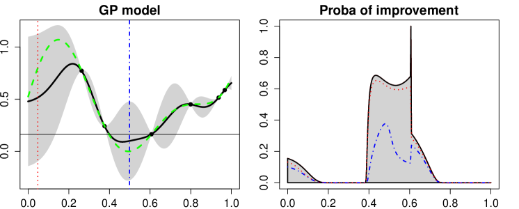
Similarly to the Shannon entropy measure in IAGO, a large volume indicates that the optimum is not yet precisely located (see Figure 1); on the contrary, a small volume indicates that very little can be gained by pursuing the optimization process. Following the stepwise uncertainty reduction paradigm, this volume is an uncertainty measure related to our objective (finding the minimizer of y𝑦y); minimizing the uncertainty amounts to solving the optimization problem.

The probability pn​(𝐱,ynmin):=ℙ​(Y​(𝐱)≀ynmin|π’œn)assignsubscript𝑝𝑛𝐱superscriptsubscriptπ‘¦π‘›β„™π‘Œπ±conditionalsuperscriptsubscript𝑦𝑛subscriptπ’œπ‘›p_{n}(\mathbf{x},y_{n}^{\min}):=\mathbb{P}\left(Y(\mathbf{x})\leq y_{n}^{\min}|\mathcal{A}_{n}\right), which is often referred to as probability of improvement (Jones, 2001), can be expressed in closed form, and Eq.Β (2) writes:

e​vn=βˆ«π•pn​(𝐱,ynmin)​𝑑𝐱=βˆ«π•Ξ¦β€‹(ynminβˆ’mn​(𝐱)sn​(𝐱))​𝑑𝐱,𝑒subscript𝑣𝑛subscript𝕏subscript𝑝𝑛𝐱superscriptsubscript𝑦𝑛differential-d𝐱subscript𝕏Φsuperscriptsubscript𝑦𝑛subscriptπ‘šπ‘›π±subscript𝑠𝑛𝐱differential-d𝐱ev_{n}=\int_{\mathbb{X}}p_{n}(\mathbf{x},y_{n}^{\min})d\mathbf{x}=\int_{\mathbb{X}}\Phi\left(\frac{y_{n}^{\min}-m_{n}(\mathbf{x})}{s_{n}(\mathbf{x})}\right)d\mathbf{x}, (3)

where Ξ¦(.)\Phi(.) is the cumulative distribution function (CDF) of the standard Gaussian distribution. Hypothesizing that a measurement yn+1subscript𝑦𝑛1y_{n+1} is performed at a point 𝐱n+1subscript𝐱𝑛1\mathbf{x}_{n+1}, its benefit can be measured by the reduction of the expected volume of excursion set Ξ”=e​vnβˆ’e​vn+1Δ𝑒subscript𝑣𝑛𝑒subscript𝑣𝑛1\Delta=ev_{n}-ev_{n+1}, with:

e​vn+1𝑒subscript𝑣𝑛1\displaystyle ev_{n+1} =\displaystyle= βˆ«π•pn+1​(𝐱,min⁑(ynmin,yn+1))​𝑑𝐱subscript𝕏subscript𝑝𝑛1𝐱superscriptsubscript𝑦𝑛subscript𝑦𝑛1differential-d𝐱\displaystyle\int_{\mathbb{X}}p_{n+1}(\mathbf{x},\min\left(y_{n}^{\min},y_{n+1}\right))d\mathbf{x}
=\displaystyle= βˆ«π•Ξ¦β€‹(min⁑(ynmin,yn+1)βˆ’mn+1​(𝐱)sn+1​(𝐱))​𝑑𝐱.subscript𝕏Φsuperscriptsubscript𝑦𝑛subscript𝑦𝑛1subscriptπ‘šπ‘›1𝐱subscript𝑠𝑛1𝐱differential-d𝐱\displaystyle\int_{\mathbb{X}}\Phi\left(\frac{\min\left(y_{n}^{\min},y_{n+1}\right)-m_{n+1}(\mathbf{x})}{s_{n+1}(\mathbf{x})}\right)d\mathbf{x}.

Of course, e​vn+1𝑒subscript𝑣𝑛1ev_{n+1} cannot be known exactly without evaluating yn+1subscript𝑦𝑛1y_{n+1}. However, we show in the following that its expectation can be calculated in closed form, leading to a suitable infill criterion. To do so, we first formulate a series of propositions in the next subsection.

3.2 Probabilities updates

An interesting property of the GP model is that, when a new observation yn+1=y​(𝐱n+1)subscript𝑦𝑛1𝑦subscript𝐱𝑛1y_{n+1}=y(\mathbf{x}_{n+1}) is added to the training set, its new predictive distribution can be expressed simply as a function of the old one (Emery, 2009):

mn+1​(𝐱)subscriptπ‘šπ‘›1𝐱\displaystyle m_{n+1}(\mathbf{x}) =\displaystyle= mn​(𝐱)+cn​(𝐱,𝐱n+1)cn​(𝐱n+1,𝐱n+1)​(yn+1βˆ’mn​(𝐱n+1));subscriptπ‘šπ‘›π±subscript𝑐𝑛𝐱subscript𝐱𝑛1subscript𝑐𝑛subscript𝐱𝑛1subscript𝐱𝑛1subscript𝑦𝑛1subscriptπ‘šπ‘›subscript𝐱𝑛1\displaystyle m_{n}(\mathbf{x})+\frac{c_{n}(\mathbf{x},\mathbf{x}_{n+1})}{c_{n}(\mathbf{x}_{n+1},\mathbf{x}_{n+1})}\left({y}_{n+1}-m_{n}\left(\mathbf{x}_{n+1}\right)\right);
sn+12​(𝐱)superscriptsubscript𝑠𝑛12𝐱\displaystyle s_{n+1}^{2}(\mathbf{x}) =\displaystyle= sn2​(𝐱)βˆ’cn​(𝐱,𝐱n+1)2sn2​(𝐱n+1).superscriptsubscript𝑠𝑛2𝐱subscript𝑐𝑛superscript𝐱subscript𝐱𝑛12superscriptsubscript𝑠𝑛2subscript𝐱𝑛1\displaystyle s_{n}^{2}(\mathbf{x})-\frac{c_{n}(\mathbf{x},\mathbf{x}_{n+1})^{2}}{s_{n}^{2}(\mathbf{x}_{n+1})}. (4)

Note that only mn+1​(𝐱)subscriptπ‘šπ‘›1𝐱m_{n+1}(\mathbf{x}) depends on the value of the new observation yn+1subscript𝑦𝑛1{y}_{n+1}. Now, conditionally on the n𝑛n first observations, Yn+1subscriptπ‘Œπ‘›1Y_{n+1} is a random variable (as the new observation has not yet been performed) with its moments given by the GP model:

Yn+1βˆΌπ’©β€‹(mn​(𝐱n+1),sn2​(𝐱n+1)).similar-tosubscriptπ‘Œπ‘›1𝒩subscriptπ‘šπ‘›subscript𝐱𝑛1superscriptsubscript𝑠𝑛2subscript𝐱𝑛1Y_{n+1}\sim\mathcal{N}\left(m_{n}(\mathbf{x}_{n+1}),s_{n}^{2}(\mathbf{x}_{n+1})\right).

We can then define the future expectation Mn+1​(𝐱)subscript𝑀𝑛1𝐱M_{n+1}(\mathbf{x}) (or any quantity depending on it) as a random variable conditionally on π’œnsubscriptπ’œπ‘›\mathcal{A}_{n} and on the fact that the next observation will be at 𝐱n+1subscript𝐱𝑛1\mathbf{x}_{n+1}. This applies to any quantity depending on Yn+1subscriptπ‘Œπ‘›1Y_{n+1} or Mn+1​(𝐱)subscript𝑀𝑛1𝐱M_{n+1}(\mathbf{x}), for instance, the probability of being below a threshold aβˆˆβ„π‘Žβ„a\in\mathbb{R}:

Pn+1​(𝐱,a)=Φ​(aβˆ’Mn+1​(𝐱)sn+1​(𝐱)).subscript𝑃𝑛1π±π‘ŽΞ¦π‘Žsubscript𝑀𝑛1𝐱subscript𝑠𝑛1𝐱P_{n+1}(\mathbf{x},a)=\Phi\left(\frac{a-M_{n+1}(\mathbf{x})}{s_{n+1}(\mathbf{x})}\right).
Proposition 3.1.

Without any restriction on the value of Yn+1subscriptπ‘Œπ‘›1Y_{n+1}, the expectation of the future probability of being below the threshold is equal to the current probability:

ℙ​(Y​(𝐱)≀a|π’œn,Y​(𝐱n+1)=Yn+1)β„™π‘Œπ±conditionalπ‘Žsubscriptπ’œπ‘›π‘Œsubscript𝐱𝑛1subscriptπ‘Œπ‘›1\displaystyle\mathbb{P}\left(Y(\mathbf{x})\leq a|\mathcal{A}_{n},Y(\mathbf{x}_{n+1})=Y_{n+1}\right) =\displaystyle= 𝔼​[Pn+1​(𝐱,a)|π’œn]𝔼delimited-[]conditionalsubscript𝑃𝑛1π±π‘Žsubscriptπ’œπ‘›\displaystyle\mathbb{E}\left[P_{n+1}(\mathbf{x},a)\big{|}\mathcal{A}_{n}\right]
=\displaystyle= pn​(𝐱,a).subscriptπ‘π‘›π±π‘Ž\displaystyle p_{n}(\mathbf{x},a).
Proposition 3.2.

Conditioning further by Yn+1≀bsubscriptπ‘Œπ‘›1𝑏Y_{n+1}\leq b, the probability expectation writes in simple form using the Gaussian bivariate CDF:

q​(𝐱,b,a)π‘žπ±π‘π‘Ž\displaystyle q(\mathbf{x},b,a) :=assign\displaystyle:= β„™[Y(𝐱)≀a|π’œn,Y(𝐱n+1)=Yn+1,Yn+1≀b]\displaystyle\mathbb{P}\left[Y(\mathbf{x})\leq a\big{|}\mathcal{A}_{n},Y(\mathbf{x}_{n+1})=Y_{n+1},Y_{n+1}\leq b\right] (5)
Γ—\displaystyle\times ℙ​[Yn+1≀b|π’œn]β„™delimited-[]subscriptπ‘Œπ‘›1conditional𝑏subscriptπ’œπ‘›\displaystyle\mathbb{P}\left[Y_{n+1}\leq b\big{|}\mathcal{A}_{n}\right]
=\displaystyle= 𝔼​[Pn+1​(𝐱,a)Γ—πŸ™Yn+1≀b|π’œn]𝔼delimited-[]conditionalsubscript𝑃𝑛1π±π‘Žsubscript1subscriptπ‘Œπ‘›1𝑏subscriptπ’œπ‘›\displaystyle\mathbb{E}\left[P_{n+1}(\mathbf{x},a)\times\mathbbmss{1}_{Y_{n+1}\leq b}\big{|}\mathcal{A}_{n}\right]
=\displaystyle= πš½Οβ€‹(bΒ―,a~),subscriptπš½πœŒΒ―π‘~π‘Ž\displaystyle\boldsymbol{\Phi}_{\rho}\left(\bar{b},\tilde{a}\right),

where 𝚽ρsubscript𝚽𝜌\boldsymbol{\Phi}_{\rho} is the Gaussian bivariate CDF with zero mean and covariance [1ρρ1]delimited-[]matrix1𝜌𝜌1\left[\begin{matrix}1&\rho\\ \rho&1\end{matrix}\right], bΒ―=bβˆ’mn​(𝐱n+1)sn​(𝐱n+1)¯𝑏𝑏subscriptπ‘šπ‘›subscript𝐱𝑛1subscript𝑠𝑛subscript𝐱𝑛1\bar{b}=\frac{b-m_{n}(\mathbf{x}_{n+1})}{s_{n}(\mathbf{x}_{n+1})}, a~=aβˆ’mn​(𝐱)sn​(𝐱)~π‘Žπ‘Žsubscriptπ‘šπ‘›π±subscript𝑠𝑛𝐱\tilde{a}=\frac{a-m_{n}(\mathbf{x})}{s_{n}(\mathbf{x})} and ρ=cn​(𝐱,𝐱n+1)sn​(𝐱n+1)​sn​(𝐱).𝜌subscript𝑐𝑛𝐱subscript𝐱𝑛1subscript𝑠𝑛subscript𝐱𝑛1subscript𝑠𝑛𝐱\rho=\frac{c_{n}(\mathbf{x},\mathbf{x}_{n+1})}{s_{n}(\mathbf{x}_{n+1})s_{n}(\mathbf{x})}.

Corollary 3.3.

Similarly, conditioning by Yn+1β‰₯bsubscriptπ‘Œπ‘›1𝑏Y_{n+1}\geq b leads to:

r​(𝐱,b,a)π‘Ÿπ±π‘π‘Ž\displaystyle r(\mathbf{x},b,a) :=assign\displaystyle:= β„™[Y(𝐱)≀a|π’œn,Y(𝐱n+1)=Yn+1,Yn+1β‰₯b]\displaystyle\mathbb{P}\big{[}Y(\mathbf{x})\leq a\big{|}\mathcal{A}_{n},Y(\mathbf{x}_{n+1})=Y_{n+1},Y_{n+1}\geq b\big{]} (6)
Γ—\displaystyle\times ℙ​[Yn+1β‰₯b|π’œn]β„™delimited-[]subscriptπ‘Œπ‘›1conditional𝑏subscriptπ’œπ‘›\displaystyle\mathbb{P}\big{[}Y_{n+1}\geq b\big{|}\mathcal{A}_{n}\big{]}
=\displaystyle= πš½βˆ’Οβ€‹(βˆ’bΒ―,a~).subscriptπš½πœŒΒ―π‘~π‘Ž\displaystyle\boldsymbol{\Phi}_{-\rho}\left(-\bar{b},\tilde{a}\right).

The final proposition resembles Proposition 3.2, but the fixed threshold aπ‘Ža is here replaced by Yn+1subscriptπ‘Œπ‘›1Y_{n+1}:

Proposition 3.4.

The expectation of the probability that Y​(𝐱)π‘Œπ±Y(\mathbf{x}) is smaller than Yn+1subscriptπ‘Œπ‘›1Y_{n+1}, conditionally on Yn+1≀bsubscriptπ‘Œπ‘›1𝑏Y_{n+1}\leq b, is given by:

h​(𝐱,b)β„Žπ±π‘\displaystyle h(\mathbf{x},b) :=assign\displaystyle:= β„™[Y(𝐱)≀Yn+1|π’œn,Y(𝐱n+1)\displaystyle\mathbb{P}\big{[}Y(\mathbf{x})\leq Y_{n+1}|\mathcal{A}_{n},Y(\mathbf{x}_{n+1}) (7)
=\displaystyle= Yn+1,Yn+1≀b]β„™[Yn+1≀b|π’œn]\displaystyle Y_{n+1},Y_{n+1}\leq b\big{]}\mathbb{P}\big{[}Y_{n+1}\leq b\big{|}\mathcal{A}_{n}\big{]}
=\displaystyle= 𝔼​[Pn+1​(𝐱,Yn+1)Γ—πŸ™Yn+1≀b|π’œn]𝔼delimited-[]conditionalsubscript𝑃𝑛1𝐱subscriptπ‘Œπ‘›1subscript1subscriptπ‘Œπ‘›1𝑏subscriptπ’œπ‘›\displaystyle\mathbb{E}\left[P_{n+1}(\mathbf{x},Y_{n+1})\times\mathbbmss{1}_{Y_{n+1}\leq b}\big{|}\mathcal{A}_{n}\right]
=\displaystyle= πš½Ξ½β€‹(bΒ―,Ξ·),subscriptπš½πœˆΒ―π‘πœ‚\displaystyle\boldsymbol{\Phi}_{\nu}\left(\bar{b},\eta\right),

with:

Ξ·πœ‚\displaystyle\eta =\displaystyle= mn​(𝐱n+1)βˆ’mn​(𝐱)sn2​(𝐱)+sn2​(𝐱n+1)βˆ’2​cn​(𝐱,𝐱n+1)​ andsubscriptπ‘šπ‘›subscript𝐱𝑛1subscriptπ‘šπ‘›π±superscriptsubscript𝑠𝑛2𝐱superscriptsubscript𝑠𝑛2subscript𝐱𝑛12subscript𝑐𝑛𝐱subscript𝐱𝑛1Β and\displaystyle\frac{m_{n}(\mathbf{x}_{n+1})-m_{n}(\mathbf{x})}{\sqrt{s_{n}^{2}(\mathbf{x})+s_{n}^{2}(\mathbf{x}_{n+1})-2c_{n}(\mathbf{x},\mathbf{x}_{n+1})}}\text{ and }
ν𝜈\displaystyle\nu =\displaystyle= cn​(𝐱,𝐱n+1)βˆ’sn2​(𝐱n+1)sn​(𝐱n+1)​sn2​(𝐱)+sn2​(𝐱n+1)βˆ’2​cn​(𝐱,𝐱n+1).subscript𝑐𝑛𝐱subscript𝐱𝑛1superscriptsubscript𝑠𝑛2subscript𝐱𝑛1subscript𝑠𝑛subscript𝐱𝑛1superscriptsubscript𝑠𝑛2𝐱superscriptsubscript𝑠𝑛2subscript𝐱𝑛12subscript𝑐𝑛𝐱subscript𝐱𝑛1\displaystyle\frac{c_{n}(\mathbf{x},\mathbf{x}_{n+1})-s_{n}^{2}(\mathbf{x}_{n+1})}{s_{n}(\mathbf{x}_{n+1})\sqrt{s_{n}^{2}(\mathbf{x})+s_{n}^{2}(\mathbf{x}_{n+1})-2c_{n}(\mathbf{x},\mathbf{x}_{n+1})}}.

All the proofs are reported in Appendix A.

3.3 A Stepwise uncertainty reduction criterion

Coming back to the SUR criterion, at step n𝑛n the future volume of excursion set E​Vn+1𝐸subscript𝑉𝑛1EV_{n+1} is a random variable, and its expectation is:

E​E​V​(𝐱n+1)𝐸𝐸𝑉subscript𝐱𝑛1\displaystyle EEV(\mathbf{x}_{n+1}) :=assign\displaystyle:= 𝔼​(E​Vn+1|π’œn,Y​(𝐱n+1)=Yn+1)𝔼conditional𝐸subscript𝑉𝑛1subscriptπ’œπ‘›π‘Œsubscript𝐱𝑛1subscriptπ‘Œπ‘›1\displaystyle\mathbb{E}\left(EV_{n+1}\big{|}\mathcal{A}_{n},Y(\mathbf{x}_{n+1})=Y_{n+1}\right)
=\displaystyle= βˆ«π•π”Ό[Ξ¦(min⁑(ynmin,Yn+1)βˆ’Mn+1​(𝐱)sn+1​(𝐱))\displaystyle\int_{\mathbb{X}}\mathbb{E}\Big{[}\Phi\left(\frac{\min\left(y_{n}^{\min},Y_{n+1}\right)-M_{n+1}(\mathbf{x})}{s_{n+1}(\mathbf{x})}\right)
|π’œn,Y(𝐱n+1)=Yn+1]d𝐱.\displaystyle\big{|}\mathcal{A}_{n},Y(\mathbf{x}_{n+1})=Y_{n+1}\Big{]}d\mathbf{x}.

Let φ​(yn+1)πœ‘subscript𝑦𝑛1\varphi\left(y_{n+1}\right) be the probability density function (PDF) of Yn+1subscriptπ‘Œπ‘›1Y_{n+1} conditionally on π’œnsubscriptπ’œπ‘›\mathcal{A}_{n}. We have:

E​E​V​(𝐱n+1)𝐸𝐸𝑉subscript𝐱𝑛1\displaystyle EEV(\mathbf{x}_{n+1})
=\displaystyle= βˆ«π•βˆ«β„Ξ¦β€‹(min⁑(ynmin,yn+1)βˆ’mn+1​(𝐱)sn+1​(𝐱))​𝑑φ​(yn+1)​𝑑𝐱subscript𝕏subscriptℝΦsuperscriptsubscript𝑦𝑛subscript𝑦𝑛1subscriptπ‘šπ‘›1𝐱subscript𝑠𝑛1𝐱differential-dπœ‘subscript𝑦𝑛1differential-d𝐱\displaystyle\int_{\mathbb{X}}\int_{\mathbb{R}}\Phi\left(\frac{\min\left(y_{n}^{\min},y_{n+1}\right)-m_{n+1}(\mathbf{x})}{s_{n+1}(\mathbf{x})}\right)d\varphi\left(y_{n+1}\right)d\mathbf{x}
=\displaystyle= βˆ«π•[βˆ«βˆ’βˆžynminΞ¦(yn+1βˆ’mn+1​(𝐱)sn+1​(𝐱))\displaystyle\int_{\mathbb{X}}\big{[}\int_{-\infty}^{y_{n}^{\min}}\Phi\left(\frac{y_{n+1}-m_{n+1}(\mathbf{x})}{s_{n+1}(\mathbf{x})}\right)
+\displaystyle+ ∫ynmin+∞Φ(ynminβˆ’mn+1​(𝐱)sn+1​(𝐱))dΟ†(yn+1)]d𝐱\displaystyle\int_{y_{n}^{\min}}^{+\infty}\Phi\left(\frac{y_{n}^{\min}-m_{n+1}(\mathbf{x})}{s_{n+1}(\mathbf{x})}\right)d\varphi\left(y_{n+1}\right)\big{]}d\mathbf{x}
=\displaystyle= βˆ«π•[h​(𝐱,ynmin)+r​(𝐱,ynmin,ynmin)]​𝑑𝐱.subscript𝕏delimited-[]β„Žπ±superscriptsubscriptπ‘¦π‘›π‘Ÿπ±superscriptsubscript𝑦𝑛superscriptsubscript𝑦𝑛differential-d𝐱\displaystyle\int_{\mathbb{X}}\left[h(\mathbf{x},y_{n}^{\min})+r(\mathbf{x},y_{n}^{\min},y_{n}^{\min})\right]d\mathbf{x}.

The first term of the integrand is given by Eq.Β (7) in Proposition 3.4, with b=ynmin𝑏superscriptsubscript𝑦𝑛b=y_{n}^{\min}, and the second term is given by Eq.Β (6) in Corrolary 3.3, with a=b=ynminπ‘Žπ‘superscriptsubscript𝑦𝑛a=b=y_{n}^{\min}, hence:

E​E​V​(𝐱n+1)=βˆ«π•[πš½Ξ½β€‹(yΒ―nmin,Ξ·)+πš½Οβ€‹(βˆ’yΒ―nmin,y~nmin)]​𝑑𝐱,𝐸𝐸𝑉subscript𝐱𝑛1subscript𝕏delimited-[]subscript𝚽𝜈superscriptsubscriptΒ―π‘¦π‘›πœ‚subscript𝚽𝜌superscriptsubscript¯𝑦𝑛superscriptsubscript~𝑦𝑛differential-d𝐱EEV(\mathbf{x}_{n+1})=\int_{\mathbb{X}}{\left[\boldsymbol{\Phi}_{\nu}\left(\overline{y}_{n}^{\min},\eta\right)+\boldsymbol{\Phi}_{\rho}\left(-\overline{y}_{n}^{\min},\widetilde{y}_{n}^{\min}\right)\right]d\mathbf{x}}, (8)

with:

yΒ―nmin=(ynminβˆ’mn​(𝐱n+1))/sn​(𝐱n+1)superscriptsubscript¯𝑦𝑛superscriptsubscript𝑦𝑛subscriptπ‘šπ‘›subscript𝐱𝑛1subscript𝑠𝑛subscript𝐱𝑛1\overline{y}_{n}^{\min}={(y_{n}^{\min}-m_{n}(\mathbf{x}_{n+1}))}/{s_{n}(\mathbf{x}_{n+1})}

and

y~nmin=(ynminβˆ’mn​(𝐱))/sn​(𝐱).superscriptsubscript~𝑦𝑛superscriptsubscript𝑦𝑛subscriptπ‘šπ‘›π±subscript𝑠𝑛𝐱\widetilde{y}_{n}^{\min}={(y_{n}^{\min}-m_{n}(\mathbf{x}))}/{s_{n}(\mathbf{x})}.

The SUR optimization strategy consists in adding the experiment that minimizes the expected volume of excursion set (or maximizes the difference), that is, the one-step optimal policy in terms of reduction of the uncertainty on the objective function minimizer:

𝐱n+1=arg⁑min𝐱+βˆˆπ•β‘E​E​V​(𝐱+)subscript𝐱𝑛1subscriptsuperscript𝐱𝕏𝐸𝐸𝑉superscript𝐱\mathbf{x}_{n+1}=\arg\min_{\mathbf{x}^{+}\in\mathbb{X}}EEV(\mathbf{x}^{+}) (9)
  • Remark

    In general, the probability of improvement pn​(𝐱,ynmin)subscript𝑝𝑛𝐱superscriptsubscript𝑦𝑛p_{n}(\mathbf{x},y_{n}^{\min}) is high where the prediction mean mn(.)m_{n}(.) is low and/or the prediction variance sn2(.)s_{n}^{2}(.) is high. Simply choosing points that maximize pn​(𝐱,ynmin)subscript𝑝𝑛𝐱superscriptsubscript𝑦𝑛p_{n}(\mathbf{x},y_{n}^{\min}) is known to be inefficient (Jones, 2001), as it does not consider the amplitude of the gain in the objective function. Here, E​E​V​(𝐱+)𝐸𝐸𝑉superscript𝐱EEV(\mathbf{x}^{+}) strongly depends on the potential gain amplitude. Indeed, minimizing the expected volume relies on two mecanisms: reducing the local uncertainty and lowering the current minimum value (ynminsuperscriptsubscript𝑦𝑛y_{n}^{\min}). The first is achieved by adding measurements in unsampled regions (high sn2(.)s_{n}^{2}(.)), the second in regions where this potential reduction is high. Hence, the E​E​V𝐸𝐸𝑉EEV criterion can be seen as a mixed measure of uncertainty on the current minimum location and of potential gain in the objective function.

3.4 Illustration

Figure 1 illustrates the concept of reduction of volume of excursion on a toy example. A GP model is built on a six-point training set, from which the probability of improvement p6​(𝐱,y6min)subscript𝑝6𝐱subscriptsuperscript𝑦6p_{6}(\mathbf{x},y^{\min}_{6}) is computed for every point in 𝕏=[0,1]𝕏01\mathbb{X}=[0,1]. We see that it can be intepreted as an indicator of the uncertainty we have about the location of the actual minimizer π±βˆ—=0.47superscript𝐱0.47\mathbf{x}^{*}=0.47, as the model can only predict that π±βˆ—superscript𝐱\mathbf{x}^{*} is likely to be between 0.40.40.4 and 0.60.60.6. Then, we consider two candidate points (𝐱+=0.2superscript𝐱0.2\mathbf{x}^{+}=0.2 and 𝐱+=0.5superscript𝐱0.5\mathbf{x}^{+}=0.5) and compute, for each, the expected new probability (integrand in Eq.Β (3.3)). We see that the probability is likely to remain mostly unchanged by adding the measurement at 𝐱+=0.2superscript𝐱0.2\mathbf{x}^{+}=0.2 (which is, indeed, a region with high response value), while it would be considerably reduced by adding a measurement at 𝐱+=0.5superscript𝐱0.5\mathbf{x}^{+}=0.5. In terms of volume of excursion set, we have E​E​V​(0.2)β‰ˆe​v6𝐸𝐸𝑉0.2𝑒subscript𝑣6EEV(0.2)\approx ev_{6} (no reduction), while E​E​V​(0.5)β‰ˆe​v6/3𝐸𝐸𝑉0.5𝑒subscript𝑣63EEV(0.5)\approx ev_{6}/3 (large reduction): the E​E​V𝐸𝐸𝑉EEV criterion clearly indicates 𝐱+=0.5superscript𝐱0.5\mathbf{x}^{+}=0.5 as a better sampling location.

Refer to caption
Figure 1: Illustration of the effect of a new observation on the EV criterion. Left: actual objective function (dotted line), GP model (depicted by its mean in black plain line and 95% confidence interval in grey) based on six observations (black circles). The horizontal line shows the current minimum; the vertical bars are placed at two candidate locations. Right: probability of improvement given by the current model and expected updated probability for each candidate. Adding a point at x+=0.5superscriptπ‘₯0.5x^{+}=0.5 (mixed line) is likely to reduce substantially the probability, while adding a point at x+=0.05superscriptπ‘₯0.05x^{+}=0.05 (dotted line) has little expected effect.

4 Multi-objective optimization by stepwise uncertainty reduction

4.1 Volume of excursion behind the Pareto front

Let 𝐲​(𝐱)=(y(1)​(𝐱),…,y(q)​(𝐱))𝐲𝐱superscript𝑦1𝐱…superscriptπ‘¦π‘žπ±\mathbf{y}(\mathbf{x})=\left(y^{(1)}(\mathbf{x}),\ldots,y^{(q)}(\mathbf{x})\right) be the vector of objective functions to minimize. A point 𝐱𝐱\mathbf{x} dominates another point 𝐱′superscript𝐱′\mathbf{x}^{\prime} if y(k)​(𝐱)≀y(k)​(𝐱′)superscriptπ‘¦π‘˜π±superscriptπ‘¦π‘˜superscript𝐱′y^{(k)}(\mathbf{x})\leq y^{(k)}(\mathbf{x}^{\prime}) for all kπ‘˜k in {1,…,q}1β€¦π‘ž\{1,\ldots,q\}, which we denote by 𝐱′≺𝐱precedessuperscript𝐱′𝐱\mathbf{x}^{\prime}\prec\mathbf{x} in the following. At step n𝑛n, 𝐗n={𝐱1,…,𝐱n}subscript𝐗𝑛subscript𝐱1…subscript𝐱𝑛\mathbf{X}_{n}=\{\mathbf{x}_{1},\ldots,\mathbf{x}_{n}\} is the current experimental set and 𝐘n={𝐲​(𝐱1),…,𝐲​(𝐱n)}subscriptπ˜π‘›π²subscript𝐱1…𝐲subscript𝐱𝑛\mathbf{Y}_{n}=\{\mathbf{y}(\mathbf{x}_{1}),\ldots,\mathbf{y}(\mathbf{x}_{n})\} the corresponding set of measures. The non-dominated subset 𝐗nβˆ—superscriptsubscript𝐗𝑛\mathbf{X}_{n}^{*} of 𝐗nsubscript𝐗𝑛\mathbf{X}_{n} constitutes the current Pareto front (of size m≀nπ‘šπ‘›m\leq n). In the objective space, the corresponding subset 𝐘nβˆ—superscriptsubscriptπ˜π‘›\mathbf{Y}_{n}^{*} separates the regions dominated and not dominated by the experimental set.

Then, we decompose the objective space plane using a tesselation {Ξ©i}i∈{1,…,I}subscriptsubscriptΩ𝑖𝑖1…𝐼\{\Omega_{i}\}_{i\in\{1,\ldots,I\}} of size I=(m+1)q𝐼superscriptπ‘š1π‘žI=(m+1)^{q} (βˆͺi∈IΞ©i=ℝqsubscript𝑖𝐼subscriptΩ𝑖superscriptβ„π‘ž\cup_{i\in I}\Omega_{i}=\mathbb{R}^{q} and ∩i∈IΞ©i=βˆ…subscript𝑖𝐼subscriptΩ𝑖\cap_{i\in I}\Omega_{i}=\emptyset), each cell being a hyperrectangle defined as:

Ξ©i={π²βˆˆβ„q|yiβˆ’(k)≀y(k)<yi+(k),k∈{1,…,q}}.subscriptΩ𝑖conditional-set𝐲superscriptβ„π‘žformulae-sequencesubscriptsuperscriptπ‘¦π‘˜limit-from𝑖superscriptπ‘¦π‘˜subscriptsuperscriptπ‘¦π‘˜limit-fromπ‘–π‘˜1β€¦π‘ž\Omega_{i}=\{\mathbf{y}\in\mathbb{R}^{q}|y^{(k)}_{i-}\leq y^{(k)}<y^{(k)}_{i+},k\in\{1,\ldots,q\}\}.

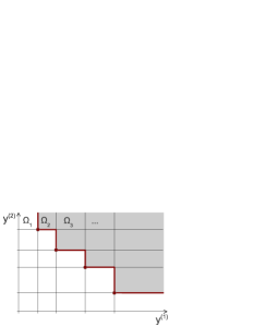
Each couple (yiβˆ’(k),yi+(k))subscriptsuperscriptπ‘¦π‘˜limit-from𝑖subscriptsuperscriptπ‘¦π‘˜limit-from𝑖(y^{(k)}_{i-},y^{(k)}_{i+}) consists of two consecutive values of the vector [βˆ’βˆž,y(k)​(𝐱1βˆ—),…,y(k)​(𝐱mβˆ—),+∞]superscriptπ‘¦π‘˜superscriptsubscript𝐱1…superscriptπ‘¦π‘˜superscriptsubscriptπ±π‘š\left[-\infty,y^{(k)}(\mathbf{x}_{1}^{*}),\ldots,y^{(k)}(\mathbf{x}_{m}^{*}),+\infty\right]. An illustration is given in Figure 2.

A cell Ξ©isubscriptΩ𝑖\Omega_{i} dominates another cell Ξ©jsubscriptΩ𝑗\Omega_{j} (Ξ©jβ‰ΊΞ©iprecedessubscriptΩ𝑗subscriptΩ𝑖\Omega_{j}\prec\Omega_{i}) if any point in Ξ©isubscriptΩ𝑖\Omega_{i} dominates any point in Ξ©jsubscriptΩ𝑗\Omega_{j}, and it partially dominates Ξ©jsubscriptΩ𝑗\Omega_{j} if there exists a point in Ξ©jsubscriptΩ𝑗\Omega_{j} that is dominated by any point in Ξ©isubscriptΩ𝑖\Omega_{i}. Otherwise, we say that Ξ©jsubscriptΩ𝑗\Omega_{j} is not dominated by Ξ©isubscriptΩ𝑖\Omega_{i} (Ξ©jβŠ€Ξ©inot-precedessubscriptΩ𝑗subscriptΩ𝑖\Omega_{j}\not\prec\Omega_{i}).

We denote by Iβˆ—superscript𝐼I^{*} the indices of all the non-dominated cells at step n𝑛n, that is, the cells that are not dominated by any point of 𝐗nβˆ—superscriptsubscript𝐗𝑛\mathbf{X}_{n}^{*}. In two dimensions, the non-dominated cells are located in the bottom left half of the plane (Figure 2).
Refer to caption
Figure 2: Example of Pareto front generated by four points (circles), and associated tesselation. The grey area corresponds to the dominated cells.
Refer to caption
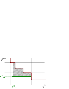
Figure 3: Example of Pareto front modification due to a new measurement. Two points are removed from the Pareto front while the new point is added. The hatched area represents the additional dominated region.

Now, let us assume that GP models are fitted to each objective y(k)y^{(k}). At step n𝑛n, the probability that π˜β€‹(𝐱)𝐘𝐱\mathbf{Y}(\mathbf{x}) belongs to the cell Ξ©isubscriptΩ𝑖\Omega_{i} is:

pni​(𝐱)superscriptsubscript𝑝𝑛𝑖𝐱\displaystyle p_{n}^{i}(\mathbf{x}) =\displaystyle= ℙ​[π˜β€‹(𝐱)∈Ωi|π’œn]β„™delimited-[]𝐘𝐱conditionalsubscriptΩ𝑖subscriptπ’œπ‘›\displaystyle{\mathbb{P}}\left[\mathbf{Y}(\mathbf{x})\in\Omega_{i}\big{|}\mathcal{A}_{n}\right]
=\displaystyle= ∏k=1qΦ​(yi+(k)βˆ’mn(k)​(𝐱)sn(k)​(𝐱))βˆ’Ξ¦β€‹(yiβˆ’(k)βˆ’mn(k)​(𝐱)sn(k)​(𝐱))superscriptsubscriptproductπ‘˜1π‘žΞ¦subscriptsuperscriptπ‘¦π‘˜limit-from𝑖superscriptsubscriptπ‘šπ‘›π‘˜π±superscriptsubscriptπ‘ π‘›π‘˜π±Ξ¦subscriptsuperscriptπ‘¦π‘˜limit-from𝑖superscriptsubscriptπ‘šπ‘›π‘˜π±superscriptsubscriptπ‘ π‘›π‘˜π±\displaystyle\prod_{k=1}^{q}\Phi\left(\frac{y^{(k)}_{i+}-m_{n}^{(k)}(\mathbf{x})}{s_{n}^{(k)}(\mathbf{x})}\right)-\Phi\left(\frac{y^{(k)}_{i-}-m_{n}^{(k)}(\mathbf{x})}{s_{n}^{(k)}(\mathbf{x})}\right)
:=assign\displaystyle:= ∏k=1qpni​(k)superscriptsubscriptproductπ‘˜1π‘žsuperscriptsubscriptπ‘π‘›π‘–π‘˜\displaystyle\prod_{k=1}^{q}p_{n}^{i(k)}

by pairwise independence of Y(1),…,Y(q)superscriptπ‘Œ1…superscriptπ‘Œπ‘žY^{(1)},\ldots,Y^{(q)}. The probability that 𝐱𝐱\mathbf{x} is not dominated by any point of 𝐗nsubscript𝐗𝑛\mathbf{X}_{n} is then the probability that π˜β€‹(𝐱)𝐘𝐱\mathbf{Y}(\mathbf{x}) belongs to one of the non-dominated parts of the objective space. As the Ξ©isubscriptΩ𝑖\Omega_{i}’s are disjoint, it is equal to:

ℙ​(π±βŠ€π—n|π’œn)=βˆ‘i∈Iβˆ—pni​(𝐱).β„™not-precedes𝐱conditionalsubscript𝐗𝑛subscriptπ’œπ‘›subscript𝑖superscript𝐼superscriptsubscript𝑝𝑛𝑖𝐱{\mathbb{P}}(\mathbf{x}\not\prec\mathbf{X}_{n}\big{|}\mathcal{A}_{n})=\sum_{i\in I^{*}}p_{n}^{i}(\mathbf{x}). (10)

Finally, the volume of the excursion sets behind the Pareto front is equal to the integral of this probability over 𝕏𝕏\mathbb{X}:

e​vn𝑒subscript𝑣𝑛\displaystyle ev_{n} =\displaystyle= βˆ«π•β„™β€‹(π±βŠ€π—n|π’œn)​𝑑𝐱subscript𝕏ℙnot-precedes𝐱conditionalsubscript𝐗𝑛subscriptπ’œπ‘›differential-d𝐱\displaystyle\int_{\mathbb{X}}{\mathbb{P}}(\mathbf{x}\not\prec\mathbf{X}_{n}\big{|}\mathcal{A}_{n})d\mathbf{x} (11)
=\displaystyle= βˆ«π•βˆ‘i∈Iβˆ—pni​(𝐱)​d​𝐱=βˆ‘i∈Iβˆ—βˆ«π•pni​(𝐱)​𝑑𝐱.subscript𝕏subscript𝑖superscript𝐼superscriptsubscript𝑝𝑛𝑖𝐱𝑑𝐱subscript𝑖superscript𝐼subscript𝕏superscriptsubscript𝑝𝑛𝑖𝐱differential-d𝐱\displaystyle\int_{\mathbb{X}}\sum_{i\in I^{*}}p_{n}^{i}(\mathbf{x})d\mathbf{x}=\sum_{i\in I^{*}}\int_{\mathbb{X}}p_{n}^{i}(\mathbf{x})d\mathbf{x}.

When e​vn𝑒subscript𝑣𝑛ev_{n} is high, a large proportion of the design space is likely to be better than the current Pareto set; inversely, when 𝐗nβˆ—superscriptsubscript𝐗𝑛\mathbf{X}_{n}^{*} approaches the actual Pareto set π•βˆ—superscript𝕏\mathbb{X}^{*}, the volume tends to zero. Hence, it defines naturally an uncertainty indicator for a SUR strategy.

4.2 SUR criterion derivation

Now, let us consider that a measurement 𝐲n+1subscript𝐲𝑛1\mathbf{y}_{n+1} is performed at a point 𝐱n+1subscript𝐱𝑛1\mathbf{x}_{n+1}. Compared to step n𝑛n, the volume e​v𝑒𝑣ev is modified by two means. First, the new measurement will modify the quantities mn(k)​(𝐱)superscriptsubscriptπ‘šπ‘›π‘˜π±m_{n}^{(k)}(\mathbf{x}), sn(k)​(𝐱)superscriptsubscriptπ‘ π‘›π‘˜π±s_{n}^{(k)}(\mathbf{x}) (k∈{1,…,q}π‘˜1β€¦π‘žk\in\{1,\ldots,q\}), hence, the probabilities pni​(𝐱)superscriptsubscript𝑝𝑛𝑖𝐱p_{n}^{i}(\mathbf{x}). Second, if the new measurement is not dominated by the current Pareto set, it modifies the Pareto optimal front, as the new value 𝐲​(𝐱n+1)𝐲subscript𝐱𝑛1\mathbf{y}(\mathbf{x}_{n+1}) is added to π˜βˆ—superscript𝐘\mathbf{Y}^{*} and the values of π˜βˆ—superscript𝐘\mathbf{Y}^{*} dominated by 𝐲​(𝐱n+1)𝐲subscript𝐱𝑛1\mathbf{y}(\mathbf{x}_{n+1}) (if they exist) are removed. An example of such update is given in Figure 3.

Focusing on the probability that a point remains non-dominated (Eq.Β (10)), accounting for the modifications of the models is relatively easy (that is, computing the quantity pn+1i(.)p_{n+1}^{i}(.)), but accounting for modifications in the Pareto front is complex, as both the number of elements and their values might change. To address this issue, we consider that the updated probability ℙ​(π±βŠ€π—n+1|π’œn+1)β„™not-precedes𝐱conditionalsubscript𝐗𝑛1subscriptπ’œπ‘›1{\mathbb{P}}(\mathbf{x}\not\prec\mathbf{X}_{n+1}\big{|}\mathcal{A}_{n+1}) can be computed using the same sum as for ℙ​(π±βŠ€π—n|π’œn)β„™not-precedes𝐱conditionalsubscript𝐗𝑛subscriptπ’œπ‘›{\mathbb{P}}(\mathbf{x}\not\prec\mathbf{X}_{n}\big{|}\mathcal{A}_{n}) (Eq.Β (10)) by modifying its elements pni​(𝐱)superscriptsubscript𝑝𝑛𝑖𝐱p_{n}^{i}(\mathbf{x}):

ℙ​(π±βŠ€π—n+1|π’œn+1)=βˆ‘i∈Iβˆ—p~n+1i​(𝐱),β„™not-precedes𝐱conditionalsubscript𝐗𝑛1subscriptπ’œπ‘›1subscript𝑖superscript𝐼superscriptsubscript~𝑝𝑛1𝑖𝐱{\mathbb{P}}(\mathbf{x}\not\prec\mathbf{X}_{n+1}\big{|}\mathcal{A}_{n+1})=\sum_{i\in I^{*}}\tilde{p}_{n+1}^{i}(\mathbf{x}),

with

p~n+1i​(𝐱)=ℙ​(π±βŠ€π—n+1βˆ©π˜β€‹(𝐱)∈Ωi|π’œn,𝐲​(𝐱n+1)=𝐲n+1)superscriptsubscript~𝑝𝑛1𝑖𝐱ℙnot-precedes𝐱subscript𝐗𝑛1𝐘𝐱conditionalsubscriptΩ𝑖subscriptπ’œπ‘›π²subscript𝐱𝑛1subscript𝐲𝑛1\tilde{p}_{n+1}^{i}(\mathbf{x})={\mathbb{P}}\Big{(}\mathbf{x}\not\prec\mathbf{X}_{n+1}\cap\mathbf{Y}(\mathbf{x})\in\Omega_{i}\Big{|}\mathcal{A}_{n},\mathbf{y}(\mathbf{x}_{n+1})=\mathbf{y}_{n+1}\Big{)}

and the Ξ©isubscriptΩ𝑖\Omega_{i}’s defined using 𝐘nβˆ—superscriptsubscriptπ˜π‘›\mathbf{Y}_{n}^{*} (not 𝐘n+1βˆ—superscriptsubscriptπ˜π‘›1\mathbf{Y}_{n+1}^{*}).

Seing from step n𝑛n, the P~n+1j​(𝐱)superscriptsubscript~𝑃𝑛1𝑗𝐱\tilde{P}_{n+1}^{j}(\mathbf{x}) are random, as

Y​(𝐱n+1)(k)βˆΌπ’©β€‹(mn(k)​(𝐱n+1),sn(k)​2​(𝐱n+1)),similar-toπ‘Œsuperscriptsubscript𝐱𝑛1π‘˜π’©superscriptsubscriptπ‘šπ‘›π‘˜subscript𝐱𝑛1superscriptsubscriptπ‘ π‘›π‘˜2subscript𝐱𝑛1Y(\mathbf{x}_{n+1})^{(k)}\sim\mathcal{N}\left(m_{n}^{(k)}(\mathbf{x}_{n+1}),s_{n}^{(k)2}(\mathbf{x}_{n+1})\right),

βˆ€k∈{1,…,q}for-allπ‘˜1β€¦π‘ž\forall k\in\{1,\ldots,q\}.

The expectation of the new volume is then:

E​E​V​(𝐱n+1)𝐸𝐸𝑉subscript𝐱𝑛1\displaystyle EEV(\mathbf{x}_{n+1}) =\displaystyle= 𝔼​[βˆ«π•βˆ‘j∈Iβˆ—P~n+1j​(𝐱)​d​𝐱]𝔼delimited-[]subscript𝕏subscript𝑗superscript𝐼superscriptsubscript~𝑃𝑛1𝑗𝐱𝑑𝐱\displaystyle\mathbb{E}\left[\int_{\mathbb{X}}\sum_{j\in I^{*}}\tilde{P}_{n+1}^{j}(\mathbf{x})d\mathbf{x}\right]
=\displaystyle= βˆ‘j∈Iβˆ—βˆ«π•π”Όβ€‹[P~n+1j​(𝐱)]​𝑑𝐱.subscript𝑗superscript𝐼subscript𝕏𝔼delimited-[]superscriptsubscript~𝑃𝑛1𝑗𝐱differential-d𝐱\displaystyle\sum_{j\in I^{*}}\int_{\mathbb{X}}\mathbb{E}\left[\tilde{P}_{n+1}^{j}(\mathbf{x})\right]d\mathbf{x}.

This expression can be decomposed by conditioning on the range values of the new observation (using the fact that the Ξ©isubscriptΩ𝑖\Omega_{i}’s are disjoint):

𝔼​[P~n+1j​(𝐱)]𝔼delimited-[]superscriptsubscript~𝑃𝑛1𝑗𝐱\displaystyle\mathbb{E}\left[\tilde{P}_{n+1}^{j}(\mathbf{x})\right]
=βˆ‘i∈Iβ„™n+1[\displaystyle=\sum_{i\in I}{\mathbb{P}}_{n+1}\Big{[} 𝐱𝐱\displaystyle\mathbf{x} βŠ€π—n+1∩𝐘(𝐱)∈Ωj|𝐘n+1∈Ωi]\displaystyle\not\prec\mathbf{X}_{n+1}\cap\mathbf{Y}(\mathbf{x})\in\Omega_{j}\Big{|}\mathbf{Y}_{n+1}\in\Omega_{i}\Big{]}
Γ—\displaystyle\times β„™n+1​[𝐘n+1∈Ωi]subscriptℙ𝑛1delimited-[]subscriptπ˜π‘›1subscriptΩ𝑖\displaystyle{\mathbb{P}}_{n+1}\Big{[}\mathbf{Y}_{n+1}\in\Omega_{i}\Big{]}
:=βˆ‘i∈Ipi​j​(𝐱),assignabsentsubscript𝑖𝐼subscript𝑝𝑖𝑗𝐱\displaystyle:=\sum_{i\in I}p_{ij}(\mathbf{x}),

where β„™n+1subscriptℙ𝑛1{\mathbb{P}}_{n+1} is the probability conditional on
(π’œn,π˜β€‹(𝐱n+1)=𝐘n+1)subscriptπ’œπ‘›π˜subscript𝐱𝑛1subscriptπ˜π‘›1\Big{(}\mathcal{A}_{n},\mathbf{Y}(\mathbf{x}_{n+1})=\mathbf{Y}_{n+1}\Big{)}.

We first note from Proposition 3.1 that

β„™n+1​[𝐘n+1∈Ωi]=pni​(𝐱n+1).subscriptℙ𝑛1delimited-[]subscriptπ˜π‘›1subscriptΩ𝑖superscriptsubscript𝑝𝑛𝑖subscript𝐱𝑛1{\mathbb{P}}_{n+1}\left[\mathbf{Y}_{n+1}\in\Omega_{i}\right]=p_{n}^{i}(\mathbf{x}_{n+1}).

Then, leaving aside non-domination, the probability that π˜β€‹(𝐱)𝐘𝐱\mathbf{Y}(\mathbf{x}) belongs to Ξ©jsubscriptΩ𝑗\Omega_{j} knowing that 𝐘n+1subscriptπ˜π‘›1\mathbf{Y}_{n+1} belongs to Ξ©isubscriptΩ𝑖\Omega_{i} is given by:

β„™n+1​[π˜β€‹(𝐱)∈Ωj|𝐘n+1∈Ωi]Γ—pni​(𝐱n+1)=∏k=1qbi​j(k)​(𝐱),subscriptℙ𝑛1delimited-[]𝐘𝐱conditionalsubscriptΩ𝑗subscriptπ˜π‘›1subscriptΩ𝑖superscriptsubscript𝑝𝑛𝑖subscript𝐱𝑛1superscriptsubscriptproductπ‘˜1π‘žsuperscriptsubscriptπ‘π‘–π‘—π‘˜π±{\mathbb{P}}_{n+1}\Big{[}\mathbf{Y}(\mathbf{x})\in\Omega_{j}\Big{|}\mathbf{Y}_{n+1}\in\Omega_{i}\Big{]}\times p_{n}^{i}(\mathbf{x}_{n+1})=\prod_{k=1}^{q}b_{ij}^{(k)}(\mathbf{x}),

with:

bi​j(k)​(𝐱)superscriptsubscriptπ‘π‘–π‘—π‘˜π±\displaystyle b_{ij}^{(k)}(\mathbf{x}) =\displaystyle= β„™n+1​[yjβˆ’(k)≀Y(k)​(𝐱)​<yj+(k)|​yiβˆ’(k)≀Yn+1(k)<yi+(k)]subscriptℙ𝑛1delimited-[]subscriptsuperscriptπ‘¦π‘˜limit-from𝑗superscriptπ‘Œπ‘˜π±brasubscriptsuperscriptπ‘¦π‘˜limit-from𝑗subscriptsuperscriptπ‘¦π‘˜limit-from𝑖subscriptsuperscriptπ‘Œπ‘˜π‘›1subscriptsuperscriptπ‘¦π‘˜limit-from𝑖\displaystyle{\mathbb{P}}_{n+1}\Big{[}y^{(k)}_{j-}\leq Y^{(k)}(\mathbf{x})<y^{(k)}_{j+}\Big{|}y^{(k)}_{i-}\leq Y^{(k)}_{n+1}<y^{(k)}_{i+}\Big{]}
Γ—\displaystyle\times pni​(k)​(𝐱n+1),superscriptsubscriptπ‘π‘›π‘–π‘˜subscript𝐱𝑛1\displaystyle p_{n}^{i(k)}(\mathbf{x}_{n+1}),
pni​(k)​(𝐱n+1)=β„™n​[yiβˆ’(k)≀Yn+1(k)<yi+(k)],superscriptsubscriptπ‘π‘›π‘–π‘˜subscript𝐱𝑛1subscriptℙ𝑛delimited-[]subscriptsuperscriptπ‘¦π‘˜limit-from𝑖subscriptsuperscriptπ‘Œπ‘˜π‘›1subscriptsuperscriptπ‘¦π‘˜limit-from𝑖\displaystyle p_{n}^{i(k)}(\mathbf{x}_{n+1})={\mathbb{P}}_{n}\left[y^{(k)}_{i-}\leq Y^{(k)}_{n+1}<y^{(k)}_{i+}\right],

by pairwise independence of Y(1),…,Y(q)superscriptπ‘Œ1…superscriptπ‘Œπ‘žY^{(1)},\ldots,Y^{(q)}. We show in Appendix B that bi​j(k)​(𝐱)superscriptsubscriptπ‘π‘–π‘—π‘˜π±b_{ij}^{(k)}(\mathbf{x}) can be expressed in closed form as:

bi​j(k)​(𝐱)superscriptsubscriptπ‘π‘–π‘—π‘˜π±\displaystyle b_{ij}^{(k)}(\mathbf{x}) =\displaystyle= 𝚽ρ(k)​(yΒ―i+(k),y~j+(k))βˆ’πš½Ο(k)​(yΒ―i+(k),y~jβˆ’(k))superscriptsubscriptπš½πœŒπ‘˜subscriptsuperscriptΒ―π‘¦π‘˜limit-from𝑖subscriptsuperscript~π‘¦π‘˜limit-from𝑗superscriptsubscriptπš½πœŒπ‘˜subscriptsuperscriptΒ―π‘¦π‘˜limit-from𝑖subscriptsuperscript~π‘¦π‘˜limit-from𝑗\displaystyle\boldsymbol{\Phi}_{\rho}^{(k)}\left(\overline{y}^{(k)}_{i+},\widetilde{y}^{(k)}_{j+}\right)-\boldsymbol{\Phi}_{\rho}^{(k)}\left(\overline{y}^{(k)}_{i+},\widetilde{y}^{(k)}_{j-}\right)
βˆ’\displaystyle- 𝚽ρ(k)​(yΒ―iβˆ’(k),y~j+(k))+𝚽ρ(k)​(yΒ―iβˆ’(k),y~jβˆ’(k))superscriptsubscriptπš½πœŒπ‘˜subscriptsuperscriptΒ―π‘¦π‘˜limit-from𝑖subscriptsuperscript~π‘¦π‘˜limit-from𝑗superscriptsubscriptπš½πœŒπ‘˜subscriptsuperscriptΒ―π‘¦π‘˜limit-from𝑖subscriptsuperscript~π‘¦π‘˜limit-from𝑗\displaystyle\boldsymbol{\Phi}_{\rho}^{(k)}\left(\overline{y}^{(k)}_{i-},\widetilde{y}^{(k)}_{j+}\right)+\boldsymbol{\Phi}_{\rho}^{(k)}\left(\overline{y}^{(k)}_{i-},\widetilde{y}^{(k)}_{j-}\right)

with the notations introduced in Section 3.2.

Now, we define:

di​j(k)​(𝐱)superscriptsubscriptπ‘‘π‘–π‘—π‘˜π±\displaystyle d_{ij}^{(k)}(\mathbf{x}) =\displaystyle= β„™n+1[yjβˆ’(k)≀Y(k)(𝐱)<yj+(k)∩Yn+1(k)≀Y(k)(𝐱)\displaystyle{\mathbb{P}}_{n+1}\Big{[}y^{(k)}_{j-}\leq Y^{(k)}(\mathbf{x})<y^{(k)}_{j+}\cap Y_{n+1}^{(k)}\leq Y^{(k)}(\mathbf{x})
||\displaystyle\Big{|} yiβˆ’(k)≀Yn+1(k)<yi+(k)]Γ—pni​(k)(𝐱n+1),\displaystyle y^{(k)}_{i-}\leq Y^{(k)}_{n+1}<y^{(k)}_{i+}\Big{]}\times p_{n}^{i(k)}(\mathbf{x}_{n+1}),

which is identical to bi​j(k)​(𝐱)superscriptsubscriptπ‘π‘–π‘—π‘˜π±b_{ij}^{(k)}(\mathbf{x}) with the additional condition Yn+1(k)≀Y(k)​(𝐱)subscriptsuperscriptπ‘Œπ‘˜π‘›1superscriptπ‘Œπ‘˜π±Y^{(k)}_{n+1}\leq Y^{(k)}(\mathbf{x}). This condition is met when the kπ‘˜k-th component of the new observation dominates the kπ‘˜k-th component of π˜β€‹(𝐱)𝐘𝐱\mathbf{Y}(\mathbf{x}). We have 𝐱≺𝐱n+1precedes𝐱subscript𝐱𝑛1\mathbf{x}\prec\mathbf{x}_{n+1} only if the condition Yn+1(k)≀Y(k)​(𝐱)subscriptsuperscriptπ‘Œπ‘˜π‘›1superscriptπ‘Œπ‘˜π±Y^{(k)}_{n+1}\leq Y^{(k)}(\mathbf{x}) is met for all components, hence, with probability of occurence ∏k=1pdi​j(k)​(𝐱)superscriptsubscriptproductπ‘˜1𝑝superscriptsubscriptπ‘‘π‘–π‘—π‘˜π±\prod_{k=1}^{p}d_{ij}^{(k)}(\mathbf{x}). Three cases arise:

  • β€’

    yiβˆ’(k)β‰₯yj+(k)subscriptsuperscriptπ‘¦π‘˜limit-from𝑖subscriptsuperscriptπ‘¦π‘˜limit-from𝑗y^{(k)}_{i-}\geq y^{(k)}_{j+}: the component cannot be dominated, which implies di​j(k)​(𝐱)=0superscriptsubscriptπ‘‘π‘–π‘—π‘˜π±0d_{ij}^{(k)}(\mathbf{x})=0;

  • β€’

    yi+(k)≀yjβˆ’(k)subscriptsuperscriptπ‘¦π‘˜limit-from𝑖subscriptsuperscriptπ‘¦π‘˜limit-from𝑗y^{(k)}_{i+}\leq y^{(k)}_{j-}: the component is always dominated, which implies di​j(k)​(𝐱)=bi​j(k)​(𝐱)superscriptsubscriptπ‘‘π‘–π‘—π‘˜π±superscriptsubscriptπ‘π‘–π‘—π‘˜π±d_{ij}^{(k)}(\mathbf{x})=b_{ij}^{(k)}(\mathbf{x});

  • β€’

    yi+(k)=yj+(k)subscriptsuperscriptπ‘¦π‘˜limit-from𝑖subscriptsuperscriptπ‘¦π‘˜limit-from𝑗y^{(k)}_{i+}=y^{(k)}_{j+} (and yiβˆ’(k)=yjβˆ’(k)subscriptsuperscriptπ‘¦π‘˜limit-from𝑖subscriptsuperscriptπ‘¦π‘˜limit-from𝑗y^{(k)}_{i-}=y^{(k)}_{j-}): Y(k)​(𝐱)superscriptπ‘Œπ‘˜π±Y^{(k)}(\mathbf{x}) and Yn+1(k)subscriptsuperscriptπ‘Œπ‘˜π‘›1Y^{(k)}_{n+1} share the same interval of variation, and:

di​j(k)​(𝐱)superscriptsubscriptπ‘‘π‘–π‘—π‘˜π±\displaystyle d_{ij}^{(k)}(\mathbf{x}) =\displaystyle= β„™n+1​[Fn+1(k)≀Y(k)​(𝐱)​<yi+(k)|​yiβˆ’(k)≀Yn+1(k)<yi+(k)]subscriptℙ𝑛1delimited-[]superscriptsubscript𝐹𝑛1π‘˜superscriptπ‘Œπ‘˜π±brasubscriptsuperscriptπ‘¦π‘˜limit-from𝑖subscriptsuperscriptπ‘¦π‘˜limit-from𝑖subscriptsuperscriptπ‘Œπ‘˜π‘›1subscriptsuperscriptπ‘¦π‘˜limit-from𝑖\displaystyle{\mathbb{P}}_{n+1}\Big{[}F_{n+1}^{(k)}\leq Y^{(k)}(\mathbf{x})<y^{(k)}_{i+}\Big{|}y^{(k)}_{i-}\leq Y^{(k)}_{n+1}<y^{(k)}_{i+}\Big{]}
Γ—\displaystyle\times pni​(k)​(𝐱n+1),superscriptsubscriptπ‘π‘›π‘–π‘˜subscript𝐱𝑛1\displaystyle p_{n}^{i(k)}(\mathbf{x}_{n+1}),

which is equal (as shown in Appendix B) to:

di​j(k)​(𝐱)superscriptsubscriptπ‘‘π‘–π‘—π‘˜π±\displaystyle d_{ij}^{(k)}(\mathbf{x}) =\displaystyle= 𝚽ρ(k)​(yΒ―i+(k),y~j+(k))βˆ’πš½Ξ½(k)​(yΒ―i+(k),Ξ·(k))superscriptsubscriptπš½πœŒπ‘˜subscriptsuperscriptΒ―π‘¦π‘˜limit-from𝑖subscriptsuperscript~π‘¦π‘˜limit-from𝑗superscriptsubscriptπš½πœˆπ‘˜subscriptsuperscriptΒ―π‘¦π‘˜limit-from𝑖superscriptπœ‚π‘˜\displaystyle\boldsymbol{\Phi}_{\rho}^{(k)}\left(\overline{y}^{(k)}_{i+},\widetilde{y}^{(k)}_{j+}\right)-\boldsymbol{\Phi}_{\nu}^{(k)}\left(\overline{y}^{(k)}_{i+},\eta^{(k)}\right)
+\displaystyle+ 𝚽ν(k)​(yΒ―iβˆ’(k),Ξ·(k))βˆ’πš½Ο(k)​(yΒ―iβˆ’(k),y~j+(k)).superscriptsubscriptπš½πœˆπ‘˜subscriptsuperscriptΒ―π‘¦π‘˜limit-from𝑖superscriptπœ‚π‘˜superscriptsubscriptπš½πœŒπ‘˜subscriptsuperscriptΒ―π‘¦π‘˜limit-from𝑖subscriptsuperscript~π‘¦π‘˜limit-from𝑗\displaystyle\boldsymbol{\Phi}_{\nu}^{(k)}\left(\overline{y}^{(k)}_{i-},\eta^{(k)}\right)-\boldsymbol{\Phi}_{\rho}^{(k)}\left(\overline{y}^{(k)}_{i-},\widetilde{y}^{(k)}_{j+}\right).

The probability of π˜β€‹(𝐱)𝐘𝐱\mathbf{Y}(\mathbf{x}) being non-dominated while in Ξ©jsubscriptΩ𝑗\Omega_{j} (and 𝐘n+1subscriptπ˜π‘›1\mathbf{Y}_{n+1} being in Ξ©isubscriptΩ𝑖\Omega_{i}) is then:

pi​j​(𝐱)=∏k=1qbi​j(k)​(𝐱)βˆ’βˆk=1qdi​j(k)​(𝐱).subscript𝑝𝑖𝑗𝐱superscriptsubscriptproductπ‘˜1π‘žsuperscriptsubscriptπ‘π‘–π‘—π‘˜π±superscriptsubscriptproductπ‘˜1π‘žsuperscriptsubscriptπ‘‘π‘–π‘—π‘˜π±p_{ij}(\mathbf{x})=\prod_{k=1}^{q}b_{ij}^{(k)}(\mathbf{x})-\prod_{k=1}^{q}d_{ij}^{(k)}(\mathbf{x}).

If Ξ©jβ‰ΊΞ©iprecedessubscriptΩ𝑗subscriptΩ𝑖\Omega_{j}\prec\Omega_{i}, the new observation dominates any point in Ξ©jsubscriptΩ𝑗\Omega_{j}, hence di​j(k)​(𝐱)=bi​j(k)​(𝐱)superscriptsubscriptπ‘‘π‘–π‘—π‘˜π±superscriptsubscriptπ‘π‘–π‘—π‘˜π±d_{ij}^{(k)}(\mathbf{x})=b_{ij}^{(k)}(\mathbf{x}) for all kπ‘˜k, which gives pi​j​(𝐱)=0subscript𝑝𝑖𝑗𝐱0p_{ij}(\mathbf{x})=0. Inversely, if Ξ©jβŠ€Ξ©inot-precedessubscriptΩ𝑗subscriptΩ𝑖\Omega_{j}\not\prec\Omega_{i}, the new observation cannot dominate any point in the cell Ξ©jsubscriptΩ𝑗\Omega_{j}. We have di​j(k)​(𝐱)=0superscriptsubscriptπ‘‘π‘–π‘—π‘˜π±0d_{ij}^{(k)}(\mathbf{x})=0 for at least one value of kπ‘˜k, and pi​j​(𝐱)subscript𝑝𝑖𝑗𝐱p_{ij}(\mathbf{x}) is the probability that π˜β€‹(𝐱)𝐘𝐱\mathbf{Y}(\mathbf{x}) belongs to Ξ©jsubscriptΩ𝑗\Omega_{j}: pi​j​(𝐱)=∏k=1qbi​j(k)​(𝐱)subscript𝑝𝑖𝑗𝐱superscriptsubscriptproductπ‘˜1π‘žsuperscriptsubscriptπ‘π‘–π‘—π‘˜π±p_{ij}(\mathbf{x})=\prod_{k=1}^{q}b_{ij}^{(k)}(\mathbf{x}).

Finally, for a given point π±βˆˆπ•π±π•\mathbf{x}\in\mathbb{X}, we compute the probability that it is non-dominated at step n+1𝑛1n+1 using:

β„™n+1​(π±βŠ€π—n+1)=βˆ‘i∈Iβˆ‘j∈Iβˆ—pi​j​(𝐱),subscriptℙ𝑛1not-precedes𝐱subscript𝐗𝑛1subscript𝑖𝐼subscript𝑗superscript𝐼subscript𝑝𝑖𝑗𝐱{\mathbb{P}}_{n+1}(\mathbf{x}\not\prec\mathbf{X}_{n+1})=\sum_{i\in I}\sum_{j\in I^{*}}p_{ij}(\mathbf{x}),

and the SUR criterion is:

E​E​V​(𝐱n+1)=βˆ‘i∈Iβˆ‘j∈Iβˆ—βˆ«π•pi​j​(𝐱)​𝑑𝐱,𝐸𝐸𝑉subscript𝐱𝑛1subscript𝑖𝐼subscript𝑗superscript𝐼subscript𝕏subscript𝑝𝑖𝑗𝐱differential-d𝐱EEV(\mathbf{x}_{n+1})=\sum_{i\in I}\sum_{j\in I^{*}}\int_{\mathbb{X}}p_{ij}(\mathbf{x})d\mathbf{x}, (12)

with:

pi​j​(𝐱)={0if ​Ωjβ‰ΊΞ©i∏k=1qbi​j(k)​(𝐱)if ​ΩjβŠ€Ξ©i∏k=1qbi​j(k)​(𝐱)βˆ’βˆk=1qdi​j(k)​(𝐱)otherwisesubscript𝑝𝑖𝑗𝐱cases0precedesifΒ subscriptΩ𝑗subscriptΩ𝑖superscriptsubscriptproductπ‘˜1π‘žsuperscriptsubscriptπ‘π‘–π‘—π‘˜π±not-precedesifΒ subscriptΩ𝑗subscriptΩ𝑖superscriptsubscriptproductπ‘˜1π‘žsuperscriptsubscriptπ‘π‘–π‘—π‘˜π±superscriptsubscriptproductπ‘˜1π‘žsuperscriptsubscriptπ‘‘π‘–π‘—π‘˜π±otherwisep_{ij}(\mathbf{x})=\left\{\begin{array}[]{ll}0&\text{if }\Omega_{j}\prec\Omega_{i}\\ \prod_{k=1}^{q}b_{ij}^{(k)}(\mathbf{x})&\text{if }\Omega_{j}\not\prec\Omega_{i}\\ \prod_{k=1}^{q}b_{ij}^{(k)}(\mathbf{x})-\prod_{k=1}^{q}d_{ij}^{(k)}(\mathbf{x})&\text{otherwise}\end{array}\right. (13)

The first sum in Eq.Β (12) accounts for 𝐘n+1subscriptπ˜π‘›1\mathbf{Y}_{n+1} potentially being in any cell Ξ©isubscriptΩ𝑖\Omega_{i}; the second sum accounts for π˜β€‹(𝐱)𝐘𝐱\mathbf{Y}(\mathbf{x}) potentially being in a non-dominated cell Ξ©jsubscriptΩ𝑗\Omega_{j}.

4.3 Computation

Evaluating the criterion as in Eq.Β (12) is a non-trivial task; besides, a relatively fast computation is needed, as it may be embedded in an optimization loop to search for the best new observation (Eq.Β (9)). We provide here some technical solutions to ease its computation. Some of these issues have also been experienced with SUR criteria for inversion, as reported in Chevalier etΒ al. (2012, 2013).

Firstly, as no closed form exists for the integration over the design domain 𝕏𝕏\mathbb{X} in Eq.Β (12), one may rely on Monte-Carlo integration, with approximations of the form:

βˆ«π•pi​j​(𝐱)β€‹π‘‘π±β‰ˆ1Lβ€‹βˆ‘l=1Lwl​pi​j​(𝐱l),subscript𝕏subscript𝑝𝑖𝑗𝐱differential-d𝐱1𝐿superscriptsubscript𝑙1𝐿superscript𝑀𝑙subscript𝑝𝑖𝑗superscript𝐱𝑙\int_{\mathbb{X}}p_{ij}(\mathbf{x})d\mathbf{x}\approx\frac{1}{L}\sum_{l=1}^{L}w^{l}p_{ij}(\mathbf{x}^{l}),

where the 𝐱lsuperscript𝐱𝑙\mathbf{x}^{l}’s and wlsuperscript𝑀𝑙w^{l}’s are integration points and weights, respectively. One solution to alleviate the computational cost is to use a fixed set of integration points while searching for the best new observation. Then, many quantities that do not depend on 𝐱n+1subscript𝐱𝑛1\mathbf{x}_{n+1} can be precalculated only once beforehand outside the optimization loop, as suggested in Chevalier etΒ al. (2012).

Secondly, the criterion relies on the bivariate normal distribution, which also must be computed numerically. Very efficient programs can be found, such as the R package pbivnorm (Kenkel, 2012), which makes this task relatively inexpensive.

Thirdly, the tesselation used in the previous section has I=(m+1)q𝐼superscriptπ‘š1π‘žI=(m+1)^{q} elements, with Iβˆ—=I/2superscript𝐼𝐼2I^{*}=I/2 non-dominated elements, making the computation of the double sum in Eq.Β (12) intensive. As detailed in Section 4.4 for the two dimensional case, the number of elements can be very substantially reduced by grouping cells together. Note however that such decomposition may not be straightforward in high dimension.

Finally, as the optimization progresses, it is likely that the Pareto set grows, making the criterion more expensive to compute as more cells are to be considered. This problem is shared by all GP-based strategies, and some solutions have been proposed to filter the Pareto set and retain a small representative set (Wagner etΒ al., 2010). Such types of strategies may be applicable to our criterion, as some small cells would contribute to a very small part of the volume of excursion sets and could be neglected without introducing a critical error, and would reduce substantially the computational cost, especially when the number of observations is high.

4.4 Efficient formulas in the two-objective case

We consider here the two-objective case, for which the E​E​V𝐸𝐸𝑉EEV criterion can be expressed in a compact and computationally efficent way. With two objectives, the Pareto set can be ordered as follows (the first and second objective functions in ascending and descending order, respectively): y1(1)β£βˆ—β‰€β€¦β‰€ym(1)β£βˆ—superscriptsubscript𝑦11…superscriptsubscriptπ‘¦π‘š1y_{1}^{(1)*}\leq\ldots\leq y_{m}^{(1)*} and y1(2)β£βˆ—β‰₯…β‰₯ym(2)β£βˆ—superscriptsubscript𝑦12…superscriptsubscriptπ‘¦π‘š2y_{1}^{(2)*}\geq\ldots\geq y_{m}^{(2)*}.

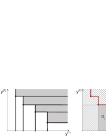
The non-dominated part of the objective space can be divided in m+1π‘š1m+1 cells. Then, given a non-dominated cell Ξ©jsubscriptΩ𝑗\Omega_{j}, only four cases arise for Ξ©isubscriptΩ𝑖\Omega_{i} (the cell of the new observation), as shown in Figure 4, for which the quantities pi​j​(𝐱)subscript𝑝𝑖𝑗𝐱p_{ij}(\mathbf{x}) need to be computed.

Refer to caption
Figure 4: Left: the m+1π‘š1m+1 non-dominated cells (in white). Right: the four cases for Ξ©isubscriptΩ𝑖\Omega_{i} given Ξ©jsubscriptΩ𝑗\Omega_{j}: three are represented by the different hatched regions, the fourth corresponds to Ξ©j=Ξ©isubscriptΩ𝑗subscriptΩ𝑖\Omega_{j}=\Omega_{i}.

Hence, the criterion can be expressed as a sum of at most (m+1)Γ—4π‘š14(m+1)\times 4 terms. As many terms can be factorized, we finally obtain:

E​E​V​(𝐱n+1)=βˆ‘j=0mβˆ«π•Ξ±j​(𝐱),𝐸𝐸𝑉subscript𝐱𝑛1superscriptsubscript𝑗0π‘šsubscript𝕏subscript𝛼𝑗𝐱EEV(\mathbf{x}_{n+1})=\sum_{j=0}^{m}\int_{\mathbb{X}}\alpha_{j}(\mathbf{x}),

with:

Ξ±0​(𝐱)subscript𝛼0𝐱\displaystyle\alpha_{0}(\mathbf{x}) =\displaystyle= [𝚽ρ(1)​(yΒ―1(1)β£βˆ—,y~1(1)β£βˆ—)βˆ’πš½Ξ½(1)​(yΒ―1(1)β£βˆ—,Ξ·(1))]delimited-[]superscriptsubscript𝚽𝜌1superscriptsubscript¯𝑦11superscriptsubscript~𝑦11superscriptsubscript𝚽𝜈1superscriptsubscript¯𝑦11superscriptπœ‚1\displaystyle\left[\boldsymbol{\Phi}_{\rho}^{(1)}\left(\bar{y}_{1}^{(1)*},\tilde{y}_{1}^{(1)*}\right)-\boldsymbol{\Phi}_{\nu}^{(1)}\left(\bar{y}_{1}^{(1)*},\eta^{(1)}\right)\right]
Γ—\displaystyle\times [Φ​(Ξ·(2))βˆ’1]+Φ​(y~1(1)β£βˆ—),delimited-[]Ξ¦superscriptπœ‚21Ξ¦superscriptsubscript~𝑦11\displaystyle\left[\Phi\left(\eta^{(2)}\right)-1\right]+\Phi\left(\tilde{y}_{1}^{(1)*}\right),
Ξ±j​(𝐱)subscript𝛼𝑗𝐱\displaystyle\alpha_{j}(\mathbf{x}) =\displaystyle= [𝚽ρ(1)(yΒ―j+1(1)β£βˆ—,y~j+1(1)β£βˆ—)βˆ’πš½Ξ½(1)(yΒ―j+1(1)β£βˆ—,Ξ·(1))\displaystyle\big{[}\boldsymbol{\Phi}_{\rho}^{(1)}\left(\bar{y}_{j+1}^{(1)*},\tilde{y}_{j+1}^{(1)*}\right)-\boldsymbol{\Phi}_{\nu}^{(1)}\left(\bar{y}_{j+1}^{(1)*},\eta^{(1)}\right)
+\displaystyle+ 𝚽ν(1)(yΒ―j(1)β£βˆ—,Ξ·(1))βˆ’πš½Ο(1)(yΒ―j(1)β£βˆ—,y~j(1)β£βˆ—)]\displaystyle\boldsymbol{\Phi}_{\nu}^{(1)}\left(\bar{y}_{j}^{(1)*},\eta^{(1)}\right)-\boldsymbol{\Phi}_{\rho}^{(1)}\left(\bar{y}_{j}^{(1)*},\tilde{y}_{j}^{(1)*}\right)\big{]}
Γ—\displaystyle\times [𝚽ν(2)​(yΒ―j(2)β£βˆ—,Ξ·(2))βˆ’πš½Ο(2)​(yΒ―j(2)β£βˆ—,yj(2)β£βˆ—)]delimited-[]superscriptsubscript𝚽𝜈2superscriptsubscript¯𝑦𝑗2superscriptπœ‚2superscriptsubscript𝚽𝜌2superscriptsubscript¯𝑦𝑗2superscriptsubscript𝑦𝑗2\displaystyle\left[\boldsymbol{\Phi}_{\nu}^{(2)}\left(\bar{y}_{j}^{(2)*},\eta^{(2)}\right)-\boldsymbol{\Phi}_{\rho}^{(2)}\left(\bar{y}_{j}^{(2)*},y_{j}^{(2)*}\right)\right]
+\displaystyle+ [Φ​(y~j+1(1)β£βˆ—)βˆ’Ξ¦β€‹(y~j(1)β£βˆ—)]​Φ​(y~j(2)β£βˆ—),delimited-[]Ξ¦superscriptsubscript~𝑦𝑗11Ξ¦superscriptsubscript~𝑦𝑗1Ξ¦superscriptsubscript~𝑦𝑗2\displaystyle\left[\Phi\left(\tilde{y}_{j+1}^{(1)*}\right)-\Phi\left(\tilde{y}_{j}^{(1)*}\right)\right]\Phi\left(\tilde{y}_{j}^{(2)*}\right),
βˆ€jfor-all𝑗\displaystyle\forall j ∈\displaystyle\in {1,…,mβˆ’1},1β€¦π‘š1\displaystyle\{1,\ldots,m-1\},

and:

Ξ±m​(𝐱)subscriptπ›Όπ‘šπ±\displaystyle\alpha_{m}(\mathbf{x}) =\displaystyle= [1βˆ’Ξ¦(Ξ·(1))+𝚽ν(1)(yΒ―m(1)β£βˆ—,Ξ·(1))\displaystyle\big{[}1-\Phi\left(\eta^{(1)}\right)+\boldsymbol{\Phi}_{\nu}^{(1)}\left(\bar{y}_{m}^{(1)*},\eta^{(1)}\right)
βˆ’\displaystyle- 𝚽ρ(1)(yΒ―m(1)β£βˆ—,y~m(1)β£βˆ—)]\displaystyle\boldsymbol{\Phi}_{\rho}^{(1)}\left(\bar{y}_{m}^{(1)*},\tilde{y}_{m}^{(1)*}\right)\big{]}
Γ—\displaystyle\times [𝚽ν(2)​(yΒ―m(2)β£βˆ—,Ξ·(2))βˆ’πš½Ο(2)​(yΒ―m(2)β£βˆ—,y~m(2)β£βˆ—)]delimited-[]superscriptsubscript𝚽𝜈2superscriptsubscriptΒ―π‘¦π‘š2superscriptπœ‚2superscriptsubscript𝚽𝜌2superscriptsubscriptΒ―π‘¦π‘š2superscriptsubscript~π‘¦π‘š2\displaystyle\left[\boldsymbol{\Phi}_{\nu}^{(2)}\left(\bar{y}_{m}^{(2)*},\eta^{(2)}\right)-\boldsymbol{\Phi}_{\rho}^{(2)}\left(\bar{y}_{m}^{(2)*},\tilde{y}_{m}^{(2)*}\right)\right]
+\displaystyle+ [1βˆ’Ξ¦β€‹(yΒ―m(1)β£βˆ—)]​Φ​(yΒ―m(2)β£βˆ—).delimited-[]1Ξ¦superscriptsubscriptΒ―π‘¦π‘š1Ξ¦superscriptsubscriptΒ―π‘¦π‘š2\displaystyle\left[1-\Phi\left(\bar{y}_{m}^{(1)*}\right)\right]\Phi\left(\bar{y}_{m}^{(2)*}\right).

Calculations are not detailed, as they are straightforward developments of Eq.Β (13). The two extremal terms (j=0𝑗0j=0 and j=m+1π‘—π‘š1j=m+1) correspond to special cases of Ξ©jsubscriptΩ𝑗\Omega_{j} (first and last cells in Figure 4, right).

5 Numerical experiments

5.1 One-dimensional, bi-objective problem

In this section, we apply the method to the following bi-objective problem: F(1)superscript𝐹1F^{(1)} and F(2)superscript𝐹2F^{(2)} are independent realizations of one-dimensional GPs, indexed by a 300-point regular grid on [0,1]01[0,1], with a stationary Matern covariance with regularity parameter ν=3/2𝜈32\nu=3/2 (Rasmussen and Williams, 2006, chapter 4). The variance and range parameters are taken as one and 1/5151/5, respectively.

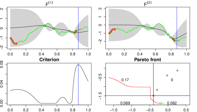
Now, two GP models are built based on four randomly chosen observations. The covariance function is considered as known. Figure 5 shows the initial models and Pareto front. Here, a single point dominates the three others. After building the tesselation as described in Section 4.1, we compute the volume of the excursion sets corresponding to each cell (Eq.Β (11)). As there are only four observations, the probability to belong to a non-dominated cell is relatively high (Figure 5, bottom right). Then, the criterion is computed for each point in the grid (Figure 5, bottom right). Its maximum is obtained in a region with high uncertainty and low expected values for the two functions.
Refer to caption
Figure 5: Top graphs: initial models (same representation as Figure 1); the actual Pareto-optimal points are represented by red crosses. Bottom right: observations (black circles) represented in the objective space, actual Pareto front (red) and current front (blue). Bottom left: criterion value as a function of 𝐱𝐱\mathbf{x}. The vertical bars show the new observation location; the green circle is the new observation.

After 10 iterations (Figure 6), the Pareto front is well-approximated. The models are accurate in the optimal regions and have high prediction variances in the other regions, which indicates a good allocation of the computational resources.

Refer to caption
Figure 6: Models and Pareto front after 10 iterations.

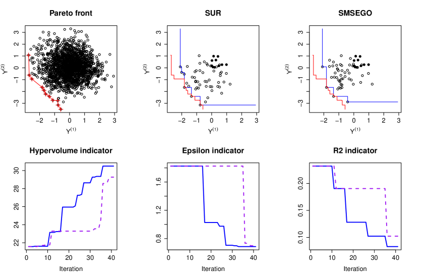
Next, we compare these results to a state-of-the-art method, called SMS-EGO (Ponweiser etΒ al., 2008), which has been shown to outperform significantly non-GP based methods (such as NSGA-II), in particular when only a limited budget of evaluation is available. As measuring performances is non-trivial in multi-criteria optimization, we use a series of three indicators: hypervolume, epsilon and R2subscript𝑅2R_{2} indicators (Zitzler etΒ al., 2003; Hansen and Jaszkiewicz, 1998), all available in the R package EMOA (Mersmann, 2012). They provide different measures of distance to the actual Pareto set and coverage of the objective space. Results are reported in Figure 7. The Pareto front obtained with SMS-EGO shows that the algorithm only detected one of the two Pareto optimal regions. As a consequence, the Pareto front is locally more accurate than the one obtained with the SUR strategy, but the indicators are much poorer.

Refer to caption
Figure 7: SMS-EGO Pareto front after 10 iterations (left) and performance comparison between SUR (plain line) and SMS-EGO (dotted line) on a one-dimensional problem. Hypervolume indicator: higher is better; other indicators should tend to zero.

5.2 Six-dimensional, bi-objective problem

Here, the objectives functions are realizations of six-dimensional GPs indexed by a 2000-point Sobol sequence on [0,1]6superscript016[0,1]^{6}, with a stationary Matern covariance with regularity parameter ν=5/2𝜈52\nu=5/2. The variance and range parameters are taken as one and 6/666\sqrt{6}/6, respectively. The initial experimental set consists of 10 points randomly chosen, and 40 points are added iteratively using the SUR and SMS-EGO strategies. The results are given in Figure 8. Again, the SUR strategy shows better performances compared to SMS-EGO.
Refer to caption
Figure 8: Performance comparison between SUR (plain line) and SMS-EGO (dotted line) on a six-dimensional problem. Top left: all 2000 points in the objective space; Pareto-optimal points are the red crosses. Top middle and right: Pareto fronts after 40 iterations.

6 Discussion

We have proposed a new sequential sampling strategy, based on stepwise uncertainty reduction principles, for multi-objective optimization. Closed-form expressions were provided for the infill criterion. Numerical experiments showed promising performances of our strategy compared to a state-of-the-art method. We point here some strengths and weaknesses of our approach.

First of all, as it is based on Gaussian process modeling, it shares the limits inherents to the model. In particular, it is well-known that classical GP models cannot cope with large datasets (>1000absent1000>1000) or high-dimensional spaces (>100absent100>100). Most models also have restrictive conditions on the approximated function (typically, stationarity), and the strategy efficiency may be greatly penalized by important inadequations between the model hypothesis and the actual function characteristics. Using the proposed strategy on more complex GP models (Gramacy and Lee, 2008; Banerjee etΒ al., 2013) may help mitigate these issues.

Secondly, we wish to emphasize here that the proposed method has a non-negligible computational cost, as (a) the criterion is evaluated by numerical integration and (b) it is embedded in an optimization loop. Hence, its use may be limited to simulators for which the time to compute an evaluation is much higher than the time to choose the next point to evaluate. However, one may note that the use of closed-form expressions, although relying on the bivariate normal CDF, avoid the need to use conditional simulations (as in Villemonteix etΒ al. (2009)) that would have made the method overly expensive.

On the other hand, moving away from the expected improvement paradigm allowed us to provide a method that does not necessitate any artificial ranking or trade-off between objective functions. It is also scale-invariant, which can be of great advantage when dealing with objectives of different nature. Finally, one advantage of the proposed strategy is that it considers progress in the design space rather than in the objective space, which corresponds to what practitioners are eventually interested in.

Possible extensions of this work are various. Accounting for the uncertainty due to the estimation of the model hyperparameters were left appart here; Bayesian approaches, in the fashion of Kennedy and O’Hagan (2001) or Gramacy and Lee (2008) for instance, may help address this issue. Objective functions were considered as not correlated to ease calculations and allow the use of simple models. As objectives are likely to be negatively correlated in practice, accounting for it while keeping tractable criteria is an important question. Finally, the stepwise uncertainty reduction strategy may be easily adapted to other frameworks, such as constrained or noisy optimization.

Appendix A Probabilities update

A.1 Proof of Proposition 3.2

Using the model update equations (4), we note first that:

pn+1​(𝐱,a)=Φ​[aβˆ’mn​(𝐱)+cn​(𝐱,𝐱n+1)sn2​(𝐱n+1)​[mn​(𝐱n+1)βˆ’yn+1]sn+1​(𝐱)]subscript𝑝𝑛1π±π‘ŽΞ¦delimited-[]π‘Žsubscriptπ‘šπ‘›π±subscript𝑐𝑛𝐱subscript𝐱𝑛1superscriptsubscript𝑠𝑛2subscript𝐱𝑛1delimited-[]subscriptπ‘šπ‘›subscript𝐱𝑛1subscript𝑦𝑛1subscript𝑠𝑛1𝐱p_{n+1}(\mathbf{x},a)=\Phi\left[\frac{a-m_{n}(\mathbf{x})+\frac{c_{n}(\mathbf{x},\mathbf{x}_{n+1})}{s_{n}^{2}(\mathbf{x}_{n+1})}\left[m_{n}\left(\mathbf{x}_{n+1}\right)-y_{n+1}\right]}{s_{n+1}(\mathbf{x})}\right]

Now, let φ​(yn+1)πœ‘subscript𝑦𝑛1\varphi\left(y_{n+1}\right) be the PDF of Yn+1subscriptπ‘Œπ‘›1Y_{n+1} (conditional on π’œnsubscriptπ’œπ‘›\mathcal{A}_{n}). We have:

q​(𝐱,b,a)=βˆ«βˆ’βˆžbpn+1​(𝐱,a)​𝑑φ​(yn+1)=βˆ«βˆ’βˆžbΦ​[aβˆ’mn​(𝐱)+cn​(𝐱,𝐱n+1)sn2​(𝐱n+1)​[mn​(𝐱n+1)βˆ’yn+1]sn+1​(𝐱)]d​φ​(yn+1)π‘žπ±π‘π‘Žsuperscriptsubscript𝑏subscript𝑝𝑛1π±π‘Ždifferential-dπœ‘subscript𝑦𝑛1superscriptsubscript𝑏Φdelimited-[]π‘Žsubscriptπ‘šπ‘›π±subscript𝑐𝑛𝐱subscript𝐱𝑛1superscriptsubscript𝑠𝑛2subscript𝐱𝑛1delimited-[]subscriptπ‘šπ‘›subscript𝐱𝑛1subscript𝑦𝑛1subscript𝑠𝑛1π±π‘‘πœ‘subscript𝑦𝑛1\begin{split}&q(\mathbf{x},b,a)\\ =&\int_{-\infty}^{b}p_{n+1}(\mathbf{x},a)d\varphi\left(y_{n+1}\right)\\ =&\int_{-\infty}^{b}\Phi\left[\frac{a-m_{n}(\mathbf{x})+\frac{c_{n}(\mathbf{x},\mathbf{x}_{n+1})}{s_{n}^{2}(\mathbf{x}_{n+1})}\left[m_{n}\left(\mathbf{x}_{n+1}\right)-y_{n+1}\right]}{s_{n+1}(\mathbf{x})}\right]\\ &d\varphi\left(y_{n+1}\right)\end{split}

As Yn+1βˆΌπ’©β€‹(mn​(𝐱n+1),sn2​(𝐱n+1))similar-tosubscriptπ‘Œπ‘›1𝒩subscriptπ‘šπ‘›subscript𝐱𝑛1superscriptsubscript𝑠𝑛2subscript𝐱𝑛1Y_{n+1}\sim\mathcal{N}\left(m_{n}(\mathbf{x}_{n+1}),s_{n}^{2}(\mathbf{x}_{n+1})\right), we can write (following Chevalier etΒ al. (2012)):

Yn+1=mn​(𝐱n+1)+sn​(𝐱n+1)​Usubscriptπ‘Œπ‘›1subscriptπ‘šπ‘›subscript𝐱𝑛1subscript𝑠𝑛subscript𝐱𝑛1π‘ˆY_{n+1}=m_{n}(\mathbf{x}_{n+1})+s_{n}(\mathbf{x}_{n+1})U

with

UβˆΌπ’©β€‹(0,1),similar-toπ‘ˆπ’©01U\sim\mathcal{N}\left(0,1\right),

which allows to simplify the previous equations to:

q​(𝐱,b,a)=βˆ«βˆ’βˆžb¯Φ​[aβˆ’mn​(𝐱)sn+1​(𝐱)βˆ’(cn​(𝐱,𝐱n+1)sn​(𝐱n+1)​sn+1​(𝐱))​u]​𝑑φ​(u)=βˆ«βˆ’βˆžb¯Φ​[a^βˆ’Ξ²β€‹u]​𝑑φ​(u),π‘žπ±π‘π‘Žsuperscriptsubscript¯𝑏Φdelimited-[]π‘Žsubscriptπ‘šπ‘›π±subscript𝑠𝑛1𝐱subscript𝑐𝑛𝐱subscript𝐱𝑛1subscript𝑠𝑛subscript𝐱𝑛1subscript𝑠𝑛1𝐱𝑒differential-dπœ‘π‘’superscriptsubscript¯𝑏Φdelimited-[]^π‘Žπ›½π‘’differential-dπœ‘π‘’\begin{split}&q(\mathbf{x},b,a)\\ &=\int_{-\infty}^{\bar{b}}\Phi\left[\frac{a-m_{n}(\mathbf{x})}{s_{n+1}(\mathbf{x})}-\left(\frac{c_{n}(\mathbf{x},\mathbf{x}_{n+1})}{s_{n}(\mathbf{x}_{n+1})s_{n+1}(\mathbf{x})}\right)u\right]d\varphi(u)\\ &=\int_{-\infty}^{\bar{b}}\Phi\left[\hat{a}-\beta u\right]d\varphi(u),\end{split} (14)

with

β𝛽\displaystyle\beta =\displaystyle= (cn​(𝐱,𝐱n+1))/(sn​(𝐱n+1)​sn+1​(𝐱)),subscript𝑐𝑛𝐱subscript𝐱𝑛1subscript𝑠𝑛subscript𝐱𝑛1subscript𝑠𝑛1𝐱\displaystyle(c_{n}(\mathbf{x},\mathbf{x}_{n+1}))/(s_{n}(\mathbf{x}_{n+1})s_{n+1}(\mathbf{x})),
a^^π‘Ž\displaystyle\hat{a} =\displaystyle= (aβˆ’mn​(𝐱))/sn+1​(𝐱)​ andπ‘Žsubscriptπ‘šπ‘›π±subscript𝑠𝑛1𝐱 and\displaystyle(a-m_{n}(\mathbf{x}))/s_{n+1}(\mathbf{x})\text{ and}
b¯¯𝑏\displaystyle\bar{b} =\displaystyle= (bβˆ’mn​(𝐱n+1))/sn​(𝐱n+1).𝑏subscriptπ‘šπ‘›subscript𝐱𝑛1subscript𝑠𝑛subscript𝐱𝑛1\displaystyle(b-m_{n}(\mathbf{x}_{n+1}))/s_{n}(\mathbf{x}_{n+1}).

This quantity can be written as a bivariate Gaussian CDF. Indeed:

βˆ«βˆ’βˆžb¯Φ​[a^βˆ’Ξ²β€‹u]​𝑑φ​(u)=12β€‹Ο€β€‹βˆ«βˆ’βˆžb¯Φ​[a^βˆ’Ξ²β€‹u]​exp⁑(βˆ’u22)​𝑑u=12β€‹Ο€β€‹βˆ«βˆ’βˆžbΒ―βˆ«βˆ’βˆža^βˆ’Ξ²β€‹uexp⁑[βˆ’12​(u2+t2)]​𝑑t​𝑑u=12β€‹Ο€β€‹βˆ«βˆ’βˆžbΒ―βˆ«βˆ’βˆža^exp⁑[βˆ’12​(u2+[tβˆ’Ξ²β€‹u]2)]​𝑑t​𝑑u=12​π​|𝚺β|β€‹βˆ«βˆ’βˆžbΒ―βˆ«βˆ’βˆža^exp⁑[βˆ’12​[ut]β€‹πšΊΞ²βˆ’1​[ut]]​𝑑t​𝑑u,superscriptsubscript¯𝑏Φdelimited-[]^π‘Žπ›½π‘’differential-dπœ‘π‘’12πœ‹superscriptsubscript¯𝑏Φdelimited-[]^π‘Žπ›½π‘’superscript𝑒22differential-d𝑒12πœ‹superscriptsubscript¯𝑏superscriptsubscript^π‘Žπ›½π‘’12superscript𝑒2superscript𝑑2differential-d𝑑differential-d𝑒12πœ‹superscriptsubscript¯𝑏superscriptsubscript^π‘Ž12superscript𝑒2superscriptdelimited-[]𝑑𝛽𝑒2differential-d𝑑differential-d𝑒12πœ‹subscriptπšΊπ›½superscriptsubscript¯𝑏superscriptsubscript^π‘Ž12delimited-[]matrix𝑒𝑑superscriptsubscriptπšΊπ›½1delimited-[]matrix𝑒𝑑differential-d𝑑differential-d𝑒\begin{split}&\int_{-\infty}^{\bar{b}}\Phi\left[\hat{a}-\beta u\right]d\varphi(u)\\ &=\frac{1}{\sqrt{2\pi}}\int_{-\infty}^{\bar{b}}\Phi\left[\hat{a}-\beta u\right]\exp\left(\frac{-u^{2}}{2}\right)du\\ &=\frac{1}{2\pi}\int_{-\infty}^{\bar{b}}\int_{-\infty}^{\hat{a}-\beta u}\exp\left[-\frac{1}{2}\left(u^{2}+t^{2}\right)\right]dtdu\\ &=\frac{1}{2\pi}\int_{-\infty}^{\bar{b}}\int_{-\infty}^{\hat{a}}\exp\left[-\frac{1}{2}\left(u^{2}+\left[t-\beta u\right]^{2}\right)\right]dtdu\\ &=\frac{1}{2\pi|\boldsymbol{\Sigma}_{\beta}|}\int_{-\infty}^{\bar{b}}\int_{-\infty}^{\hat{a}}\exp\left[-\frac{1}{2}\left[\begin{matrix}u&t\end{matrix}\right]\boldsymbol{\Sigma}_{\beta}^{-1}\left[\begin{matrix}u\\ t\end{matrix}\right]\right]dtdu,\end{split}

with 𝚺β=[1Ξ²Ξ²1+Ξ²2]subscriptπšΊπ›½delimited-[]matrix1𝛽𝛽1superscript𝛽2\boldsymbol{\Sigma}_{\beta}=\left[\begin{matrix}1&\beta\\ \beta&1+\beta^{2}\end{matrix}\right] (noting that |𝚺β|=1subscriptπšΊπ›½1|\boldsymbol{\Sigma}_{\beta}|=1), which is the standard form of the bivariate Gaussian CDF with zero mean and covariance matrix 𝚺βsubscriptπšΊπ›½\boldsymbol{\Sigma}_{\beta}, hence:

q​(𝐱,b,a)=πš½πšΊΞ²β€‹(bΒ―,a^).π‘žπ±π‘π‘Žsubscript𝚽subscriptπšΊπ›½Β―π‘^π‘Žq(\mathbf{x},b,a)=\boldsymbol{\Phi}_{\boldsymbol{\Sigma}_{\beta}}\left(\bar{b},\hat{a}\right).

Finally, applying the normalization a~=a^/1+Ξ²2~π‘Ž^π‘Ž1superscript𝛽2\tilde{a}=\hat{a}/\sqrt{1+\beta^{2}}, we have: q​(𝐱,b,a)=πš½Οβ€‹(bΒ―,a~)π‘žπ±π‘π‘Žsubscriptπš½πœŒΒ―π‘~π‘Žq(\mathbf{x},b,a)=\boldsymbol{\Phi}_{\rho}\left(\bar{b},\tilde{a}\right), with:

ρ=Ξ²1+Ξ²2=cn​(𝐱,𝐱n+1)sn​(𝐱n+1)​sn​(𝐱).πœŒπ›½1superscript𝛽2subscript𝑐𝑛𝐱subscript𝐱𝑛1subscript𝑠𝑛subscript𝐱𝑛1subscript𝑠𝑛𝐱\rho=\frac{\beta}{\sqrt{1+\beta^{2}}}=\frac{c_{n}(\mathbf{x},\mathbf{x}_{n+1})}{s_{n}(\mathbf{x}_{n+1})s_{n}(\mathbf{x})}.

A.2 Proof of Proposition 3.1

The result can be obtained directly from Proposition 3.2 with bβ†’+βˆžβ†’π‘b\rightarrow+\infty. We have then: q​(𝐱,b,a)→Φ​(a~)=pn​(𝐱,a)β†’π‘žπ±π‘π‘ŽΞ¦~π‘Žsubscriptπ‘π‘›π±π‘Žq(\mathbf{x},b,a)\rightarrow\Phi\left(\tilde{a}\right)=p_{n}(\mathbf{x},a).

A.3 Proof of Corollary 3.3

From Eq.Β (14), we have directly:

r​(𝐱,b,a)π‘Ÿπ±π‘π‘Ž\displaystyle r(\mathbf{x},b,a) =\displaystyle= ∫bΒ―+βˆžΞ¦β€‹[a^βˆ’Ξ²β€‹u]​𝑑φ​(u)superscriptsubscript¯𝑏Φdelimited-[]^π‘Žπ›½π‘’differential-dπœ‘π‘’\displaystyle\int_{\bar{b}}^{+\infty}\Phi\left[\hat{a}-\beta u\right]d\varphi(u)
=\displaystyle= βˆ«βˆ’βˆžβˆ’b¯Φ​[a^+β​u]​𝑑φ​(u)superscriptsubscript¯𝑏Φdelimited-[]^π‘Žπ›½π‘’differential-dπœ‘π‘’\displaystyle\int_{-\infty}^{-\bar{b}}\Phi\left[\hat{a}+\beta u\right]d\varphi(u)
=\displaystyle= πš½πšΊβˆ’Ξ²β€‹(βˆ’bΒ―,a^)=πš½βˆ’Οβ€‹(βˆ’bΒ―,a~).subscript𝚽subscriptπšΊπ›½Β―π‘^π‘Žsubscriptπš½πœŒΒ―π‘~π‘Ž\displaystyle\boldsymbol{\Phi}_{\boldsymbol{\Sigma}_{-\beta}}\left(-\bar{b},\hat{a}\right)=\boldsymbol{\Phi}_{-\rho}\left(-\bar{b},\tilde{a}\right).

A.4 Proof of Proposition 3.4

The steps of the proof are similar to those of Proposition 3. Using the update equations (4), we have first:

ℙ​(Y​(𝐱)≀yn+1|π’œn,yn+1=y​(𝐱n+1))=Φ​[yn+1βˆ’mn+1​(𝐱)sn+1​(𝐱)]=Φ​[βˆ’mn​(𝐱)+cn​(𝐱,𝐱n+1)​mn​(𝐱n+1)sn2​(𝐱n+1)+[1βˆ’cn​(𝐱,𝐱n+1)sn2​(𝐱n+1)]​yn+1sn+1​(𝐱)]=Φ​[mn​(𝐱n+1)βˆ’mn​(𝐱)sn+1​(𝐱)βˆ’(cn​(𝐱,𝐱n+1)βˆ’sn2​(𝐱n+1)sn​(𝐱n+1)​sn+1​(𝐱))​u].β„™π‘Œπ±conditionalsubscript𝑦𝑛1subscriptπ’œπ‘›subscript𝑦𝑛1𝑦subscript𝐱𝑛1Ξ¦delimited-[]subscript𝑦𝑛1subscriptπ‘šπ‘›1𝐱subscript𝑠𝑛1𝐱Φdelimited-[]subscriptπ‘šπ‘›π±subscript𝑐𝑛𝐱subscript𝐱𝑛1subscriptπ‘šπ‘›subscript𝐱𝑛1superscriptsubscript𝑠𝑛2subscript𝐱𝑛1delimited-[]1subscript𝑐𝑛𝐱subscript𝐱𝑛1superscriptsubscript𝑠𝑛2subscript𝐱𝑛1subscript𝑦𝑛1subscript𝑠𝑛1𝐱Φdelimited-[]subscriptπ‘šπ‘›subscript𝐱𝑛1subscriptπ‘šπ‘›π±subscript𝑠𝑛1𝐱subscript𝑐𝑛𝐱subscript𝐱𝑛1superscriptsubscript𝑠𝑛2subscript𝐱𝑛1subscript𝑠𝑛subscript𝐱𝑛1subscript𝑠𝑛1𝐱𝑒\begin{split}&\mathbb{P}\left(Y(\mathbf{x})\leq y_{n+1}|\mathcal{A}_{n},y_{n+1}=y(\mathbf{x}_{n+1})\right)\\ &=\Phi\left[\frac{y_{n+1}-m_{n+1}(\mathbf{x})}{s_{n+1}(\mathbf{x})}\right]\\ &=\Phi\left[\frac{-m_{n}(\mathbf{x})+\frac{c_{n}(\mathbf{x},\mathbf{x}_{n+1})m_{n}\left(\mathbf{x}_{n+1}\right)}{s_{n}^{2}(\mathbf{x}_{n+1})}+\left[1-\frac{c_{n}(\mathbf{x},\mathbf{x}_{n+1})}{s_{n}^{2}(\mathbf{x}_{n+1})}\right]y_{n+1}}{s_{n+1}(\mathbf{x})}\right]\\ &=\Phi\left[\frac{m_{n}(\mathbf{x}_{n+1})-m_{n}(\mathbf{x})}{s_{n+1}(\mathbf{x})}-\left(\frac{c_{n}(\mathbf{x},\mathbf{x}_{n+1})-s_{n}^{2}(\mathbf{x}_{n+1})}{s_{n}(\mathbf{x}_{n+1})s_{n+1}(\mathbf{x})}\right)u\right].\end{split}

Now:

h​(𝐱,b)=βˆ«βˆ’βˆžbℙ​(Y​(𝐱)≀Yn+1|π’œn,Yn+1=yn+1)​𝑑φ​(yn+1)=βˆ«βˆ’βˆžbΒ―Ξ¦[mn​(𝐱n+1)βˆ’mn​(𝐱)sn+1​(𝐱)βˆ’(cn​(𝐱,𝐱n+1)βˆ’sn2​(𝐱n+1)sn​(𝐱n+1)​sn+1​(𝐱))u]dΟ†(u)=βˆ«βˆ’βˆžb¯Φ​[ΞΌβˆ’Ο„β€‹u]​𝑑φ​(u)=πš½πšΊΟ„β€‹(bΒ―,ΞΌ),β„Žπ±π‘superscriptsubscriptπ‘β„™π‘Œπ±conditionalsubscriptπ‘Œπ‘›1subscriptπ’œπ‘›subscriptπ‘Œπ‘›1subscript𝑦𝑛1differential-dπœ‘subscript𝑦𝑛1superscriptsubscript¯𝑏Φdelimited-[]subscriptπ‘šπ‘›subscript𝐱𝑛1subscriptπ‘šπ‘›π±subscript𝑠𝑛1𝐱subscript𝑐𝑛𝐱subscript𝐱𝑛1superscriptsubscript𝑠𝑛2subscript𝐱𝑛1subscript𝑠𝑛subscript𝐱𝑛1subscript𝑠𝑛1π±π‘’π‘‘πœ‘π‘’superscriptsubscript¯𝑏Φdelimited-[]πœ‡πœπ‘’differential-dπœ‘π‘’subscript𝚽subscriptπšΊπœΒ―π‘πœ‡\begin{split}&h(\mathbf{x},b)\\ &=\int_{-\infty}^{b}\mathbb{P}\left(Y(\mathbf{x})\leq Y_{n+1}|\mathcal{A}_{n},Y_{n+1}=y_{n+1}\right)d\varphi\left(y_{n+1}\right)\\ &=\int_{-\infty}^{\bar{b}}\Phi\Big{[}\frac{m_{n}(\mathbf{x}_{n+1})-m_{n}(\mathbf{x})}{s_{n+1}(\mathbf{x})}\\ &-\left(\frac{c_{n}(\mathbf{x},\mathbf{x}_{n+1})-s_{n}^{2}(\mathbf{x}_{n+1})}{s_{n}(\mathbf{x}_{n+1})s_{n+1}(\mathbf{x})}\right)u\Big{]}d\varphi(u)\\ &=\int_{-\infty}^{\bar{b}}\Phi\left[\mu-\tau u\right]d\varphi(u)\\ &=\boldsymbol{\Phi}_{\boldsymbol{\Sigma}_{\tau}}\left(\bar{b},\mu\right),\end{split}

as we get a form similar to Equation 14, with πš½πšΊΟ„subscript𝚽subscript𝚺𝜏\boldsymbol{\Phi}_{\boldsymbol{\Sigma}_{\tau}} the CDF of the centered bigaussian with covariance πšΊΟ„=[1ττ1+Ο„2]subscript𝚺𝜏delimited-[]matrix1𝜏𝜏1superscript𝜏2\boldsymbol{\Sigma}_{\tau}=\left[\begin{matrix}1&\tau\\ \tau&1+\tau^{2}\end{matrix}\right],

ΞΌπœ‡\displaystyle\mu =\displaystyle= (mn​(𝐱n+1)βˆ’mn​(𝐱))/sn+1​(𝐱)subscriptπ‘šπ‘›subscript𝐱𝑛1subscriptπ‘šπ‘›π±subscript𝑠𝑛1𝐱\displaystyle(m_{n}(\mathbf{x}_{n+1})-m_{n}(\mathbf{x}))/s_{n+1}(\mathbf{x})
Ο„πœ\displaystyle\tau =\displaystyle= (cn​(𝐱,𝐱n+1)βˆ’sn2​(𝐱n+1))/(sn​(𝐱n+1)​sn+1​(𝐱)).subscript𝑐𝑛𝐱subscript𝐱𝑛1superscriptsubscript𝑠𝑛2subscript𝐱𝑛1subscript𝑠𝑛subscript𝐱𝑛1subscript𝑠𝑛1𝐱\displaystyle(c_{n}(\mathbf{x},\mathbf{x}_{n+1})-s_{n}^{2}(\mathbf{x}_{n+1}))/(s_{n}(\mathbf{x}_{n+1})s_{n+1}(\mathbf{x})).

Normalizing Ξ·=ΞΌ/1+Ο„2πœ‚πœ‡1superscript𝜏2\eta=\mu/\sqrt{1+\tau^{2}} delivers the final result.

Appendix B bi​j(k)​(𝐱)superscriptsubscriptπ‘π‘–π‘—π‘˜π±b_{ij}^{(k)}(\mathbf{x}) and di​j(k)​(𝐱)superscriptsubscriptπ‘‘π‘–π‘—π‘˜π±d_{ij}^{(k)}(\mathbf{x}) computation

Let X𝑋X and Yπ‘ŒY be two dependent random variables, and aπ‘Ža, b𝑏b, c𝑐c and d𝑑d four real numbers. By direct application of Bayes formula, we have:

ℙ​(a≀X​<b|​c≀Y<d)​ℙ​(c≀Y<d)=ℙ​(Y<d)Γ—[ℙ​(X​<b|​Y<d)βˆ’β„™β€‹(X≀a|Y<d)]βˆ’β„™β€‹(Y≀c)Γ—[ℙ​(X​<b|​Y≀c)βˆ’β„™β€‹(X≀a|Y≀c)]ℙ​(Y≀X​<b|​a≀Y<b)​ℙ​(a≀Y<b)=ℙ​(Y<b)Γ—[ℙ​(X​<b|​Y<b)βˆ’β„™β€‹(X≀Y|Y<b)]βˆ’β„™β€‹(Y≀a)Γ—[ℙ​(X​<b|​Y≀a)βˆ’β„™β€‹(X≀Y|Y≀a)]β„™π‘Žπ‘‹braπ‘π‘π‘Œπ‘‘β„™π‘π‘Œπ‘‘β„™π‘Œπ‘‘delimited-[]ℙ𝑋braπ‘π‘Œπ‘‘β„™π‘‹conditionalπ‘Žπ‘Œπ‘‘β„™π‘Œπ‘delimited-[]ℙ𝑋braπ‘π‘Œπ‘β„™π‘‹conditionalπ‘Žπ‘Œπ‘β„™π‘Œπ‘‹braπ‘π‘Žπ‘Œπ‘β„™π‘Žπ‘Œπ‘β„™π‘Œπ‘delimited-[]ℙ𝑋braπ‘π‘Œπ‘β„™π‘‹conditionalπ‘Œπ‘Œπ‘β„™π‘Œπ‘Ždelimited-[]ℙ𝑋braπ‘π‘Œπ‘Žβ„™π‘‹conditionalπ‘Œπ‘Œπ‘Ž\begin{split}&\mathbb{P}\left(a\leq X<b|c\leq Y<d\right)\mathbb{P}\left(c\leq Y<d\right)\\ &=\mathbb{P}\left(Y<d\right)\times\left[\mathbb{P}\left(X<b|Y<d\right)-\mathbb{P}\left(X\leq a|Y<d\right)\right]\\ &-\mathbb{P}\left(Y\leq c\right)\times\left[\mathbb{P}\left(X<b|Y\leq c\right)-\mathbb{P}\left(X\leq a|Y\leq c\right)\right]\\ \\ &\mathbb{P}\left(Y\leq X<b|a\leq Y<b\right)\mathbb{P}\left(a\leq Y<b\right)\\ &=\mathbb{P}\left(Y<b\right)\times\left[\mathbb{P}\left(X<b|Y<b\right)-\mathbb{P}\left(X\leq Y|Y<b\right)\right]\\ &-\mathbb{P}\left(Y\leq a\right)\times\left[\mathbb{P}\left(X<b|Y\leq a\right)-\mathbb{P}\left(X\leq Y|Y\leq a\right)\right]\end{split}

Now, by definition, bi​j(k)superscriptsubscriptπ‘π‘–π‘—π‘˜b_{ij}^{(k)} is of the form of the fist equation:

bi​j(k)​(𝐱)superscriptsubscriptπ‘π‘–π‘—π‘˜π±\displaystyle b_{ij}^{(k)}(\mathbf{x}) :=assign\displaystyle:= β„™n+1​(yjβˆ’(k)≀Y(k)​(𝐱)​<yj+(k)|​yiβˆ’(k)≀Yn+1(k)<yi+(k))subscriptℙ𝑛1subscriptsuperscriptπ‘¦π‘˜limit-from𝑗superscriptπ‘Œπ‘˜π±brasubscriptsuperscriptπ‘¦π‘˜limit-from𝑗subscriptsuperscriptπ‘¦π‘˜limit-from𝑖superscriptsubscriptπ‘Œπ‘›1π‘˜subscriptsuperscriptπ‘¦π‘˜limit-from𝑖\displaystyle{\mathbb{P}}_{n+1}\left(y^{(k)}_{j-}\leq Y^{(k)}(\mathbf{x})<y^{(k)}_{j+}|y^{(k)}_{i-}\leq Y_{n+1}^{(k)}<y^{(k)}_{i+}\right)
Γ—\displaystyle\times β„™n​[yiβˆ’(k)≀Yn+1(k)<yi+(k)],subscriptℙ𝑛delimited-[]subscriptsuperscriptπ‘¦π‘˜limit-from𝑖superscriptsubscriptπ‘Œπ‘›1π‘˜subscriptsuperscriptπ‘¦π‘˜limit-from𝑖\displaystyle{\mathbb{P}}_{n}\left[y^{(k)}_{i-}\leq Y_{n+1}^{(k)}<y^{(k)}_{i+}\right],

hence write as the sum of four terms:

bi​j(k)​(𝐱)superscriptsubscriptπ‘π‘–π‘—π‘˜π±\displaystyle b_{ij}^{(k)}(\mathbf{x}) =\displaystyle= pn(k)(𝐱n+1,yi+(k))(β„™n+1[Y(k)(𝐱)≀yj+(k)|Yn+1(k)≀yi+(k)]\displaystyle p_{n}^{(k)}(\mathbf{x}_{n+1},y^{(k)}_{i+})\Big{(}{\mathbb{P}}_{n+1}\big{[}Y^{(k)}(\mathbf{x})\leq y^{(k)}_{j+}\big{|}Y_{n+1}^{(k)}\leq y^{(k)}_{i+}\big{]}
βˆ’\displaystyle- β„™n+1[Y(k)(𝐱)≀yjβˆ’(k)|Yn+1(k)≀yi+(k)])\displaystyle{\mathbb{P}}_{n+1}\big{[}Y^{(k)}(\mathbf{x})\leq y^{(k)}_{j-}\big{|}Y_{n+1}^{(k)}\leq y^{(k)}_{i+}\big{]}\Big{)}
βˆ’\displaystyle- pn(k)(𝐱n+1,yiβˆ’(k))(β„™n+1[Y(k)(𝐱)<yj+(k)|Yn+1(k)≀yiβˆ’(k)]\displaystyle p_{n}^{(k)}(\mathbf{x}_{n+1},y^{(k)}_{i-})\Big{(}{\mathbb{P}}_{n+1}\big{[}Y^{(k)}(\mathbf{x})<y^{(k)}_{j+}\big{|}Y_{n+1}^{(k)}\leq y^{(k)}_{i-}\big{]}
βˆ’\displaystyle- β„™n+1[Y(k)(𝐱)≀yjβˆ’(k)|Yn+1(k)≀yiβˆ’(k)])\displaystyle{\mathbb{P}}_{n+1}\big{[}Y^{(k)}(\mathbf{x})\leq y^{(k)}_{j-}\big{|}Y_{n+1}^{(k)}\leq y^{(k)}_{i-}\big{]}\Big{)}
=\displaystyle= q(k)​(𝐱,yi+(k),yj+(k))βˆ’q(k)​(𝐱,yi+(k),yjβˆ’(k))superscriptπ‘žπ‘˜π±subscriptsuperscriptπ‘¦π‘˜limit-from𝑖subscriptsuperscriptπ‘¦π‘˜limit-from𝑗superscriptπ‘žπ‘˜π±subscriptsuperscriptπ‘¦π‘˜limit-from𝑖subscriptsuperscriptπ‘¦π‘˜limit-from𝑗\displaystyle q^{(k)}\left(\mathbf{x},y^{(k)}_{i+},y^{(k)}_{j+}\right)-q^{(k)}\left(\mathbf{x},y^{(k)}_{i+},y^{(k)}_{j-}\right)
βˆ’\displaystyle- q(k)​(𝐱,yiβˆ’(k),yj+(k))+q(k)​(𝐱,yiβˆ’(k),yjβˆ’(k)),superscriptπ‘žπ‘˜π±subscriptsuperscriptπ‘¦π‘˜limit-from𝑖subscriptsuperscriptπ‘¦π‘˜limit-from𝑗superscriptπ‘žπ‘˜π±subscriptsuperscriptπ‘¦π‘˜limit-from𝑖subscriptsuperscriptπ‘¦π‘˜limit-from𝑗\displaystyle q^{(k)}\left(\mathbf{x},y^{(k)}_{i-},y^{(k)}_{j+}\right)+q^{(k)}\left(\mathbf{x},y^{(k)}_{i-},y^{(k)}_{j-}\right),

with q(k)​(𝐱,b,a)superscriptπ‘žπ‘˜π±π‘π‘Žq^{(k)}(\mathbf{x},b,a) given by Eq.Β (5), thus:

bi​j(k)​(𝐱)superscriptsubscriptπ‘π‘–π‘—π‘˜π±\displaystyle b_{ij}^{(k)}(\mathbf{x}) =\displaystyle= 𝚽ρ(k)​(yΒ―i+(k),y~j+(k))βˆ’πš½Ο(k)​(yΒ―i+(k),y~jβˆ’(k))superscriptsubscriptπš½πœŒπ‘˜subscriptsuperscriptΒ―π‘¦π‘˜limit-from𝑖subscriptsuperscript~π‘¦π‘˜limit-from𝑗superscriptsubscriptπš½πœŒπ‘˜subscriptsuperscriptΒ―π‘¦π‘˜limit-from𝑖subscriptsuperscript~π‘¦π‘˜limit-from𝑗\displaystyle\boldsymbol{\Phi}_{\rho}^{(k)}\left(\overline{y}^{(k)}_{i+},\widetilde{y}^{(k)}_{j+}\right)-\boldsymbol{\Phi}_{\rho}^{(k)}\left(\overline{y}^{(k)}_{i+},\widetilde{y}^{(k)}_{j-}\right)
βˆ’πš½Ο(k)​(yΒ―iβˆ’(k),y~j+(k))+𝚽ρ(k)​(yΒ―iβˆ’(k),y~jβˆ’(k)).superscriptsubscriptπš½πœŒπ‘˜subscriptsuperscriptΒ―π‘¦π‘˜limit-from𝑖subscriptsuperscript~π‘¦π‘˜limit-from𝑗superscriptsubscriptπš½πœŒπ‘˜subscriptsuperscriptΒ―π‘¦π‘˜limit-from𝑖subscriptsuperscript~π‘¦π‘˜limit-from𝑗\displaystyle-\boldsymbol{\Phi}_{\rho}^{(k)}\left(\overline{y}^{(k)}_{i-},\widetilde{y}^{(k)}_{j+}\right)+\boldsymbol{\Phi}_{\rho}^{(k)}\left(\overline{y}^{(k)}_{i-},\widetilde{y}^{(k)}_{j-}\right).

Similary, di​j(k)superscriptsubscriptπ‘‘π‘–π‘—π‘˜d_{ij}^{(k)} is of the form of the second equation: Starting with the definition:

di​j(k)​(𝐱)superscriptsubscriptπ‘‘π‘–π‘—π‘˜π±\displaystyle d_{ij}^{(k)}(\mathbf{x}) :=assign\displaystyle:= β„™n+1​(Yn+1(k)≀Y(k)​(𝐱)​<yj+(k)|​yiβˆ’(k)≀Yn+1(k)<yi+(k))subscriptℙ𝑛1superscriptsubscriptπ‘Œπ‘›1π‘˜superscriptπ‘Œπ‘˜π±brasubscriptsuperscriptπ‘¦π‘˜limit-from𝑗subscriptsuperscriptπ‘¦π‘˜limit-from𝑖superscriptsubscriptπ‘Œπ‘›1π‘˜subscriptsuperscriptπ‘¦π‘˜limit-from𝑖\displaystyle{\mathbb{P}}_{n+1}\left(Y_{n+1}^{(k)}\leq Y^{(k)}(\mathbf{x})<y^{(k)}_{j+}\big{|}y^{(k)}_{i-}\leq Y_{n+1}^{(k)}<y^{(k)}_{i+}\right)
Γ—\displaystyle\times β„™n​[yiβˆ’(k)≀Yn+1(k)<yi+(k)],subscriptℙ𝑛delimited-[]subscriptsuperscriptπ‘¦π‘˜limit-from𝑖superscriptsubscriptπ‘Œπ‘›1π‘˜subscriptsuperscriptπ‘¦π‘˜limit-from𝑖\displaystyle{\mathbb{P}}_{n}\left[y^{(k)}_{i-}\leq Y_{n+1}^{(k)}<y^{(k)}_{i+}\right],

hence writes:

di​j(k)​(𝐱)superscriptsubscriptπ‘‘π‘–π‘—π‘˜π±\displaystyle d_{ij}^{(k)}(\mathbf{x}) =\displaystyle= pn(k)(𝐱n+1,yi+(k))(β„™n+1[Y(k)(𝐱)≀yj+(k)|Yn+1(k)≀yi+(k)]\displaystyle p_{n}^{(k)}(\mathbf{x}_{n+1},y^{(k)}_{i+})\Big{(}{\mathbb{P}}_{n+1}\big{[}Y^{(k)}(\mathbf{x})\leq y^{(k)}_{j+}\big{|}Y_{n+1}^{(k)}\leq y^{(k)}_{i+}\big{]}
βˆ’\displaystyle- β„™n+1[Y(k)(𝐱)≀Yn+1(k)|Yn+1(k)≀yi+(k)])\displaystyle{\mathbb{P}}_{n+1}\big{[}Y^{(k)}(\mathbf{x})\leq Y_{n+1}^{(k)}\big{|}Y_{n+1}^{(k)}\leq y^{(k)}_{i+}\big{]}\Big{)}
βˆ’\displaystyle- pn(k)(𝐱n+1,yiβˆ’(k))(β„™n+1[Y(k)(𝐱)<yj+(k)|Yn+1(k)≀yiβˆ’(k)]\displaystyle p_{n}^{(k)}(\mathbf{x}_{n+1},y^{(k)}_{i-})\Big{(}{\mathbb{P}}_{n+1}\big{[}Y^{(k)}(\mathbf{x})<y^{(k)}_{j+}\big{|}Y_{n+1}^{(k)}\leq y^{(k)}_{i-}\big{]}
βˆ’\displaystyle- β„™n+1[Y(k)(𝐱)≀Yn+1(k)|Yn+1(k)≀yiβˆ’(k)])\displaystyle{\mathbb{P}}_{n+1}\big{[}Y^{(k)}(\mathbf{x})\leq Y_{n+1}^{(k)}\big{|}Y_{n+1}^{(k)}\leq y^{(k)}_{i-}\big{]}\Big{)}
=\displaystyle= q(k)​(𝐱,yi+(k),yj+(k))βˆ’h(k)​(𝐱,yi+(k))superscriptπ‘žπ‘˜π±subscriptsuperscriptπ‘¦π‘˜limit-from𝑖subscriptsuperscriptπ‘¦π‘˜limit-from𝑗superscriptβ„Žπ‘˜π±subscriptsuperscriptπ‘¦π‘˜limit-from𝑖\displaystyle q^{(k)}\left(\mathbf{x},y^{(k)}_{i+},y^{(k)}_{j+}\right)-h^{(k)}\left(\mathbf{x},y^{(k)}_{i+}\right)
βˆ’\displaystyle- h(k)​(𝐱,yiβˆ’(k))+q(k)​(𝐱,yiβˆ’(k),yjβˆ’(k)),superscriptβ„Žπ‘˜π±subscriptsuperscriptπ‘¦π‘˜limit-from𝑖superscriptπ‘žπ‘˜π±subscriptsuperscriptπ‘¦π‘˜limit-from𝑖subscriptsuperscriptπ‘¦π‘˜limit-from𝑗\displaystyle h^{(k)}\left(\mathbf{x},y^{(k)}_{i-}\right)+q^{(k)}\left(\mathbf{x},y^{(k)}_{i-},y^{(k)}_{j-}\right),

with q(k)​(𝐱,b,a)superscriptπ‘žπ‘˜π±π‘π‘Žq^{(k)}(\mathbf{x},b,a) given by Eq.Β (5) and h(k)​(𝐱,b)superscriptβ„Žπ‘˜π±π‘h^{(k)}\left(\mathbf{x},b\right) given by Eq.Β (7), thus:

di​j(k)​(𝐱)superscriptsubscriptπ‘‘π‘–π‘—π‘˜π±\displaystyle d_{ij}^{(k)}(\mathbf{x}) =\displaystyle= 𝚽ρ(k)​(yΒ―i+(k),y~j+(k))βˆ’πš½Ξ½(k)​(yΒ―i+(k),Ξ·(k))superscriptsubscriptπš½πœŒπ‘˜subscriptsuperscriptΒ―π‘¦π‘˜limit-from𝑖subscriptsuperscript~π‘¦π‘˜limit-from𝑗superscriptsubscriptπš½πœˆπ‘˜subscriptsuperscriptΒ―π‘¦π‘˜limit-from𝑖superscriptπœ‚π‘˜\displaystyle\boldsymbol{\Phi}_{\rho}^{(k)}\left(\overline{y}^{(k)}_{i+},\widetilde{y}^{(k)}_{j+}\right)-\boldsymbol{\Phi}_{\nu}^{(k)}\left(\overline{y}^{(k)}_{i+},\eta^{(k)}\right)
+\displaystyle+ 𝚽ν(k)​(yΒ―iβˆ’(k),Ξ·(k))βˆ’πš½Ο(k)​(yΒ―iβˆ’(k),y~j+(k)).superscriptsubscriptπš½πœˆπ‘˜subscriptsuperscriptΒ―π‘¦π‘˜limit-from𝑖superscriptπœ‚π‘˜superscriptsubscriptπš½πœŒπ‘˜subscriptsuperscriptΒ―π‘¦π‘˜limit-from𝑖subscriptsuperscript~π‘¦π‘˜limit-from𝑗\displaystyle\boldsymbol{\Phi}_{\nu}^{(k)}\left(\overline{y}^{(k)}_{i-},\eta^{(k)}\right)-\boldsymbol{\Phi}_{\rho}^{(k)}\left(\overline{y}^{(k)}_{i-},\widetilde{y}^{(k)}_{j+}\right).

References

  • Banerjee etΒ al. (2013) Banerjee, A., Dunson, D.B., Tokdar, S.T.: Efficient gaussian process regression for large datasets. Biometrika 100(1), 75–89 (2013)
  • Bect etΒ al. (2012) Bect, J., Ginsbourger, D., Li, L., Picheny, V., Vazquez, E.: Sequential design of computer experiments for the estimation of a probability of failure. Statistics and Computing 22(3), 773–793 (2012)
  • Chevalier etΒ al. (2012) Chevalier, C., Bect, J., Ginsbourger, D., Vazquez, E., Picheny, V., Richet, Y.: Fast parallel kriging-based stepwise uncertainty reduction with application to the identification of an excursion set. http://hal.inria.fr/hal-00641108/en (2012)
  • Chevalier etΒ al. (2013) Chevalier, C., Picheny, V., Ginsbourger, D.: Kriginv: An efficient and user-friendly implementation of batch-sequential inversion strategies based on kriging. Computational Statistics & Data Analysis (2013)
  • Collette and Siarry (2003) Collette, Y., Siarry, P.: Multiobjective optimization: principles and case studies. Springer (2003)
  • Craig etΒ al. (2001) Craig, P.S., Goldstein, M., Rougier, J.C., Seheult, A.H.: Bayesian forecasting for complex systems using computer simulators. Journal of the American Statistical Association 96(454), 717–729 (2001)
  • Cressie (1993) Cressie, N.: Statistics for Spatial Data, revised edition, vol. 928. Wiley, New York (1993)
  • Emery (2009) Emery, X.: The kriging update equations and their application to the selection of neighboring data. Computational Geosciences 13(3), 269–280 (2009)
  • Gramacy and Lee (2011) Gramacy, L., Lee, H.: Optimization under unknown constraints. Bayesian Statistics 9, 229 (2011)
  • Gramacy and Lee (2008) Gramacy, R.B., Lee, H.K.: Bayesian treed gaussian process models with an application to computer modeling. Journal of the American Statistical Association 103(483) (2008)
  • Hansen and Jaszkiewicz (1998) Hansen, M.P., Jaszkiewicz, A.: Evaluating the quality of approximations to the non-dominated set. IMM, Department of Mathematical Modelling, Technical University of Denmark (1998)
  • Jones (2001) Jones, D.R.: A taxonomy of global optimization methods based on response surfaces. Journal of global optimization 21(4), 345–383 (2001)
  • Jones etΒ al. (1998) Jones, D.R., Schonlau, M., Welch, W.J.: Efficient global optimization of expensive black-box functions. Journal of Global optimization 13(4), 455–492 (1998)
  • Keane (2006) Keane, A.J.: Statistical improvement criteria for use in multiobjective design optimization. AIAA journal 44(4), 879–891 (2006)
  • Kenkel (2012) Kenkel, B.: pbivnorm: Vectorized Bivariate Normal CDF (2012). URL http://CRAN.R-project.org/package=pbivnorm. R package version 0.5-1
  • Kennedy and O’Hagan (2001) Kennedy, M.C., O’Hagan, A.: Bayesian calibration of computer models. Journal of the Royal Statistical Society: Series B (Statistical Methodology) 63(3), 425–464 (2001)
  • Knowles (2006) Knowles, J.: Parego: A hybrid algorithm with on-line landscape approximation for expensive multiobjective optimization problems. Evolutionary Computation, IEEE Transactions on 10(1), 50–66 (2006)
  • Mersmann (2012) Mersmann, O.: emoa: Evolutionary Multiobjective Optimization Algorithms (2012). URL http://CRAN.R-project.org/package=emoa. R package version 0.5-0
  • Ponweiser etΒ al. (2008) Ponweiser, W., Wagner, T., Biermann, D., Vincze, M.: Multiobjective optimization on a limited budget of evaluations using model-assisted s-metric selection. In: Parallel Problem Solving from Nature, pp. 784–794. Springer (2008)
  • Rasmussen and Williams (2006) Rasmussen, C., Williams, C.: Gaussian processes for machine learning. MIT Press (2006)
  • Roustant etΒ al. (2012) Roustant, O., Ginsbourger, D., Deville, Y.: Dicekriging, diceoptim: Two r packages for the analysis of computer experiments by kriging-based metamodeling and optimization. Journal of Statistical Software 51(1), 1–55 (2012)
  • Scott etΒ al. (2011) Scott, W., Frazier, P., Powell, W.: The correlated knowledge gradient for simulation optimization of continuous parameters using gaussian process regression. SIAM Journal on Optimization 21(3), 996–1026 (2011)
  • Stein (1999) Stein, M.: Interpolation of spatial data: some theory for kriging. Springer Verlag (1999)
  • Villemonteix etΒ al. (2009) Villemonteix, J., Vazquez, E., Walter, E.: An informational approach to the global optimization of expensive-to-evaluate functions. Journal of Global Optimization 44(4), 509–534 (2009)
  • Wagner etΒ al. (2010) Wagner, T., Emmerich, M., Deutz, A., Ponweiser, W.: On expected-improvement criteria for model-based multi-objective optimization. In: Parallel Problem Solving from Nature, PPSN XI, pp. 718–727. Springer (2010)
  • Wang and Shan (2007) Wang, G.G., Shan, S.: Review of metamodeling techniques in support of engineering design optimization. Journal of Mechanical Design 129, 370 (2007)
  • Zitzler etΒ al. (2003) Zitzler, E., Thiele, L., Laumanns, M., Fonseca, C.M., DaΒ Fonseca, V.G.: Performance assessment of multiobjective optimizers: An analysis and review. Evolutionary Computation, IEEE Transactions on 7(2), 117–132 (2003)