Characterizing SASI- and Convection-Dominated Core-Collapse Supernova Explosions in Two Dimensions
Abstract
The success of the neutrino mechanism of core-collapse supernovae relies on the supporting action of two hydrodynamic instabilities: neutrino-driven convection and the Standing Accretion Shock Instability (SASI). Depending on the structure of the stellar progenitor, each of these instabilities can dominate the evolution of the gain region prior to the onset of explosion, with implications for the ensuing asymmetries. Here we examine the flow dynamics in the neighborhood of explosion by means of parametric two-dimensional, time-dependent hydrodynamic simulations for which the linear stability properties are well understood. We find that systems for which the convection parameter is sub-critical (SASI-dominated) develop explosions once large-scale, high-entropy bubbles are able to survive for several SASI oscillation cycles. These long-lived structures are seeded by the SASI during shock expansions. Finite-amplitude initial perturbations do not alter this outcome qualitatively, though they can lead to significant differences in explosion times. Supercritical systems (convection-dominated) also explode by developing large-scale bubbles, though the formation of these structures is due to buoyant activity. Non-exploding systems achieve a quasi-steady state in which the time-averaged flow adjusts itself to be convectively sub-critical. We characterize the turbulent flow using a spherical Fourier-Bessel decomposition, identifying the relevant scalings and connecting temporal and spatial components. Finally, we verify the applicability of these principles on the general relativistic, radiation-hydrodynamic simulations of Müller, Janka, & Heger (2012), and discuss implications for the three-dimensional case.
keywords:
hydrodynamics — instabilities – neutrinos – nuclear reactions, nucleosynthesis, abundances — shock waves – supernovae: general1 Introduction
In the neutrino mechanism of core-collapse supernovae, a small fraction of the energy emitted in neutrinos by the forming neutron star is deposited in a layer behind the stalled accretion shock, powering its final expansion (Bethe & Wilson, 1985). Extensive theoretical work over the last two decades has led to a consensus on the failure of this mechanism in spherically symmetric systems, except for the very lightest stellar progenitors (see, e.g., Janka 2012 for a recent review).
Successful neutrino-driven explosions require additional assistance by non-spherical hydrodynamic instabilities that increase the efficiency of neutrino energy deposition. This phenomenon has been observed in numerous two-dimensional (e.g., Herant et al. 1994; Burrows et al. 1995; Janka & Müller 1996; Mezzacappa et al. 1998; Scheck et al. 2006; Ohnishi et al. 2006; Buras et al. 2006; Burrows et al. 2007; Murphy & Burrows 2008; Ott et al. 2008; Marek & Janka 2009; Suwa et al. 2010; Müller et al. 2012; Couch 2013b) as well as three-dimensional (e.g., Iwakami et al. 2008; Nordhaus et al. 2010; Hanke et al. 2012; Burrows et al. 2012; Müller et al. 2012; Takiwaki et al. 2012; Ott et al. 2013; Couch 2013a; Dolence et al. 2013; Hanke et al. 2013) core-collapse simulations of various levels of sophistication. In addition to assisting the onset of explosion, these instabilities can contribute to the generation of pulsar kicks (Scheck et al., 2006; Nordhaus et al., 2010; Wongwathanarat et al., 2010), the spin-up of the forming neutron star (Fryer & Young, 2007; Blondin & Mezzacappa, 2007; Blondin & Shaw, 2007; Fernández, 2010) and the seeding of late-time asymmetries (Kifonidis et al., 2006; Hammer et al., 2010; Wongwathanarat et al., 2013).
The shock-neutrinosphere cavity is unstable to convection driven by the energy deposition from neutrinos emitted in deeper layers (e.g., Bethe 1990). This process generates kinetic energy on spatial scales comparable to or smaller than the size of the neutrino heating region. Work by Blondin et al. (2003) and Blondin & Mezzacappa (2006) isolated a distinct, global oscillatory instability of the standing accretion shock that operates independent of neutrino heating, the so-called Standing Accretion Shock Instability (SASI). The driving mechanism involves an unstable cycle of advected and acoustic perturbations trapped within the shock-neutrinosphere cavity (Foglizzo et al. 2007; Foglizzo 2009; Guilet & Foglizzo 2012). The most unstable modes of the SASI reside on the largest spatial scales. Convection and the SASI are easily distinguishable in the linear regime, but their effects become intertwined in the non-linear turbulent flow that follows the stalling of the bounce supernova shock (e.g., Scheck et al. 2008).
Recent three-dimensional studies of core-collapse supernova hydrodynamics have found that large-scale oscillation modes of the shock attain smaller amplitudes than in two dimensions (Nordhaus et al., 2010; Wongwathanarat et al., 2010; Hanke et al., 2012; Takiwaki et al., 2012; Murphy et al., 2013). This has been interpreted as a consequence of the different behavior of turbulence in two- and three-dimensions (Hanke et al., 2012), and has led to the suggestion that the SASI may play a secondary role in the explosion mechanism, if it arises at all (Burrows et al., 2012; Burrows, 2013). These models have largely focused on a small sample of stellar progenitors, however, and in many cases do not include physical effects that are favorable for the growth of the SASI (Janka et al., 2012).
Müller et al. (2012) followed the collapse and bounce of and progenitors using a two-dimensional, general relativistic hydrodynamic code with energy dependent neutrino transport, finding that differences in progenitor structure lead to very different paths to explosion. In particular, the progenitor evolution is such that the SASI dominates the dynamics throughout the pre-explosion phase. Three-dimensional simulations of the same progenitor, with similar neutrino treatment, display episodic SASI activity, though a successful explosion is not yet obtained (Hanke et al., 2013). Ott et al. (2013) evolved the same progenitor with a more approximate neutrino prescription and a higher level of numerical perturbations, initially finding smaller SASI amplitudes than Müller et al. (2012) and Hanke et al. (2013), though later confirming SASI activity (C. Ott 2013, private communication). The lack of the same level of numerical perturbations in the Müller et al. (2012) models could mean that convection dominance instead of SASI dominance is dependent not only on the progenitor structure, but also on the details of the initial conditions.
It is the purpose of this paper to investigate some of these issues involving the interplay of SASI and convection, and the implications for successful explosions. In particular, we address the following questions: (1) Is there a fundamental difference between the transition to explosion in SASI- and convection-dominated models? (2) Can finite amplitude perturbations, generated in, e.g., multi-dimensional stellar progenitors (e.g., Arnett & Meakin 2011), tilt the balance in favor of convection in situations that would otherwise be SASI-dominated? (3) Does the SASI play any discernible role in convection-dominated systems? (4) Are there systematic trends in models close to an explosion that shed insight into the operation of each instability?
Our approach is experimental, employing hydrodynamic simulations that model neutrino source terms, the equation of state, and gravity in a parametric way (e.g., Fernández & Thompson 2009a). This setup has the advantage that its linear stability properties are well understood (Fernández & Thompson, 2009b), allowing the development of model sequences that probe different parameter regimes. Our experimental approach to studying SASI and convection follows similar works (Foglizzo et al., 2006; Ohnishi et al., 2006; Scheck et al., 2008; Fernández & Thompson, 2009a; Burrows et al., 2012), to which we relate our findings. To connect with more realistic models, we also test the generality of our analysis results on the simulations of Müller et al. (2012).
The structure of the paper is the following. Section 2 describes the numerical models employed and introduces the Spherical Fourier-Bessel decomposition. Section 3 presents results, separated by exploding and quasi-steady state behavior. A summary and discussion follows in Section 4. Appendix A addresses the stability of the mode in the parametric setup, and Appendix B provides details about the spherical basis functions for the cases of Dirichlet and Neumann boundary conditions.
2 Methods
2.1 Parametric Hydrodynamic Simulations
2.1.1 Numerical Setup
The parametric, two-dimensional stalled supernova shock simulations employed for the majority of the analysis follow the setup of Fernández & Thompson (2009a, b). These models have been calibrated to the global linear stability analysis of Foglizzo et al. (2007). The linear analysis has been extended to include the effects of parameterized nuclear dissociation and lightbulb neutrino heating (Fernández & Thompson, 2009a).
In our time-dependent models, the equations of mass, momentum, and energy conservation are solved in spherical polar coordinates (), subject to the gravity from a point mass at the origin and parameterized neutrino heating and cooling:
| (1) | |||||
| (2) | |||||
| (3) |
Here , , , and are the fluid density, velocity, pressure, and specific internal energy, respectively. The equation of state is that of an ideal gas with adiabatic index , i.e., . To connect with previous studies, the net neutrino source term is set to
| (4) |
where is the fluid entropy, the Mach number, and the step function. This functional form models heating as a lightbulb, with a normalization constant proportional to the neutrino luminosity. The cooling function, first introduced by Blondin & Mezzacappa (2006) and subsequently used by Foglizzo et al. (2007), models electron and positron capture in an optically thin environment assuming a radiation-dominated gas . The exponential suppression at a low entropy is introduced to prevent runaway cooling at the base of the flow, and the cutoff at high Mach number is used to suppress heating and cooling in the upstream flow (Fernández & Thompson, 2009a).
The initial condition consists of a steady-state spherical accretion shock at a radius , below which the fluid settles subsonically onto a protoneutron star of radius . Given a boundary condition at the shock, the normalization of the cooling function is determined by demanding that the radial velocity vanishes at . The upstream flow is supersonic and adiabatic, with zero Bernoulli parameter. The Mach number upstream of the shock is set to at a radius equal to the shock radius obtained with zero heating (). To connect with previous studies (e.g., Fernández & Thompson 2009a), the adiabatic index is set to , even though a more realistic flow would have this index varying within the range . A constant specific energy loss by nuclear dissociation is allowed at the shock, increasing the compression ratio (Thompson, 2000). The solution is uniquely determined by specifying the ratio , the nuclear dissociation parameter , the upstream Mach number , and the heating rate (see Fernández & Thompson 2009a for a sample of initial density profiles). In all models, we set .
Throughout this paper, we adopt the initial shock radius without heating, , the free fall speed at this radius, , and the upstream density as the basic system of units. Full-scale simulations yield characteristic values km, , and s-1, with a resulting free-fall speed cm s-1, dynamical time ms, and upstream density g cm-3. Setting the heating term in equation (4) equal to the approximation from Janka (2001) commonly used in ‘lightbulb’ heating studies (e.g., Murphy & Burrows 2008; Couch 2013b), one obtains a relation between and the electron neutrino luminosity,
| (5) |
where is the electron neutrino luminosity in units of erg s-1, and is the neutrinospheric temperature in units of MeV.
The numerical models are evolved in FLASH3.2 (Dubey et al., 2009), with the modifications introduced in Fernández (2012). The computational domain covers the radial range , and the full range of polar angles. The radial grid spacing is logarithmic, with 408 cells in radius (). We use 300 angular cells equispaced in , yielding constant volume elements at fixed radius ( on the equator). The boundary conditions are reflecting at the polar axis and at the surface of the neutron star, and set to the upstream solution at the outer radial boundary. Accreted material accumulates in the innermost two cells next to the inner boundary.
| Model | Pert. | Ampl. | ||||||||||
|---|---|---|---|---|---|---|---|---|---|---|---|---|
| () | () | () | () | () | () | |||||||
| e0B00 | 0 | 0 | 0 | … | … | 1 | rand. | 8.9 | 0 | … | … | |
| e0B02 | 0.002 | 0.06 | 0.14 | 0.90 | 1.04 | 9.5 | 0.69 | 3.7 | … | |||
| e0B04 | 0.004 | 0.3 | 0.07 | 0.78 | 1.09 | 10.2 | 0.64 | 2.9 | … | |||
| e0B06 | 0.006 | 0.6 | 0.05 | 0.72 | 1.14 | 11.3 | 0.81 | 2.7 | … | |||
| e0B08 | 0.008 | 1.0 | 0.05 | 0.69 | 1.20 | 13.1 | 1.06 | 2.7 | … | |||
| e0B10 | 0.010 | 1.5 | 0.04 | 0.67 | 1.28 | … | … | … | 336 | |||
| p0B08L1 | 0 | 0.008 | 1.0 | 0.05 | 0.69 | 1.20 | shell | 0.1 | 12.5 | 1.2 | 2.3 | … |
| p0B10L1 | 0.010 | 1.5 | 0.04 | 0.67 | 1.28 | … | … | … | 218 | |||
| p0B10L2 | shell | … | … | … | 376 | |||||||
| p0B10R1 | rand. | 0.1 | … | … | … | 127 | ||||||
| p0B10R3 | 0.3 | … | … | … | 241 | |||||||
| p0B10G4 | gain | 0.5 | … | … | … | 246 | ||||||
| p0B10G5 | gain | … | … | … | 122 | |||||||
| e3B00 | 0.3 | 0 | 0 | … | … | 1 | rand. | 19.8 | 0 | … | … | |
| e3B02 | 0.002 | 1.5 | 0.021 | 0.66 | 1.06 | 22.5 | 0.89 | 0.9 | … | |||
| e3B04 | 0.004 | 3.9 | 0.016 | 0.60 | 1.13 | 25.5 | 1.33 | 1.9 | … | |||
| e3B06 | 0.006 | 7.1 | 0.013 | 0.58 | 1.23 | 34.8 | 2.11 | 2.6 | … | |||
| e3B08 | 0.008 | 8.0 | 0.010 | 0.57 | 1.25 | … | … | … | 223 | |||
2.1.2 Models Evolved and Initial Perturbations
Based on the linear stability analysis of Foglizzo et al. (2006), the transition from SASI- to convection-dominated behavior occurs when the parameter
| (6) |
exceeds a critical value of the order of 3. Here is the gain radius, is the buoyancy frequency,
| (7) |
and is the radial velocity. This critical value of is the number of e-foldings by which an infinitesimal buoyant perturbation needs to grow to counter advection out of the gain region. Larger heating rates and longer advection times are favorable for the growth of convection, as they increase .
A finite-amplitude density perturbation can also overcome the stabilizing effect of advection when . The minimum amplitude required for a perturbation to rise buoyantly against the accretion flow is (Thompson, 2000; Scheck et al., 2008; Fernández & Thompson, 2009a; Dolence et al., 2013; Couch, 2013a)
| (8) |
where and are the postshock velocity and gravitational acceleration at the shock, respectively, is the drag coefficient of the perturbation ( for a sphere), and is the ratio of the volume to the cross-sectional area of the perturbation in the direction of gravity ( times the radius, for a sphere).
We evolve two different sequences of models for which the heating rate is varied from zero to a value that yields an explosion in 2D, and a third set of models that explores the effect of large-amplitude perturbations on a SASI-dominated background state. All models are summarized in Table 1.
The first sequence (e0) is such that all models are well within the regime, corresponding to a SASI-dominated system. This background flow is obtained by setting the dissociation parameter to zero. The flow is initially perturbed everywhere with random cell-to-cell velocity fluctuations, with an amplitude of the local radial velocity.
The second sequence (e3) has the dissociation parameter set to of the gravitational energy at the shock position without heating (). The larger density jump yields smaller postshock velocities (Fernández & Thompson, 2009b), increasing the value of . Most of the models in this sequence lie in the regime, and are therefore convection-dominated. This combination of parameters is the same as used in one of the sequences of Fernández & Thompson (2009a). The same set of initial perturbations as in the e0 sequence are used.
A third set of models (p0) has large-amplitude initial perturbations applied mostly to the exploding model of the e0 sequence. We explore the effect of random cell-to-cell density perturbations in the entire computational domain with an amplitude of and , overdense shells in the upstream flow that trigger specific SASI modes (see Fernández & Thompson 2009b for details), and density perturbations in the gain region which are radially-constant from to , but with an angular dependence set by a Legendre polynomial. The latter are aimed at exciting convection by large-scale perturbations. The amplitude is chosen to be .
Note that we focus on exploding models that are marginally above the heating rate for explosion, where non-radial instabilities are expected to have the maximum effect. Further increase of the heating rate yields explosions that develop earlier, eventually approaching the spherically-symmetric runaway condition (e.g., Appendix A).
2.1.3 Linear Stability Properties
The linear stability properties of the two sets of background flow configurations (e0 and e3) are shown in Figure 1. The growth rates of the fundamental , and modes as a function of heating rate are monotonically decreasing as long as . Above , modes transition into a non-oscillatory (convective) state with two branches, in line with the results of Yamasaki & Yamada (2007). The mode that bifurcates at the lowest heating rate () is approximately that for which eddies of size fit into a transverse wavelength (Foglizzo et al., 2006)
| (9) |
Modes with larger or smaller bifurcate at higher heating rate.
Figure 1 also shows two important timescale ratios in the stationary solution as a function of heating rates. The first one is the ratio of advection times in the gain and cooling regions, and , respectively. On the basis of numerical simulations with a realistic EOS, Fernández (2012) found that equality between these two timescales at corresponds approximately to the onset of oscillatory instability. Figure 1 shows that this relation is valid for the sequence, losing accuracy when nuclear dissociation is included.
The instantaneous value of the ratio of advection to heating timescales in the gain region has for long been used to quantify proximity to an explosion in numerical simulations (Janka & Keil, 1998; Thompson, 2000; Thompson et al., 2005). Fernández (2012) found that equality between these two timescales in the initial condition – or equivalently, at the time of shock stalling – marks approximately the subsequent onset of non-oscillatory instability in numerical simulations. However, Figure 1 shows that the point where the linear growth rate bifurcates to a non-oscillatory mode lies at a much higher heating rate than the point where in both sequences. Nevertheless, it is shown in Appendix A that non-oscillatory instability still sets in at the heating rate for which these timescales are equal in the initial condition, indicating that the expansion is a non-linear effect111For the e0 sequence, the e-folding time for the mode is approximately one half of the oscillation period at the heating rate for which ..
2.2 Spherical Fourier-Bessel Spectral Decomposition
To analyze the properties of the flow accounting for its intrinsic spherical geometry, we employ a spherical Fourier-Bessel expansion to perform various spectral decompositions. This set of functions forms an orthogonal basis of two- or three-dimensional space in spherical coordinates, allowing the expansion of an arbitrary scalar function in a series of the form
| (10) |
where are the radial basis functions, is the radial wave number of order , are the Legendre polynomials of index , and are (time-dependent) scalar coefficients. Expansions of this form have previously been used in the context of galaxy redshift surveys (e.g., Fisher et al. 1995). Appendix B contains a detailed description of the expansion method, including the straightforward extension to three-dimensional space. In what follows we provide a brief outline, focusing on the quantities needed to analyze the turbulent flow in our 2D models.
The domain considered is the volume enclosed between two concentric spheres of inner and outer radii and , respectively. These spherical surfaces can be any pairwise combination of the neutrinosphere, gain radius, or shock radius, depending on the particular region to be studied. The radial basis functions are linear combinations of spherical Bessel functions and , with coefficients chosen to satisfy specific boundary conditions at both interfaces (Appendix B).
Imposing these boundary conditions generates a set of discrete radial wave numbers , in analogy with the modes of a membrane in cylindrical coordinates. In addition to its quantum numbers and , these wave numbers depend on the chosen ratio of inner and outer radii . Appendix B derives the wave numbers, relative coefficients, and normalization of the radial basis functions for the cases of vanishing (Dirichlet) and zero gradient (Neumann) boundary conditions. For low , , and , these wave numbers approach
| (11) |
increasing in value for stronger curvature. The normalized basis functions satisfy the orthogonality relation (equations 32 and B.2)
| (12) |
The coefficients for the spherical Fourier-Bessel expansion in equation (10) are thus
| (13) |
From Parseval’s identity,
| (14) |
one can define a discrete power spectral density in 2D space
| (15) |
The coefficients can also be Fourier analyzed in time, yielding an individual power spectrum for each mode. Using a Discrete Fourier Transform (DFT) in time, the normalization can be taken to be the time-average of the volume integral of the variable in question (e.g., Press et al. 2006),
| (16) | |||||
| (17) |
where is the number of time samples, and is the DFT of at frequency .
In practical applications, the series in equation (14) must be truncated at a finite value of the indices. In our analysis we set these maximum indices to be at most half the number of grid points in the corresponding direction, in analogy with the Nyquist limit in cartesian coordinates.
2.3 General Relativistic, Radiation-Hydrodynamic Simulations
We use the set of two-dimensional, general-relativistic, radiation-hyrodynamic simulations of Müller et al. (2012) to test the validity of the general principles inferred from the parametric models. The Müller et al. (2012) models follow the evolution of a star of mass and metallicity (A. Heger 2013, private communication), and a star of solar metallicity (Woosley et al., 2002). The code employed is VERTEX-CoCoNuT (Müller et al., 2010), which treats multi-group neutrino transport using the ‘ray-by-ray-plus’ approach (Rampp & Janka, 2002; Bruenn et al., 2006; Buras et al., 2006).
These two successfully exploding models follow very different paths on their way to runaway expansion. The progenitor (model u8.1) becomes dominated by convection shortly after the shock stalls, and remains so until runaway sets in. In contrast, the model (s27) develops a strong SASI throughout the evolution.
3 Results
3.1 Transition to Explosion
We first concentrate on the differences in the transition to explosion introduced by the initial dominance of the SASI or convection. To this end, we focus the discussion on models that bracket the critical heating rate for explosion (Table 1). We then discuss the effect of different initial perturbations on exploding models.
3.1.1 Interplay of SASI and Convection
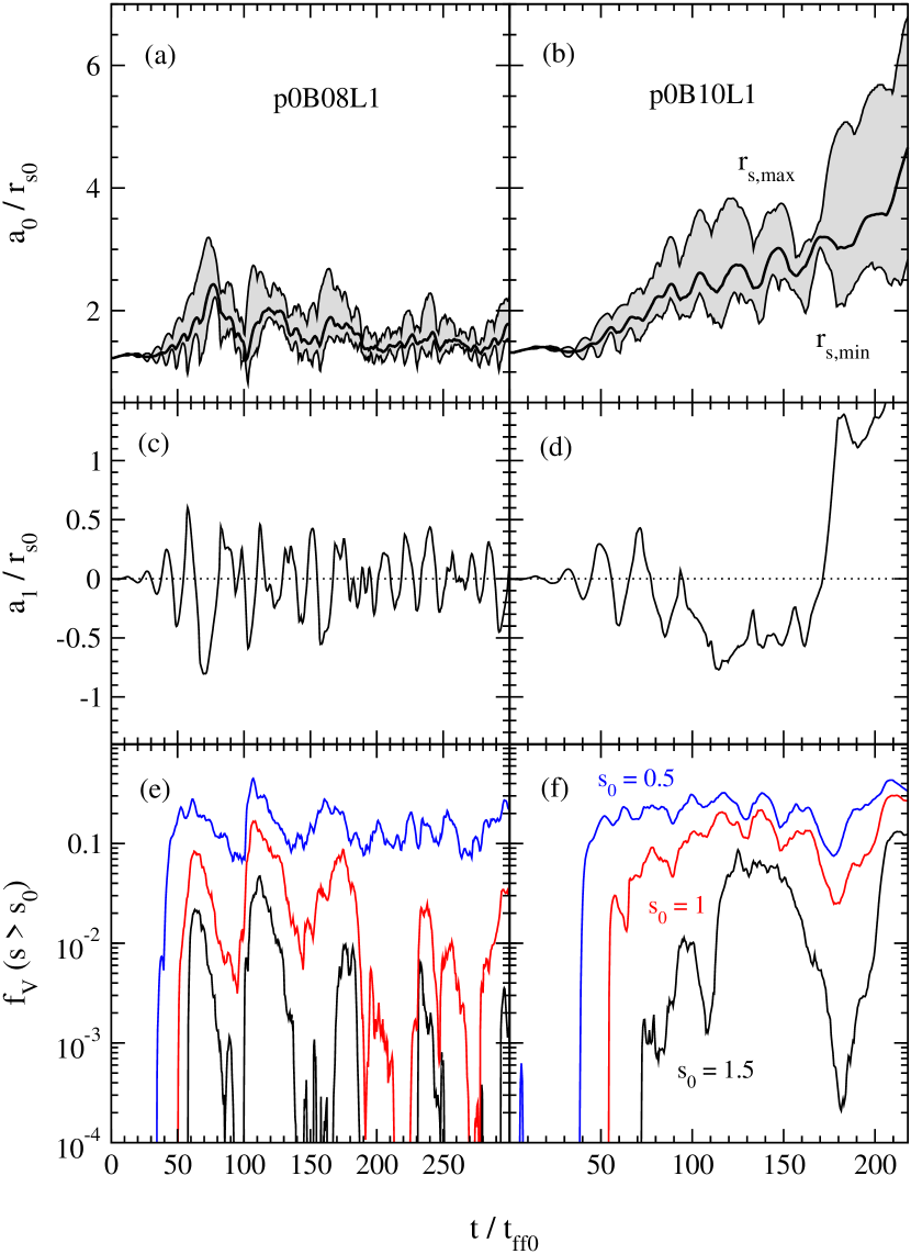
The characteristic behavior of models with an early dominance of the SASI is illustrated in Figures 2 and 3. Initially, the shock Legendre coefficient displays sinusoidal oscillations of exponentially growing amplitude. While in models without heating the SASI grows in amplitude until oscillations saturate while keeping its characteristic period (e.g., Fernández & Thompson 2009b), in models with significant heating this period increases when the amplitude becomes large, and eventually the regularity of the oscillation is lost.
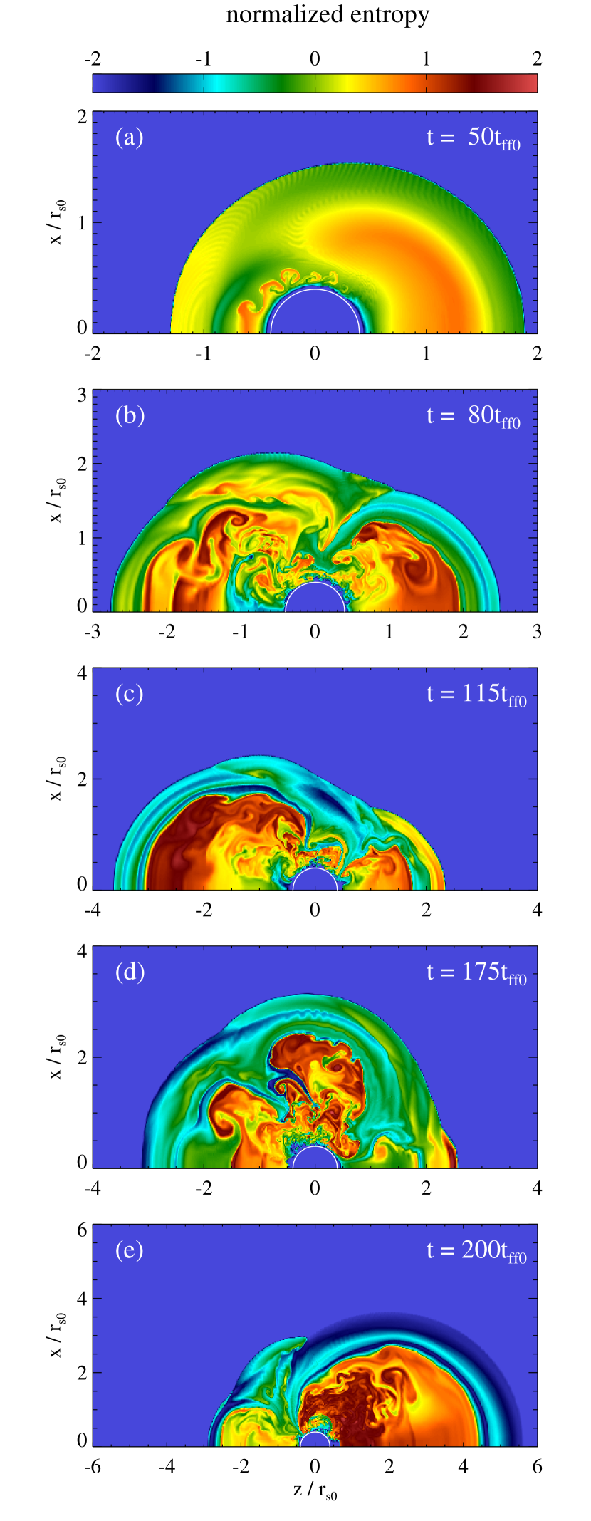
This breakdown of the SASI cycle is due to large-scale, long-lived fluid parcels with enhanced entropy emerging in the post-shock region. These structures are seeded during shock expansions (Figure 3a; see also Scheck et al. 2008). For small shock displacements, these elongated bubbles are shredded by lateral flows inherent in the SASI, and are advected out of the gain region, allowing the advective-acoustic cycle to proceed as in the case without heating. Above a certain amplitude, however, bubbles are able to resist shredding, and the SASI cycle is interrupted. Accretion proceeds then along narrow downflows that circumvent the bubbles (Figure 3b).
To quantitatively analyze the interplay between sloshing of the post-shock region and large-scale bubbles, we compare in Figure 2 the evolution of the shock Legendre coefficient , where
| (18) |
with the fraction of the post-shock volume with entropy higher than a fiducial value :
| (19) |
where the entropy
| (20) |
is defined so that it vanishes below the shock in the initial model ( and are the initial post-shock pressure and density, respectively; e.g. Foglizzo et al. 2007), and the post-shock volume is defined as
| (21) |
We use volume instead of mass to minimize the influence of low-entropy downflows. The emergence of peaks in for high values of the entropy is related to the loss of periodicity and eventual halting of shock sloshings, while bubble destruction can allow regular periodicity to emerge again (c.f. Figure 2c,e in the range ).
Large-scale bubbles that have halted the SASI can nevertheless be broken when low-entropy downflows bend and flow laterally. This process triggers bubble disruption, and results in their shredding or displacement to the opposite hemisphere (Figure 3). Accretion is then able to proceed through the whole hemisphere previously occupied by the bubble, and the shock executes a sloshing (c.f. Figure 2d,f in the range , also Figure 3d). The shock retractions are related to a decrease in pressure support triggered by an increase in cooling. The buoyancy of high-entropy bubbles blocks the flow of gas to the cooling region, resulting in a lower amount of cooling per SASI cycle and a loss of periodicity in the shock oscillations.
The key difference between exploding and non-exploding models appears to be whether the system can form entropy perturbations of sufficient size and amplitude. Model p0B10L1 displays such an entropy enhancement at time . This enhancement is perturbed and displaced around time , triggering a large sloshing of the shock that transitions into runaway expansion. In contrast, model p0B08L1 fails to develop a long-lived structure with entropy higher than . The transition to explosion for a large enough bubble results from the relative importance of buoyancy and drag forces (Thompson, 2000).
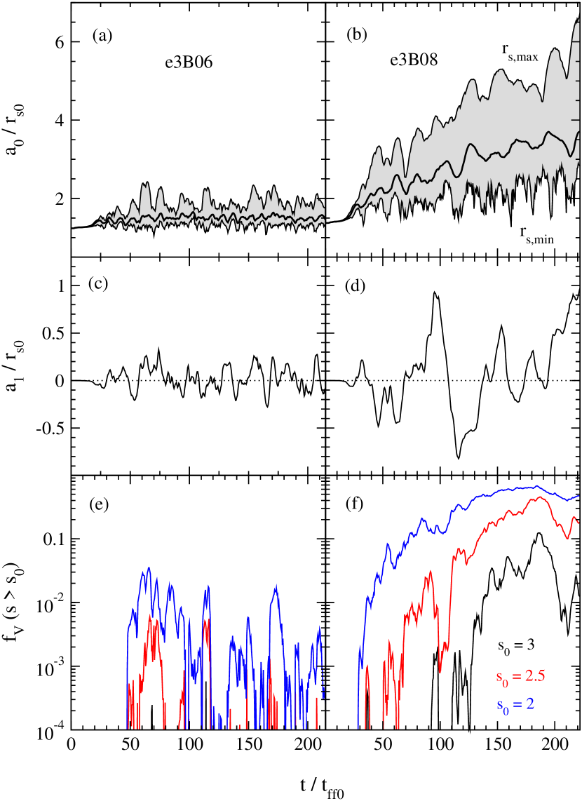
The characteristic evolution of convection-dominated models is illustrated by Figure 4. Entropy enhancements are initially generated by convection. Bubbles grow and merge into large-scale structures, which cause non-linear shock displacements. In non-exploding models, bubbles have a short lifetime, and hence the shock undergoes sloshings of moderate amplitude over a range of temporal frequencies. Note that the destruction of large bubbles can also lead to shock sloshings, but the persistent generation of entropy fluctuations of smaller scale and amplitude prevent the emergence of SASI oscillations with a well-defined periodicity.
For high enough heating rate, large bubbles are able to survive for many eddy turnover times, leading to explosion in a manner similar to that of SASI-dominated models. The role of high-entropy bubbles in convection-dominated models has been documented previously (Dolence et al., 2013; Couch, 2013a).
3.1.2 Effect of Initial Perturbations
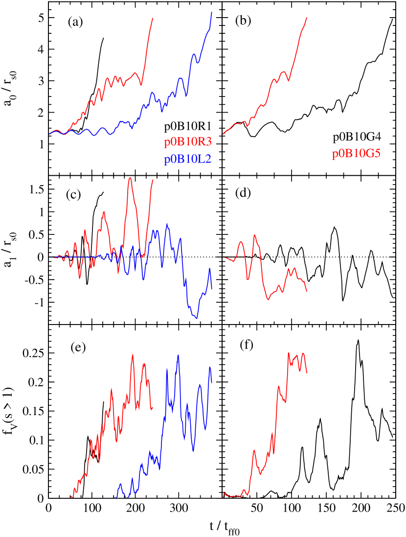
The effect of different initial perturbations on the exploding model of the e0 sequence is illustrated in Figure 5. Models with large amplitude random cell-to-cell density perturbations (p0B10R1 and pB10R3) follow the same path as the model where is directly perturbed (p0B10L1, Fig. 2). The model with an perturbation (p0B10L2) undergoes a weak convective phase over a number of advection times, during which grows and saturates at a small amplitude. After a delay of , however, oscillations of the shock emerge, and the model joins the usual SASI-dominated explosion path. The models with large amplitude density perturbations in the gain region with a fixed and dependence (p0B10G4 and p0B10G5) trigger less regular sloshings of the shock, which however still result in the formation of large-scale bubbles. As with the perturbation, an even- convective perturbation takes longer to couple to an SASI mode.
The time to explosion appears to be a non-trivial function of the perturbation form and amplitude. Model p0B10R3 has larger amplitude perturbations, yet it hits the outer boundary dynamical times later than model p0B10R1. Despite the very large amplitude perturbation of model p0B10G4, it explodes later than all models with an odd perturbation. This strong sensitivity to initial conditions has been documented previously by Scheck et al. (2006).
We emphasize however that we are focusing on models that are barely above the threshold for explosion. Recently, Couch & Ott (2013) have pointed out the importance of pre-collapse perturbations in tilting the balance towards explosion. Such an effect is likewise only going to make a difference if a model is already close to exploding in the absence of perturbations. For instance, models e0B10 and p0B10L1 differ in the type and amplitude of perturbations, leading to explosions that differ by more than dynamical times in onset. In contrast, neither of models e0B08 or p0B08L1 explode, despite the fact that they mirror the exact perturbations as the previous two exploding models (the latter having a density perturbation in the form of a thin shell).
From our results it is not obvious that a large enough density perturbation suffices to turn a model for which the background state is SASI-dominated into a convectively dominated model. Note however that our models have . Previous studies have witnessed more sensitivity to the type of initial perturbation when the parameter at shock stalling is close to or even transiently exceeds criticality (Scheck et al., 2008; Hanke et al., 2013).
The ‘purity’ of an excited SASI mode also depends on whether the background flow allows for unstable harmonics. Figure 1 shows that the first overtone is unstable for all the heating rates in the e0 sequence. This may lead to shock oscillations that are not a clean sinusoid, but which should not be mistaken as an imprint of convection.
3.2 Properties of the Quasi-Steady State
We now address the properties of the turbulent flow in the gain region in cases where an explosion is not obtained, focusing on the differences between models where either SASI or convection dominate. We first discuss general properties of the time-averaged flow, and then analyze models using a spherical Fourier-Bessel decomposition in space and a discrete Fourier transform in time.
3.2.1 Time-Averaged Flow and Convective Stability
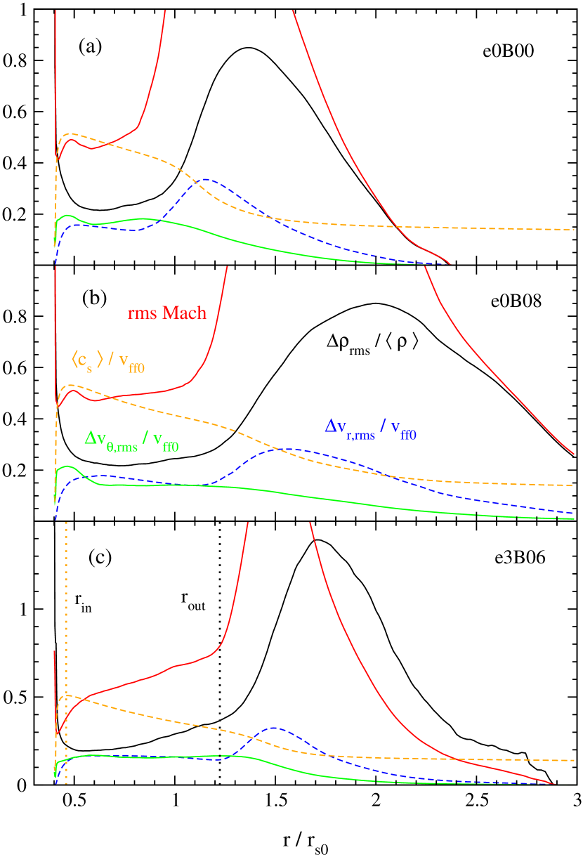
The spatial structure of the quasi-steady-state becomes clear when the flow is averaged in angle and time (e.g., Fernández & Thompson 2009b). Figure 6 shows such a representation for a model without heating (e0B00), as well as SASI- and convection-dominated models close to an explosion (e0B08 and e3B06, respectively). The time- and angle-average of a generic scalar quantity is denoted by
| (22) |
where is the time interval considered for the average, and the corresponding root-mean-square (r.m.s.) fluctuation is defined as
| (23) |
All three models share a basic general structure. From the inside out, this structure is composed of a narrow cooling layer adjacent to , a region of sub-sonic turbulence encompassing part of the cooling layer and part of the (time-averaged) gain region, an extended zone of shock oscillation, and the unperturbed upstream flow.
The most notorious difference among these models lies in the properties of the shock oscillation zone and in the flow around the cooling layer. Models where the SASI dominates have a wider shock oscillation zone than the model where convection is dominant. This can be seen by comparing the minimum and maximum shock radii of the non-exploding models in Figures 2 and 4. Also, in models where the SASI is prominent there is a bump in the r.m.s lateral velocity in the cooling layer, indicating strong shear. This bump is absent in the convection-dominated model.
In contrast, the subsonically turbulent region has very similar properties in the three different models shown in Figure 6, with only slight changes in the radial slopes. Characteristic values are , r.m.s. Mach number , and . This similarity in time-averaged properties suggests that flows are not very different from each other.
By analogy with convective systems in steady-state (e.g., nuclear burning stars), one can investigate whether the time-averaged system adjusts itself to a state of marginal convective stability. In hydrostatic systems, convection acts to erase destabilizing gradients, whereas the presence of advection in core-collapse supernova flows generates a non-zero entropy gradient in steady-state (Murphy & Meakin, 2011). One can nevertheless ask whether the relevant critical parameter for convection is restored to stability in the non-linear regime.
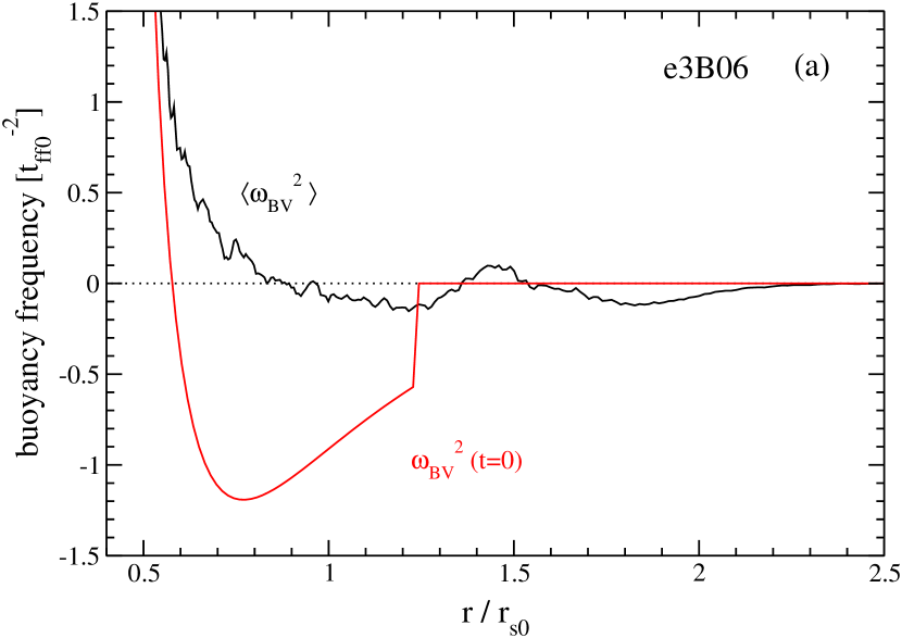
Figure 7a shows the initial and time-averaged squared buoyancy frequency (eq. [7]) for model e3B06, which is convection dominated. This model has an initial value of (Table 1). The time-averaged flow is such that the degree of convective instability (negative ) is significantly weaker than that in the initial state. The implications for convective stability become clear when the parameter (eq. [6]) is computed for the time-average flow. One way of doing this is simply averaging in time and angle, . However, because this is a non-linear function of the flow variables, the resulting value will not only capture the properties of the mean flow, but it will also include the contribution of turbulent correlations in the pressure, density, and velocity. One can nevertheless still define a convection parameter based on the properties of the mean flow
| (24) |
where the integral extends over regions where .
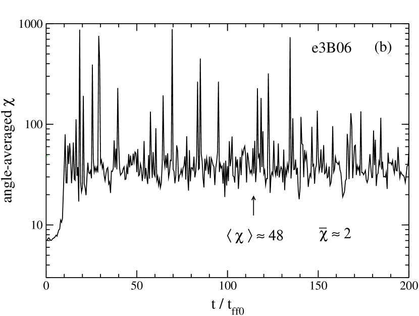
The difference between these two ways of computing is illustrated in Figure 7b. Shown is the instantaneous angle-averaged value of , together with its time average as well as the convection parameter computed using the mean flow, (eq. [24]). The instantaneous angle-averaged value of achieves very large values as soon as the shock displacement becomes non-linear, similar to the results of Burrows et al. (2012), with a time-averaged value . The convection parameter from the mean flow is much smaller, however, yielding . This small number arises from the small magnitude of the time-average of the squared buoyancy frequency shown in Figure 7a.
Values of for all non-exploding models are shown in Table 1. All convection-dominated models satisfy , which indicates that in quasi-steady-state they adjust to a state of convective sub-criticality (the equivalent of ‘flat’ entropy gradients in hydrostatic systems). The SASI-dominated models maintain , where is the value of in the initial condition. This increase in the time-averaged value of the convection parameter can arise from the increase in the size of the gain region caused by SASI activity, and from the presence of localized entropy gradients induced by the SASI, which trigger secondary convection (e.g., Figure 3a).
It is worth emphasizing that the driving agent matters in characterizing convective motions: secondary convection is qualitatively different from neurino-driven convection in that in the former there are both preferred spatial and temporal scales (entropy perturbations induced by the SASI, and advection time, respectively).
Another aspect of the explosion mechanism that can be probed with the time-averaged flow is the dependence of the turbulent kinetic energy in the gain region on neutrino heating. Hanke et al. (2012) found that a good indicator of the proximity of an explosion is the growth of the turbulent kinetic energy on the largest spatial scales. Since the mass in the gain region also increases due to the larger average shock radius, it is worth clarifying the origin of the increase in the kinetic energy. Table 1 shows the ratio of the total time-averaged turbulent kinetic energy in the gain region to the time-averaged mass in the gain region for non-exploding models. SASI-dominated models are such that this ratio is nearly constant, decreasing slightly when an explosion is closer. Thus larger kinetic energy is due solely to the increase in the mass of the gain region. In contrast, convection-dominated models grow both the specific kinetic energy and the mass in the gain region as an explosion is closer.
3.2.2 Properties of Turbulence in the Subsonic Region
We now use the spherical Fourier-Bessel expansion to analyze the properties of the turbulence in the subsonic region of the time-averaged flow. Operationally, we define the radial limits of this region ( and , §2.2) to be the peak of the time-averaged sound speed, , and the time-average of the minimum shock radius minus its r.m.s. fluctuation, , respectively. This definition differs from that of Murphy & Meakin (2011) in that we restrict ourselves to radii below the minimum shock position to avoid supersonic flow.
To connect with previous studies, we use the meridional velocity as a proxy for the turbulent flow. We do not multiply this velocity by , however, because the density stratification over the extended radial range considered would affect the spectral slopes (Endeve et al., 2012). Thus, the sum of the total power (eq. [17]) does not approach the total kinetic energy in the subsonic region, but instead it is a measure of the kinetic energy per unit mass.
Figure 8 shows 2D projections of the 3D space-time spectrum (eq. [17]), for pure SASI, SASI-dominated, and convection-dominated models (c.f. Figure 6). Power is maximal at low angular and radial scales, as expected from the inverse turbulent cascade in 2D (e.g., Davidson 2004). Models where the SASI is prominent display two characteristic features: (1) an even-odd pattern in the radial spectrum for , indicating the presence of discrete modes, and (2) enhanced power around the frequency corresponding to the advection time of the mean flow, . The dominance of convection manifests as a broadening of the smoother component of the spatial spectrum to larger and , a near disappearance of the even-odd pattern, and the emergence of power at temporal frequencies below and above . This behavior of SASI- and convection-dominated models in the frequency-domain is consistent with the results of Müller et al. (2012) and Burrows et al. (2012).
Figure 9 shows the results of contracting the array along two dimensions, yielding one dimensional spectra, for models that do not explode. In SASI-dominated models, the normalized power as a function of shows a characteristic sawtooth shape, which is smoothed to clarify the slope (an example of an non-smoothed spectrum is shown by the gray curve in Figure 9a).
Increasing the heating rate leads to minor changes in the (normalized) radial spectrum in SASI-dominated models. The onset of convection, on the other hand, leads to a shift of power from to . The spectral slope at large is approximately . This slope could be attributed to Rayleigh-Taylor turbulence, for which the velocity fluctuations satisfy , with the wavelength of the perturbation (e.g., Niemeyer & Woosley 1997; Ciaraldi-Schoolmann et al. 2009). Note however that the wave numbers of the radial basis functions of different are not harmonic with each other (Fig. 14), hence one cannot straightforwardly map radial wavelength into index . Nevertheless, the spacing between wave numbers becomes nearly constant at large , with only a linear shift with , motivating the use of as a differential measure of the turbulent cascade.
The angular spectrum in SASI-dominated models shows a peak at , and a slope at large indicative of a direct vorticity cascade (Kraichnan, 1967). Similar to the radial spectrum, the onset of convection results in the shift of power from towards . The resulting spectral shape has a form similar to that found by Hanke et al. (2012), Couch (2013a), and Dolence et al. (2013), who radially averaged the kinetic energy over a thin slice. This shape consists of a shallow curved shape at low , transitioning to slope at large .
The temporal spectrum of the sequence of convection-dominated models is consistent with the results of Burrows et al. (2012). At very low heating rates, a prominent peak exists at the advection frequency , indicating the presence of the SASI. As the heating rate is increased, power increases at frequencies below and above the advection peak. At heating rates close to an explosion, this low-frequency power is comparable or higher than that at .
In contrast, the SASI-dominated sequence has a dominant peak at the advection frequency for all models. This peak moves to lower frequencies as heating is increased, because the advection time increases given the larger average shock radius (Table 1). Also, the peak becomes broader as a likely result of secondary convection being triggered by the SASI. Power at the lowest frequencies still increases with heating rate, but it remains below that in the advection peak by at least a factor of two (in contrast, neutrino-driven convection yields a nearly flat spectrum). Note also that the power at frequencies higher than the advection peak in model e0B08 (SASI-dominated model with the highest heating) is within a factor of two of the convection-dominated model with the highest heating (e3B06).
From Figure 6 one can infer the turnover time of large eddies to be , yielding a frequency . Thus, the increase in power at frequencies below the advection time appears to be associated with the evolution of large bubbles in the gain region.
3.3 Application to Full-Scale Core-Collapse Models
Here we analyze the models of Müller et al. (2012) with the same methods used in our parametric models, identifying similarities and differences.
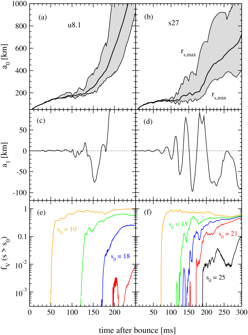
Figure 10 shows the evolution of the and coefficients for models u8.1 and s27, together with the fraction of the volume with entropy higher than fiducial values per baryon. The diagnostic behaves similarly to exploding parametric models p0B10L1 and e3B08 (Figs. 2 and 4). After a large enough fraction of the postshock volume is occupied by high entropy material, the regular periodicity of shock oscillations in model s27 is modified ( ms). Shock sloshings in this late stage are preceded by partial disruption of bubbles. One notable difference with model p0B10L1 is the emergence of secondary shocks in model s27, which prevent complete disruption of high-entropy bubbles. Runaway expansion in model s27 is preceded by accretion of the Si/O composition interface. Another important difference between both Müller et al. (2012) models and the exploding parametric models is the level of oscillations, which is much larger in the exploding gamma-law simulations222The difference in shock expansion rate once runaway starts is due to the absence of alpha particle recombination in the parametric models (Fernández & Thompson, 2009a); this is independent of the level of oscillations..
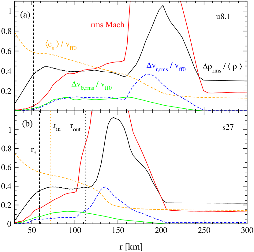
Models u8.1 and s27 both undergo a quasi-stationary phase that precedes runaway expansion. We have analyzed the properties of the time-averaged flow over the interval ms and ms in models u8.1 and s27, respectively. During these intervals, both the average shock radius and the average neutrinospheric radius (defined as the isodensity surface g cm-3) change by less than . Figure 11 shows the resulting profiles of time-averaged quantities, in analogy with Figure 6. Above the neutrinosphere, all quantities behave in the same qualitative way as the parametric models. At densities g cm-3 and higher, clear differences are introduced by the existence of a protoneutron star, however. In particular, the density and velocity fluctuations decrease significantly inside , whereas Figure 6 shows a strong increase in the density perturbation near for parametric models due to the accumulation of mass given the reflecting boundary condition, and a bump in the lateral velocity due to shear in SASI-dominated cases. Nonetheless, the very similar behavior of the system outside shows that a reflecting boundary condition is not a bad approximation.
We have also computed the convection parameter using the time-averaged flow (eq. [24]). The buoyancy frequency is computed following Müller et al. (2013) but ignoring relativistic corrections333The leading order corrections to the buoyancy frequency and sound speed scale like (Müller et al., 2013), which is only a few percent in the gain region.. Model u8.1 has , consistent with the hypothesis that convection-dominated flow adjusts itself to sub-criticality. This parameter is even smaller () in model s27.
Figure 12 shows one-dimensional spectra of the subsonic region in models u8.1 and s27. The limits of the region are defined to be the saddle point in the time- and angle-averaged sound speed on the inside, and the time-average of the minimum shock radius minus its rms fluctuation on the outside (both radii are shown in Figure 11 for s27). The radial spectrum of the Müller et al. (2012) models has relatively less power at long wavelengths than the parametric models. At short wavelengths, however, the spectral slope is similar, and the sawtooth pattern of SASI-dominated models is also present in model s27 (the spectrum extends to due to the compactness of the subsonic region relative to the grid spacing). The angular spectrum of model s27 shows the same peak at as the SASI-dominated parametric models. Model u8.1 shows a similar curved shape as convection-dominated models, though with some excess at and . Finally, the temporal spectrum shows clearly the distinction between convection-dominance manifesting more power at low frequencies (u8.1), and SASI-dominance generating a clear peak at the advection time (s27). This temporal frequency behavior was already noted by Müller et al. (2012).
In summary, the general results from parametric models regarding SASI- and convection-dominated flow persist in sophisticated, full-scale core-collapse simulations. The use of nuclear dissociation in parametric models as the control parameter for switching between SASI- and convection-dominance does not prevent qualitative agreement with full-scale models, even though the latter always have dissociation present. This is because the behavior of the flow depends chiefly on the relative timescales of the system (c.f. §2.1.3).
4 Summary and Discussion
We have analyzed the transition to explosion in SASI- and convection-dominated
core-collapse supernova explosions using parametric, two-dimensional,
time-dependent hydrodynamic simulations. These models are such that
the linear stability properties are well understood, allowing the
exploration of well-differentiated regions of parameter
space (Figure 1, Table 1).
We have also introduced a spherical Fourier-Bessel decomposition
to characterize the properties of turbulence in the sub-sonic
region of the flow, to extract signatures of the interplay
of SASI and convection. Our main findings are as follows:
1. – The behavior of SASI-dominated models is characterized by the
interplay of shock sloshings and the formation of large-scale,
high-entropy structures. These bubbles are seeded by the SASI
during shock expansions. Regular sloshing of the shock requires that
these bubbles have a short lifetime and/or small entropy enhancements.
Regular destruction of high-entropy structures by lateral flows
is characteristic of non-exploding models (Figure 2).
2. – Models that explode with SASI dominance are able to form large-scale,
high-entropy bubbles that survive for a time longer than a
characteristic shock oscillation cycle (Figure 2). Neutrino heating and
the inverse turbulent cascade in 2D ensure that these bubbles
continue to grow if left undisturbed. Explosion results from the buoyancy
of the bubble overcoming the drag force of the upstream flow (Thompson, 2000).
3. – Convection-dominated models generate similar large-scale
entropy structures by consolidating smaller-scale bubbles arising from
buoyant activity. Sloshing of the shock occurs whenever large bubbles are
destroyed or displaced, just as in SASI-dominated models, but without
a dominant periodicity. The transition to explosion also involves the
formation and growth of a sufficiently
large bubble (Figure 4), as has been documented
previously (Dolence et al., 2013; Couch, 2013a).
4. – Initial perturbations with a large amplitude do not alter the
qualitative way in which SASI-dominated models explode in two dimensions.
The difference in explosion time can be significant, however, and the
time to runaway is not a monotonic function of the
perturbation amplitude (Figure 5).
5. – The time-averaged flow in convection-dominated, non-exploding models adjusts itself to a state in which the convection parameter computed
from the mean flow (eq. [24]) lies below
the critical value for convective instability (Table 1).
This phenomenon is obscured when an average value of is computed
from the instantaneous flow (Figure 7).
6. – The spherical Fourier-Bessel power in the subsonic, weakly-stratified
region is dominated by
the largest spatial scales (Figure 8). The SASI
manifests itself as a characteristic
even-odd pattern in the radial direction, and enhanced power at temporal frequencies
corresponding to the advection time. Convection generates a smoother component,
with power concentrated primarily below the advection frequency. This
behavior of the frequency domain is consistent with the results of
Burrows
et al. (2012) and Müller
et al. (2012).
7. – The slope of the angular spectrum is consistent with
an inverse turbulent cascade at large . Convection-dominated
models yield angular spectra that resemble those of Hanke et al. (2012),
Couch (2013a), and Dolence et al. (2013),
while SASI-dominated models show a peak at .
The radial spectrum shows a scaling at large , which
could be associated with Rayleigh-Taylor turbulence (e.g., Ciaraldi-Schoolmann
et al. 2009).
8. – The general results obtained with the parametric models persist when
the analysis is repeated on the general relativistic, radiation-hydrodynamic simulations
of Müller
et al. (2012). In particular, the behavior of the entropy when
approaching explosion, and the value of the convection parameter and
spectral slopes of the time-averaged flow are in good agreement with the
corresponding parametric models.
9. – The equality between advection and heating times in the gain region at is a good
indicator of the onset of non-oscillatory instability in one-dimensional numerical
simulations of parametric models (Appendix A), in agreement with the
numerical results of Fernández (2012). The fact that this
equality occurs for heating rates such that the linear eigenmodes are still
oscillatory (Figure 1), however, means that the onset of
purely growing expansion is a non-linear
effect (growth time shorter than the oscillation period).
Initial equality between the advection time in the gain and cooling layers
is a good indicator of instability in some regions of the space of
parametric models, but not in others, particularly when nuclear dissociation is included
(Figure 1). When the recombination energy from alpha
particles is not accounted for, the onset of instability does not necessarily
lead to an explosion (Appendix A), thus the instability thresholds do not
equal explosion criteria for the parametric setup.
Our results show that despite the non-linearity of the flow, clear signatures of the operation of the SASI and convection can be obtained. In particular, the parameter (equation 6) – evaluated at the time where the shock stalls and before hydrodynamic instabilities set in – is a good predictor of whether the system will be SASI- or convection-dominated on its way to explosion.
Despite the different explosion paths obtained when SASI or convection dominate the dynamics at early times, it is not clear that the resulting explosion properties are very different once the process has started. Our results indicate that in both cases, the formation of at least one large-scale, high-entropy bubble is a necessary condition to achieve explosion in two-dimensions. It may be that this degeneracy is triggered by the inverse turbulent cascade inherent in axisymmetric models.
The absence of this inverse cascade in 3D causes the flow to develop more small-scale structure than in 2D (e.g., Hanke et al. 2012). Nonetheless, the tendency of bubbles to merge into bigger structures will persist, as this is an intrinsic property of the Rayleigh-Taylor instability (Sharp, 1984). In fact, several 3D hydrodynamic studies have observed that prior to explosion, a large-scale asymmetry (often ) develops in a non-oscillatory way (Iwakami et al., 2008; Couch, 2013a; Dolence et al., 2013; Hanke et al., 2013). The difference lies in the fact that the SASI provides seeds for large-scale entropy fluctuations independent of dimension, so it can speed up the formation of a large- and hot enough bubble to achieve explosion. Verifying whether this picture is robust requires numerical experiments in 3D.
Even though we have found clear evidence for high entropy bubbles playing a key role in the interplay between SASI and convection and in the onset of explosion, there are many questions that remain to be answered. First, the evolution of the diagnostic suggests that transition to explosion in a multidimensional environment involves a fraction of the gain region volume achieving a certain entropy or positive energy. What is that volume or mass fraction, and what are the required entropy or energy values as a function of the dominant system parameters?
Second, our characterization of large bubble dynamics in the gain region is limited. Processes such as seeding of bubbles by shock displacements, survivability of bubbles due to neutrino heating, buoyancy, and the turbulent cascade, disruption by lateral SASI flows in the linear phase or low-entropy plumes in the non-linear phase, and feedback of these bubbles on SASI modes deserve further study. Preliminary steps in this direction have already been taken (e.g., Guilet et al. 2010; Couch 2013a; Dolence et al. 2013; Murphy et al. 2013), though much more work remains if a quantitative understanding – in the form of a predictive explosion criterion – is to be attained.
It is interesting to compare the critical heating rates for explosion in our parametric models and those from lightbulb setups with a full EOS and a time-dependent mass accretion rate (e.g., Nordhaus et al. 2010; Hanke et al. 2012; Couch 2013a). In the former, explosion occurs above (but close to) the instability threshold in both SASI- and convection-dominated models, with only a difference between 1D and 2D (Fig. 1). In contrast, the latter models are such that non-spherical instabilities make a larger difference () relative to the 1D case, with explosion occurring for heating rates below the oscillatory instability. Note however that both classes of models neglect the (negative) feedback to the heating rate due to the drop in accretion luminosity when the shock expands, thus the numbers obtained from these models should be treated with caution. The search for a robust and predictive explosion criterion valid for both SASI- and convection-dominated models is a worthwhile pursuit, though outside the scope of the present paper.
The modification of our results by the introduction of a third spatial dimension will be addressed in future work.
Acknowledgements
We thank Jeremiah Murphy, Sean Couch, Christian Ott, Jérôme Guilet, Adam Burrows, Josh Dolence, Yudai Suwa, Kei Kotake, Ernazar Abdikamalov, and Annop Wongwathanarat for stimulating discussions. The authors thank the Institute for Nuclear Theory at the University of Washington for its hospitality, and the US Department of Energy for partial support during the completion of this work. The anonymous referee provided helpful comments that improved the presentation of the paper. RF is supported by NSF grants AST-0807444, AST-1206097, and the University of California Office of the President. BM and HJ are supported by the Deutsche Forschungsgemeinschaft through the Transregional Collaborative Research Center SBF-TR7 “Gravitational Wave Astronomy” and the Cluster of Excellence EXC 153 “Origin and Structure of the Universe”. TF is supported by the grant ANR-10-BLAN-0503 funding the SN2NS project. The software used in this work was in part developed by the DOE NNSA-ASC OASCR Flash Center at the University of Chicago. Parametric models were evolved at the IAS Aurora cluster, while the Garching models were evolved on the IBM p690 of the Computer Center Garching (RZG), on the Curie supercomputer of the Grand Équipement National de Calcul Intensif (GENCI) under PRACE grant RA0796, on the Cray XE6 and the NEC SX-8 at the HLRS in Stuttgart (within project SuperN), and on the JUROPA systems at the John von Neumann Institute for Computing (NIC) in Jülich.
Appendix A On the Stability of the SASI mode
Here we compare the predictions from timescale ratio diagnostics with the actual eigenfrequencies of the mode in the parametric system.
Figure 13 shows the shock radius as a function of time for one dimensional (1D) versions of the e0 and e3 sequences shown in Table 1. By comparing with Figure 1, one can see that the oscillatory radial stability thresholds are well captured at this resolution. The initial value of the ratio of advection time in the gain region to advection time in the cooling region is a good indicator of oscillatory radial stability for the sequence, but not so much when nuclear dissociation is introduced.
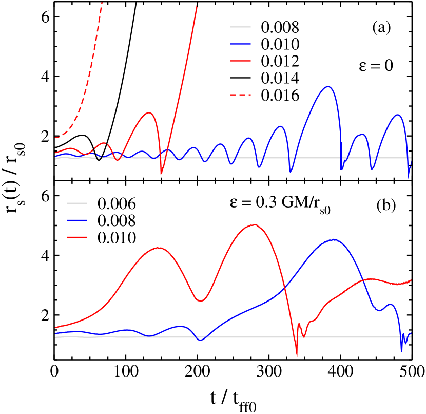
The initial ratio of advection to heating times in the gain region is a good predictor of non-oscillatory expansion in the 1D models, in agreement with the numerical results of Fernández (2012). Note however that for both sequences, this point lies at a lower heating rate than the bifurcation of the perturbative growth rate (Fig. 1). Therefore, this runaway expansion is a non-linear effect, likely arising from the fact that the growth time is shorter than the oscillation period (by more than a factor of two in the e0 model when the ratio of advection to heating timescales is unity).
Note also that in contrast to the models of Fernández (2012), radial instability does not always lead to runaway expansion. This is clear from the model with and , which saturates. Also, all the models with nuclear dissociation saturate. Fernández & Thompson (2009a) showed that this effect is due to the artificial assumption of constant nuclear dissociation at the shock. Including the recombination energy of alpha particles as the shock expands (which decreases the effective dissociation rate), leads to a runaway as soon as instability sets in.
Appendix B Spherical Fourier-Bessel Decomposition in between Concentric Shells
In spherical polar coordinates, the general solution to the Helmholtz equation444Since the Laplacian operator is Hermitian, its eigenfunctions – solutions to the Helmholtz equation – form a complete orthogonal basis in the Hilbert space (Arfken & Weber, 2005). is a superposition of functions of the form (e.g., Jackson 1999)
| (25) |
where and are the spherical Bessel functions, are the Laplace spherical harmonics, and are constant coefficients. The wavenumber and the coefficients are determined once boundary conditions for the problem are imposed at the radial domain boundaries and .
B.1 Dirichlet Boundary Conditions
Requiring that the eigenfunctions vanish at the radial boundaries for all yields the system of equations
| (26) |
Non-trivial solutions are obtained by setting the determinant of the matrix of coefficients to zero. This condition then defines a discrete set of radial wavenumbers:
| (27) | |||
where labels the roots in increasing magnitude.
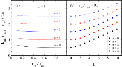
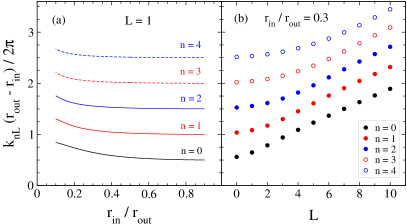
Figure 14a shows the first five solutions for , as a function of the ratio of boundary radii . We adopt the convention of labeling the smallest wavenumber by , since the eigenfunction has no nodes. For low , the relation
| (28) |
holds approximately, becoming better for . Increasing the angular degree increases the value of the wave number relative to equation (28), as shown in Figure 14b.
Equation (26) also determines the ratio of coefficients
| (29) |
Note that has been added as an index to the coefficients. The radial eigenfunctions are then
| (31) | |||||
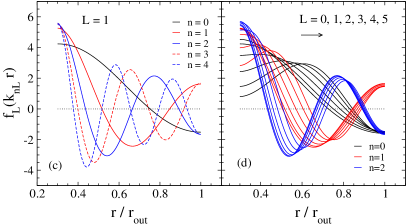
where the two formulations differ only by a global (real) phase. The normalization constant is found from the orthogonality condition (Lommel integral). Combining two solutions of the spherical Bessel differential equation, integrating over the radial domain, applying the boundary conditions, and using L’Hôpital’s rule yields
| (32) | |||||
where is the Kronecker symbol and primes denote derivative respect to the argument. For the first formulation (eq. 31), choosing
| (33) | |||||
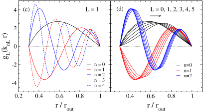
makes the eigenfunctions orthonormal. Figure 15 shows two examples of the resulting normalized eigenfunctions in a two dimensional, axisymmetric space.
In three dimensions, the expansion of an arbitrary function with Dirichlet boundary conditions in the radial interval can be written as
| (34) |
with coefficients given by
| (35) |
where the star denotes complex conjugation. The corresponding Parseval identity is
| (36) |
yielding a three-dimensional spatial power spectrum:
| (37) |
B.2 Neumann Boundary Conditions
Requiring that the radial derivative of the eigenfunctions vanish at the boundaries yields the equation for the radial wave numbers
| (38) | |||
where the primes again denote derivative respect to the argument. The eigenfunctions are now
| (39) | |||||
| (40) | |||||
and the orthogonality condition reads
| (41) |
The normalization constant for equation (39) is
| (42) | |||||
The radial wave numbers and eigenfunctions for the first few harmonics and values are shown in Figure 16. The overall structure of the wave numbers is very similar to the Dirichlet case, with slightly higher values for small ratio of radii and large . For fixed harmonic, the eigenfunctions change their shape as is increased, in contrast to the Dirichlet case.
References
- Arfken & Weber (2005) Arfken G. B., Weber H. J., 2005, Mathematical Methods for Physicists, sixth edn. Elsevier, Amsterdam
- Arnett & Meakin (2011) Arnett W. D., Meakin C., 2011, ApJ, 733, 78
- Bethe (1990) Bethe H. A., 1990, Reviews of Modern Physics, 62, 801
- Bethe & Wilson (1985) Bethe H. A., Wilson J. R., 1985, ApJ, 295, 14
- Blondin & Mezzacappa (2006) Blondin J. M., Mezzacappa A., 2006, ApJ, 642, 401
- Blondin & Mezzacappa (2007) Blondin J. M., Mezzacappa A., 2007, Nature, 445, 58
- Blondin et al. (2003) Blondin J. M., Mezzacappa A., DeMarino C., 2003, ApJ, 584, 971
- Blondin & Shaw (2007) Blondin J. M., Shaw S., 2007, ApJ, 656, 366
- Bruenn et al. (2006) Bruenn S. W., Dirk C. J., Mezzacappa A., Hayes J. C., Blondin J. M., Hix W. R., Messer O. E. B., 2006, Journal of Physics Conference Series, 46, 393
- Buras et al. (2006) Buras R., Janka H.-T., Rampp M., Kifonidis K., 2006, A&A, 457, 281
- Buras et al. (2006) Buras R., Rampp M., Janka H.-T., Kifonidis K., 2006, A&A, 447, 1049
- Burrows (2013) Burrows A., 2013, RMP, 85, 245
- Burrows et al. (2012) Burrows A., Dolence J. C., Murphy J. W., 2012, ApJ, 759, 5
- Burrows et al. (1995) Burrows A., Hayes J., Fryxell B. A., 1995, ApJ, 450, 830
- Burrows et al. (2007) Burrows A., Livne E., Dessart L., Ott C. D., Murphy J., 2007, ApJ, 655, 416
- Ciaraldi-Schoolmann et al. (2009) Ciaraldi-Schoolmann F., Schmidt W., Niemeyer J. C., Röpke F. K., Hillebrandt W., 2009, ApJ, 696, 1491
- Couch (2013a) Couch S. M., 2013a, ApJ, 775, 35
- Couch (2013b) Couch S. M., 2013b, ApJ, 765, 29
- Couch & Ott (2013) Couch S. M., Ott C. D., 2013, ApJL, submitted, arXiv:1309.2632
- Davidson (2004) Davidson P. A., 2004, Turbulence: an introduction for scientists and engineers, first edn. Oxford University Press, Oxford
- Dolence et al. (2013) Dolence J. C., Burrows A., Murphy J. W., Nordhaus J., 2013, ApJ, 765, 110
- Dubey et al. (2009) Dubey A., Antypas K., Ganapathy M. K., Reid L. B., Riley K., Sheeler D., Siegel A., Weide K., 2009, J. Par. Comp., 35, 512
- Endeve et al. (2012) Endeve E., Cardall C. Y., Budiardja R. D., Beck S. W., Bejnood A., Toedte R. J., Mezzacappa A., Blondin J. M., 2012, ApJ, 751, 26
- Fernández (2010) Fernández R., 2010, ApJ, 725, 1563
- Fernández (2012) Fernández R., 2012, ApJ, 749, 142
- Fernández & Thompson (2009a) Fernández R., Thompson C., 2009a, ApJ, 703, 1464
- Fernández & Thompson (2009b) Fernández R., Thompson C., 2009b, ApJ, 697, 1827
- Fisher et al. (1995) Fisher K. B., Lahav O., Hoffman Y., Lynden-Bell D., Zaroubi S., 1995, MNRAS, 272, 885
- Foglizzo (2009) Foglizzo T., 2009, ApJ, 694, 820
- Foglizzo et al. (2007) Foglizzo T., Galletti P., Scheck L., Janka H.-T., 2007, ApJ, 654, 1006
- Foglizzo et al. (2006) Foglizzo T., Scheck L., Janka H.-T., 2006, ApJ, 652, 1436
- Fryer & Young (2007) Fryer C. L., Young P. A., 2007, ApJ, 659, 1438
- Guilet & Foglizzo (2012) Guilet J., Foglizzo T., 2012, MNRAS, 421, 546
- Guilet et al. (2010) Guilet J., Sato J., Foglizzo T., 2010, ApJ, 713, 1350
- Hammer et al. (2010) Hammer N. J., Janka H.-T., Müller E., 2010, ApJ, 714, 1371
- Hanke et al. (2012) Hanke F., Marek A., Müller B., Janka H.-T., 2012, ApJ, 755, 138
- Hanke et al. (2013) Hanke F., Müller B., Wongwathanarat A., Marek A., Janka H.-T., 2013, ApJ, 770, 66
- Herant et al. (1994) Herant M., Benz W., Hix W. R., Fryer C. L., Colgate S. A., 1994, ApJ, 435, 339
- Iwakami et al. (2008) Iwakami W., Kotake K., Ohnishi N., Yamada S., Sawada K., 2008, ApJ, 678, 1207
- Jackson (1999) Jackson J. D., 1999, Classical Electrodynamics, third edn. Wiley, Hoboken
- Janka (2001) Janka H.-T., 2001, A&A, 368, 527
- Janka (2012) Janka H.-T., 2012, Ann. Rev. Nuc. Part. Sci., 62, 407
- Janka et al. (2012) Janka H.-T., Hanke F., Hüdepohl L., Marek A., Müller B., Obergaulinger M., 2012, Prog. Th. Ex. Phys., 2012, 010000
- Janka & Keil (1998) Janka H.-T., Keil W., 1998, in L. Labhardt, B. Binggeli, & R. Buser ed., Supernovae and cosmology Perspectives of Core-Collapse Supernovae beyond SN 1987A. p. 7
- Janka & Müller (1996) Janka H.-T., Müller E., 1996, A&A, 306, 167
- Kifonidis et al. (2006) Kifonidis K., Plewa T., Scheck L., Janka H.-T., Müller E., 2006, A&A, 453, 661
- Kraichnan (1967) Kraichnan R. H., 1967, Physics of Fluids, 10, 1417
- Marek & Janka (2009) Marek A., Janka H.-T., 2009, ApJ, 694, 664
- Mezzacappa et al. (1998) Mezzacappa A., Calder A. C., Bruenn S. W., Blondin J. M., Guidry M. W., Strayer M. R., Umar A. S., 1998, ApJ, 495, 911
- Müller et al. (2010) Müller B., Janka H.-T., Dimmelmeier H., 2010, ApJS, 189, 104
- Müller et al. (2012) Müller B., Janka H.-T., Heger A., 2012, ApJ, 761, 72
- Müller et al. (2013) Müller B., Janka H.-T., Marek A., 2013, ApJ, 766, 43
- Müller et al. (2012) Müller E., Janka H.-T., Wongwathanarat A., 2012, A&A, 537, 63
- Murphy & Burrows (2008) Murphy J. W., Burrows A., 2008, ApJ, 688, 1159
- Murphy et al. (2013) Murphy J. W., Dolence J. C., Burrows A., 2013, ApJ, 771, 52
- Murphy & Meakin (2011) Murphy J. W., Meakin C., 2011, ApJ, 742, 74
- Niemeyer & Woosley (1997) Niemeyer J. C., Woosley S. E., 1997, ApJ, 475, 740
- Nordhaus et al. (2010) Nordhaus J., Brandt T. D., Burrows A., Livne E., Ott C. D., 2010, PRD, 82, 103016
- Nordhaus et al. (2010) Nordhaus J., Burrows A., Almgren A., Bell J., 2010, ApJ, 720, 694
- Ohnishi et al. (2006) Ohnishi N., Kotake K., Yamada S., 2006, ApJ, 641, 1018
- Ott et al. (2008) Ott C. D., Burrows A., Dessart L., Livne E., 2008, ApJ, 685, 1069
- Ott et al. (2013) Ott C. D., et al., 2013, ApJ, 768, 115
- Press et al. (2006) Press W. H., Teukolski S. A., Vetterling W. T., Flannery B. P., 2006, Numerical Recipes in Fortran 77, second edn. Cambridge University Press, Cambridge
- Rampp & Janka (2002) Rampp M., Janka H.-T., 2002, A&A, 396, 361
- Scheck et al. (2008) Scheck L., Janka H.-T., Foglizzo T., Kifonidis K., 2008, A&A, 477, 931
- Scheck et al. (2006) Scheck L., Kifonidis K., Janka H.-T., Müller E., 2006, A&A, 457, 963
- Sharp (1984) Sharp D. H., 1984, Physica D Nonlinear Phenomena, 12, 3
- Suwa et al. (2010) Suwa Y., Kotake K., Takiwaki T., Whitehouse S. C., Liebendörfer M., Sato K., 2010, PASJ, 62, L49
- Takiwaki et al. (2012) Takiwaki T., Kotake K., Suwa Y., 2012, ApJ, 749, 98
- Thompson (2000) Thompson C., 2000, ApJ, 534, 915
- Thompson et al. (2005) Thompson T. A., Quataert E., Burrows A., 2005, ApJ, 620, 861
- Wongwathanarat et al. (2010) Wongwathanarat A., Janka H.-T., Müller E., 2010, ApJ, 725, L106
- Wongwathanarat et al. (2013) Wongwathanarat A., Janka H.-T., Müller E., 2013, A&A, 552, 126
- Woosley et al. (2002) Woosley S. E., Heger A., Weaver T. A., 2002, Reviews of Modern Physics, 74, 1015
- Yamasaki & Yamada (2007) Yamasaki T., Yamada S., 2007, ApJ, 656, 1019