A fast map-making preconditioner for regular scanning patterns
Abstract
High-resolution Maximum Likelihood map-making of the Cosmic Microwave Background is usually performed using Conjugate Gradients with a preconditioner that ignores noise correlations. We here present a new preconditioner that approximates the map noise covariance as circulant, and show that this results in a speedup of up to 400% for a realistic scanning pattern from the Atacama Cosmology Telescope. The improvement is especially large for polarized maps.
I Introduction
As the resolution and sensitivity of Cosmic Microwave Background (CMB) experiments increase, so do the computational resources needed to analyze their data. Because modern detectors are background-limited, the only way to significantly increase sensitivity is to increase the number of detectors. The last decades have seen an increase from tens of detectors to thousands of detectors in experiments like ACT Dünner et al. (2013); Niemack et al. (2010), SPT Carlstrom et al. (2011); Austermann et al. (2012), POLARBEAR Kermish et al. (2012) and Keck Kernasovskiy et al. (2012), and plans already exist for experiments with detectors Abazajian et al. (2013). Reducing the data from all these detectors into a coherent map of the sky presents a significant computational challenge, and already with 1000-detector-class experiments this step is the most important bottleneck of the data analysis pipeline Dünner et al. (2013). It is therefore important to investigate ways to speed up this process.
Three main classes of map-makers are in popular use: Maximum likelihood map-makers Tegmark (1997); Cantalupo et al. (2010); de Gasperis et al. (2005); Traficante et al. (2011); Dünner et al. (2013); QUIET Collaboration et al. (2012), which are slow, but produce unbiased, optimally noise-weighted maps; faster but slightly less accurate destripers Keihänen et al. (2005); Sutton et al. (2010); and biased and sub-optimal but very fast naive map-makers QUIET Collaboration et al. (2012); Schaffer et al. (2011). The topic of this paper is a method for significantly speeding up maximum likelihood map-makers.
Assuming a linear detector response, we can model the time-ordered data via the the linear system
| (1) |
where is the pixelized map of the sky, the pointing matrix is a sparse111The pointing matrix will be sparse if we solve for a beam-convolved map. For variable beams or asymmetric beams, one may want to reconvolve to a standard beam as part of map-making. This can be done using , at the cost of some of its sparsity. We do not consider this case here. matrix mapping from pixels to samples, and is the time-domain noise, which we assume to be gaussian with covariance matrix . The maximum likelihood solution for is given by the map-making equation Tegmark (1997),
| (2) |
This is of the form , and while the matrices involved are usually too large to solve by direct inversion, the system is amenable to solution by Preconditioned Conjugate Gradients (PCG) Press et al. (2007) provided a good preconditioner can be found222Without a preconditioner, the number of iterations needed for conjugate gradients is proportional to the condition number of the matrix . By applying a preconditioner , one is effectively solving the system . The goal is then to choose such that is as well-conditioned as possible. This can be acchevied if .. The most commonly used map-making preconditioners are the binned Natoli et al. (2001); Ashdown et al. (2007); Cantalupo et al. (2010) and Jacobi Doré et al. (2001); de Gasperis et al. (2005); Cantalupo et al. (2010); Dünner et al. (2013) preconditioners. The binned preconditioner approximates the time covariance matrix as diagonal (i.e. it ignores correlations), which for pointing matrices where only one pixel is hit per sample results in a diagonal pixel-space covariance matrix.
| (3) | ||||
| (4) |
The Jacobi preconditioner simplifies one step further, and assumes that every detector has the same variance, , resulting in
| (5) |
The proportionality factor is usually set to 1, as PCG is insensitive to an overall scaling of the preconditioner.


The assumption of independent noise is quite inaccurate. All realistic experiments have at least some time-correlation in the noise, and usually also correlations between different detectors. Additionally, filters will also generally introduce correlations.
While computing the full, exact is often too expensive, single rows of it can be computed at the same expense as one CG iteration:
| (6) |
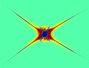
Here is the pixel-space basis vector corresponding to pixel . An example of what such a row looks like for the Atacama Cosmology Telescope (ACT) Dünner et al. (2013) can be seen in figure 1.
It is clear that the approximation of no correlation is quite inaccurate. However, since the correlation structure is driven by the scanning pattern and relative position of the detectors in the focalplane, the correlation structure should be the same for all pixels which are scanned the same way. ACT, which used long-duration, small-amplitude drift scans, pixels at the same declination but different right ascension will be hit by the same phase of the same scanning motion, and should therefore have the same correlation structure.333 Circulant correlation is not a good approximation for every experiment. It is suitable for constant elevation dift scans, as employed by ACT, SPT and POLARBear, but we expect it to work poorly for full-sky scanning patterns.
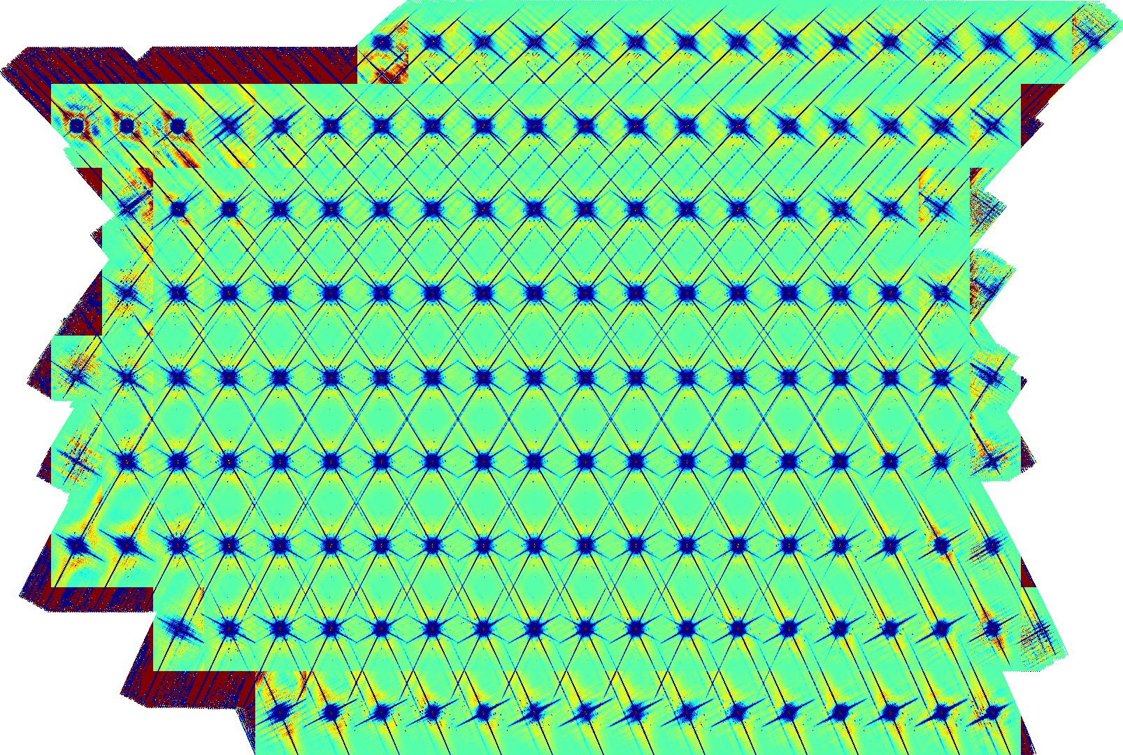
Indeed, that is what measurements show (see figure 2). It may therefore be a good approximation to assume that every point in the map has the same relative correlation structure, i.e. that the correlation between two points on the sky only depends on their relative position. If this is the case, then it is possible to choose a pixelization where the correlation only depends on the difference between pixel numbers, and hence that the pixel correlation matrix is circulant444 For example, if , where are coordinates, then a pixelization scheme , where is a pixel index and G is a linear function will fulfill , resulting in a circulant correlation matrix..
A circulant matrix has the nice property of being diagonal in the frequency domain, which means that it can be computed, stored and applied cheaply, at the cost of a few FFTs. Hence, the constant correlation approximation is promising as a preconditioner for solving the map-making equation.
II Implementation
The inverse pixel covariance matrix can be decomposed into variance and correlation such that . Here is diagonal (block-diagonal in the case of polarization) in pixel space, and corresponds to a map of the inverse standard deviation per pixel. As per the binned preconditioner, this can be approximated as
| (7) |
The correlation matrix is in general a dense matrix, but as noted above, it can often be approximated as circulant555The matrix will be circulant provided that the correlation structure is position-independent, that a constant offset in each coordinate corresponds to a constant pixel offset, and provided that indices wrap around at the edges.. Therefore, the constant correlation preconditioner replaces with a circulant matrix , such that
| (8) |
This relation can be inverted to give us an expression for in terms of ,
| (9) | ||||
| (10) |
Since is circulant, i.e. , we have
| (11) |
using forward and backwards Fourier transforms and , where is the number of rows in the matrix.
With this in hand, the preconditioner can be applied as
| (12) |
and can be precomputed, so the cost of applying the preconditioner is simply that of two FFTs and three diagonal matrix multiplications.
The choice of the reference pixel at which the correlation is measured is somewhat arbitrary. We used the pixel nearest the center of the map, but other locations not too close to the edge of the map should also work.
III Regularization
While constant correlation is a good approximation for relatively short-scale correlations, it works less well for long-distance correlations, and regions near the edges666Near the edges the telescope must decelerate in order to reverse the scanning direction, which makes the correlation structure different there than in the center. Applying the preconditioner as described above to realistic cases results in the appearance of large scale modes which change extremely slowly during the subsequent CG iteration.
A way around this is to artificially limit the range of the correlations that are modeled, by multiplying by a Gaussian. For ACT, a standard deviation of 20 pixels was found to be effective, but this will depend on the scanning pattern, and some experimentation may be needed to find the optimal number.
IV Polarization
The previous discussion assumed that each pixel only had a single degree of freedom, e.g. temperature-only maps of the sky. In the case of polarization, each pixel has several correlated components, typically the Stokes parameters T, Q and U Zaldarriaga & Seljak (1997), but this can instead be expressed as a larger number of block-correlated single-component pixels. This results in being block-diagonal with e.g. one (T,Q,U)-block per physical pixel, while becomes a vector of similar blocks. And instead of a single row of needing to be measured, all the rows corresponding to a given physical pixel now need to be computed (i.e. for all components, where Greek indices indicate polarization components). Hence, eq. (10) becomes
| (13) |
Aside from that, everything works the same.
V Test setup
| Step 5 | Step 15 | Step 45 | Step 115 | Step 340 | |
|---|---|---|---|---|---|
|
Binned |
 |
 |
 |
 |
 |
|
Const. corr. |
 |
 |
 |
 |
 |
| Step 15 | Step 70 | Step 250 |
|---|---|---|
 |
 |
 |
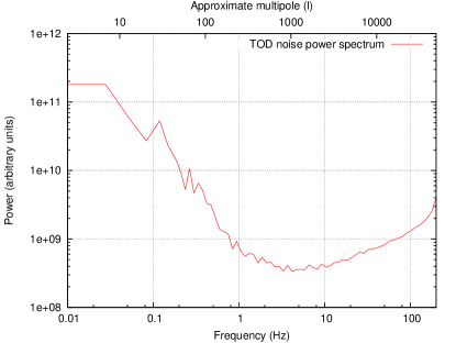
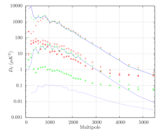
We tested the preconditioners on a simulated time-ordered data (TOD) based on the scanning pattern for 64 detectors from each of 417 15-minute scans of a subset of ACT’s southern patch centered at . Each scan was a constant elevation drift scan with amplitude of in azimuth, and the scan centers were spread over 10 steps in elevation, covering a patch of about by degrees. Odd steps in elevation scanned while rising and the even ones when setting. This resulted in most pixels being hit from two directions, and hence the x-shaped correlation pattern seen in figures 1-2. An example of a noise power spectrum used in the simulation can be seen in figure 3.
The simulated detectors were polarization-sensitive, with each detector measuring a linear combination of the local radiation field, with each detector having a different, randomly chosen detector angle . While an ACT-like noise model, including the effects of atmosphere and inter-detector noise correlations was assumed in the map-making step, no noise was added to the simulated TOD in order to allow the convergence to be studied all the way to the highest multipoles777 This is valid since the convergence rate of PCG is mostly independent of the noise level of the right-hand side after the first few iterationsNatoli et al. (2001). However, with higher noise, higher CG errors also become acceptable, so the number of iterations needed for CG errors to be subdominant will be smaller for realistic noise levels.. For the same reason, the simulated input CMB did not include a beam, and was pixelated at the same resolution as the output map, in order to avoid subpixel noise.
We then solved the map-making equation for this data set using PCG, first using the binned preconditioner described in equation (4), and then the constant correlation approximation described in this paper. Each was run for 600 CG iterations, with intermediate maps being output for every 5 steps.
VI Results
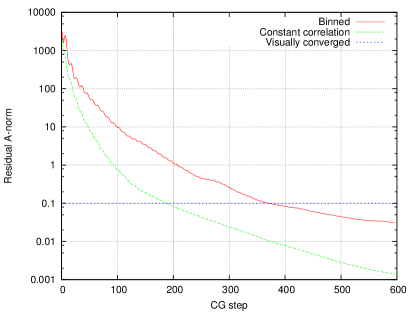
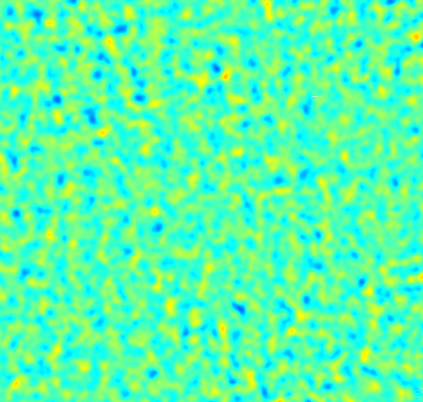
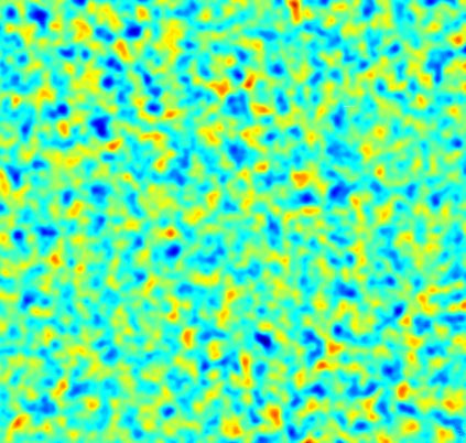
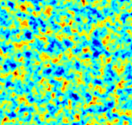
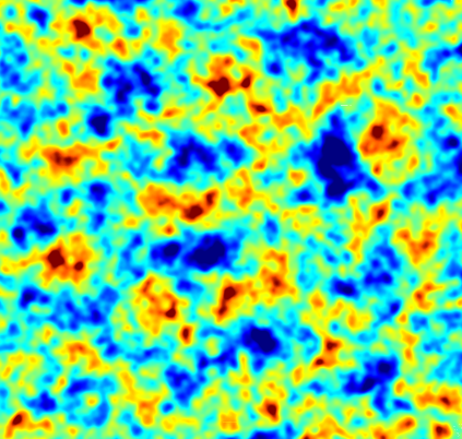
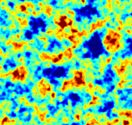
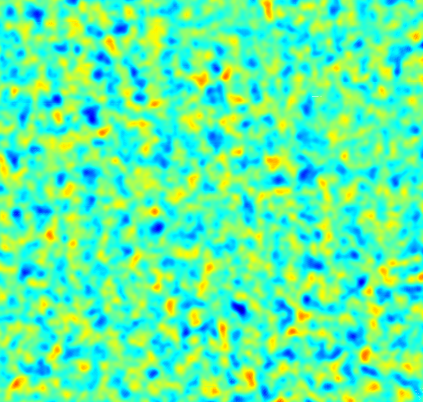
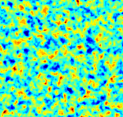
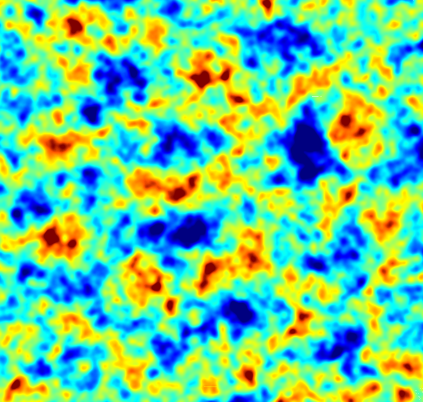
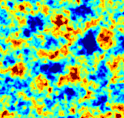
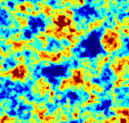
The constant correlation preconditioner visually converges roughly 3 times faster than the binned one, as shown for the temperature map in figure 5. Likewise, the residual A-norm Strakos & Tichy (2008) from the CG solver (shown in figure 4) also shows a significant improvement in convergence: roughly a factor 2 according to this metric888The A-norm of a vector is defined as , where is in our case. The error A-norm after CG steps is , where is our estimate after steps, and is the true map. When the true is unknown, can be estimated as , where and are two internal variables in the CG algorithm at step , and is is an integer that controls the accuracy of the estimate (4 in our case).
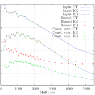
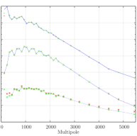
However, neither of these tests take into account the fact that not all scales in the map are equally interesting. To remedy this, figure 6 compares the binned and constant correlation power spectra with that of the simulated input map. These spectra were computed using the method described in Louis et al. (2013). On large scales (), this tells the same story as the maps did: The larger the scale, the more slowly it converges, with the constant correlation preconditioner being about 3 times faster than the binned one. Somewhat surprisingly, a similar phenomenon occurs at the small scales. For , higher results in slower convergence, and this is especially prominent for the EE and BB power spectra. On all scales, however, the constant correlation preconditioner appears to converge several times faster than the binned one.
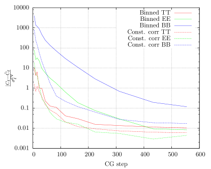
In order to quantify the convergence more precisely, we consider the time at which the absolute error in a given multipole-bin reaches 0.1 times cosmic variance in that bin. While somewhat arbitrary, this choice ensures that CG errors are guaranteed to be sub-dominant in the power spectrum, regardless of the noise properties of the actual experiment. Figure 7 shows the convergence of TT, EE and BB for both preconditioners for a typical multipole-bin. The overall trend for each component is an initial rapid fall followed by a slower decay, with both being significantly faster for the new preconditioner, particularly for the polarization spectra.
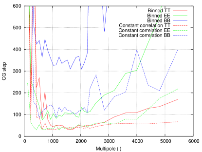
We found that binning the errors in bins of conjugate gradients steps and using linear interpolation between these bins resulted in a robust estimate of when each spectrum bin reaches the convergence criterion. The resulting convergence times can be seen in figure 8, and confirm our earlier finding that the largest and smallest scales converge more slowly. The figure also highlights how much trouble the binned preconditioner has with the EE and especially BB spectra, where it performs much more poorly relative the constant correlation preconditioner than we see for the TT spectrum. We speculate that this is due to the X-shaped correlation structure introduced by our scanning pattern. In binned maps, which ignore the correlations, this introduces spurious X-shaped patterns in both Q and U, corresponding to spurious signal in both E and B. With the constant correlation preconditioner, these are partially corrected because some of the correlation structure is taken into account.
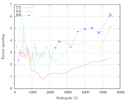
We summarize the performance characteristics of the new preconditioner in figure 9, which shows its relative speed gain vs. the baseline binned preconditioner. Depending on , we have a speedup ranging from 20% to 200% for TT, from 150% to 300% for EE, and from 200% to 400% for BB, with the greatest relative improvement happening at the scales that converge most slowly.
VII Summary
The structure of a CMB map’s pixel covariance matrix is determined by the noise properties of the time-ordered data and the scanning pattern of the telescope. For constant elevation drift scans like those employed by ACT, SPT and POLARBEAR, this results in an approximately circulant covariance. We have developed a new preconditioner for conjugate gradient solutions of the map-making equation which exploit this property by deconvolving the correlations in harmonic space, an operation which is very cheap due to the Fourier representation of a circulant matrices being diagonal.
For a realistic scanning pattern and noise model the preconditioner results a speedup of 20% to 200% for temperature and 150% to 400% for polarization compared to a binned preconditioner.
Convergence speed might potentially be further improved by allowing the correlation pattern to change slowly across the map, for example by decomposing the map into overlapping tiles, and applying the constant correlation preconditioner separately to each tile, followed by a merging operation. Our preliminary attempts at such a tiled preconditioner have however not been able to beat the simple constant correlation approximation presented here.
Acknowledgements.
The authors would like to thank Jo Dunkley and Johannes Noller for useful discussion and suggestions, and Jon Sievers for testing the preconditioner in another map-maker. We also thank the ACT collaboration for access to internal ACT data used in the simulations. Computations were performed on the gpc supercomputer at the SciNet HPC Consortium. SciNet is funded by: the Canada Foundation for Innovation under the auspices of Compute Canada; the Government of Ontario; Ontario Research Fund - Research Excellence; and the University of Toronto. SN and TL are supported by ERC grant 259505.References
- Abazajian et al. (2013) Abazajian, K. N., Arnold, K., Austermann, J., et al. 2013, ArXiv e-prints, arXiv:1309.5383
- Ashdown et al. (2007) Ashdown, M. A. J., Baccigalupi, C., Balbi, A., et al. 2007, A&A, 467, 761
- Austermann et al. (2012) Austermann, J. E., Aird, K. A., Beall, J. A., et al. 2012, in Society of Photo-Optical Instrumentation Engineers (SPIE) Conference Series, Vol. 8452, Society of Photo-Optical Instrumentation Engineers (SPIE) Conference Series
- Cantalupo et al. (2010) Cantalupo, C. M., Borrill, J. D., Jaffe, A. H., Kisner, T. S., & Stompor, R. 2010, ApJS, 187, 212
- Carlstrom et al. (2011) Carlstrom, J. E., Ade, P. A. R., Aird, K. A., et al. 2011, PASP, 123, 568
- de Gasperis et al. (2005) de Gasperis, G., Balbi, A., Cabella, P., Natoli, P., & Vittorio, N. 2005, A&A, 436, 1159
- Doré et al. (2001) Doré, O., Teyssier, R., Bouchet, F. R., Vibert, D., & Prunet, S. 2001, A&A, 374, 358
- Dünner et al. (2013) Dünner, R., Hasselfield, M., Marriage, T. A., et al. 2013, ApJ, 762, 10
- Keihänen et al. (2005) Keihänen, E., Kurki-Suonio, H., & Poutanen, T. 2005, MNRAS, 360, 390
- Kermish et al. (2012) Kermish, Z. D., Ade, P., Anthony, A., et al. 2012, in Society of Photo-Optical Instrumentation Engineers (SPIE) Conference Series, Vol. 8452, Society of Photo-Optical Instrumentation Engineers (SPIE) Conference Series
- Kernasovskiy et al. (2012) Kernasovskiy, S., Ade, P. A. R., Aikin, R. W., et al. 2012, in Society of Photo-Optical Instrumentation Engineers (SPIE) Conference Series, Vol. 8452, Society of Photo-Optical Instrumentation Engineers (SPIE) Conference Series
- Louis et al. (2013) Louis, T., Næss, S., Das, S., Dunkley, J., & Sherwin, B. 2013, ArXiv e-prints, arXiv:1306.6692
- Natoli et al. (2001) Natoli, P., de Gasperis, G., Gheller, C., & Vittorio, N. 2001, A&A, 372, 346
- Niemack et al. (2010) Niemack, M. D., Ade, P. A. R., Aguirre, J., et al. 2010, in Society of Photo-Optical Instrumentation Engineers (SPIE) Conference Series, Vol. 7741, Society of Photo-Optical Instrumentation Engineers (SPIE) Conference Series
- Press et al. (2007) Press, W. H., Teukolsky, S. A., Vetterling, W. T., & Flannery, B. P. 2007, Numerical Recipes 3rd Edition: The Art of Scientific Computing, 3rd edn. (Cambridge University Press)
- QUIET Collaboration et al. (2012) QUIET Collaboration, Araujo, D., Bischoff, C., et al. 2012, ApJ, 760, 145
- Schaffer et al. (2011) Schaffer, K. K., Crawford, T. M., Aird, K. A., et al. 2011, Astrophys. J. , 743, 90
- Strakos & Tichy (2008) Strakos, Z., & Tichy, P. 2008, ETNA, 13, 56
- Sutton et al. (2010) Sutton, D., Zuntz, J. A., Ferreira, P. G., et al. 2010, MNRAS, 407, 1387
- Tegmark (1997) Tegmark, M. 1997, ApJL, 480, L87
- Traficante et al. (2011) Traficante, A., Calzoletti, L., Veneziani, M., et al. 2011, MNRAS, 416, 2932
- Zaldarriaga & Seljak (1997) Zaldarriaga, M., & Seljak, U. 1997, Phys. Rev. D, 55, 1830