Nonlinear Compressive Particle Filtering

Abstract

Many systems for which compressive sensing is used today are dynamical. The common approach is to neglect the dynamics and see the problem as a sequence of independent problems. This approach has two disadvantages. Firstly, the temporal dependency in the state could be used to improve the accuracy of the state estimates. Secondly, having an estimate for the state and its support could be used to reduce the computational load of the subsequent step.

In the linear Gaussian setting, compressive sensing was recently combined with the Kalman filter to mitigate above disadvantages. In the nonlinear dynamical case, compressive sensing can not be used and, if the state dimension is high, the particle filter would perform poorly. In this paper we combine one of the most novel developments in compressive sensing, nonlinear compressive sensing, with the particle filter. We show that the marriage of the two is essential and that neither the particle filter or nonlinear compressive sensing alone gives a satisfying solution.

I Introduction

Compressive sensing (CS) [6, 13] has gained considerable attention the last decade. Its remarkable property of exactly estimating a linear system from far fewer measurements than what previously thought possible has inspired to many new interesting developments and applications.

The holy grail of compressive sensing is the ability to solve optimization problems of the form

$$\min_{\boldsymbol{x}}\|{\boldsymbol{x}}\|_{0}\quad{\mbox{subj. to}}\quad{\boldsymbol{y}}={\boldsymbol{A}}{\boldsymbol{x}}.$$ (1)

${\boldsymbol{x}}\in{\mathbb{R}}^{n}$ is here the sought parameter vector, ${\boldsymbol{A}}\in{\mathbb{R}}^{N\times n}$ a sensing matrix which is generally assumed known, and ${\boldsymbol{y}}\in{\mathbb{R}}^{N}$ a given vector of stacked measurements. For a detailed review of the literature, the reader is referred to several recent publications, such as [4] and [14].

One of the newest developments in compressive sensing is nonlinear compressive sensing (NLCS) [2, 3, 20]. In NLCS the measurement equation is not required to be linear. This is particularly interesting in applications where physical limitations make the measurement equation nonlinear. In e.g., X-ray crystallography and many applications in optics, only intensities are observed. Since ${\boldsymbol{x}}$ in these applications often is a complex valued vector, the phase information is lost when measuring. The measurement equation then takes the form

$${\boldsymbol{y}}=|{\boldsymbol{A}}{\boldsymbol{x}}|^{2},\quad{\boldsymbol{y}}\in{\mathbb{R}}^{N},\;{\boldsymbol{A}}\in\mathbb{C}^{N\times n},\;{\boldsymbol{x}}\in\mathbb{C}^{n},$$ (2)

where the absolute value and the square are acting elementwise on the complex vector ${\boldsymbol{A}}{\boldsymbol{x}}$. Other applications with this type of nonlinear measurement equation show up in e.g., diffraction imaging [5], astronomy [10, 15], optics [27], x-ray tomography [12], microscopy [18, 1, 24], and quantum mechanics [9] and the problem is often referred to as the phase retrieval problem.

Many systems that are of interest in compressive sensing are dynamical systems. The temporal relation between ${\boldsymbol{x}}$s are often neglected and compressive sensing applied repeatedly as if temporally consecutive ${\boldsymbol{x}}$s would be independent. It is rather obvious that taking into account the temporal relation between two consecutive ${\boldsymbol{x}}$s might improve estimation accuracy over treating two consecutive ${\boldsymbol{x}}$s as independent vectors. It might also be that an estimate of ${\boldsymbol{x}}$ at time $t$ can be used to reduce the computational load at time $t+1$.

In this paper we propose to combine nonlinear compressive sensing with particle filtering to estimate a sequence of sparse temporally dependent states. We will assume that the state support is unknown and estimate the state ${\boldsymbol{x}}$ and its support from measurements ${\boldsymbol{y}}$. We will show that this approach outperforms the alternative of neglecting the temporal relation between consecutive ${\boldsymbol{x}}$s. We also show that the problem can not be solved by a particle filter alone and hence that the marriage of the two is essential.

II Background

Nonlinear state estimation is a system theoretic problem of great scientific importance in many fields and application domains. In general the estimation problems are an extension of static nonlinear parameter estimation problems where the unknown parameter vector obeys a given dynamic propagation law. Such propagation laws can be given in either continuous or discrete time by a nonlinear differential or difference equation. A state estimation problem is characterized via three classes of information: (a) the dynamic propagation law, (b) the measurement equation characterizing the relationship between the measured quantity and the unknown state vector and (c) the noise quantities characterizing (one of) the driving forces of the dynamic propagation law and the measurement errors made. In this paper we do not consider deterministic (known) driving forces for the dynamic propagation laws.

Despite the major interest, a generic solution to the nonlinear state reconstruction problems for nonlinear models for (a) and (b) and arbitrary noise statistics is computational untractable. Therefore succesful solutions consists in specializing one or more of the information classes in the definition of nonlinear state estimation problems to “restrictive” circumstances and/or reciding to “approximate solutions”. One such famous family of algorithms are the so-called Extended Kalman filters where smooth nonlinear functions in the description (a) and (b) are assumed while the noise statistics are approximated by Gaussian probability density functions (see for instance [23]). Various improvements on these restrictions and/or assumptions were made since then. Here we mention the unscented Kalman filter (UKF) [17] and the derivative free nonlinear Kalman filter [21], set-membership state estimation [22], Ellipsoid state estimation [8] and the particle filter [16, 26].

An important specialization of the state reconstruction problem is for the case the unknown state vector is sparse. Thereby calling for a dynamic extension to the succesfull research line of reconstruction of a large unknown parameter vector in linear least squares problems from a limited number of measurements by imposing sparsity constraints, as in compressed sensing [6, 13]. Such a dynamic extension for linear dynamics and linear measurement equation has recently been studied in [25, 28, 7, 11]. In these recent approaches, we recognize two families of approaches to perform “sparse state reconstruction”. The first, like [7] integrates the $\ell_{1}$ norm constraints as a pseudo measurement in a classical minimum variance or $2$ norm (extended) Kalman filtering framework. Even for the case the dynamic propagation and measurement equation are linear, the $2$-norm approximation requires iterations inheriting all advantages and disadvantages of the extended Kalman filtering. The second class of filtering methods try in addition to the reconstruction of the state, to estimate its support as well. The sparsity estimation was dealt with in in [28] with a multiple of particle filters, whereby the large dimensional output vectors was mapped onto a lower dimensional space using classical ideas of compressive sensing. In [25] a combination of a classical generalized likelihood ratio testing for expanding (or decreasing) the unknown support set of the state vector is combined with classical reduced Kalman filtering. Later on the same author and collaborators in [11] have adapted the PF with an importance sampling step for predicting the possibly “abrupt” changes in the support of the state. That support prediction is based on classical $\ell_{1}$ regularization compressed sensing solutions for static linear measurement equations. In this paper a generalization to particle filters for nonlinear measurement equations is presented.

III Setup

We will assume that the state ${\boldsymbol{x}}$ follows a nonlinear process model with additive process noise and that the support (i.e., the set of indices corresponding to nonzero elements) of ${\boldsymbol{x}}$ is slowly varying. The state ${\boldsymbol{x}}$ will have dimension $n$ and the measurements ${\boldsymbol{y}}$ dimension $N$. We will restrict ourself to quadratic measurement equations. We do this to ease the notation and also because we believe that it is an important special case that provides a sufficiently good approximation of the nonlinearity in many applications of interest. As shown in [19], the extension to handle more general nonlinearities is rather trivial. We will for simplicity assume that the measurement noise ${\boldsymbol{w}}$ is additive and Gaussian. The process noise ${\boldsymbol{v}}$ will be assumed additive and with a probability density function (pdf) given by $p_{{\boldsymbol{v}}}(\cdot)$. $g:{\mathbb{R}}^{n}\rightarrow{\mathbb{R}}^{n}$ is the process function and $h:{\mathbb{R}}^{n}\rightarrow{\mathbb{R}}^{N}$ the measurement function with the $i$th element

$$\big{(}h({\boldsymbol{x}})\big{)}(i)=a_{i}+{\boldsymbol{b}}_{i}^{\mathsf{T}}{\boldsymbol{x}}+{\boldsymbol{x}}^{\mathsf{T}}{\boldsymbol{Q}}_{i}{\boldsymbol{x}},\,a_{i}\in{\mathbb{R}},{\boldsymbol{b}}_{i}\in{\mathbb{R}}^{n},{\boldsymbol{Q}}_{i}\in{\mathbb{R}}^{n\times n}.$$

$diag(\cdot)$ produces a quadratic matrix with its argument on the diagonal. In particular, if we let ${\boldsymbol{s}}(t)$ be a binary row vector of length $n$, the dynamical nonlinear model takes the form:

$${\boldsymbol{x}}(t+1)= diag({\boldsymbol{s}}(t))\left(g({\boldsymbol{x}}(t),t)+{\boldsymbol{v}}(t)\right),$$ (3a)

$${\boldsymbol{y}}(t)= h({\boldsymbol{x}}(t))+{\boldsymbol{w}}(t),$$ (3b)

$${\boldsymbol{w}}(t)\sim {\mathcal{N}}(0,{\boldsymbol{R}}),\,{\boldsymbol{v}}(t)\sim p_{{\boldsymbol{v}}},\,{\boldsymbol{x}}(t)\in{\mathbb{R}}^{n},\,{\boldsymbol{y}}(t)\in{\mathbb{R}}^{N}.$$ (3c)

For each of the elements in ${\boldsymbol{s}}(t)$, the binary value stays the same with probability $\alpha$ and the element is changed with probability $1-\alpha$ (basically a Markov chain). It is assumed that $\alpha$ is close to 1. The indices of the nonzero elements of ${\boldsymbol{s}}(t)$ make up the support. We will make the assumption that the number of elements in the support is rather small in comparison to the number of measurements $N$ and the state dimension $n$.

We will represent the distribution for the state ${\boldsymbol{x}}$ using particle approximations. If we denote the $i$th particle at time $t$ by ${\boldsymbol{x}}^{(i)}(t)$ and its corresponding weight by $w^{(i)}(t)$, the particle approximation using $M$ particles of the pdf of ${\boldsymbol{x}}(t)$ given ${\boldsymbol{s}}(t)$ and measurements up to time $t$ is

$$p({\boldsymbol{x}}(t)|\{{\boldsymbol{y}}(s )\}_{s=1}^{t},{\boldsymbol{s}}(t))$$

$$\approx \sum_{i=1}^{M}w^{(i)}(t)\delta\left({\boldsymbol{x}}(t)-diag({\boldsymbol{s}}(t)){\boldsymbol{x}}^{(i)}(t)\right).$$ (4)

$\delta(\cdot)$ is here used to denote the delta Dirac function. Similarly, we will let the particle approximation using $M$ particles of the pdf of the predicted state at time $t+1$, ${\boldsymbol{x}}(t+1|t)$, given ${\boldsymbol{s}}(t)$ and measurements up to time $t$, be given by

$$p({\boldsymbol{x}}(t+1|t)|\{{\boldsymbol{y}}(s)\}_{s=1}^{t},{\boldsymbol{s}}(t))$$

$$\approx\sum_{i=1}^{M}w^{(i)}(t+1|t)\delta\left({\boldsymbol{x}}(t+1|t)-diag({\boldsymbol{s}}(t)){\boldsymbol{x}}^{(i)}(t+1|t)\right).$$ (5)

Note that ${\boldsymbol{x}}(t+1|t)$ is used to denote the predicted state at time $t+1$ given measurements up to time $t$. We accordingly let $w^{(i)}(t+1|t)$ denote the predicted weight at time $t$ of particle $i$ and ${\boldsymbol{x}}^{(i)}(t+1|t)$ the predicted $i$th particle at time $t+1$, both using measurements up to time $t$.

IV Nonlinear Compressive Particle Filtering

In this paper we treat and analyze the problem of sparse estimation with nonlinear dynamics and quadratic measurement equations by combining ideas from particle filtering and nonlinear compressive sensing, and in particular quadratic basis pursuit (QBP) [20]. We believe that a second order Taylor expansion of the measurement function often is sufficient and therefore restrict the discussion to quadratic measurement functions.

We will describe the nonlinear compressive particle filter (NCPF) in detail in the following subsections, however, we start by giving a brief outline of the algorithm:

• Initialization: Given an estimate for ${\boldsymbol{s}}(0)$ and the number of particles to be used $M$. Generate $\{{\boldsymbol{z}}^{(i)}\}_{i=1}^{M}\in{\mathbb{R}}^{n}$ by sampling from some given initial distribution $p_{0}$. Initialize the particles $\{{\boldsymbol{x}}^{(i)}(1|0)\}_{i=1}^{M}\in{\mathbb{R}}^{n}$ by ${\boldsymbol{x}}^{(i)}(1|0)=diag({\boldsymbol{s}}(0)){\boldsymbol{z}}^{(i)},\,i=1,\dots,M$. Initialize the weights by $\{w^{(i)}(1|0)\}_{i=1}^{M}=1/M$. Form a particle approximation of the predictive distribution $p({\boldsymbol{x}}(1|0)|{\boldsymbol{s}}(0))$ by (5). Set the design parameter $\Delta t$, $\lambda$ and $\epsilon$. When ${\boldsymbol{y}}(1)$ becomes available, set $t=1$ and proceed to step 1.

• Propagate the Predictive Distribution One Step: Given ${\boldsymbol{y}}(t)$ and a particle approximation of the predictive distribution at time $t$, $p({\boldsymbol{x}}(t|t-1)|\{{\boldsymbol{y}}(s)\}_{s=1}^{t-1},{\boldsymbol{s}}(t-1))$, compute a particle approximation of the predictive distribution at time $t=t+1$, $p({\boldsymbol{x}}(t+1|t)|\{{\boldsymbol{y}}(s)\}_{s=1}^{t},{\boldsymbol{s}}(t-1))$, using ${\boldsymbol{s}}(t-1)$. Proceed to step 2.

• Add Elements to the Support: If the likelihood for the observations ${\boldsymbol{y}}(t)$, $p({\boldsymbol{y}}(t)|\hat{\boldsymbol{x}}(t))$, where $\hat{\boldsymbol{x}}$ is an approximation of the expected value of ${\boldsymbol{x}}(t)$, falls below some threshold, apply ideas from NLCS to detect what new elements of ${\boldsymbol{x}}$ are likely to be nonzero and add their indices to the support by updating ${\boldsymbol{s}}(t-1)$. Proceed to step 3.

• Remove Elements from the Support: If the mean of an element of ${\boldsymbol{x}}$ gets within some $\epsilon$-bound from zero and remains within this bound for $\Delta t$ consecutive time steps, exclude that element from the set of nonzero elements by setting corresponding element in ${\boldsymbol{s}}(t-1)$ to zero.

• Update the Predictive Distribution: If the support has changed, set ${\boldsymbol{s}}(t-\Delta t-1)={\boldsymbol{s}}(t-1)$, compute $p({\boldsymbol{x}}(t-\Delta t|t-\Delta t-1)|\{{\boldsymbol{y}}(s)\}_{s=1}^{t-\Delta t-1},{\boldsymbol{s}}(t-\Delta t-1))$, set $t=t-\Delta t$, and return to step 1. Otherwise, set ${\boldsymbol{s}}(t-1)={\boldsymbol{s}}(t)$, $p({\boldsymbol{x}}(t+1|t)|\{{\boldsymbol{y}}(s)\}_{s=1}^{t},{\boldsymbol{s}}(t))=p({\boldsymbol{x}}(t+1|t)|\{{\boldsymbol{y}}(s)\}_{s=1}^{t},{\boldsymbol{s}}(t))$, $t=t+1$ and return to step 1.

We will in the following five subsections describe each of these steps in detail.

IV-A Step 0: Initialization

We will assume that at time $0$ we are given an estimate for the support ${\boldsymbol{s}}(0)$. This could for example be computed by seeking the sparsest solution satisfying the measurement equation at time $t=1$. Since the measurement function $h$ is assumed to be a quadratic function, QBP [20] provides a suitable method for finding an estimate of the initial support. Initialize the particles $\{{\boldsymbol{x}}^{(i)}(0)\}_{i=1}^{M}$ by sampling ${\boldsymbol{z}}^{(i)},\,i=1,\dots,M,$ from $p_{0}$ and then set ${\boldsymbol{x}}^{(i)}(1|0)=diag({\boldsymbol{s}}(0)){\boldsymbol{z}}^{(i)},\,i=1,\dots,M$. Set the weights $\{w^{(i)}(1|0)\}_{i=1}^{M}=1/M$ and form the particle approximation of the predictive density $p({\boldsymbol{x}}(1|0)|{\boldsymbol{s}}(0))$ using (5). Set the design parameter $\Delta t$, $\lambda$ and $\epsilon$. When ${\boldsymbol{y}}(1)$ becomes available, set $t=1$ and proceed to step 1.

IV-B Step 1: Propagate the Predictive Distribution One Step

In this step we propagate the predictive distribution $p({\boldsymbol{x}}(t|t-1)|\{{\boldsymbol{y}}(s)\}_{s=1}^{t-1},{\boldsymbol{s}}(t-1))$ one time step forward and compute $p({\boldsymbol{x}}(t+1|t)|\{{\boldsymbol{y}}(s)\}_{s=1}^{t},{\boldsymbol{s}}(t-1))$. Note that ${\boldsymbol{s}}(t-1)$ is kept fixed and we will deal with the update of ${\boldsymbol{s}}$ and how that changes the predictive distribution in step 2, 3 and 4, explained in subsections C, D, and E respectively. The propagation of the predictive distribution is done in three steps:

IV-B1 Measurement update

As ${\boldsymbol{y}}(t)$ is made available, update the weights $\{w^{(i)}(t|t-1)\}_{i=1}^{M}$ according to

$$w^{(i)}(t)=\frac{p({\boldsymbol{y}}(t)|{\boldsymbol{x}}^{(i)}(t|t-1),{\boldsymbol{s}}(t-1))w^{(i)}(t|t-1)}{\sum_{j=1}^{M}p({\boldsymbol{y}}(t)|{\boldsymbol{x}}^{(j)}(t|t-1),{\boldsymbol{s}}(t-1))w^{(j)}(t|t-1)},$$ (6)

for $i=1,\dots,M$. Since we assumed Gaussian additive measurement noise,

$$p({\boldsymbol{y}}(t)|{\boldsymbol{x}}^{(i)}(t|t-1),{\boldsymbol{s}}(t-1))={\mathcal{N}}({\boldsymbol{y}}(t);h({\boldsymbol{x}}^{(i)}(t|t-1)),{\boldsymbol{R}}),$$ (7)

for $i=1,\dots,M.$

IV-B2 Resample

Resample using e.g., sampling importance resampling (SIR) [16].

IV-B3 Time update

Let ${\boldsymbol{x}}^{(i)}(t+1|t)\sim p({\boldsymbol{x}}(t+1)|{\boldsymbol{x}}^{(i)}(t),{\boldsymbol{s}}(t-1)),\,i=1,\dots,M.$ This can be done by sampling ${\boldsymbol{z}}^{(i)}\sim p_{{\boldsymbol{v}}},\,i=1,\dots,M,$ and then let

$${\boldsymbol{x}}^{(i)}(t+1|t)=diag({\boldsymbol{s}}(t-1))\left(g({\boldsymbol{x}}^{(i)}(t),t)+{\boldsymbol{z}}^{(i)}\right),$$ (8)

for $i=1,\dots,M$. Set

$$w^{(i)}(t+1|t)=w^{(i)}(t),\quad i=1,\dots,M.$$ (9)

IV-C Step 2: Add Elements to the Support

At each time, the likelihood for the given measurement given a particle approximation of the expected value of ${\boldsymbol{x}}(t)$ is computed. We do this by first computing an approximation of the expected value of ${\boldsymbol{x}}(t)$ by

$$\hat{\boldsymbol{x}}(t)=\sum_{i=1}^{M}w^{(i)}(t){\boldsymbol{x}}^{(i)}(t).$$ (10)

We then evaluate ${\mathcal{N}}({\boldsymbol{y}}(t);h(\hat{\boldsymbol{x}}(t)),{\boldsymbol{R}})$ to get the likelihood of ${\boldsymbol{y}}(t)$ given $\hat{\boldsymbol{x}}(t)$. If the likelihood is below some threshold, it is likely that an element not in the support has become nonzero. The most natural thing to do would then be to seek the ${\boldsymbol{x}}$, that additional to the elements indicated by ${\boldsymbol{s}}(t-1)$ has one extra nonzero element, and that maximizes the likelihood ${\mathcal{N}}({\boldsymbol{y}}(t);h({\boldsymbol{x}}),{\boldsymbol{R}})$. This problem can be shown given by:

$$\min_{{\boldsymbol{x}}} \quad\|{\boldsymbol{y}}(t)-h({\boldsymbol{x}})\|_{{\boldsymbol{R}}}$$ (11)

subj. to $$\quad\|({\boldsymbol{I}}-diag({\boldsymbol{s}}(t-1))){\boldsymbol{x}}\|_{0}=1$$

This problem is unfortunately nonconvex. Inspired by the novel developments in NLCS and QBP, introduce

$${\boldsymbol{X}}=\begin{bmatrix}1\\ {\boldsymbol{x}}\end{bmatrix}\begin{bmatrix}1&{\boldsymbol{x}}\end{bmatrix},\quad{\boldsymbol{P}}=({\boldsymbol{I}}-diag(\begin{bmatrix}1&{\boldsymbol{s}}(t-1)\end{bmatrix})).$$ (12)

Problem (11) can now be shown equivalent to

$$\min_{{\boldsymbol{X}}\succeq 0} \quad\|{\boldsymbol{y}}(t)-H({\boldsymbol{X}})\|_{{\boldsymbol{R}}}$$ (13)

subj. to $$\quad rank({\boldsymbol{X}})=1,{\boldsymbol{X}}(1,1)=1$$

$$\quad\|{\boldsymbol{P}}{\boldsymbol{X}}{\boldsymbol{P}}\|_{0}=1,$$

if we define

$$\Phi_{i}=\begin{bmatrix}a_{i}&{\boldsymbol{b}}^{\mathsf{T}}_{i}/2\\ {\boldsymbol{b}}_{i}/2&{\boldsymbol{Q}}_{i}\end{bmatrix}$$ (14)

and the $i$th element of $H:{\mathbb{R}}^{(n+1)\times(n+1)}\rightarrow{\mathbb{R}}^{N}$ as

$$\big{(}H({\boldsymbol{X}})\big{)}(i)=\operatorname*{Tr}(\Phi_{i}{\boldsymbol{X}}).$$ (15)

The rank and the zero-norm constraint make this problem nonconvex. If we relax the rank constraint and instead minimizes a convex surrogate for the rank, we obtain the optimization problem:

$$\min_{{\boldsymbol{X}}\succeq 0} \quad\|{\boldsymbol{X}}\|_{*}+\lambda\|{\boldsymbol{y}}(t)-H({\boldsymbol{X}})\|_{{\boldsymbol{R}}}$$ (16)

subj. to $$\quad{\boldsymbol{X}}(1,1)=1,\>\|{\boldsymbol{P}}{\boldsymbol{X}}{\boldsymbol{P}}\|_{0}=1.$$

$\|\cdot\|_{*}$ is here used to denote the nuclear norm, a well known convex surrogate for the rank of a matrix. Since ${\boldsymbol{X}}$ is constrained to be a positive semidefinite matrix, the nuclear norm is the same as the trace of ${\boldsymbol{X}}$. $\lambda$ decides the tradeoff between the nuclear norm of ${\boldsymbol{X}}$ and the term $\|{\boldsymbol{y}}(t)-H({\boldsymbol{X}}))\|_{{\boldsymbol{R}}}$. If the solution ${\boldsymbol{X}}$ to (16) is not rank 1, $\lambda$ needs to be decreased. In general, the solution is rather insensitive to variations in $\lambda$ as long as a small enough $\lambda$ is chosen. The zero norm is now the only thing that makes this problem nonconvex. However, even though this problem is nonconvex, it is computationally tractable. Define the $(n+1)\times(n+1)$-dimensional matrix ${\boldsymbol{I}}_{j}$ as an identity matrix but with the $j+1$th diagonal element set to zero,

$${\boldsymbol{I}}_{j}=diag([1\cdots 1\,0\,1\,\cdots 1])).$$ (17)

We now constraint all elements except one of ${\boldsymbol{P}}{\boldsymbol{X}}{\boldsymbol{P}}$ to be zero, say that the $j$th element is allowed to be nonzero, and solve the convex semi-definite program (SDP)

$$c(j)=\min_{{\boldsymbol{X}}\succeq 0} \quad\|{\boldsymbol{X}}\|_{*}+\lambda\|{\boldsymbol{y}}(t)-H({\boldsymbol{X}})\|_{{\boldsymbol{R}}}$$ (18)

subj. to $$\quad{\boldsymbol{X}}(1,1)=1,\>{\boldsymbol{I}}_{j}{\boldsymbol{P}}_{j}{\boldsymbol{X}}{\boldsymbol{P}}_{j}=0.$$

repeatedly for $j=1,\dots,n.$ The ${\boldsymbol{X}}$ associated with the smallest $c(j)$ and a $j$ not already in the support, solves (16). Set ${\boldsymbol{s}}(t-1)$ to reflect the support of ${\boldsymbol{X}}(2:n+1,1)$ (the second to the last element of the first column of ${\boldsymbol{X}}$).

IV-D Step 3: Remove Elements from the Support

An index is removed from the support if the element associated with it has an approximate expectation value that for $\Delta t$ consecutive time steps stays within some epsilon bound of zero. $\hat{\boldsymbol{x}}(t)$ computed in (10) is used as an approximate expectation value for ${\boldsymbol{x}}(t)$.

IV-E Step 4: Update the Predictive Distribution

If the support has changed, set ${\boldsymbol{s}}(t-\Delta t-1)={\boldsymbol{s}}(t-1)$. Compute the particle representation of the predictive density at time $t-\Delta t$, $p({\boldsymbol{x}}(t-\Delta t|t-\Delta t-1)|\{{\boldsymbol{y}}(s)\}_{s=1}^{t-\Delta t-1},{\boldsymbol{s}}(t-\Delta t-1)),$ by updating the previously used particle representation for the predictive density at time $t-\Delta t$ as follows:

• If an element has been added to the support, use the initial distribution $p_{0}$ to initialize the new nonzero element in the particles $\{{\boldsymbol{x}}^{(i)}(t-\Delta t|t-\Delta t-1)\}_{i=1}^{M}$.

• If an element has been removed, set the corresponding element in $\{{\boldsymbol{x}}^{(i)}(t-\Delta t|t-\Delta t-1)\}_{i=1}^{M}$ to zero.

Set $t=t-\Delta t$, and return to step 1. Otherwise, set ${\boldsymbol{s}}(t-1)={\boldsymbol{s}}(t)$, $p({\boldsymbol{x}}(t+1|t)|\{{\boldsymbol{y}}(s)\}_{s=1}^{t},{\boldsymbol{s}}(t))=p({\boldsymbol{x}}(t+1|t)|\{{\boldsymbol{y}}(s)\}_{s=1}^{t},{\boldsymbol{s}}(t))$, $t=t+1$ and return to step 1.

V Numerical Evaluation

In this example we simulate data using the nonlinear dynamical model

$${\boldsymbol{x}}(t+1)= diag({\boldsymbol{s}}(t))\left({\boldsymbol{x}}(t)+{\boldsymbol{v}}(t)\right),$$ (19a)

$${\boldsymbol{y}}(t)= h({\boldsymbol{x}}(t))+{\boldsymbol{w}}(t),$$ (19b)

$${\boldsymbol{w}}(t)\sim {\mathcal{N}}(0,0.01{\boldsymbol{I}}),\quad{\boldsymbol{v}}(t)\sim{\mathcal{N}}(0,0.01{\boldsymbol{I}}).$$ (19c)

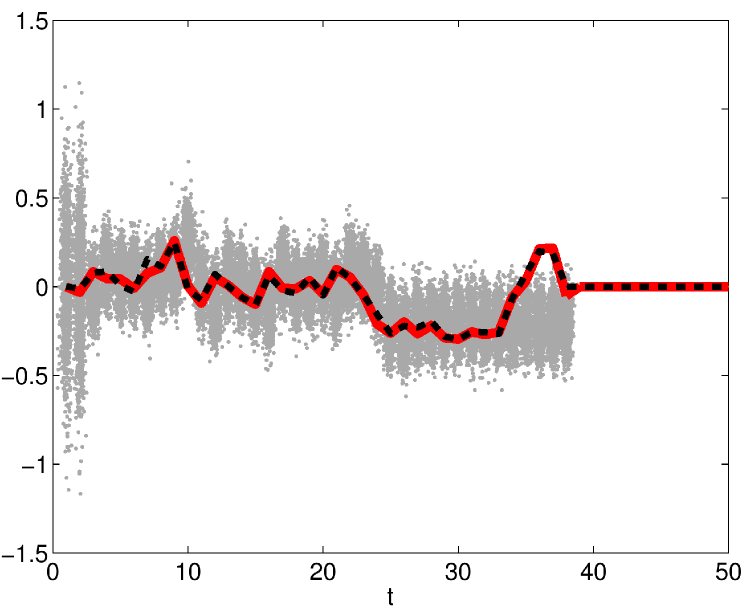
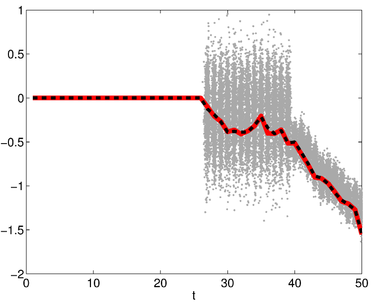
${\boldsymbol{s}}(0)$ was set to $0$ and changed (either an element added or removed) with probability 0.03. $a_{i},{\boldsymbol{b}}_{i},{\boldsymbol{Q}}_{i},i=1,\dots,N,$ were all generated from a unitary Gaussian distribution. The state dimension was set to $n=30$ and the measurement dimension to $20$. $M=10^{6}$, $\lambda=1$, $\Delta t=3$ and the system was simulated 50 time steps. The whole simulation, including NCPF, took less than half a minute on a standard laptop computer. Fig. 1 and 2 show, for a typical simulation, the true state (dashed lines) and the estimated (solid lines) expectation value of the state from the NCPF. State 1 was nonzero between $t=0$ and $t=38$. At time $t=26$ element 27 in the state was added to the support. As seen in the figure, the NCPF almost perfectly manage to track and detect the correct state elements as nonzero. Fig. 1 and 2 illustrate the particle densities for the first and 27th element of the state as it propagates over time.

Figure 1: An illustratration of the particle density of NCPF, the approximate expectation value of NCPF and the true first element of the state.

Figure 2: An illustratration of the particle density of NCPF, the approximate expectation value of NCPF and the true 27th element of the state.

We compare these results to that of a particle filter and to the result obtained by ignoring the temporal dependence between states and apply NLCS at each time instance.

V-A Particle Filter

It is well known that particle filter can not handle problems of too high dimension (the state dimension $n$ large). This is intuitively understood from the fact that each particle represent a hypotesis. As the dimension increase so does also the different directions the noise can disturb the state etc. The number of hypothesis needed can hence seen growing exponentially in the state dimension. The number of particles needed to handle a low dimensional system is therefore far fewer than for a high dimensional system.

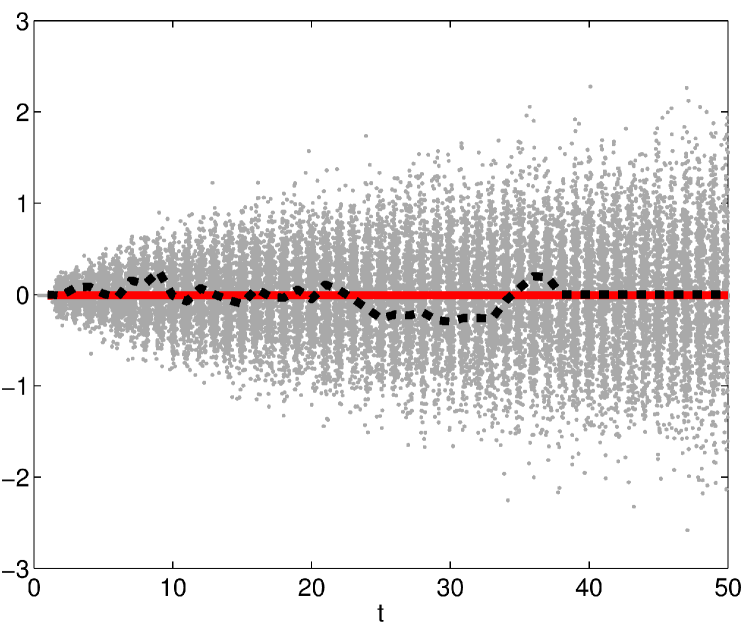
Here we apply the particle filter with $10^{6}$ particles to estimate the full 30 dimensional state. To be fair, we initialized the particles to the true state (the support of the true state at $t=1$ was given to the NCPF). The estimated expectation value for the first element in the state, the true trajectory of the first element in the state and a visualization of the particles are shown in Fig. 3. As seen, the particle filter totally fails to estimate the first element of the state. Neither does it succeed in giving a usable estimate for element 27.

Figure 3: The estimated expectation value of the first element in the state for the particle filter, the true trajectory of the first element in the state and a visualization of the particles’ first element.

V-B Nonlinear Compressive Sensing

NLCS can approximate the solution of problems of the form

$$\min_{{\boldsymbol{x}},{\boldsymbol{w}}} \|{\boldsymbol{x}}\|_{0}+\|{\boldsymbol{w}}\|_{\boldsymbol{R}}$$ (20)

subj. to $${\boldsymbol{y}}(t)=h({\boldsymbol{x}})+{\boldsymbol{w}}.$$

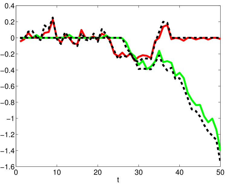
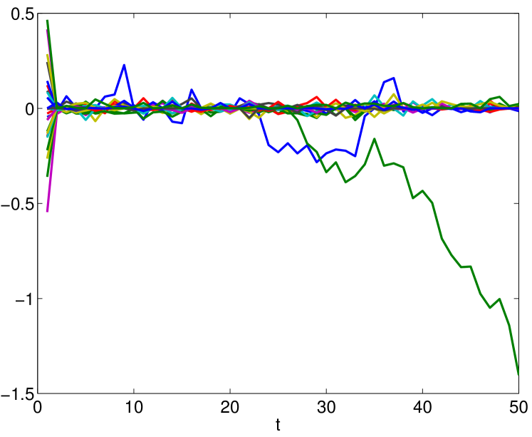
If we neglect the time dependence, and as a new ${\boldsymbol{y}}$ becomes available use (20) to find ${\boldsymbol{x}}(t)$, we get the results shown in Fig. 4. Dashed line shows the true first and 27th state element and the solid line, NLCS estimates of the first and 27th state element. Fig. 5 shows the full state estimates. As seen, NLCS gives comparable results with NCPF. However, the computational complexity is not comparable and while the NCPF took less than half a minute to run, the NLCS simulation took about 10 minutes.

Figure 4: Dashed line shows the true first and 27th state element and the solid line, NLCS estimates of the first and 27th state element.

Figure 5: An estiamte of ${\boldsymbol{x}}(t)$ using NLCS.

V-C Compressive Sensing and Some Remarks

We also applied ordinary linear compressive sensing to approximate the state. The result was worst than that shown above for the NLCS. This is maybe not that strange since ordinary compressive sensing neglects the quadratic part of the measurement equation. We also combined ordinary compressive sensing with the particle filter. This did not provide a satisfying result and compressive sensing often failed to detect the correct state to be added.

Last we want to add that the weakest part in NCPF is not the mechanism for adding or removing elements. The times we saw week performance, it was because the particle filter diverged.

VI Conclusion

This paper proposes Nonlinear Compressive Particle Filtering (NCPF), a novel combination of nonlinear compressive sensing and the particle filter. The proposed framework is shown to work better than nonlinear compressive sensing and particle filtering alone and offers an attractive solution to nonlinear sparse filtering.

References

- [1] J. Antonello, M. Verhaegen, R. Fraanje, T. van Werkhoven, H. C. Gerritsen, and C. U. Keller. Semidefinite programming for model-based sensorless adaptive optics. J. Opt. Soc. Am. A, 29(11):2428–2438, November 2012.
- [2] A. Beck and Y. C. Eldar. Sparsity constrained nonlinear optimization: Optimality conditions and algorithms. Technical Report arXiv:1203.4580, 2012.
- [3] T. Blumensath. Compressed sensing with nonlinear observations and related nonlinear optimization problems. Technical Report arXiv:1205.1650, 2012.
- [4] A. Bruckstein, D. Donoho, and M. Elad. From sparse solutions of systems of equations to sparse modeling of signals and images. SIAM Review, 51(1):34–81, 2009.
- [5] O. Bunk, A. Diaz, F. Pfeiffer, C. David, B. Schmitt, D. K. Satapathy, and J. F. van der Veen. Diffractive imaging for periodic samples: retrieving one-dimensional concentration profiles across microfluidic channels. Acta Crystallographica Section A, 63(4):306–314, July 2007.
- [6] E. Candès, J. Romberg, and T. Tao. Robust uncertainty principles: Exact signal reconstruction from highly incomplete frequency information. IEEE Transactions on Information Theory, 52:489–509, February 2006.
- [7] A. Carmi, P. Gurfil, and D. Kanevsky. Methods for sparse signal recovery using kalman filtering with embedded pseudo-measurement norms and quasi-norms. IEEE Transactions on Signal Processing, 58:2405 – 2409, April 2009.
- [8] F. Chernousko. Ellipsoidal state estimation for dynamical systems. Nonlinear analysis, 63:872–879, 2005.
- [9] J.V. Corbett. The pauli problem, state reconstruction and quantum-real numbers. Reports on Mathematical Physics, 57(1):53–68, 2006.
- [10] J.C. Dainty and J.R. Fienup. Phase retrieval and image reconstruction for astronomy. In editor H. Stark, editor, Image Recovery: Theory and Application. Academic Press, New York, 1987.
- [11] S. Das and N. Vaswani. PaFiMoCS: Particle Filtered Modified-CS and Applications in Visual Tracking across Illumination Change. Technical Report arXiv:1301.1374, Iowa State University, January 2013.
- [12] M. Dierolf, A. Menzel, P. Thibault, P. Schneider, C. M. Kewish, R. Wepf, O. Bunk, and F. Pfeiffer. Ptychographic x-ray computed tomography at the nanoscale. Nature, 467:436–439, 2010.
- [13] D. Donoho. Compressed sensing. IEEE Transactions on Information Theory, 52(4):1289–1306, April 2006.
- [14] Y. C. Eldar and G. Kutyniok. Compresed Sensing: Theory and Applications. Cambridge University Press, 2012.
- [15] J. R. Fienup, J. C. Marron, T. J. Schulz, and J. H. Seldin. Hubble space telescope characterized by using phase-retrieval algorithms. Applied Optics, 32(10):1747–1767, Apr 1993.
- [16] N. J. Gordon, D. J. Salmond, and A. F. M. Smith. Novel approach to nonlinear/non-Gaussian Bayesian state estimation. Radar and Signal Processing, IEE Proceedings F, 140(2):107–113, April 1993.
- [17] Simon J. Julier, Jeffery K. Uhlmann, and Hugh F. Durrant-Whyte. A new approach for filtering nonlinear systems. In American Control Conference, pages 1628–1632, 1995.
- [18] J. Miao, T. Ishikawa, Q. Shen, and T. Earnest. Extending x-ray crystallography to allow the imaging of noncrystalline materials, cells, and single protein complexes. Annual Review of Physical Chemistry, 59(1):387–410, 2008.
- [19] H. Ohlsson, A. Y. Yang, R. Dong, M. Verhaegen, and S. Sastry. Nonlinear Compressive Sensing. Technical Report arXiv, University of California, Berkeley, March 2013.
- [20] H. Ohlsson, A. Y. Yang, R. Dong, M. Verhaegen, and S. S. Sastry. Quadratic basis pursuit. CoRR, abs/1301.7002, 2013.
- [21] G. Rigatos. Derivative Free Nonlinear Kalman Filtering for MIMO Dynamical Systems: Application to Multi DOF Robotic Manipulators. International Journal of Advanced Robotic Systems, 8:47–61, 2011.
- [22] E. Scholte and M.E Campbell. A nonlinear set membership filter for on line applications. International Journal of Robust and Nonlinear Control, 13:1337–1358, 2003.
- [23] H.W. Sorenson. Kalman Filtering: Theory and Application. IEEE Press, 1985.
- [24] A. Szameit, Y. Shechtman, E. Osherovich, E. Bullkich, P. Sidorenko, H. Dana, S. Steiner, E. B. Kley, S. Gazit, T. Cohen-Hyams, S. Shoham, M. Zibulevsky, I. Yavneh, Y. C. Eldar, O. Cohen, and M. Segev. Sparsity-based single-shot subwavelength coherent diffractive imaging. Nature Materials, 11(5):455–459, May 2012.
- [25] N. Vaswani. Kalman filtered compressed sensing. Technical Report arXiv:0804.0819v1, Iowa State University, 2008.
- [26] N. Vaswani. Particle Filtering for Large-Dimensional State Spaces With Multimodal Observation Likelihoods. IEEE Trans. on Signal Processing, 56(10), October 2008.
- [27] A. Walther. The question of phase retrieval in optics. Optica Acta, 10:41–49, 1963.
- [28] E. Wang, J. Sliva, and L. Carin. Compressive particle filtering for target tracking. In Proceedings of the 15-th Workshop on Statistical Signal Processing, pages 233–236, 2009.