First order least squares method with weakly imposed boundary condition for convection dominated diffusion problems

Huangxin Chen School of Mathematical Sciences, Xiamen University, Xiamen, 361005, People’s Republic of China chx@xmu.edu.cn Guosheng Fu School of Mathematics, University of Minnesota, Minneapolis, MN 55455, USA fuxxx165@math.umn.edu Jingzhi Li Department of Financial Mathematics and Financial Engineering, South University of Science and Technology of China, Shenzhen, 518055, People’s Republic of China li.jz@sustc.edu.cn  and  Weifeng Qiu Department of Mathematics, City University of Hong Kong, 83 Tat Chee Avenue, Kowloon, Hong Kong, China weifeqiu@cityu.edu.hk
Abstract.

We present and analyze a first order least squares method for convection dominated diffusion problems, which provides robust L2superscript𝐿2L^{2} a priori error estimate for the scalar variable even if the given data fL2(Ω)𝑓superscript𝐿2Ωf\in L^{2}(\Omega). The novel theoretical approach is to rewrite the method in the framework of discontinuous Petrov–-Galerkin (DPG) method, and then show numerical stability by using a key equation discovered by J. Gopalakrishnan and W. Qiu [Math. Comp. 83(2014), pp. 537-552]. This new approach gives an alternative way to do numerical analysis for least squares methods for a large class of differential equations. We also show that the condition number of the global matrix is independent of the diffusion coefficient. A key feature of the method is that there is no stabilization parameter chosen empirically. In addition, Dirichlet boundary condition is weakly imposed. Numerical experiments verify our theoretical results and, in particular, show our way of weakly imposing Dirichlet boundary condition is essential to the design of least squares methods - numerical solutions on subdomains away from interior layers or boundary layers have remarkable accuracy even on coarse meshes, which are unstructured quasi-uniform.

Key words and phrases:
error estimate; least squares method; DPG method; convection diffusion problems.
2000 Mathematics Subject Classification:
65N30, 65L12, 35L15
Corresponding author: Weifeng Qiu

1. Introduction

In this paper, we present a robust a priori analysis of first order least squares method with weakly imposed boundary condition for the following convection dominated diffusion equation

ϵΔu+𝜷u+cu=italic-ϵΔ𝑢𝜷𝑢𝑐𝑢absent\displaystyle-\epsilon\Delta u+\boldsymbol{\beta}\cdot\nabla u+cu= f in Ω,𝑓 in Ω,\displaystyle\;f\quad\text{ in $\Omega$, } (1.1a)
u=𝑢absent\displaystyle u= g on Ω,𝑔 on Ω,\displaystyle\;g\quad\text{ on $\partial\Omega$, } (1.1b)

where ΩRdΩsuperscript𝑅𝑑\Omega\in R^{d} (d=2,3𝑑23d=2,3) is a polyhedral domain, 0<ϵ10italic-ϵ10<\epsilon\leq 1, c𝑐c a function in L(Ω)superscript𝐿ΩL^{\infty}(\Omega), f𝑓f a function in L2(Ω)superscript𝐿2ΩL^{2}(\Omega) and g𝑔g a function in H1/2(Ω)superscript𝐻12ΩH^{1/2}(\partial\Omega). Here, the variable flux 𝜷𝜷\boldsymbol{\beta} satisfies the following assumption:

𝜷ψb0>0 in Ω, for some function ψW1,(Ω),formulae-sequence𝜷𝜓subscript𝑏00 in Ω for some function 𝜓superscript𝑊1Ω\displaystyle\boldsymbol{\beta}\cdot\nabla\psi\geq b_{0}>0\text{ in }\Omega,\text{ for some function }\psi\in W^{1,\infty}(\Omega), (1.2a)
c12𝜷0 in Ω.𝑐12𝜷0 in Ω\displaystyle c-\frac{1}{2}\nabla\cdot\boldsymbol{\beta}\geq 0\text{ in }\Omega. (1.2b)

According to [1], the assumption (1.2a) is satisfied if

𝜷 has no closed curves and |𝜷(x)|0 for all xΩ.𝜷 has no closed curves and 𝜷𝑥0 for all 𝑥Ω\displaystyle\boldsymbol{\beta}\text{ has no closed curves and }|\boldsymbol{\beta}(x)|\neq 0\text{ for all }x\in\Omega.

Least squares methods have been frequently used to simulate solutions of partial differential equations arising from fluid dynamics and continuum mechanics. We refer to [7, 43] for comprehensive summary. It is well known that least squares methods have the following desirable features: it leads to a minimization problem; its numerical stability is not sensitive to the choice of finite element space or meshes; the resulting global stiffness matrices are symmetric and positive definite; a practical a posteriori error estimator can be given without any additional cost, and so on (see [5, 6, 14, 15, 17, 16, 18, 21, 22, 23, 26, 37, 48]).

Unfortunately, primitive least squares methods for convection dominated diffusion problems (1.1) have the following drawbacks. Firstly, if the term c12𝜷𝑐12𝜷c-\frac{1}{2}\nabla\cdot\boldsymbol{\beta} is not uniformly bounded from below by a positive constant, L2superscript𝐿2L^{2} a priori error estimate of primitive least squares methods will deteriorate as the diffusion coefficient ϵitalic-ϵ\epsilon goes to zero, even when the exact solution has no interior layers or boundary layers (see error estimates in [19, 41, 45]). Secondly, primitive least squares methods show a very poor performance for convection diffusion problem (1.1) with a sufficiently small diffusion coefficient, because large spurious oscillations are observed (see numerical experiments in [41]). We notice that in [41], residual-free bubble strategy is used to address the second drawback. But, the least squares method in [41] needs to compute basis functions element-wisely, which is relatively not easy to implement.

It is well known that streamline diffusion method [10], residual free bubble methods [8, 9, 13], and DG methods [1, 40, 42, 32, 33] do not suffer from the above two drawbacks of primitive least squares methods. We refer to [50, 52] as comprehensive summaries of numerical methods suitable for convection dominated diffusion problems. We would like to emphasize that none of these numerical methods (streamline diffusion method, residual free bubble methods, DG methods) results in symmetric global stiffness matrices. Hence from the point of view of solver design, the least squares method is more attractive than the other methods mentioned before and many works have been contributed to this subject (e.g. [16, 46]). Moreover, we derive that the condition number of linear system from our first order least squares method is at most 𝒪(h2)𝒪superscript2\mathcal{O}(h^{-2}), where hh is the mesh size. In particular, the condition number is independent of the diffusion coefficient. This property is important for designing efficient solver, e.g., multilevel method, for the first order least squares approximation of convection dominated diffusion equation.

In this paper, we propose and analyze our first order least squares method to address these two drawbacks for primitive least squares methods. In fact, it is difficult to provide robust L2superscript𝐿2L^{2} error estimate by the traditional approach of numerical analysis for least squares methods in [7]. So, it is necessary to look for an alternative approach. We notice that a weighted test function was used in [44] to obtain the L2superscript𝐿2L^{2} stability of the original DG method [49] for the transportation reaction equation, and this idea was generalized to convection-diffusion-reaction equation in [1] using the IP–DG methods. In this paper, we rewrite our method in the framework of discontinuous Petrov–-Galerkin (DPG) method, then show numerical stability by using a key equation discovered in [39]. The advantage of this new approach is that the weight function in [1] is shown to stay in some “equivalent” test function space (see (3.7) in section 3) such that numerical stability can be obtained without using any projection as in [1]. This approach is novel and useful to numerical analysis of least squares methods for a large class of differential equations. This new approach of numerical analysis is also different from traditional ones used for DPG method in [11, 27, 28, 29, 30]. We show that, roughly speaking, using polynomials of degree k+11𝑘11k+1\geq 1,

uhuL2(Ω)+ϵ1/2(uuh)L2(Ω)Chk+1uHk+2(Ω);subscriptnormsubscript𝑢𝑢superscript𝐿2Ωsuperscriptitalic-ϵ12subscriptnorm𝑢subscript𝑢superscript𝐿2Ω𝐶superscript𝑘1subscriptnorm𝑢superscript𝐻𝑘2Ω\|u_{h}-u\|_{L^{2}(\Omega)}+\epsilon^{1/2}\|\nabla(u-u_{h})\|_{L^{2}(\Omega)}\leq Ch^{k+1}\|u\|_{H^{k+2}(\Omega)}; (1.3)

if ϵ1/2hKsuperscriptitalic-ϵ12subscript𝐾\epsilon^{1/2}\leq h_{K} for any K𝒯h𝐾subscript𝒯K\in\mathcal{T}_{h},

uuhL2(Ω)+ϵ1/2(uuh)L2(Ω)+𝜷(uuh)L2(Ω)subscriptnorm𝑢subscript𝑢superscript𝐿2Ωsuperscriptitalic-ϵ12subscriptnorm𝑢subscript𝑢superscript𝐿2Ωsubscriptnorm𝜷𝑢subscript𝑢superscript𝐿2Ω\displaystyle\|u-u_{h}\|_{L^{2}(\Omega)}+\epsilon^{1/2}\|\nabla(u-u_{h})\|_{L^{2}(\Omega)}+\|\boldsymbol{\beta}\cdot\nabla(u-u_{h})\|_{L^{2}(\Omega)}
\displaystyle\leq Chk+1uHk+2(Ω).𝐶superscript𝑘1subscriptnorm𝑢superscript𝐻𝑘2Ω\displaystyle Ch^{k+1}\|u\|_{H^{k+2}(\Omega)}.

Here, the constant C𝐶C is independent of ϵitalic-ϵ\epsilon. Thus, we can conclude that a priori error estimate in (1.3) is robust with respect to the diffusion coefficient ϵitalic-ϵ\epsilon, which addresses the first draw back. We also want to emphasize that the convergence result (1.3) shows our method has L2superscript𝐿2L^{2} convergence rate even if fL2(Ω)𝑓superscript𝐿2Ωf\in L^{2}(\Omega), which means our method does not have excessive smoothness requirements than other methods. In order to overcome the second drawback, we impose Dirichlet boundary condition in an weak way, such that the error along the boundary layers will not propagate into the whole domain. We show the advantage of imposing boundary condition weakly by numerical experiments. We notice that our way of imposing boundary condition is similar to the weak imposition of Dirichlet boundary condition in [12, 2, 51], which belongs to Nitsche’s method in [47]. However, we do not have to choose any penalty terms empirically while [2] needs. We would like to emphasize that weakly imposing boundary condition is essential to least squares methods while it is incrementally helpful to streamline diffusion method and DG methods (see numerical experiments in [2]). If boundary condition is imposed strongly, the numerical solutions produced by streamline diffusion method and DG methods may have artificial oscillation along boundary layers, while the accuracy in subdomains away from boundary layers is still remarkable. However, according to our numerical experiments, if we impose boundary condition strongly, then numerical solution of least squares methods will be polluted on almost the whole domain by boundary layers. We have tried to add several stabilization terms, which have been utilized by streamline diffusion method or DG methods, into least squares methods to prevent propagation of error from boundary layers. None of them works except weakly imposing boundary condition.

This paper is the first one which addresses the two drawbacks of least squares methods for convection dominated diffusion problems. Now, we would like to compare with DPG methods, which can be considered as a special class of least squares methods. We notice that all DPG methods [3, 20, 31] need to compute optimal test function space. on each element such that the implementation is more complicated than ours (Methods in [24, 25] are similar to DPG methods.) Next, we would like to compare our results with IP–DG method [1]. [1] is the first paper which gives robust a priori error estimate for variable flux 𝜷𝜷\boldsymbol{\beta}. However, IP–DG method [1] has to choose stabilization parameter empirically while our method does not. In addition, IP–DG method [1] can have robust L2superscript𝐿2L^{2} convergence only when the mesh size h<h0subscript0h<h_{0} where h0subscript0h_{0} is a positive constant depending on 𝜷𝜷\boldsymbol{\beta} (see Theorem 4.44.44.4 in [1]). On the contrast, the convergence result of our method does not have this restriction.

The remainder of this paper is organized as follows. In section 222, we introduce our first order least squares method and the main theoretical results. In section 333, we show a novel approach to do numerical analysis for least squares methods (not restricted to our first order least squares method for convection dominated diffusion problems). In section 444, we prove a priori error estimates by using the approach introduced in section 333. In section 555, we prove the estimate of condition number of global stiffness matrix provided by our method. In section 666, we give numerical experiments which verify our theoretical results. In section 777, we extend our first order least squares method for transportation reaction problems.

2. First order least squares method and main theoretical result

In this section, we present setting of meshes, first order least squares method and the main theoretical results.

2.1. Setting of meshes

Let 𝒯h={K}subscript𝒯𝐾\mathcal{T}_{h}=\{K\} be a conforming triangulation of the domain ΩΩ\Omega made of shape-regular simplexes K𝐾K. For each element K𝒯h𝐾subscript𝒯K\in\mathcal{T}_{h}, we set hK:=|K|1dassignsubscript𝐾superscript𝐾1𝑑h_{K}:=|K|^{\frac{1}{d}} and for each of its faces e𝑒e, hF:=|F|1d1assignsubscript𝐹superscript𝐹1𝑑1h_{F}:=|F|^{\frac{1}{d-1}}, where |||\cdot| denotes the Lebesgue measure in d𝑑d or d1𝑑1d-1 dimensions. We associate to 𝒯hsubscript𝒯\mathcal{T}_{h} the set of faces hsubscript\mathcal{E}_{h} as well as those of interior faces hisubscriptsuperscript𝑖\mathcal{E}^{i}_{h} and boundary faces hsuperscriptsubscript\mathcal{E}_{h}^{\partial}. We say that Fhi𝐹subscriptsuperscript𝑖F\in\mathcal{E}^{i}_{h} if there are two elements K+superscript𝐾K^{+} and Ksuperscript𝐾K^{-} in 𝒯hsubscript𝒯\mathcal{T}_{h} such that F=K+K𝐹superscript𝐾superscript𝐾F=\partial K^{+}\cap\partial K^{-}, and we say that Fh𝐹superscriptsubscriptF\in\mathcal{E}_{h}^{\partial} if there is an element K𝐾K in 𝒯hsubscript𝒯\mathcal{T}_{h} such that F=KΩ𝐹𝐾ΩF=\partial K\cap\partial\Omega. It is obvious that h=hihsubscriptsuperscriptsubscript𝑖superscriptsubscript\mathcal{E}_{h}=\mathcal{E}_{h}^{i}\cup\mathcal{E}_{h}^{\partial}.

2.2. First order least squares method

We define 𝒒=ϵ1/2u𝒒superscriptitalic-ϵ12𝑢\boldsymbol{q}=-\epsilon^{1/2}\nabla u. We can rewrite (1.1) as the following first-order equations:

𝒒+ϵ1/2u𝒒superscriptitalic-ϵ12𝑢\displaystyle\boldsymbol{q}+\epsilon^{1/2}\nabla u =0 in Ω,absent0 in Ω\displaystyle=0\text{ in }\Omega, (2.1a)
ϵ1/2𝒒+𝜷u+cusuperscriptitalic-ϵ12𝒒𝜷𝑢𝑐𝑢\displaystyle\epsilon^{1/2}\nabla\cdot\boldsymbol{q}+\boldsymbol{\beta}\cdot\nabla u+cu =f in Ω,absent𝑓 in Ω\displaystyle=f\text{ in }\Omega, (2.1b)
u𝑢\displaystyle u =g on Ω.absent𝑔 on Ω\displaystyle=g\text{ on }\partial\Omega. (2.1c)

We define the finite element space 𝒰h=𝑸h×Whsubscript𝒰subscript𝑸subscript𝑊\mathcal{U}_{h}=\boldsymbol{Q}_{h}\times W_{h}, where

𝑸hsubscript𝑸\displaystyle\boldsymbol{Q}_{h} ={𝒑H(div,Ω):𝒑|KPk+1(K;d)+𝒙Pk+1(K),K𝒯h},absentconditional-set𝒑𝐻divΩformulae-sequenceevaluated-at𝒑𝐾subscript𝑃𝑘1𝐾superscript𝑑𝒙subscript𝑃𝑘1𝐾for-all𝐾subscript𝒯\displaystyle=\{\boldsymbol{p}\in H(\text{div},\Omega):\boldsymbol{p}|_{K}\in P_{k+1}(K;\mathbb{R}^{d})+\boldsymbol{x}P_{k+1}(K),\quad\forall K\in\mathcal{T}_{h}\}, (2.2a)
Whsubscript𝑊\displaystyle W_{h} ={w|KH1(Ω):wPk+1(K),K𝒯h}.\displaystyle=\{w|_{K}\in H^{1}(\Omega):w\in P_{k+1}(K),\quad\forall K\in\mathcal{T}_{h}\}. (2.2b)

Here, Pk(D)subscript𝑃𝑘𝐷P_{k}(D) is the space of polynomials on the domain D𝐷D of total degree at most k𝑘k, a non-negative integer. Obviously, there is a positive constant C𝐶C,

𝒑𝒏KΩsubscriptnorm𝒑𝒏𝐾Ω\displaystyle\|\boldsymbol{p}\cdot\boldsymbol{n}\|_{\partial K\cap\partial\Omega} ChK1/2𝒑K,𝒑𝑸h,K𝒯h,formulae-sequenceabsent𝐶superscriptsubscript𝐾12subscriptnorm𝒑𝐾formulae-sequencefor-all𝒑subscript𝑸𝐾subscript𝒯\displaystyle\leq Ch_{K}^{-1/2}\|\boldsymbol{p}\|_{K},\quad\forall\boldsymbol{p}\in\boldsymbol{Q}_{h},K\in\mathcal{T}_{h}, (2.3a)
𝒑Ksubscriptnorm𝒑𝐾\displaystyle\|\nabla\cdot\boldsymbol{p}\|_{K} ChK1𝒑K,𝒑𝑸h,K𝒯h.formulae-sequenceabsent𝐶superscriptsubscript𝐾1subscriptnorm𝒑𝐾formulae-sequencefor-all𝒑subscript𝑸𝐾subscript𝒯\displaystyle\leq Ch_{K}^{-1}\|\boldsymbol{p}\|_{K},\quad\forall\boldsymbol{p}\in\boldsymbol{Q}_{h},K\in\mathcal{T}_{h}. (2.3b)

The first order least squares method is to find (𝒒h,uh)𝒰hsubscript𝒒subscript𝑢subscript𝒰(\boldsymbol{q}_{h},u_{h})\in\mathcal{U}_{h} satisfying

(𝒒h+ϵ1/2uh,𝒑+ϵ1/2w)Ωsubscriptsubscript𝒒superscriptitalic-ϵ12subscript𝑢𝒑superscriptitalic-ϵ12𝑤Ω\displaystyle\left(\boldsymbol{q}_{h}+\epsilon^{1/2}\nabla u_{h},\boldsymbol{p}+\epsilon^{1/2}\nabla w\right)_{\Omega} (2.4)
+(ϵ1/2𝒒h+𝜷uh+cuh,ϵ1/2𝒑+𝜷w+cw)Ωsubscriptsuperscriptitalic-ϵ12subscript𝒒𝜷subscript𝑢𝑐subscript𝑢superscriptitalic-ϵ12𝒑𝜷𝑤𝑐𝑤Ω\displaystyle\quad+\left(\epsilon^{1/2}\nabla\cdot\boldsymbol{q}_{h}+\boldsymbol{\beta}\cdot\nabla u_{h}+cu_{h},\epsilon^{1/2}\nabla\cdot\boldsymbol{p}+\boldsymbol{\beta}\cdot\nabla w+cw\right)_{\Omega}
+ΣFhhF1(ϵ+max(𝜷𝒏(x),0))uh,wFsubscriptΣ𝐹superscriptsubscriptsuperscriptsubscript𝐹1subscriptitalic-ϵ𝜷𝒏𝑥0subscript𝑢𝑤𝐹\displaystyle\quad+\Sigma_{F\in\mathcal{E}_{h}^{\partial}}h_{F}^{-1}\langle\left(\epsilon+\max(-\boldsymbol{\beta}\cdot\boldsymbol{n}(x),0)\right)u_{h},w\rangle_{F}
=\displaystyle= (f,ϵ1/2𝒑+𝜷w+cw)Ωsubscript𝑓superscriptitalic-ϵ12𝒑𝜷𝑤𝑐𝑤Ω\displaystyle(f,\epsilon^{1/2}\nabla\cdot\boldsymbol{p}+\boldsymbol{\beta}\cdot\nabla w+cw)_{\Omega}
+ΣFhhF1(ϵ+max(𝜷𝒏(x),0))g,wF,(𝒑,w)𝒰h.subscriptΣ𝐹superscriptsubscriptsuperscriptsubscript𝐹1subscriptitalic-ϵ𝜷𝒏𝑥0𝑔𝑤𝐹for-all𝒑𝑤subscript𝒰\displaystyle\quad+\Sigma_{F\in\mathcal{E}_{h}^{\partial}}h_{F}^{-1}\langle\left(\epsilon+\max(-\boldsymbol{\beta}\cdot\boldsymbol{n}(x),0)\right)g,w\rangle_{F},\quad\forall(\boldsymbol{p},w)\in\mathcal{U}_{h}.

In (2.4), the inner products are defined in the following natural manner:

(u,v)Ω=Ωuv𝑑x and u,vF=Fuv𝑑s,Fh,formulae-sequencesubscript𝑢𝑣ΩsubscriptΩ𝑢𝑣differential-d𝑥 and subscript𝑢𝑣𝐹subscript𝐹𝑢𝑣differential-d𝑠for-all𝐹subscript\displaystyle(u,v)_{\Omega}=\int_{\Omega}uvdx\text{ and }\langle u,v\rangle_{F}=\int_{F}uvds,\quad\forall F\in\mathcal{E}_{h},

with the obvious modifications for vector-valued functions.

Remark 2.1.

Notice that the boundary condition imposed on outflow boundary (Γ+={xΩ:𝜷𝒏(x)>0}superscriptΓconditional-set𝑥Ω𝜷𝒏𝑥0\Gamma^{+}=\{x\in\partial\Omega:\boldsymbol{\beta}\cdot\boldsymbol{n}(x)>0\}) is O(ϵ)𝑂italic-ϵO(\epsilon). This is the reason we say Dirichlet boundary condition is weakly imposed. If we ignore the weight function used in [19], the first order least squares method in [19] is to find (𝒒h,uh)𝒬h×Wg,hsubscript𝒒subscript𝑢subscript𝒬subscript𝑊𝑔(\boldsymbol{q}_{h},u_{h})\in\mathcal{Q}_{h}\times W_{g,h} satisfying

(𝒒h+ϵ1/2uh,𝒑+ϵ1/2w)Ωsubscriptsubscript𝒒superscriptitalic-ϵ12subscript𝑢𝒑superscriptitalic-ϵ12𝑤Ω\displaystyle\left(\boldsymbol{q}_{h}+\epsilon^{1/2}\nabla u_{h},\boldsymbol{p}+\epsilon^{1/2}\nabla w\right)_{\Omega} (2.5)
+(ϵ1/2𝒒h+𝜷uh+cuh,ϵ1/2𝒑+𝜷w+cw)Ωsubscriptsuperscriptitalic-ϵ12subscript𝒒𝜷subscript𝑢𝑐subscript𝑢superscriptitalic-ϵ12𝒑𝜷𝑤𝑐𝑤Ω\displaystyle\quad+\left(\epsilon^{1/2}\nabla\cdot\boldsymbol{q}_{h}+\boldsymbol{\beta}\cdot\nabla u_{h}+cu_{h},\epsilon^{1/2}\nabla\cdot\boldsymbol{p}+\boldsymbol{\beta}\cdot\nabla w+cw\right)_{\Omega}
=\displaystyle= (f,ϵ1/2𝒑+𝜷w+cw)Ω,(𝒑,w)𝒬h×W0,h,subscript𝑓superscriptitalic-ϵ12𝒑𝜷𝑤𝑐𝑤Ωfor-all𝒑𝑤subscript𝒬subscript𝑊0\displaystyle(f,\epsilon^{1/2}\nabla\cdot\boldsymbol{p}+\boldsymbol{\beta}\cdot\nabla w+cw)_{\Omega},\quad\forall(\boldsymbol{p},w)\in\mathcal{Q}_{h}\times W_{0,h},

where Wg,h={wWh:w|Ω=g}subscript𝑊𝑔conditional-set𝑤subscript𝑊evaluated-at𝑤Ω𝑔W_{g,h}=\{w\in W_{h}:w|_{\partial\Omega}=g\} and W0,h={wWh:w|Ω=0}subscript𝑊0conditional-set𝑤subscript𝑊evaluated-at𝑤Ω0W_{0,h}=\{w\in W_{h}:w|_{\partial\Omega}=0\}. The main difference between (2.4) and (2.5) is that in (2.5), Dirichlet boundary condition is imposed strongly while our method (2.4) uses weakly imposed boundary condition. Our convergence analysis in section 4 is also valid for least squares method (2.5). But, if the solution of (1.1) has boundary layers or interior layers, then our way of weakly imposing boundary condition in (2.4) can improve the accuracy of numerical solution in subdomains away from layers dramatically. We refer to section 555 for detailed description.

Remark 2.2.

In (2.4), we weakly imposed the Dirichlet boundary condition by

ΣFhhF1(ϵ+max(𝜷𝒏(x),0))uh,wF=ΣFhhF1(ϵ+max(𝜷𝒏(x),0))g,wF.subscriptΣ𝐹superscriptsubscriptsuperscriptsubscript𝐹1subscriptitalic-ϵ𝜷𝒏𝑥0subscript𝑢𝑤𝐹subscriptΣ𝐹superscriptsubscriptsuperscriptsubscript𝐹1subscriptitalic-ϵ𝜷𝒏𝑥0𝑔𝑤𝐹\displaystyle\Sigma_{F\in\mathcal{E}_{h}^{\partial}}h_{F}^{-1}\langle\left(\epsilon+\max(-\boldsymbol{\beta}\cdot\boldsymbol{n}(x),0)\right)u_{h},w\rangle_{F}=\Sigma_{F\in\mathcal{E}_{h}^{\partial}}h_{F}^{-1}\langle\left(\epsilon+\max(-\boldsymbol{\beta}\cdot\boldsymbol{n}(x),0)\right)g,w\rangle_{F}.

In fact, we can also weakly imposed the Dirichlet boundary condition as

ΣFh(hF1ϵ+max(𝜷𝒏(x),0))uh,wF=ΣFh(hF1ϵ+max(𝜷𝒏(x),0))g,wF.subscriptΣ𝐹superscriptsubscriptsubscriptsuperscriptsubscript𝐹1italic-ϵ𝜷𝒏𝑥0subscript𝑢𝑤𝐹subscriptΣ𝐹superscriptsubscriptsubscriptsuperscriptsubscript𝐹1italic-ϵ𝜷𝒏𝑥0𝑔𝑤𝐹\displaystyle\Sigma_{F\in\mathcal{E}_{h}^{\partial}}\langle\left(h_{F}^{-1}\epsilon+\max(-\boldsymbol{\beta}\cdot\boldsymbol{n}(x),0)\right)u_{h},w\rangle_{F}=\Sigma_{F\in\mathcal{E}_{h}^{\partial}}\langle\left(h_{F}^{-1}\epsilon+\max(-\boldsymbol{\beta}\cdot\boldsymbol{n}(x),0)\right)g,w\rangle_{F}.

Then, the first order least squares method is to find (𝒒h,uh)𝒰hsubscript𝒒subscript𝑢subscript𝒰(\boldsymbol{q}_{h},u_{h})\in\mathcal{U}_{h} satisfying

(𝒒h+ϵ1/2uh,𝒑+ϵ1/2w)Ωsubscriptsubscript𝒒superscriptitalic-ϵ12subscript𝑢𝒑superscriptitalic-ϵ12𝑤Ω\displaystyle\left(\boldsymbol{q}_{h}+\epsilon^{1/2}\nabla u_{h},\boldsymbol{p}+\epsilon^{1/2}\nabla w\right)_{\Omega} (2.6)
+(ϵ1/2𝒒h+𝜷uh+cuh,ϵ1/2𝒑+𝜷w+cw)Ωsubscriptsuperscriptitalic-ϵ12subscript𝒒𝜷subscript𝑢𝑐subscript𝑢superscriptitalic-ϵ12𝒑𝜷𝑤𝑐𝑤Ω\displaystyle\quad+\left(\epsilon^{1/2}\nabla\cdot\boldsymbol{q}_{h}+\boldsymbol{\beta}\cdot\nabla u_{h}+cu_{h},\epsilon^{1/2}\nabla\cdot\boldsymbol{p}+\boldsymbol{\beta}\cdot\nabla w+cw\right)_{\Omega}
+ΣFh(hF1ϵ+max(𝜷𝒏(x),0))uh,wFsubscriptΣ𝐹superscriptsubscriptsubscriptsuperscriptsubscript𝐹1italic-ϵ𝜷𝒏𝑥0subscript𝑢𝑤𝐹\displaystyle\quad+\Sigma_{F\in\mathcal{E}_{h}^{\partial}}\langle\left(h_{F}^{-1}\epsilon+\max(-\boldsymbol{\beta}\cdot\boldsymbol{n}(x),0)\right)u_{h},w\rangle_{F}
=\displaystyle= (f,ϵ1/2𝒑+𝜷w+cw)Ωsubscript𝑓superscriptitalic-ϵ12𝒑𝜷𝑤𝑐𝑤Ω\displaystyle(f,\epsilon^{1/2}\nabla\cdot\boldsymbol{p}+\boldsymbol{\beta}\cdot\nabla w+cw)_{\Omega}
+ΣFh(hF1ϵ+max(𝜷𝒏(x),0))g,wF,(𝒑,w)𝒰h.subscriptΣ𝐹superscriptsubscriptsubscriptsuperscriptsubscript𝐹1italic-ϵ𝜷𝒏𝑥0𝑔𝑤𝐹for-all𝒑𝑤subscript𝒰\displaystyle\quad+\Sigma_{F\in\mathcal{E}_{h}^{\partial}}\langle\left(h_{F}^{-1}\epsilon+\max(-\boldsymbol{\beta}\cdot\boldsymbol{n}(x),0)\right)g,w\rangle_{F},\quad\forall(\boldsymbol{p},w)\in\mathcal{U}_{h}.

We can still obtain the stability estimate similar to Lemma 4.1. However, the L2superscript𝐿2L^{2} convergence rate of (2.6) is the same as that of (2.4), since the approximation to 𝜷u𝜷𝑢\boldsymbol{\beta}\cdot\nabla u in L2superscript𝐿2L^{2}-norm gets involved with the error analysis (see the proof of Theorem 2.3).

2.3. Main theoretical results

We state our main theoretical results on a priori error analysis and condition number estimation of the first order least squares method as the following Theorems.

We denote by C𝐶C a positive constant, which is independent of ϵitalic-ϵ\epsilon and hh. We assume the assumptions (1.2) on 𝜷𝜷\boldsymbol{\beta} and c𝑐c hold.

Theorem 2.3.
uuhL2(Ω)+ϵ1/2(uuh)L2(Ω)Chk(ϵ+h)uHk+2(Ω).subscriptnorm𝑢subscript𝑢superscript𝐿2Ωsuperscriptitalic-ϵ12subscriptnorm𝑢subscript𝑢superscript𝐿2Ω𝐶superscript𝑘italic-ϵsubscriptnorm𝑢superscript𝐻𝑘2Ω\displaystyle\|u-u_{h}\|_{L^{2}(\Omega)}+\epsilon^{1/2}\|\nabla(u-u_{h})\|_{L^{2}(\Omega)}\leq Ch^{k}(\epsilon+h)\|u\|_{H^{k+2}(\Omega)}. (2.7)

In addition, if we further assume 𝛃W2,(𝒯h)𝛃superscript𝑊2subscript𝒯\boldsymbol{\beta}\in W^{2,\infty}(\mathcal{T}_{h}) and cW1,(𝒯h)𝑐superscript𝑊1subscript𝒯c\in W^{1,\infty}(\mathcal{T}_{h}),

uuhL2(Ω)+ϵ1/2(uuh)L2(Ω)Chk+1uHk+2(Ω).subscriptnorm𝑢subscript𝑢superscript𝐿2Ωsuperscriptitalic-ϵ12subscriptnorm𝑢subscript𝑢superscript𝐿2Ω𝐶superscript𝑘1subscriptnorm𝑢superscript𝐻𝑘2Ω\displaystyle\|u-u_{h}\|_{L^{2}(\Omega)}+\epsilon^{1/2}\|\nabla(u-u_{h})\|_{L^{2}(\Omega)}\leq Ch^{k+1}\|u\|_{H^{k+2}(\Omega)}. (2.8)
Theorem 2.4.

If 0<ϵ1/2hK0superscriptitalic-ϵ12subscript𝐾0<\epsilon^{1/2}\leq h_{K} for any K𝒯h𝐾subscript𝒯K\in\mathcal{T}_{h},

uuhL2(Ω)+ϵ1/2(uuh)L2(Ω)+𝜷(uuh)L2(Ω)subscriptnorm𝑢subscript𝑢superscript𝐿2Ωsuperscriptitalic-ϵ12subscriptnorm𝑢subscript𝑢superscript𝐿2Ωsubscriptnorm𝜷𝑢subscript𝑢superscript𝐿2Ω\displaystyle\|u-u_{h}\|_{L^{2}(\Omega)}+\epsilon^{1/2}\|\nabla(u-u_{h})\|_{L^{2}(\Omega)}+\|\boldsymbol{\beta}\cdot\nabla(u-u_{h})\|_{L^{2}(\Omega)} (2.9)
\displaystyle\leq Chk(ϵ+h)uHk+2(Ω).𝐶superscript𝑘italic-ϵsubscriptnorm𝑢superscript𝐻𝑘2Ω\displaystyle Ch^{k}(\epsilon+h)\|u\|_{H^{k+2}(\Omega)}.

In addition, if we further assume 𝛃W2,(𝒯h)𝛃superscript𝑊2subscript𝒯\boldsymbol{\beta}\in W^{2,\infty}(\mathcal{T}_{h}) and cW1,(𝒯h)𝑐superscript𝑊1subscript𝒯c\in W^{1,\infty}(\mathcal{T}_{h}),

uuhL2(Ω)+ϵ1/2(uuh)L2(Ω)+𝜷(uuh)L2(Ω)subscriptnorm𝑢subscript𝑢superscript𝐿2Ωsuperscriptitalic-ϵ12subscriptnorm𝑢subscript𝑢superscript𝐿2Ωsubscriptnorm𝜷𝑢subscript𝑢superscript𝐿2Ω\displaystyle\|u-u_{h}\|_{L^{2}(\Omega)}+\epsilon^{1/2}\|\nabla(u-u_{h})\|_{L^{2}(\Omega)}+\|\boldsymbol{\beta}\cdot\nabla(u-u_{h})\|_{L^{2}(\Omega)} (2.10)
\displaystyle\leq Chk+1uHk+2(Ω).𝐶superscript𝑘1subscriptnorm𝑢superscript𝐻𝑘2Ω\displaystyle Ch^{k+1}\|u\|_{H^{k+2}(\Omega)}.
Theorem 2.5.

We denote by κ𝜅\kappa the condition number of global stiffness matrix of first order least squares method (2.4). If we assume the meshes are quasi-uniform, then

κCh2.𝜅𝐶superscript2\displaystyle\kappa\leq Ch^{-2}. (2.11)
Remark 2.6.

In Theorem 2.4, we obtain optimal convergence of uuhL2(Ω)+ϵ1/2(uuh)L2(Ω)+𝜷(uuh)L2(Ω)subscriptnorm𝑢subscript𝑢superscript𝐿2Ωsuperscriptitalic-ϵ12subscriptnorm𝑢subscript𝑢superscript𝐿2Ωsubscriptnorm𝜷𝑢subscript𝑢superscript𝐿2Ω\|u-u_{h}\|_{L^{2}(\Omega)}+\epsilon^{1/2}\|\nabla(u-u_{h})\|_{L^{2}(\Omega)}+\|\boldsymbol{\beta}\cdot\nabla(u-u_{h})\|_{L^{2}(\Omega)} if 0<ϵ1/2hK0superscriptitalic-ϵ12subscript𝐾0<\epsilon^{1/2}\leq h_{K} for any K𝒯h𝐾subscript𝒯K\in\mathcal{T}_{h}. The restriction on mesh size is due to the energy norm of 𝒰𝒰\mathcal{U} in Lemma 4.1 is

(𝒑,w)𝒰2=superscriptsubscriptnorm𝒑𝑤𝒰2absent\displaystyle\|(\boldsymbol{p},w)\|_{\mathcal{U}}^{2}= wL2(Ω)2+ϵwL2(Ω)2+wL2(Ω,𝜷)2+𝒑L2(Ω)2superscriptsubscriptnorm𝑤superscript𝐿2Ω2italic-ϵsuperscriptsubscriptnorm𝑤superscript𝐿2Ω2superscriptsubscriptnorm𝑤superscript𝐿2Ω𝜷2superscriptsubscriptnorm𝒑superscript𝐿2Ω2\displaystyle\|w\|_{L^{2}(\Omega)}^{2}+\epsilon\|\nabla w\|_{L^{2}(\Omega)}^{2}+\|w\|_{L^{2}(\partial\Omega,\boldsymbol{\beta})}^{2}+\|\boldsymbol{p}\|_{L^{2}(\Omega)}^{2}
+ϵ1/2𝒑+𝜷wL2(Ω)2,(𝒑,w)𝒰.superscriptsubscriptnormsuperscriptitalic-ϵ12𝒑𝜷𝑤superscript𝐿2Ω2for-all𝒑𝑤𝒰\displaystyle\quad+\|\epsilon^{1/2}\nabla\cdot\boldsymbol{p}+\boldsymbol{\beta}\cdot\nabla w\|_{L^{2}(\Omega)}^{2},\quad\forall(\boldsymbol{p},w)\in\mathcal{U}.

Thus, we need to utilize inverse inequality and the above restriction on mesh size to obtain upper bound on 𝜷(uuh)L2(Ω)subscriptnorm𝜷𝑢subscript𝑢superscript𝐿2Ω\|\boldsymbol{\beta}\cdot\nabla(u-u_{h})\|_{L^{2}(\Omega)}.

3. The approach to analysis

In this section, an alternative approach is introduced for numerical analysis of least squares methods in general (not restricted to the first order least squares method (2.4)). First of all, we show least squares methods and DPG method in abstract settings, respectively. Then, we rewrite least squares methods in the framework of DPG method. A key equation in [39] is then used to show how to achieve numerical stability of least squares methods.

Suppose we want to approximate solution 𝒰𝒰𝒰𝒰{\scriptstyle{\mathscr{U}}}\in\mathcal{U} satisfying

𝒰=f𝒱.𝒰𝑓𝒱\mathcal{L}{\scriptstyle{\mathscr{U}}}=f\in\mathcal{V}.

Here, 𝒰𝒰\mathcal{U} is a Banach space with norm 𝒰\|\cdot\|_{\mathcal{U}}, and 𝒱𝒱\mathcal{V} is a Hilbert space with norm 𝒱\|\cdot\|_{\mathcal{V}}. We assume that the linear operator \mathcal{L} is in 𝔹(𝒰,𝒱)𝔹𝒰𝒱\mathbb{B}(\mathcal{U},\mathcal{V}), which is the space of bounded linear operators from 𝒰𝒰\mathcal{U} to 𝒱𝒱\mathcal{V}. Then, least squares methods are to find 𝒰h𝒰hsubscript𝒰subscript𝒰{\scriptstyle{\mathscr{U}}}_{\!h}\in\mathcal{U}_{h} satisfying

(𝒰h,𝒲)𝒱=(f,𝒲)𝒱𝒲𝒰h.formulae-sequencesubscriptsubscript𝒰𝒲𝒱subscript𝑓𝒲𝒱for-all𝒲subscript𝒰(\mathcal{L}{\scriptstyle{\mathscr{U}}}_{\!h},\mathcal{L}{\scriptstyle{\mathscr{W}}})_{\mathcal{V}}=(f,\mathcal{L}{\scriptstyle{\mathscr{W}}})_{\mathcal{V}}\quad\forall{\scriptstyle{\mathscr{W}}}\in\mathcal{U}_{h}. (3.1)

Here, 𝒰hsubscript𝒰\mathcal{U}_{h} is a finite dimensional trial subspace of 𝒰𝒰\mathcal{U} (where hh denotes a parameter determining the finite dimension).

On the other hand, DPG method can be described in the following general context. Suppose we want to approximate 𝒰𝒰𝒰𝒰{\scriptstyle{\mathscr{U}}}\in\mathcal{U} satisfying

b(𝒰,𝒱)=l(𝒱),𝒱𝒱.formulae-sequence𝑏𝒰𝒱𝑙𝒱for-all𝒱𝒱b({\scriptstyle{\mathscr{U}}},{\scriptstyle{\mathscr{V}}})=l({\scriptstyle{\mathscr{V}}}),\quad\forall{\scriptstyle{\mathscr{V}}}\in\mathcal{V}. (3.2)

Here 𝒰𝒰\mathcal{U} is a Banach space with norm 𝒰\|\cdot\|_{\mathcal{U}} and 𝒱𝒱\mathcal{V} is a Hilbert space under an inner product (,)𝒱subscript𝒱(\cdot,\cdot)_{\mathcal{V}} with corresponding norm 𝒱\|\cdot\|_{\mathcal{V}}. We assume that the bi-linear form b(,):𝒰×𝒱:𝑏maps-to𝒰𝒱b(\cdot,\cdot):\mathcal{U}\times\mathcal{V}\mapsto\mathbb{R} is continuous and the linear form l():𝒱:𝑙maps-to𝒱l(\cdot):\mathcal{V}\mapsto\mathbb{R} is also continuous. Define T:𝒰𝒱:𝑇maps-to𝒰𝒱T:\mathcal{U}\mapsto\mathcal{V} by

(T𝒲,𝒱)𝒱=b(𝒲,𝒱),𝒱𝒱.formulae-sequencesubscript𝑇𝒲𝒱𝒱𝑏𝒲𝒱for-all𝒱𝒱(T{\scriptstyle{\mathscr{W}}},{\scriptstyle{\mathscr{V}}})_{\mathcal{V}}=b({\scriptstyle{\mathscr{W}}},{\scriptstyle{\mathscr{V}}}),\qquad\forall{\scriptstyle{\mathscr{V}}}\in\mathcal{V}. (3.3)

Then, the DPG approximation to 𝒰𝒰{\scriptstyle{\mathscr{U}}}, lies in a finite dimensional trial subspace 𝒰h𝒰subscript𝒰𝒰\mathcal{U}_{h}\subset\mathcal{U}. It satisfies

b(𝒰h,𝒱)=l(𝒱),𝒱𝒱h,formulae-sequence𝑏subscript𝒰𝒱𝑙𝒱for-all𝒱subscript𝒱b({\scriptstyle{\mathscr{U}}}_{\!h},{\scriptstyle{\mathscr{V}}})=l({\scriptstyle{\mathscr{V}}}),\quad\forall{\scriptstyle{\mathscr{V}}}\in\mathcal{V}_{h}, (3.4)

where 𝒱h=T(𝒰h)subscript𝒱𝑇subscript𝒰\mathcal{V}_{h}=T(\mathcal{U}_{h}). Since 𝒰h𝒱hsubscript𝒰subscript𝒱\mathcal{U}_{h}\neq\mathcal{V}_{h} in general, this is a Petrov-Galerkin approximation. The method (3.4) is the DPG method. The excellent stability and approximation properties of this method are well known [28, 29].

Now, we can rewrite the least squares methods (3.1) in the framework of DPG method in the following way. The corresponding DPG method is to find 𝒰h𝒰hsubscript𝒰subscript𝒰{\scriptstyle{\mathscr{U}}}_{\!h}\in\mathcal{U}_{h} such that

b(𝒰h,𝒱)=(f,𝒱)𝒱𝒱𝒱h=T(𝒰h),formulae-sequence𝑏subscript𝒰𝒱subscript𝑓𝒱𝒱for-all𝒱subscript𝒱𝑇subscript𝒰b({\scriptstyle{\mathscr{U}}}_{\!h},{\scriptstyle{\mathscr{V}}})=(f,{\scriptstyle{\mathscr{V}}})_{\mathcal{V}}\quad\forall{\scriptstyle{\mathscr{V}}}\in\mathcal{V}_{h}=T(\mathcal{U}_{h}), (3.5)

where the bi-linear form

b(𝒲,𝒱)=(𝒲,𝒱)𝒱,𝒲𝒰,𝒱𝒱.formulae-sequence𝑏𝒲𝒱subscript𝒲𝒱𝒱formulae-sequencefor-all𝒲𝒰𝒱𝒱b({\scriptstyle{\mathscr{W}}},{\scriptstyle{\mathscr{V}}})=(\mathcal{L}{\scriptstyle{\mathscr{W}}},{\scriptstyle{\mathscr{V}}})_{\mathcal{V}},\quad\forall{\scriptstyle{\mathscr{W}}}\in\mathcal{U},{\scriptstyle{\mathscr{V}}}\in\mathcal{V}.

Here, for any 𝒲𝒰𝒲𝒰{\scriptstyle{\mathscr{W}}}\in\mathcal{U},

(T𝒲,δ𝒱)𝒱=b(𝒲,δ𝒱)δ𝒱𝒱.formulae-sequencesubscript𝑇𝒲𝛿𝒱𝒱𝑏𝒲𝛿𝒱for-all𝛿𝒱𝒱(T{\scriptstyle{\mathscr{W}}},\delta{\scriptstyle{\mathscr{V}}})_{\mathcal{V}}=b({\scriptstyle{\mathscr{W}}},\delta{\scriptstyle{\mathscr{V}}})\quad\forall\delta{\scriptstyle{\mathscr{V}}}\in\mathcal{V}.

We say the corresponding DPG method (3.5) is numerical stable if there is a constant C𝐶C independent of mesh size hh, such that for any 𝒲𝒰h𝒲subscript𝒰{\scriptstyle{\mathscr{W}}}\in\mathcal{U}_{h},

𝒲𝒰Csup0𝒱𝒱hb(𝒲,𝒱)𝒱𝒱.subscriptnorm𝒲𝒰𝐶subscriptsupremum0𝒱subscript𝒱𝑏𝒲𝒱subscriptnorm𝒱𝒱\|{\scriptstyle{\mathscr{W}}}\|_{\mathcal{U}}\leq C\sup_{0\neq{\scriptstyle{\mathscr{V}}}\in\mathcal{V}_{h}}\dfrac{b({\scriptstyle{\mathscr{W}}},{\scriptstyle{\mathscr{V}}})}{\|{\scriptstyle{\mathscr{V}}}\|_{\mathcal{V}}}. (3.6)

In general, it is not easy to know what are elements in the finite dimensional space 𝒱hsubscript𝒱\mathcal{V}_{h}. So, it is usually not easy to estimate the right hand side of the inequality (3.6). But, according to the following Theorem 3.1, we have that for any 𝒲𝒰h𝒰𝒲subscript𝒰𝒰{\scriptstyle{\mathscr{W}}}\in\mathcal{U}_{h}\subset\mathcal{U},

sup0𝒱𝒱hb(𝒲,𝒱)𝒱𝒱=sup0𝒱𝒱b(𝒲,𝒱)𝒱𝒱.subscriptsupremum0𝒱subscript𝒱𝑏𝒲𝒱subscriptnorm𝒱𝒱subscriptsupremum0𝒱𝒱𝑏𝒲𝒱subscriptnorm𝒱𝒱\sup_{0\neq{\scriptstyle{\mathscr{V}}}\in\mathcal{V}_{h}}\dfrac{b({\scriptstyle{\mathscr{W}}},{\scriptstyle{\mathscr{V}}})}{\|{\scriptstyle{\mathscr{V}}}\|_{\mathcal{V}}}=\sup_{0\neq{\scriptstyle{\mathscr{V}}}\in\mathcal{V}}\dfrac{b({\scriptstyle{\mathscr{W}}},{\scriptstyle{\mathscr{V}}})}{\|{\scriptstyle{\mathscr{V}}}\|_{\mathcal{V}}}. (3.7)

(3.7) is the key equation discovered in work for DPG methods. We call 𝒱𝒱\mathcal{V} the “equivalent” test function space. By (3.7), in order to obtain (3.6), it is sufficient to achieve

𝒲𝒰Csup0𝒱𝒱b(𝒲,𝒱)𝒱𝒱.subscriptnorm𝒲𝒰𝐶subscriptsupremum0𝒱𝒱𝑏𝒲𝒱subscriptnorm𝒱𝒱\|{\scriptstyle{\mathscr{W}}}\|_{\mathcal{U}}\leq C\sup_{0\neq{\scriptstyle{\mathscr{V}}}\in\mathcal{V}}\dfrac{b({\scriptstyle{\mathscr{W}}},{\scriptstyle{\mathscr{V}}})}{\|{\scriptstyle{\mathscr{V}}}\|_{\mathcal{V}}}. (3.8)

The inequality (3.8) is usually easier to be obtained than (3.6). Notice that the least squares methods (3.1) is actually the same as the corresponding DPG method (3.5). This explains why it is relatively easier to obtain numerical stability of least squares methods. In fact, first order least squares methods based on first order Friedrichs’ systems in [34, 35, 36] can be shown to have numerical stability by using the key equation (3.7).

The proof of following Theorem 3.1 is included in that of Theorem 2.12.12.1 in [39]. In [39], the solution space 𝒰𝒰\mathcal{U} is restricted to Hilbert spaces. We put the proof here in order to make this paper more self-contained.

Theorem 3.1.

Let b:𝒰×𝒱:𝑏𝒰𝒱b:\mathcal{U}\times\mathcal{V}\rightarrow\mathbb{R} be a continuous bi-linear mapping. Here, 𝒰𝒰\mathcal{U} is a normed linear space, and 𝒱𝒱\mathcal{V} is a Hilbert space with associate norm 𝒱\|\cdot\|_{\mathcal{V}}.

We define a linear operator T:𝒰𝒱:𝑇maps-to𝒰𝒱T:\mathcal{U}\mapsto\mathcal{V} by

(T𝒲,δ𝒱)𝒱=b(𝒲,δ𝒱),δ𝒱𝒱.formulae-sequencesubscript𝑇𝒲𝛿𝒱𝒱𝑏𝒲𝛿𝒱for-all𝛿𝒱𝒱(T{\scriptstyle{\mathscr{W}}},\delta{\scriptstyle{\mathscr{V}}})_{\mathcal{V}}=b({\scriptstyle{\mathscr{W}}},\delta{\scriptstyle{\mathscr{V}}}),\quad\forall\delta{\scriptstyle{\mathscr{V}}}\in\mathcal{V}. (3.9)

Then, for any 𝒲𝒰𝒲𝒰{\scriptstyle{\mathscr{W}}}\in\mathcal{U}, we have that

sup0𝒱T(𝒰)b(𝒲,𝒱)𝒱𝒱=sup0𝒱𝒱b(𝒲,𝒱)𝒱𝒱.subscriptsupremum0𝒱𝑇𝒰𝑏𝒲𝒱subscriptnorm𝒱𝒱subscriptsupremum0𝒱𝒱𝑏𝒲𝒱subscriptnorm𝒱𝒱\sup_{0\neq{\scriptstyle{\mathscr{V}}}\in T(\mathcal{U})}\dfrac{b({\scriptstyle{\mathscr{W}}},{\scriptstyle{\mathscr{V}}})}{\|{\scriptstyle{\mathscr{V}}}\|_{\mathcal{V}}}=\sup_{0\neq{\scriptstyle{\mathscr{V}}}\in\mathcal{V}}\dfrac{b({\scriptstyle{\mathscr{W}}},{\scriptstyle{\mathscr{V}}})}{\|{\scriptstyle{\mathscr{V}}}\|_{\mathcal{V}}}. (3.10)
Proof.

Since the bi-linear mapping is continuous and 𝒱𝒱\mathcal{V} is a Hilbert space, the operator T𝑇T is well-defined.

We take 𝒲𝒰𝒲𝒰{\scriptstyle{\mathscr{W}}}\in\mathcal{U} arbitrarily. It is straightforward to see that

sup0𝒱T(𝒰)b(𝒲,𝒱)𝒱𝒱sup0𝒱𝒱b(𝒲,𝒱)𝒱𝒱,subscriptsupremum0𝒱𝑇𝒰𝑏𝒲𝒱subscriptnorm𝒱𝒱subscriptsupremum0𝒱𝒱𝑏𝒲𝒱subscriptnorm𝒱𝒱\sup_{0\neq{\scriptstyle{\mathscr{V}}}\in T(\mathcal{U})}\dfrac{b({\scriptstyle{\mathscr{W}}},{\scriptstyle{\mathscr{V}}})}{\|{\scriptstyle{\mathscr{V}}}\|_{\mathcal{V}}}\leq\sup_{0\neq{\scriptstyle{\mathscr{V}}}\in\mathcal{V}}\dfrac{b({\scriptstyle{\mathscr{W}}},{\scriptstyle{\mathscr{V}}})}{\|{\scriptstyle{\mathscr{V}}}\|_{\mathcal{V}}},

since T(𝒰)𝒱𝑇𝒰𝒱T(\mathcal{U})\subset\mathcal{V}.

If T𝒲=0𝒰𝑇𝒲0𝒰T{\scriptstyle{\mathscr{W}}}=0\in\mathcal{U}, then (3.10) is obviously true due to (3.9). If T𝒲0𝑇𝒲0T{\scriptstyle{\mathscr{W}}}\neq 0, then by (3.9) and the fact that 𝒱𝒱\mathcal{V} is a Hilbert space, we have

sup0𝒱𝒱b(𝒲,𝒱)𝒱𝒱=sup0𝒱𝒱(T𝒲,𝒱)𝒱𝒱𝒱=(T𝒲,T𝒲)𝒱T𝒲𝒱=b(𝒲,T𝒲)T𝒲𝒱sup0𝒱T(𝒰)b(𝒲,𝒱)𝒱𝒱.subscriptsupremum0𝒱𝒱𝑏𝒲𝒱subscriptnorm𝒱𝒱subscriptsupremum0𝒱𝒱subscript𝑇𝒲𝒱𝒱subscriptnorm𝒱𝒱subscript𝑇𝒲𝑇𝒲𝒱subscriptnorm𝑇𝒲𝒱𝑏𝒲𝑇𝒲subscriptnorm𝑇𝒲𝒱subscriptsupremum0𝒱𝑇𝒰𝑏𝒲𝒱subscriptnorm𝒱𝒱\sup_{0\neq{\scriptstyle{\mathscr{V}}}\in\mathcal{V}}\dfrac{b({\scriptstyle{\mathscr{W}}},{\scriptstyle{\mathscr{V}}})}{\|{\scriptstyle{\mathscr{V}}}\|_{\mathcal{V}}}=\sup_{0\neq{\scriptstyle{\mathscr{V}}}\in\mathcal{V}}\dfrac{(T{\scriptstyle{\mathscr{W}}},{\scriptstyle{\mathscr{V}}})_{\mathcal{V}}}{\|{\scriptstyle{\mathscr{V}}}\|_{\mathcal{V}}}=\dfrac{(T{\scriptstyle{\mathscr{W}}},T{\scriptstyle{\mathscr{W}}})_{\mathcal{V}}}{\|T{\scriptstyle{\mathscr{W}}}\|_{\mathcal{V}}}=\dfrac{b({\scriptstyle{\mathscr{W}}},T{\scriptstyle{\mathscr{W}}})}{\|T{\scriptstyle{\mathscr{W}}}\|_{\mathcal{V}}}\leq\sup_{0\neq{\scriptstyle{\mathscr{V}}}\in T(\mathcal{U})}\dfrac{b({\scriptstyle{\mathscr{W}}},{\scriptstyle{\mathscr{V}}})}{\|{\scriptstyle{\mathscr{V}}}\|_{\mathcal{V}}}.

We can conclude that for any 𝒲𝒰𝒲𝒰{\scriptstyle{\mathscr{W}}}\in\mathcal{U}, (3.10) is true. ∎

4. Convergence analysis

In this section, we shall prove Theorem 2.3 and Theorem 2.4. According to the approach of analysis in section 3, we rewrite first order least squares method (2.4) in the framework of DPG method. Then, we show the numerical stability of corresponding DPG method. Finally, we prove Theorem 2.3 and Theorem 2.4.

Throughout this section, we define 𝒰=H(div,Ω)×H1(Ω)𝒰𝐻divΩsuperscript𝐻1Ω\mathcal{U}=H(\text{div},\Omega)\times H^{1}(\Omega) and 𝒱=L2(Ω;d)×L2(Ω)×L2(Ω)𝒱superscript𝐿2Ωsuperscript𝑑superscript𝐿2Ωsuperscript𝐿2Ω\mathcal{V}=L^{2}(\Omega;\mathbb{R}^{d})\times L^{2}(\Omega)\times L^{2}(\partial\Omega). The inner product of 𝒱𝒱\mathcal{V} is defined by

((𝒓,v,μ),(δ𝒓,δv,δμ))𝒱subscript𝒓𝑣𝜇𝛿𝒓𝛿𝑣𝛿𝜇𝒱\displaystyle((\boldsymbol{r},v,\mu),(\delta\boldsymbol{r},\delta v,\delta\mu))_{\mathcal{V}} (4.1)
=\displaystyle= (𝒓,δ𝒓)Ω+(v,δv)Ω+ΣFhhF1(ϵ+max(𝜷𝒏(x),0))μ,δμF,subscript𝒓𝛿𝒓Ωsubscript𝑣𝛿𝑣ΩsubscriptΣ𝐹superscriptsubscriptsuperscriptsubscript𝐹1subscriptitalic-ϵ𝜷𝒏𝑥0𝜇𝛿𝜇𝐹\displaystyle(\boldsymbol{r},\delta\boldsymbol{r})_{\Omega}+(v,\delta v)_{\Omega}+\Sigma_{F\in\mathcal{E}_{h}^{\partial}}h_{F}^{-1}\langle\left(\epsilon+\max(-\boldsymbol{\beta}\cdot\boldsymbol{n}(x),0)\right)\mu,\delta\mu\rangle_{F},
(𝒓,v,μ),(δ𝒓,δv,δμ)𝒱.for-all𝒓𝑣𝜇𝛿𝒓𝛿𝑣𝛿𝜇𝒱\displaystyle\quad\forall(\boldsymbol{r},v,\mu),(\delta\boldsymbol{r},\delta v,\delta\mu)\in\mathcal{V}.

Obviously, 𝒱𝒱\mathcal{V} is a Hilbert space with respect to the inner product in (4.1). For any μL2(Ω)𝜇superscript𝐿2Ω\mu\in L^{2}(\partial\Omega), we define

μL2(Ω,𝜷)2=ΣFhhF1(ϵ+max(𝜷𝒏(x),0))1/2μL2(F)2.superscriptsubscriptnorm𝜇superscript𝐿2Ω𝜷2subscriptΣ𝐹superscriptsubscriptsuperscriptsubscript𝐹1superscriptsubscriptnormsuperscriptitalic-ϵ𝜷𝒏𝑥012𝜇superscript𝐿2𝐹2\|\mu\|_{L^{2}(\partial\Omega,\boldsymbol{\beta})}^{2}=\Sigma_{F\in\mathcal{E}_{h}^{\partial}}h_{F}^{-1}\|\left(\epsilon+\max(-\boldsymbol{\beta}\cdot\boldsymbol{n}(x),0)\right)^{1/2}\mu\|_{L^{2}(F)}^{2}. (4.2)

The norm of 𝒱𝒱\mathcal{V} is

(𝒓,v,μ)𝒱2=𝒓L2(Ω)2+vL2(Ω)2+μL2(Ω,𝜷)2,(𝒓,v,μ)𝒱.formulae-sequencesuperscriptsubscriptnorm𝒓𝑣𝜇𝒱2superscriptsubscriptnorm𝒓superscript𝐿2Ω2superscriptsubscriptnorm𝑣superscript𝐿2Ω2superscriptsubscriptnorm𝜇superscript𝐿2Ω𝜷2for-all𝒓𝑣𝜇𝒱\displaystyle\|(\boldsymbol{r},v,\mu)\|_{\mathcal{V}}^{2}=\|\boldsymbol{r}\|_{L^{2}(\Omega)}^{2}+\|v\|_{L^{2}(\Omega)}^{2}+\|\mu\|_{L^{2}(\partial\Omega,\boldsymbol{\beta})}^{2},\quad\forall(\boldsymbol{r},v,\mu)\in\mathcal{V}. (4.3)

The norm of 𝒰𝒰\mathcal{U} is defined by

(𝒑,w)𝒰2superscriptsubscriptnorm𝒑𝑤𝒰2\displaystyle\|(\boldsymbol{p},w)\|_{\mathcal{U}}^{2} (4.4)
=\displaystyle= wL2(Ω)2+ϵwL2(Ω)2+wL2(Ω,𝜷)2+𝒑L2(Ω)2superscriptsubscriptnorm𝑤superscript𝐿2Ω2italic-ϵsuperscriptsubscriptnorm𝑤superscript𝐿2Ω2superscriptsubscriptnorm𝑤superscript𝐿2Ω𝜷2superscriptsubscriptnorm𝒑superscript𝐿2Ω2\displaystyle\|w\|_{L^{2}(\Omega)}^{2}+\epsilon\|\nabla w\|_{L^{2}(\Omega)}^{2}+\|w\|_{L^{2}(\partial\Omega,\boldsymbol{\beta})}^{2}+\|\boldsymbol{p}\|_{L^{2}(\Omega)}^{2}
+ϵ1/2𝒑+𝜷wL2(Ω)2,(𝒑,w)𝒰.superscriptsubscriptnormsuperscriptitalic-ϵ12𝒑𝜷𝑤superscript𝐿2Ω2for-all𝒑𝑤𝒰\displaystyle\quad+\|\epsilon^{1/2}\nabla\cdot\boldsymbol{p}+\boldsymbol{\beta}\cdot\nabla w\|_{L^{2}(\Omega)}^{2},\quad\forall(\boldsymbol{p},w)\in\mathcal{U}.

4.1. Rewrite least squares method in DPG framework

The first order least squares method (2.4) is the same as the corresponding DPG method (4.5) in the following.

Equivalently, the first order least squares method (2.4) is to find (𝒒h,uh)𝒰hsubscript𝒒subscript𝑢subscript𝒰(\boldsymbol{q}_{h},u_{h})\in\mathcal{U}_{h} satisfying

b((𝒒h,uh),(𝒓,v,μ))𝑏subscript𝒒subscript𝑢𝒓𝑣𝜇\displaystyle b((\boldsymbol{q}_{h},u_{h}),(\boldsymbol{r},v,\mu)) (4.5)
=\displaystyle= (f,v)Ω+ΣFhhF1(ϵ+max(𝜷𝒏(x),0))g,μF,subscript𝑓𝑣ΩsubscriptΣ𝐹superscriptsubscriptsuperscriptsubscript𝐹1subscriptitalic-ϵ𝜷𝒏𝑥0𝑔𝜇𝐹\displaystyle(f,v)_{\Omega}+\Sigma_{F\in\mathcal{E}_{h}^{\partial}}h_{F}^{-1}\langle\left(\epsilon+\max(-\boldsymbol{\beta}\cdot\boldsymbol{n}(x),0)\right)g,\mu\rangle_{F},
(𝒓,v,μ)T(𝒰h).for-all𝒓𝑣𝜇𝑇subscript𝒰\displaystyle\qquad\forall(\boldsymbol{r},v,\mu)\in T(\mathcal{U}_{h}).

Here, the bi-linear form b(,)𝑏b(\cdot,\cdot) is defined by

b((𝒑,w),(𝒓,v,μ))𝑏𝒑𝑤𝒓𝑣𝜇\displaystyle b((\boldsymbol{p},w),(\boldsymbol{r},v,\mu)) (4.6)
=\displaystyle= (𝒑+ϵ1/2w,𝒓)Ω+(ϵ1/2𝒑+𝜷w+cw,v)Ωsubscript𝒑superscriptitalic-ϵ12𝑤𝒓Ωsubscriptsuperscriptitalic-ϵ12𝒑𝜷𝑤𝑐𝑤𝑣Ω\displaystyle\left(\boldsymbol{p}+\epsilon^{1/2}\nabla w,\boldsymbol{r}\right)_{\Omega}+\left(\epsilon^{1/2}\nabla\cdot\boldsymbol{p}+\boldsymbol{\beta}\cdot\nabla w+cw,v\right)_{\Omega}
+ΣFhhF1(ϵ+max(𝜷𝒏(x),0))w,μF,subscriptΣ𝐹superscriptsubscriptsuperscriptsubscript𝐹1subscriptitalic-ϵ𝜷𝒏𝑥0𝑤𝜇𝐹\displaystyle+\Sigma_{F\in\mathcal{E}_{h}^{\partial}}h_{F}^{-1}\langle\left(\epsilon+\max(-\boldsymbol{\beta}\cdot\boldsymbol{n}(x),0)\right)w,\mu\rangle_{F},

for any (𝒑,w)𝒰𝒑𝑤𝒰(\boldsymbol{p},w)\in\mathcal{U}, (𝒓,v,μ)𝒱𝒓𝑣𝜇𝒱(\boldsymbol{r},v,\mu)\in\mathcal{V}. Obviously, the bi-linear form (4.6) is continuous on 𝒰×𝒱𝒰𝒱\mathcal{U}\times\mathcal{V} with respect to the norm (4.4) and norm (4.3). The operator T:𝒰𝒱:𝑇𝒰𝒱T:\mathcal{U}\rightarrow\mathcal{V} is defined by

(T(𝒑,w),(δ𝒓,δv,δμ))𝒱subscript𝑇𝒑𝑤𝛿𝒓𝛿𝑣𝛿𝜇𝒱\displaystyle(T(\boldsymbol{p},w),(\delta\boldsymbol{r},\delta v,\delta\mu))_{\mathcal{V}} (4.7)
=\displaystyle= b((𝒑,w),(δ𝒓,δv,δμ)),(δ𝒓,δv,δμ)𝒱.𝑏𝒑𝑤𝛿𝒓𝛿𝑣𝛿𝜇for-all𝛿𝒓𝛿𝑣𝛿𝜇𝒱\displaystyle b((\boldsymbol{p},w),(\delta\boldsymbol{r},\delta v,\delta\mu)),\quad\forall(\delta\boldsymbol{r},\delta v,\delta\mu)\in\mathcal{V}.

It is easy to see that for any (𝒑,w)𝒰𝒑𝑤𝒰(\boldsymbol{p},w)\in\mathcal{U},

T(𝒑,w)=(𝒑+ϵ1/2w,ϵ1/2𝒑+𝜷w+cw,w|Ω).𝑇𝒑𝑤𝒑superscriptitalic-ϵ12𝑤superscriptitalic-ϵ12𝒑𝜷𝑤𝑐𝑤evaluated-at𝑤ΩT(\boldsymbol{p},w)=(\boldsymbol{p}+\epsilon^{1/2}\nabla w,\epsilon^{1/2}\nabla\cdot\boldsymbol{p}+\boldsymbol{\beta}\cdot\nabla w+cw,w|_{\partial\Omega}). (4.8)

4.2. Numerical stability

In the following Lemma 4.1, we show numerical stability of the corresponding DPG method (4.5). Notice that DPG method (4.5) is the same as first order least squares method (2.4).

Lemma 4.1.

If the assumptions (1.2) hold, then there is a positive constant C𝐶C, which is independent of ϵitalic-ϵ\epsilon, such that for any (e𝐪,eu)𝒰hsubscript𝑒𝐪subscript𝑒𝑢subscript𝒰(e_{\boldsymbol{q}},e_{u})\in\mathcal{U}_{h},

(e𝒒,eu)𝒰Csup0(𝒓,v,μ)T(𝒰h)b((e𝒒,eu),(𝒓,v,μ))(𝒓,v,μ)𝒱.subscriptnormsubscript𝑒𝒒subscript𝑒𝑢𝒰𝐶subscriptsupremum0𝒓𝑣𝜇𝑇subscript𝒰𝑏subscript𝑒𝒒subscript𝑒𝑢𝒓𝑣𝜇subscriptnorm𝒓𝑣𝜇𝒱\displaystyle\|(e_{\boldsymbol{q}},e_{u})\|_{\mathcal{U}}\leq C\sup_{0\neq(\boldsymbol{r},v,\mu)\in T(\mathcal{U}_{h})}\dfrac{b((e_{\boldsymbol{q}},e_{u}),(\boldsymbol{r},v,\mu))}{\|(\boldsymbol{r},v,\mu)\|_{\mathcal{V}}}. (4.9)

In addition, if 0<ϵ1/2hK0superscriptitalic-ϵ12subscript𝐾0<\epsilon^{1/2}\leq h_{K} for any K𝒯h𝐾subscript𝒯K\in\mathcal{T}_{h}, then we have

(e𝒒,eu)𝒰+𝜷euL2(Ω)Csup0(𝒓,v,μ)T(𝒰h)b((e𝒒,eu),(𝒓,v,μ))(𝒓,v,μ)𝒱.subscriptnormsubscript𝑒𝒒subscript𝑒𝑢𝒰subscriptnorm𝜷subscript𝑒𝑢superscript𝐿2Ω𝐶subscriptsupremum0𝒓𝑣𝜇𝑇subscript𝒰𝑏subscript𝑒𝒒subscript𝑒𝑢𝒓𝑣𝜇subscriptnorm𝒓𝑣𝜇𝒱\displaystyle\|(e_{\boldsymbol{q}},e_{u})\|_{\mathcal{U}}+\|\boldsymbol{\beta}\cdot\nabla e_{u}\|_{L^{2}(\Omega)}\leq C\sup_{0\neq(\boldsymbol{r},v,\mu)\in T(\mathcal{U}_{h})}\dfrac{b((e_{\boldsymbol{q}},e_{u}),(\boldsymbol{r},v,\mu))}{\|(\boldsymbol{r},v,\mu)\|_{\mathcal{V}}}. (4.10)
Proof.

According to Theorem 3.1 and (4.7), we have

sup0(𝒓,v,μ)T(𝒰h)b((e𝒒,eu),(𝒓,v,μ))(𝒓,v,μ)𝒱=sup0(𝒓,v,μ)𝒱b((e𝒒,eu),(𝒓,v,μ))(𝒓,v,μ)𝒱.subscriptsupremum0𝒓𝑣𝜇𝑇subscript𝒰𝑏subscript𝑒𝒒subscript𝑒𝑢𝒓𝑣𝜇subscriptnorm𝒓𝑣𝜇𝒱subscriptsupremum0𝒓𝑣𝜇𝒱𝑏subscript𝑒𝒒subscript𝑒𝑢𝒓𝑣𝜇subscriptnorm𝒓𝑣𝜇𝒱\displaystyle\sup_{0\neq(\boldsymbol{r},v,\mu)\in T(\mathcal{U}_{h})}\dfrac{b((e_{\boldsymbol{q}},e_{u}),(\boldsymbol{r},v,\mu))}{\|(\boldsymbol{r},v,\mu)\|_{\mathcal{V}}}=\sup_{0\neq(\boldsymbol{r},v,\mu)\in\mathcal{V}}\dfrac{b((e_{\boldsymbol{q}},e_{u}),(\boldsymbol{r},v,\mu))}{\|(\boldsymbol{r},v,\mu)\|_{\mathcal{V}}}. (4.11)

Given (e𝒒,eu)𝒰hsubscript𝑒𝒒subscript𝑒𝑢subscript𝒰(e_{\boldsymbol{q}},e_{u})\in\mathcal{U}_{h}, we define

θ=sup0(𝒓,v,μ)𝒱b((e𝒒,eu),(𝒓,v,μ))(𝒓,v,μ)𝒱.𝜃subscriptsupremum0𝒓𝑣𝜇𝒱𝑏subscript𝑒𝒒subscript𝑒𝑢𝒓𝑣𝜇subscriptnorm𝒓𝑣𝜇𝒱\theta=\sup_{0\neq(\boldsymbol{r},v,\mu)\in\mathcal{V}}\dfrac{b((e_{\boldsymbol{q}},e_{u}),(\boldsymbol{r},v,\mu))}{\|(\boldsymbol{r},v,\mu)\|_{\mathcal{V}}}. (4.12)

Recall that ψ𝜓\psi is introduced in (1.2a). Let κ𝜅\kappa be a non-negative number, which will be determined below. We take

𝒓=(eψ+κ)e𝒒,v=(eψ+κ)eu,μ=(eψ+κ)(euϵ1/2e^𝒒),formulae-sequence𝒓superscript𝑒𝜓𝜅subscript𝑒𝒒formulae-sequence𝑣superscript𝑒𝜓𝜅subscript𝑒𝑢𝜇superscript𝑒𝜓𝜅subscript𝑒𝑢superscriptitalic-ϵ12subscript^𝑒𝒒\displaystyle\boldsymbol{r}=(e^{-\psi}+\kappa)e_{\boldsymbol{q}},\quad v=(e^{-\psi}+\kappa)e_{u},\quad\mu=(e^{-\psi}+\kappa)(e_{u}-\epsilon^{1/2}\widehat{e}_{\boldsymbol{q}}), (4.13)

where e^𝒒|F=hF(ϵ+max(𝜷𝒏(x),0))1e𝒒𝒏|Fevaluated-atsubscript^𝑒𝒒𝐹evaluated-atsubscript𝐹superscriptitalic-ϵ𝜷𝒏𝑥01subscript𝑒𝒒𝒏𝐹\widehat{e}_{\boldsymbol{q}}|_{F}=h_{F}\left(\epsilon+\max(-\boldsymbol{\beta}\cdot\boldsymbol{n}(x),0)\right)^{-1}e_{\boldsymbol{q}}\cdot\boldsymbol{n}|_{F} for any FhΩ𝐹subscriptΩF\in\mathcal{E}_{h}\cap\partial\Omega. It is easy to see that (𝒓,v,μ)𝒱𝒓𝑣𝜇𝒱(\boldsymbol{r},v,\mu)\in\mathcal{V}, and

b((e𝒒,eu),(𝒓,v,μ))𝑏subscript𝑒𝒒subscript𝑒𝑢𝒓𝑣𝜇\displaystyle b((e_{\boldsymbol{q}},e_{u}),(\boldsymbol{r},v,\mu))
=\displaystyle= (e𝒒+ϵ1/2eu,(eψ+κ)e𝒒)Ω+(ϵ1/2e𝒒+𝜷eu+ceu,(eψ+κ)eu)Ωsubscriptsubscript𝑒𝒒superscriptitalic-ϵ12subscript𝑒𝑢superscript𝑒𝜓𝜅subscript𝑒𝒒Ωsubscriptsuperscriptitalic-ϵ12subscript𝑒𝒒𝜷subscript𝑒𝑢𝑐subscript𝑒𝑢superscript𝑒𝜓𝜅subscript𝑒𝑢Ω\displaystyle\left(e_{\boldsymbol{q}}+\epsilon^{1/2}\nabla e_{u},(e^{-\psi}+\kappa)e_{\boldsymbol{q}}\right)_{\Omega}+\left(\epsilon^{1/2}\nabla\cdot e_{\boldsymbol{q}}+\boldsymbol{\beta}\cdot\nabla e_{u}+ce_{u},(e^{-\psi}+\kappa)e_{u}\right)_{\Omega}
+ΣFhhF1(ϵ+max(𝜷𝒏(x),0))eu,(eψ+κ)euFsubscriptΣ𝐹superscriptsubscriptsuperscriptsubscript𝐹1subscriptitalic-ϵ𝜷𝒏𝑥0subscript𝑒𝑢superscript𝑒𝜓𝜅subscript𝑒𝑢𝐹\displaystyle+\Sigma_{F\in\mathcal{E}_{h}^{\partial}}h_{F}^{-1}\langle\left(\epsilon+\max(-\boldsymbol{\beta}\cdot\boldsymbol{n}(x),0)\right)e_{u},(e^{-\psi}+\kappa)e_{u}\rangle_{F}
ΣFhϵ1/2e𝒒𝒏,(eψ+κ)euΩ.subscriptΣ𝐹superscriptsubscriptsubscriptsuperscriptitalic-ϵ12subscript𝑒𝒒𝒏superscript𝑒𝜓𝜅subscript𝑒𝑢Ω\displaystyle-\Sigma_{F\in\mathcal{E}_{h}^{\partial}}\langle\epsilon^{1/2}e_{\boldsymbol{q}}\cdot\boldsymbol{n},(e^{-\psi}+\kappa)e_{u}\rangle_{\partial\Omega}.

Applying integration by parts on the term (ϵ1/2e𝒒,(eψ+κ)eu)Ωsubscriptsuperscriptitalic-ϵ12subscript𝑒𝒒superscript𝑒𝜓𝜅subscript𝑒𝑢Ω(\epsilon^{1/2}\nabla\cdot e_{\boldsymbol{q}},(e^{-\psi}+\kappa)e_{u})_{\Omega}, we have

b((e𝒒,eu),(𝒓,v,μ))𝑏subscript𝑒𝒒subscript𝑒𝑢𝒓𝑣𝜇\displaystyle b((e_{\boldsymbol{q}},e_{u}),(\boldsymbol{r},v,\mu))
=\displaystyle= (e𝒒,(eψ+κ)e𝒒)Ω+ϵ1/2(e𝒒,(ψ)eψeu)Ω+(𝜷eu+ceu,(eψ+κ)eu)Ωsubscriptsubscript𝑒𝒒superscript𝑒𝜓𝜅subscript𝑒𝒒Ωsuperscriptitalic-ϵ12subscriptsubscript𝑒𝒒𝜓superscript𝑒𝜓subscript𝑒𝑢Ωsubscript𝜷subscript𝑒𝑢𝑐subscript𝑒𝑢superscript𝑒𝜓𝜅subscript𝑒𝑢Ω\displaystyle(e_{\boldsymbol{q}},(e^{-\psi}+\kappa)e_{\boldsymbol{q}})_{\Omega}+\epsilon^{1/2}(e_{\boldsymbol{q}},(\nabla\psi)e^{-\psi}e_{u})_{\Omega}+\left(\boldsymbol{\beta}\cdot\nabla e_{u}+ce_{u},(e^{-\psi}+\kappa)e_{u}\right)_{\Omega}
+ΣFhhF1(ϵ+max(𝜷𝒏(x),0))eu,(eψ+κ)euF.subscriptΣ𝐹superscriptsubscriptsuperscriptsubscript𝐹1subscriptitalic-ϵ𝜷𝒏𝑥0subscript𝑒𝑢superscript𝑒𝜓𝜅subscript𝑒𝑢𝐹\displaystyle+\Sigma_{F\in\mathcal{E}_{h}^{\partial}}h_{F}^{-1}\langle\left(\epsilon+\max(-\boldsymbol{\beta}\cdot\boldsymbol{n}(x),0)\right)e_{u},(e^{-\psi}+\kappa)e_{u}\rangle_{F}.

Applying integration by parts on the term (𝜷eu,(eψ+κ)eu)Ωsubscript𝜷subscript𝑒𝑢superscript𝑒𝜓𝜅subscript𝑒𝑢Ω(\boldsymbol{\beta}\cdot\nabla e_{u},(e^{-\psi}+\kappa)e_{u})_{\Omega} and assumption (1.2a) and assumption (1.2b), we have

b((e𝒒,eu),(𝒓,v,μ))𝑏subscript𝑒𝒒subscript𝑒𝑢𝒓𝑣𝜇\displaystyle b((e_{\boldsymbol{q}},e_{u}),(\boldsymbol{r},v,\mu))
\displaystyle\geq (e𝒒,(eψ+κ)e𝒒)Ω+ϵ1/2(e𝒒,(ψ)eψeu)Ω+b02(eu,eψeu)Ωsubscriptsubscript𝑒𝒒superscript𝑒𝜓𝜅subscript𝑒𝒒Ωsuperscriptitalic-ϵ12subscriptsubscript𝑒𝒒𝜓superscript𝑒𝜓subscript𝑒𝑢Ωsubscript𝑏02subscriptsubscript𝑒𝑢superscript𝑒𝜓subscript𝑒𝑢Ω\displaystyle(e_{\boldsymbol{q}},(e^{-\psi}+\kappa)e_{\boldsymbol{q}})_{\Omega}+\epsilon^{1/2}(e_{\boldsymbol{q}},(\nabla\psi)e^{-\psi}e_{u})_{\Omega}+\dfrac{b_{0}}{2}(e_{u},e^{-\psi}e_{u})_{\Omega}
+12ΣFhhF1(ϵ+max(𝜷𝒏(x),0))eu,(eψ+κ)euF.12subscriptΣ𝐹superscriptsubscriptsuperscriptsubscript𝐹1subscriptitalic-ϵ𝜷𝒏𝑥0subscript𝑒𝑢superscript𝑒𝜓𝜅subscript𝑒𝑢𝐹\displaystyle\quad+\frac{1}{2}\Sigma_{F\in\mathcal{E}_{h}^{\partial}}h_{F}^{-1}\langle\left(\epsilon+\max(-\boldsymbol{\beta}\cdot\boldsymbol{n}(x),0)\right)e_{u},(e^{-\psi}+\kappa)e_{u}\rangle_{F}.

If we take κ0𝜅0\kappa\geq 0 big enough (which depends only on b0subscript𝑏0b_{0} and ψW1,(Ω)subscriptnorm𝜓superscript𝑊1Ω\|\psi\|_{W^{1,\infty}(\Omega)}),

b((e𝒒,eu),(𝒓,v,μ))𝑏subscript𝑒𝒒subscript𝑒𝑢𝒓𝑣𝜇\displaystyle b((e_{\boldsymbol{q}},e_{u}),(\boldsymbol{r},v,\mu)) (4.14)
\displaystyle\geq (e𝒒,eψe𝒒)Ω+b04(eu,eψeu)Ωsubscriptsubscript𝑒𝒒superscript𝑒𝜓subscript𝑒𝒒Ωsubscript𝑏04subscriptsubscript𝑒𝑢superscript𝑒𝜓subscript𝑒𝑢Ω\displaystyle(e_{\boldsymbol{q}},e^{-\psi}e_{\boldsymbol{q}})_{\Omega}+\frac{b_{0}}{4}(e_{u},e^{-\psi}e_{u})_{\Omega}
+12ΣFhhF1(ϵ+max(𝜷𝒏(x),0))eu,eψeuF.12subscriptΣ𝐹superscriptsubscriptsuperscriptsubscript𝐹1subscriptitalic-ϵ𝜷𝒏𝑥0subscript𝑒𝑢superscript𝑒𝜓subscript𝑒𝑢𝐹\displaystyle+\frac{1}{2}\Sigma_{F\in\mathcal{E}_{h}^{\partial}}h_{F}^{-1}\langle\left(\epsilon+\max(-\boldsymbol{\beta}\cdot\boldsymbol{n}(x),0)\right)e_{u},e^{-\psi}e_{u}\rangle_{F}.

According to (4.2) and the definition of μ𝜇\mu in (4.13), we have

μL2(Ω,𝜷)C(euL2(Ω,𝜷)2+ΣFhhFe𝒒𝒏F2)1/2.subscriptnorm𝜇superscript𝐿2Ω𝜷𝐶superscriptsuperscriptsubscriptnormsubscript𝑒𝑢superscript𝐿2Ω𝜷2subscriptΣ𝐹superscriptsubscriptsubscript𝐹superscriptsubscriptnormsubscript𝑒𝒒𝒏𝐹212\displaystyle\|\mu\|_{L^{2}(\partial\Omega,\boldsymbol{\beta})}\leq C\left(\|e_{u}\|_{L^{2}(\partial\Omega,\boldsymbol{\beta})}^{2}+\Sigma_{F\in\mathcal{E}_{h}^{\partial}}h_{F}\|e_{\boldsymbol{q}}\cdot\boldsymbol{n}\|_{F}^{2}\right)^{1/2}.

By (2.3a) and shape regularity assumption, we have

μL2(Ω,𝜷)C(euL2(Ω,𝜷)+e𝒒L2(Ω)).subscriptnorm𝜇superscript𝐿2Ω𝜷𝐶subscriptnormsubscript𝑒𝑢superscript𝐿2Ω𝜷subscriptnormsubscript𝑒𝒒superscript𝐿2Ω\displaystyle\|\mu\|_{L^{2}(\partial\Omega,\boldsymbol{\beta})}\leq C\left(\|e_{u}\|_{L^{2}(\partial\Omega,\boldsymbol{\beta})}+\|e_{\boldsymbol{q}}\|_{L^{2}(\Omega)}\right).

We recall (𝒓,v,μ)𝒱2=𝒓L2(Ω)2+vL2(Ω)2+μL2(Ω,𝜷)2superscriptsubscriptnorm𝒓𝑣𝜇𝒱2superscriptsubscriptnorm𝒓superscript𝐿2Ω2superscriptsubscriptnorm𝑣superscript𝐿2Ω2superscriptsubscriptnorm𝜇superscript𝐿2Ω𝜷2\|(\boldsymbol{r},v,\mu)\|_{\mathcal{V}}^{2}=\|\boldsymbol{r}\|_{L^{2}(\Omega)}^{2}+\|v\|_{L^{2}(\Omega)}^{2}+\|\mu\|_{L^{2}(\partial\Omega,\boldsymbol{\beta})}^{2}. So, we have

(𝒓,v,μ)𝒱C(e𝒒L2(Ω)+euL2(Ω)+euL2(Ω,𝜷)).subscriptnorm𝒓𝑣𝜇𝒱𝐶subscriptnormsubscript𝑒𝒒superscript𝐿2Ωsubscriptnormsubscript𝑒𝑢superscript𝐿2Ωsubscriptnormsubscript𝑒𝑢superscript𝐿2Ω𝜷\displaystyle\|(\boldsymbol{r},v,\mu)\|_{\mathcal{V}}\leq C\left(\|e_{\boldsymbol{q}}\|_{L^{2}(\Omega)}+\|e_{u}\|_{L^{2}(\Omega)}+\|e_{u}\|_{L^{2}(\partial\Omega,\boldsymbol{\beta})}\right). (4.15)

According to (4.14, 4.15), we have

e𝒒L2(Ω)+euL2(Ω)+euL2(Ω,𝜷)Cθ.subscriptnormsubscript𝑒𝒒superscript𝐿2Ωsubscriptnormsubscript𝑒𝑢superscript𝐿2Ωsubscriptnormsubscript𝑒𝑢superscript𝐿2Ω𝜷𝐶𝜃\displaystyle\|e_{\boldsymbol{q}}\|_{L^{2}(\Omega)}+\|e_{u}\|_{L^{2}(\Omega)}+\|e_{u}\|_{L^{2}(\partial\Omega,\boldsymbol{\beta})}\leq C\theta.

It is easy to see e𝒒+ϵ1/2euL2(Ω)+ϵ1/2e𝒒+𝜷eu+ceuL2(Ω)2θsubscriptnormsubscript𝑒𝒒superscriptitalic-ϵ12subscript𝑒𝑢superscript𝐿2Ωsubscriptnormsuperscriptitalic-ϵ12subscript𝑒𝒒𝜷subscript𝑒𝑢𝑐subscript𝑒𝑢superscript𝐿2Ω2𝜃\|e_{\boldsymbol{q}}+\epsilon^{1/2}\nabla e_{u}\|_{L^{2}(\Omega)}+\|\epsilon^{1/2}\nabla\cdot e_{\boldsymbol{q}}+\boldsymbol{\beta}\cdot\nabla e_{u}+ce_{u}\|_{L^{2}(\Omega)}\leq\sqrt{2}\theta. So, we have

e𝒒L2(Ω)+euL2(Ω)+ϵ1/2euL2(Ω)+euL2(Ω,𝜷)+ϵ1/2e𝒒+𝜷euL2(Ω)Cθ.subscriptnormsubscript𝑒𝒒superscript𝐿2Ωsubscriptnormsubscript𝑒𝑢superscript𝐿2Ωsuperscriptitalic-ϵ12subscriptnormsubscript𝑒𝑢superscript𝐿2Ωsubscriptnormsubscript𝑒𝑢superscript𝐿2Ω𝜷subscriptnormsuperscriptitalic-ϵ12subscript𝑒𝒒𝜷subscript𝑒𝑢superscript𝐿2Ω𝐶𝜃\displaystyle\|e_{\boldsymbol{q}}\|_{L^{2}(\Omega)}+\|e_{u}\|_{L^{2}(\Omega)}+\epsilon^{1/2}\|\nabla e_{u}\|_{L^{2}(\Omega)}+\|e_{u}\|_{L^{2}(\partial\Omega,\boldsymbol{\beta})}+\|\epsilon^{1/2}\nabla\cdot e_{\boldsymbol{q}}+\boldsymbol{\beta}\cdot\nabla e_{u}\|_{L^{2}(\Omega)}\leq C\theta.

By the definition (4.4) of norm of 𝒰𝒰\mathcal{U}, we have

(e𝒒,eu)𝒰Cθ.subscriptnormsubscript𝑒𝒒subscript𝑒𝑢𝒰𝐶𝜃\displaystyle\|(e_{\boldsymbol{q}},e_{u})\|_{\mathcal{U}}\leq C\theta.

Then, by (4.11), we have (4.9) immediately.

By (2.3b), if 0<ϵ1/2hK0superscriptitalic-ϵ12subscript𝐾0<\epsilon^{1/2}\leq h_{K} for any K𝒯h𝐾subscript𝒯K\in\mathcal{T}_{h}, we have

ϵ1/2e𝒒L2(Ω)Ce𝒒L2(Ω).superscriptitalic-ϵ12subscriptnormsubscript𝑒𝒒superscript𝐿2Ω𝐶subscriptnormsubscript𝑒𝒒superscript𝐿2Ω\epsilon^{1/2}\|\nabla\cdot e_{\boldsymbol{q}}\|_{L^{2}(\Omega)}\leq C\|e_{\boldsymbol{q}}\|_{L^{2}(\Omega)}.

Combing the above inequality with (4.9), we can conclude that (4.10) holds if 0<ϵ1/2hK0superscriptitalic-ϵ12subscript𝐾0<\epsilon^{1/2}\leq h_{K} for any K𝒯h𝐾subscript𝒯K\in\mathcal{T}_{h}. ∎

Remark 4.2.

We want to emphasize that the proof of Lemma 4.1 holds for any subspace 𝑸h×Whsubscript𝑸subscript𝑊\boldsymbol{Q}_{h}\times W_{h} of H(div,Ω)×H1(Ω)𝐻divΩsuperscript𝐻1ΩH(\text{div},\Omega)\times H^{1}(\Omega), which satisfies (2.3a) and (2.3b). It implies that Lemma 4.1 is still true if we impose Dirichlet boundary condition strongly, like in [19].

Lemma 4.3.

If the assumptions (1.2) hold,

C0(e𝒒,eu)𝒰subscript𝐶0subscriptnormsubscript𝑒𝒒subscript𝑒𝑢𝒰\displaystyle C_{0}\|(e_{\boldsymbol{q}},e_{u})\|_{\mathcal{U}} (4.16)
\displaystyle\leq (e𝒒+ϵ1/2euL2(Ω)+ϵ1/2e𝒒+𝜷eu+ceuL2(Ω)+euL2(Ω,𝜷))subscriptnormsubscript𝑒𝒒superscriptitalic-ϵ12subscript𝑒𝑢superscript𝐿2Ωsubscriptnormsuperscriptitalic-ϵ12subscript𝑒𝒒𝜷subscript𝑒𝑢𝑐subscript𝑒𝑢superscript𝐿2Ωsubscriptnormsubscript𝑒𝑢superscript𝐿2Ω𝜷\displaystyle\left(\|e_{\boldsymbol{q}}+\epsilon^{1/2}\nabla e_{u}\|_{L^{2}(\Omega)}+\|\epsilon^{1/2}\nabla\cdot e_{\boldsymbol{q}}+\boldsymbol{\beta}\cdot\nabla e_{u}+ce_{u}\|_{L^{2}(\Omega)}+\|e_{u}\|_{L^{2}(\partial\Omega,\boldsymbol{\beta})}\right)
\displaystyle\leq C1(e𝒒,eu)𝒰,(e𝒒,eu)𝒰h.subscript𝐶1subscriptnormsubscript𝑒𝒒subscript𝑒𝑢𝒰for-allsubscript𝑒𝒒subscript𝑒𝑢subscript𝒰\displaystyle C_{1}\|(e_{\boldsymbol{q}},e_{u})\|_{\mathcal{U}},\quad\forall(e_{\boldsymbol{q}},e_{u})\in\mathcal{U}_{h}.

Here, the constants C0subscript𝐶0C_{0} and C1subscript𝐶1C_{1} are independent of ϵitalic-ϵ\epsilon and hh.

Proof.

According to Lemma 4.1 and explicit formulation of operator T𝑇T in (4.8),

C0(e𝒒,eu)𝒰subscript𝐶0subscriptnormsubscript𝑒𝒒subscript𝑒𝑢𝒰\displaystyle C_{0}\|(e_{\boldsymbol{q}},e_{u})\|_{\mathcal{U}}
\displaystyle\leq sup0(𝒑,w)𝒰hb((e𝒒,eu),(𝒑+ϵ1/2w,ϵ1/2𝒑+𝜷w+cw,w|Ω))(𝒑+ϵ1/2w,ϵ1/2𝒑+𝜷w+cw,w|Ω)𝒱.\displaystyle\sup_{0\neq(\boldsymbol{p},w)\in\mathcal{U}_{h}}\dfrac{b((e_{\boldsymbol{q}},e_{u}),(\boldsymbol{p}+\epsilon^{1/2}\nabla w,\epsilon^{1/2}\nabla\cdot\boldsymbol{p}+\boldsymbol{\beta}\cdot\nabla w+cw,w|_{\partial\Omega}))}{\|(\boldsymbol{p}+\epsilon^{1/2}\nabla w,\epsilon^{1/2}\nabla\cdot\boldsymbol{p}+\boldsymbol{\beta}\cdot\nabla w+cw,w|_{\partial\Omega})\|_{\mathcal{V}}}.

By the definition of bi-linear form b𝑏b in (4.6) and the inner product of 𝒱𝒱\mathcal{V} in (4.1), we have

sup0(𝒑,w)𝒰hb((e𝒒,eu),(𝒑+ϵ1/2w,ϵ1/2𝒑+𝜷w+cw,w|Ω))(𝒑+ϵ1/2w,ϵ1/2𝒑+𝜷w+cw,w|Ω)𝒱\displaystyle\sup_{0\neq(\boldsymbol{p},w)\in\mathcal{U}_{h}}\dfrac{b((e_{\boldsymbol{q}},e_{u}),(\boldsymbol{p}+\epsilon^{1/2}\nabla w,\epsilon^{1/2}\nabla\cdot\boldsymbol{p}+\boldsymbol{\beta}\cdot\nabla w+cw,w|_{\partial\Omega}))}{\|(\boldsymbol{p}+\epsilon^{1/2}\nabla w,\epsilon^{1/2}\nabla\cdot\boldsymbol{p}+\boldsymbol{\beta}\cdot\nabla w+cw,w|_{\partial\Omega})\|_{\mathcal{V}}}
=\displaystyle= (e𝒒+ϵ1/2euL2(Ω)2+ϵ1/2e𝒒+𝜷eu+ceuL2(Ω)2+euL2(Ω,𝜷)2)1/2.superscriptsuperscriptsubscriptnormsubscript𝑒𝒒superscriptitalic-ϵ12subscript𝑒𝑢superscript𝐿2Ω2superscriptsubscriptnormsuperscriptitalic-ϵ12subscript𝑒𝒒𝜷subscript𝑒𝑢𝑐subscript𝑒𝑢superscript𝐿2Ω2superscriptsubscriptnormsubscript𝑒𝑢superscript𝐿2Ω𝜷212\displaystyle\left(\|e_{\boldsymbol{q}}+\epsilon^{1/2}\nabla e_{u}\|_{L^{2}(\Omega)}^{2}+\|\epsilon^{1/2}\nabla\cdot e_{\boldsymbol{q}}+\boldsymbol{\beta}\cdot\nabla e_{u}+ce_{u}\|_{L^{2}(\Omega)}^{2}+\|e_{u}\|_{L^{2}(\partial\Omega,\boldsymbol{\beta})}^{2}\right)^{1/2}.

So, we have

C0(e𝒒,eu)𝒰subscript𝐶0subscriptnormsubscript𝑒𝒒subscript𝑒𝑢𝒰\displaystyle C_{0}\|(e_{\boldsymbol{q}},e_{u})\|_{\mathcal{U}}
\displaystyle\leq (e𝒒+ϵ1/2euL2(Ω)+ϵ1/2e𝒒+𝜷eu+ceuL2(Ω)+euL2(Ω,𝜷)).subscriptnormsubscript𝑒𝒒superscriptitalic-ϵ12subscript𝑒𝑢superscript𝐿2Ωsubscriptnormsuperscriptitalic-ϵ12subscript𝑒𝒒𝜷subscript𝑒𝑢𝑐subscript𝑒𝑢superscript𝐿2Ωsubscriptnormsubscript𝑒𝑢superscript𝐿2Ω𝜷\displaystyle\left(\|e_{\boldsymbol{q}}+\epsilon^{1/2}\nabla e_{u}\|_{L^{2}(\Omega)}+\|\epsilon^{1/2}\nabla\cdot e_{\boldsymbol{q}}+\boldsymbol{\beta}\cdot\nabla e_{u}+ce_{u}\|_{L^{2}(\Omega)}+\|e_{u}\|_{L^{2}(\partial\Omega,\boldsymbol{\beta})}\right).

On the other hand, by the definition of norm of 𝒰𝒰\mathcal{U} in (4.4), we have

(e𝒒+ϵ1/2euL2(Ω)+ϵ1/2e𝒒+𝜷eu+ceuL2(Ω)+euL2(Ω,𝜷))subscriptnormsubscript𝑒𝒒superscriptitalic-ϵ12subscript𝑒𝑢superscript𝐿2Ωsubscriptnormsuperscriptitalic-ϵ12subscript𝑒𝒒𝜷subscript𝑒𝑢𝑐subscript𝑒𝑢superscript𝐿2Ωsubscriptnormsubscript𝑒𝑢superscript𝐿2Ω𝜷\displaystyle\left(\|e_{\boldsymbol{q}}+\epsilon^{1/2}\nabla e_{u}\|_{L^{2}(\Omega)}+\|\epsilon^{1/2}\nabla\cdot e_{\boldsymbol{q}}+\boldsymbol{\beta}\cdot\nabla e_{u}+ce_{u}\|_{L^{2}(\Omega)}+\|e_{u}\|_{L^{2}(\partial\Omega,\boldsymbol{\beta})}\right)
\displaystyle\leq C1(e𝒒,eu)𝒰.subscript𝐶1subscriptnormsubscript𝑒𝒒subscript𝑒𝑢𝒰\displaystyle C_{1}\|(e_{\boldsymbol{q}},e_{u})\|_{\mathcal{U}}.

So, we can conclude that the proof is complete. ∎

4.3. Error analysis

Let u𝑢u be the solution of equation (1.1) and 𝒒=ϵ1/2u𝒒superscriptitalic-ϵ12𝑢\boldsymbol{q}=-\epsilon^{1/2}\nabla u, then,

(𝒒+ϵ1/2u,𝒑+ϵ1/2w)Ωsubscript𝒒superscriptitalic-ϵ12𝑢𝒑superscriptitalic-ϵ12𝑤Ω\displaystyle\left(\boldsymbol{q}+\epsilon^{1/2}\nabla u,\boldsymbol{p}+\epsilon^{1/2}\nabla w\right)_{\Omega} (4.17)
+(ϵ1/2𝒒+𝜷u+cu,ϵ1/2𝒑+𝜷w+cw)Ωsubscriptsuperscriptitalic-ϵ12𝒒𝜷𝑢𝑐𝑢superscriptitalic-ϵ12𝒑𝜷𝑤𝑐𝑤Ω\displaystyle\quad+\left(\epsilon^{1/2}\nabla\cdot\boldsymbol{q}+\boldsymbol{\beta}\cdot\nabla u+cu,\epsilon^{1/2}\nabla\cdot\boldsymbol{p}+\boldsymbol{\beta}\cdot\nabla w+cw\right)_{\Omega}
+ΣFhhF1(ϵ+max(𝜷𝒏(x),0))u,wFsubscriptΣ𝐹superscriptsubscriptsuperscriptsubscript𝐹1subscriptitalic-ϵ𝜷𝒏𝑥0𝑢𝑤𝐹\displaystyle\quad+\Sigma_{F\in\mathcal{E}_{h}^{\partial}}h_{F}^{-1}\langle\left(\epsilon+\max(-\boldsymbol{\beta}\cdot\boldsymbol{n}(x),0)\right)u,w\rangle_{F}
=\displaystyle= (f,ϵ1/2𝒑+𝜷w+cw)Ωsubscript𝑓superscriptitalic-ϵ12𝒑𝜷𝑤𝑐𝑤Ω\displaystyle(f,\epsilon^{1/2}\nabla\cdot\boldsymbol{p}+\boldsymbol{\beta}\cdot\nabla w+cw)_{\Omega}
+ΣFhhF1(ϵ+max(𝜷𝒏(x),0))u,wF,(𝒑,w)𝒰h.subscriptΣ𝐹superscriptsubscriptsuperscriptsubscript𝐹1subscriptitalic-ϵ𝜷𝒏𝑥0𝑢𝑤𝐹for-all𝒑𝑤subscript𝒰\displaystyle\quad+\Sigma_{F\in\mathcal{E}_{h}^{\partial}}h_{F}^{-1}\langle\left(\epsilon+\max(-\boldsymbol{\beta}\cdot\boldsymbol{n}(x),0)\right)u,w\rangle_{F},\quad\forall(\boldsymbol{p},w)\in\mathcal{U}_{h}.

We define the projection errors

e𝒒:=Π𝑸𝒒𝒒h,assignsubscript𝑒𝒒subscriptΠ𝑸𝒒subscript𝒒\displaystyle e_{\boldsymbol{q}}:=\Pi_{\boldsymbol{Q}}\boldsymbol{q}-\boldsymbol{q}_{h}, (4.18a)
eu:=ΠWuuh.assignsubscript𝑒𝑢subscriptΠ𝑊𝑢subscript𝑢\displaystyle e_{u}:=\Pi_{W}u-u_{h}. (4.18b)

Here, Π𝑸:H1(Ω;d)𝑸h:subscriptΠ𝑸superscript𝐻1Ωsuperscript𝑑subscript𝑸\Pi_{\boldsymbol{Q}}:H^{1}(\Omega;\mathbb{R}^{d})\rightarrow\boldsymbol{Q}_{h} is the standard Raviart-Thomas projection, and ΠW:H1(Ω)Wh:subscriptΠ𝑊superscript𝐻1Ωsubscript𝑊\Pi_{W}:H^{1}(\Omega)\rightarrow W_{h} is the standard interpolation. Then, we have the following error equation:

(e𝒒+ϵ1/2eu,𝒑+ϵ1/2w)Ωsubscriptsubscript𝑒𝒒superscriptitalic-ϵ12subscript𝑒𝑢𝒑superscriptitalic-ϵ12𝑤Ω\displaystyle\left(e_{\boldsymbol{q}}+\epsilon^{1/2}\nabla e_{u},\boldsymbol{p}+\epsilon^{1/2}\nabla w\right)_{\Omega} (4.19)
+(ϵ1/2e𝒒+𝜷eu+ceu,ϵ1/2𝒑+𝜷w+cw)Ωsubscriptsuperscriptitalic-ϵ12subscript𝑒𝒒𝜷subscript𝑒𝑢𝑐subscript𝑒𝑢superscriptitalic-ϵ12𝒑𝜷𝑤𝑐𝑤Ω\displaystyle\quad+\left(\epsilon^{1/2}\nabla\cdot e_{\boldsymbol{q}}+\boldsymbol{\beta}\cdot\nabla e_{u}+ce_{u},\epsilon^{1/2}\nabla\cdot\boldsymbol{p}+\boldsymbol{\beta}\cdot\nabla w+cw\right)_{\Omega}
+ΣFhhF1(ϵ+max(𝜷𝒏(x),0))eu,wFsubscriptΣ𝐹superscriptsubscriptsuperscriptsubscript𝐹1subscriptitalic-ϵ𝜷𝒏𝑥0subscript𝑒𝑢𝑤𝐹\displaystyle\quad+\Sigma_{F\in\mathcal{E}_{h}^{\partial}}h_{F}^{-1}\langle\left(\epsilon+\max(-\boldsymbol{\beta}\cdot\boldsymbol{n}(x),0)\right)e_{u},w\rangle_{F}
=\displaystyle= ((Π𝑸𝒒𝒒)+ϵ1/2(ΠWuu),𝒑+ϵ1/2w)ΩsubscriptsubscriptΠ𝑸𝒒𝒒superscriptitalic-ϵ12subscriptΠ𝑊𝑢𝑢𝒑superscriptitalic-ϵ12𝑤Ω\displaystyle\left((\Pi_{\boldsymbol{Q}}\boldsymbol{q}-\boldsymbol{q})+\epsilon^{1/2}\nabla(\Pi_{W}u-u),\boldsymbol{p}+\epsilon^{1/2}\nabla w\right)_{\Omega}
+(ϵ1/2(Π𝑸𝒒𝒒)+𝜷(ΠWuu)+c(ΠWuu),ϵ1/2𝒑+𝜷w+cw)Ωsubscriptsuperscriptitalic-ϵ12subscriptΠ𝑸𝒒𝒒𝜷subscriptΠ𝑊𝑢𝑢𝑐subscriptΠ𝑊𝑢𝑢superscriptitalic-ϵ12𝒑𝜷𝑤𝑐𝑤Ω\displaystyle\quad+\left(\epsilon^{1/2}\nabla\cdot(\Pi_{\boldsymbol{Q}}\boldsymbol{q}-\boldsymbol{q})+\boldsymbol{\beta}\cdot\nabla(\Pi_{W}u-u)+c(\Pi_{W}u-u),\epsilon^{1/2}\nabla\cdot\boldsymbol{p}+\boldsymbol{\beta}\cdot\nabla w+cw\right)_{\Omega}
+ΣFhhF1(ϵ+max(𝜷𝒏(x),0))(ΠWuu),wF,subscriptΣ𝐹superscriptsubscriptsuperscriptsubscript𝐹1subscriptitalic-ϵ𝜷𝒏𝑥0subscriptΠ𝑊𝑢𝑢𝑤𝐹\displaystyle\quad+\Sigma_{F\in\mathcal{E}_{h}^{\partial}}h_{F}^{-1}\langle\left(\epsilon+\max(-\boldsymbol{\beta}\cdot\boldsymbol{n}(x),0)\right)(\Pi_{W}u-u),w\rangle_{F},

for any (𝒑,w)𝒰h𝒑𝑤subscript𝒰(\boldsymbol{p},w)\in\mathcal{U}_{h}.

Since the proof of Theorem 2.4 is similar to that of Theorem 2.3, we only prove Theorem 2.3 in the following.

Proof.

(Proof of Theorem 2.3) According to Lemma 4.1, we have

(e𝒒,eu)𝒰Csup0(𝒓,v,μ)T(𝒰h)b((e𝒒,eu),(𝒓,v,μ))(𝒓,v,μ)𝒱.subscriptnormsubscript𝑒𝒒subscript𝑒𝑢𝒰𝐶subscriptsupremum0𝒓𝑣𝜇𝑇subscript𝒰𝑏subscript𝑒𝒒subscript𝑒𝑢𝒓𝑣𝜇subscriptnorm𝒓𝑣𝜇𝒱\displaystyle\|(e_{\boldsymbol{q}},e_{u})\|_{\mathcal{U}}\leq C\sup_{0\neq(\boldsymbol{r},v,\mu)\in T(\mathcal{U}_{h})}\dfrac{b((e_{\boldsymbol{q}},e_{u}),(\boldsymbol{r},v,\mu))}{\|(\boldsymbol{r},v,\mu)\|_{\mathcal{V}}}.

By the definition of bi-linear form b𝑏b in (4.6) and above inequality, we have

(e𝒒,eu)𝒰subscriptnormsubscript𝑒𝒒subscript𝑒𝑢𝒰\displaystyle\|(e_{\boldsymbol{q}},e_{u})\|_{\mathcal{U}}
\displaystyle\leq Csup0(𝒓,v,μ)T(𝒰h)b((Π𝑸𝒒𝒒,ΠWuu),(𝒓,v,μ))(𝒓,v,μ)𝒱𝐶subscriptsupremum0𝒓𝑣𝜇𝑇subscript𝒰𝑏subscriptΠ𝑸𝒒𝒒subscriptΠ𝑊𝑢𝑢𝒓𝑣𝜇subscriptnorm𝒓𝑣𝜇𝒱\displaystyle C\sup_{0\neq(\boldsymbol{r},v,\mu)\in T(\mathcal{U}_{h})}\dfrac{b((\Pi_{\boldsymbol{Q}}\boldsymbol{q}-\boldsymbol{q},\Pi_{W}u-u),(\boldsymbol{r},v,\mu))}{\|(\boldsymbol{r},v,\mu)\|_{\mathcal{V}}}
\displaystyle\leq C(Π𝑸𝒒𝒒,ΠWuu)𝒰.𝐶subscriptnormsubscriptΠ𝑸𝒒𝒒subscriptΠ𝑊𝑢𝑢𝒰\displaystyle C\|(\Pi_{\boldsymbol{Q}}\boldsymbol{q}-\boldsymbol{q},\Pi_{W}u-u)\|_{\mathcal{U}}.

Then, by approximation properties of (Π𝑸,ΠW)subscriptΠ𝑸subscriptΠ𝑊(\Pi_{\boldsymbol{Q}},\Pi_{W}), we immediately have (2.7).

In remaining part of the proof, we show (2.8) holds under the assumption 𝜷W2,(𝒯h)𝜷superscript𝑊2subscript𝒯\boldsymbol{\beta}\in W^{2,\infty}(\mathcal{T}_{h}) and cW1,(𝒯h)𝑐superscript𝑊1subscript𝒯c\in W^{1,\infty}(\mathcal{T}_{h}).

By the error equation (4.19) and Lemma 4.3, we have

C02(e𝒒,eu)𝒰2superscriptsubscript𝐶02superscriptsubscriptnormsubscript𝑒𝒒subscript𝑒𝑢𝒰2\displaystyle C_{0}^{2}\|(e_{\boldsymbol{q}},e_{u})\|_{\mathcal{U}}^{2}
\displaystyle\leq ((Π𝑸𝒒𝒒)+ϵ1/2(ΠWuu),e𝒒+ϵ1/2eu)ΩsubscriptsubscriptΠ𝑸𝒒𝒒superscriptitalic-ϵ12subscriptΠ𝑊𝑢𝑢subscript𝑒𝒒superscriptitalic-ϵ12subscript𝑒𝑢Ω\displaystyle\left((\Pi_{\boldsymbol{Q}}\boldsymbol{q}-\boldsymbol{q})+\epsilon^{1/2}\nabla(\Pi_{W}u-u),e_{\boldsymbol{q}}+\epsilon^{1/2}\nabla e_{u}\right)_{\Omega}
+(ϵ1/2(Π𝑸𝒒𝒒)+𝜷(ΠWuu)+c(ΠWuu),ϵ1/2e𝒒+𝜷eu+ceu)Ωsubscriptsuperscriptitalic-ϵ12subscriptΠ𝑸𝒒𝒒𝜷subscriptΠ𝑊𝑢𝑢𝑐subscriptΠ𝑊𝑢𝑢superscriptitalic-ϵ12subscript𝑒𝒒𝜷subscript𝑒𝑢𝑐subscript𝑒𝑢Ω\displaystyle\quad+\left(\epsilon^{1/2}\nabla\cdot(\Pi_{\boldsymbol{Q}}\boldsymbol{q}-\boldsymbol{q})+\boldsymbol{\beta}\cdot\nabla(\Pi_{W}u-u)+c(\Pi_{W}u-u),\epsilon^{1/2}\nabla\cdot e_{\boldsymbol{q}}+\boldsymbol{\beta}\cdot\nabla e_{u}+ce_{u}\right)_{\Omega}
+ΣFhhF1(ϵ+max(𝜷𝒏(x),0))(ΠWuu),euF.subscriptΣ𝐹superscriptsubscriptsuperscriptsubscript𝐹1subscriptitalic-ϵ𝜷𝒏𝑥0subscriptΠ𝑊𝑢𝑢subscript𝑒𝑢𝐹\displaystyle\quad+\Sigma_{F\in\mathcal{E}_{h}^{\partial}}h_{F}^{-1}\langle\left(\epsilon+\max(-\boldsymbol{\beta}\cdot\boldsymbol{n}(x),0)\right)(\Pi_{W}u-u),e_{u}\rangle_{F}.

Since Π𝑸subscriptΠ𝑸\Pi_{\boldsymbol{Q}} is standard Raviart-Thomas projection, we have that Π𝑸𝒒=Pk+1,h𝒒subscriptΠ𝑸𝒒subscript𝑃𝑘1𝒒\nabla\cdot\Pi_{\boldsymbol{Q}}\boldsymbol{q}=P_{k+1,h}\nabla\cdot\boldsymbol{q} where Pk+1,hsubscript𝑃𝑘1P_{k+1,h} is L2superscript𝐿2L^{2} orthogonal projection onto Pk+1(𝒯h)subscript𝑃𝑘1subscript𝒯P_{k+1}(\mathcal{T}_{h}). Then, we have

C02(e𝒒,eu)𝒰2superscriptsubscript𝐶02superscriptsubscriptnormsubscript𝑒𝒒subscript𝑒𝑢𝒰2\displaystyle C_{0}^{2}\|(e_{\boldsymbol{q}},e_{u})\|_{\mathcal{U}}^{2} (4.20)
\displaystyle\leq ((Π𝑸𝒒𝒒)+ϵ1/2(ΠWuu),e𝒒+ϵ1/2eu)ΩsubscriptsubscriptΠ𝑸𝒒𝒒superscriptitalic-ϵ12subscriptΠ𝑊𝑢𝑢subscript𝑒𝒒superscriptitalic-ϵ12subscript𝑒𝑢Ω\displaystyle\left((\Pi_{\boldsymbol{Q}}\boldsymbol{q}-\boldsymbol{q})+\epsilon^{1/2}\nabla(\Pi_{W}u-u),e_{\boldsymbol{q}}+\epsilon^{1/2}\nabla e_{u}\right)_{\Omega}
+ϵ1/2(Pk+1,h(𝒒)𝒒,ϵ1/2e𝒒+𝜷eu+ceu)Ωsuperscriptitalic-ϵ12subscriptsubscript𝑃𝑘1𝒒𝒒superscriptitalic-ϵ12subscript𝑒𝒒𝜷subscript𝑒𝑢𝑐subscript𝑒𝑢Ω\displaystyle\quad+\epsilon^{1/2}\left(P_{k+1,h}(\nabla\cdot\boldsymbol{q})-\nabla\cdot\boldsymbol{q},\epsilon^{1/2}\nabla\cdot e_{\boldsymbol{q}}+\boldsymbol{\beta}\cdot\nabla e_{u}+ce_{u}\right)_{\Omega}
+(𝜷(ΠWuu)+c(ΠWuu),ϵ1/2e𝒒+𝜷eu+ceu)Ωsubscript𝜷subscriptΠ𝑊𝑢𝑢𝑐subscriptΠ𝑊𝑢𝑢superscriptitalic-ϵ12subscript𝑒𝒒𝜷subscript𝑒𝑢𝑐subscript𝑒𝑢Ω\displaystyle\quad+\left(\boldsymbol{\beta}\cdot\nabla(\Pi_{W}u-u)+c(\Pi_{W}u-u),\epsilon^{1/2}\nabla\cdot e_{\boldsymbol{q}}+\boldsymbol{\beta}\cdot\nabla e_{u}+ce_{u}\right)_{\Omega}
+ΣFhhF1(ϵ+max(𝜷𝒏(x),0))(ΠWuu),euF.subscriptΣ𝐹superscriptsubscriptsuperscriptsubscript𝐹1subscriptitalic-ϵ𝜷𝒏𝑥0subscriptΠ𝑊𝑢𝑢subscript𝑒𝑢𝐹\displaystyle\quad+\Sigma_{F\in\mathcal{E}_{h}^{\partial}}h_{F}^{-1}\langle\left(\epsilon+\max(-\boldsymbol{\beta}\cdot\boldsymbol{n}(x),0)\right)(\Pi_{W}u-u),e_{u}\rangle_{F}.

In order to have (2.8), we only need to show that

ϵ1/2(Pk+1,h(𝒒)𝒒,ϵ1/2e𝒒+𝜷eu+ceu)Ωsuperscriptitalic-ϵ12subscriptsubscript𝑃𝑘1𝒒𝒒superscriptitalic-ϵ12subscript𝑒𝒒𝜷subscript𝑒𝑢𝑐subscript𝑒𝑢Ω\displaystyle\epsilon^{1/2}\left(P_{k+1,h}(\nabla\cdot\boldsymbol{q})-\nabla\cdot\boldsymbol{q},\epsilon^{1/2}\nabla\cdot e_{\boldsymbol{q}}+\boldsymbol{\beta}\cdot\nabla e_{u}+ce_{u}\right)_{\Omega} (4.21)
\displaystyle\leq Chk+1(e𝒒,eu)𝒰uHk+2(Ω).𝐶superscript𝑘1subscriptnormsubscript𝑒𝒒subscript𝑒𝑢𝒰subscriptnorm𝑢superscript𝐻𝑘2Ω\displaystyle Ch^{k+1}\|(e_{\boldsymbol{q}},e_{u})\|_{\mathcal{U}}\cdot\|u\|_{H^{k+2}(\Omega)}.

Since e𝒒Pk+1(𝒯h)subscript𝑒𝒒subscript𝑃𝑘1subscript𝒯\nabla\cdot e_{\boldsymbol{q}}\in P_{k+1}(\mathcal{T}_{h}), we have

ϵ1/2(Pk+1,h(𝒒)𝒒,ϵ1/2e𝒒)Ω=0.superscriptitalic-ϵ12subscriptsubscript𝑃𝑘1𝒒𝒒superscriptitalic-ϵ12subscript𝑒𝒒Ω0\displaystyle\epsilon^{1/2}\left(P_{k+1,h}(\nabla\cdot\boldsymbol{q})-\nabla\cdot\boldsymbol{q},\epsilon^{1/2}\nabla\cdot e_{\boldsymbol{q}}\right)_{\Omega}=0.

We define 𝑷1,hsubscript𝑷1\boldsymbol{P}_{1,h} and P0,hsubscript𝑃0P_{0,h} to be L2superscript𝐿2L^{2} orthogonal projections onto P1(𝒯h;d)subscript𝑃1subscript𝒯superscript𝑑P_{1}(\mathcal{T}_{h};\mathbb{R}^{d}) and P0(𝒯h)subscript𝑃0subscript𝒯P_{0}(\mathcal{T}_{h}), respectively. Then, we have

ϵ1/2(Pk+1,h(𝒒)𝒒,ϵ1/2e𝒒+𝜷eu+ceu)Ωsuperscriptitalic-ϵ12subscriptsubscript𝑃𝑘1𝒒𝒒superscriptitalic-ϵ12subscript𝑒𝒒𝜷subscript𝑒𝑢𝑐subscript𝑒𝑢Ω\displaystyle\epsilon^{1/2}\left(P_{k+1,h}(\nabla\cdot\boldsymbol{q})-\nabla\cdot\boldsymbol{q},\epsilon^{1/2}\nabla\cdot e_{\boldsymbol{q}}+\boldsymbol{\beta}\cdot\nabla e_{u}+ce_{u}\right)_{\Omega}
=\displaystyle= ϵ1/2(Pk+1,h(𝒒)𝒒,(𝜷𝑷1,h𝜷)eu+(cP0,hc)eu)Ω.superscriptitalic-ϵ12subscriptsubscript𝑃𝑘1𝒒𝒒𝜷subscript𝑷1𝜷subscript𝑒𝑢𝑐subscript𝑃0𝑐subscript𝑒𝑢Ω\displaystyle\epsilon^{1/2}\left(P_{k+1,h}(\nabla\cdot\boldsymbol{q})-\nabla\cdot\boldsymbol{q},(\boldsymbol{\beta}-\boldsymbol{P}_{1,h}\boldsymbol{\beta})\cdot\nabla e_{u}+(c-P_{0,h}c)e_{u}\right)_{\Omega}.

By approximation properties of 𝑷1,hsubscript𝑷1\boldsymbol{P}_{1,h} and P0,hsubscript𝑃0P_{0,h}, we have that for any K𝒯h𝐾subscript𝒯K\in\mathcal{T}_{h},

𝜷𝑷1,h𝜷L(K)ChK2𝜷W2,(K),cP0,hcL(K)ChKcW1,(K).formulae-sequencesubscriptnorm𝜷subscript𝑷1𝜷superscript𝐿𝐾𝐶superscriptsubscript𝐾2subscriptnorm𝜷superscript𝑊2𝐾subscriptnorm𝑐subscript𝑃0𝑐superscript𝐿𝐾𝐶subscript𝐾subscriptnorm𝑐superscript𝑊1𝐾\displaystyle\|\boldsymbol{\beta}-\boldsymbol{P}_{1,h}\boldsymbol{\beta}\|_{L^{\infty}(K)}\leq Ch_{K}^{2}\|\boldsymbol{\beta}\|_{W^{2,\infty}(K)},\quad\|c-P_{0,h}c\|_{L^{\infty}(K)}\leq Ch_{K}\|c\|_{W^{1,\infty}(K)}.

Then, by inverse inequality on each element, it is easy to see that (4.21) holds under the assumption 𝜷W2,(𝒯h)𝜷superscript𝑊2subscript𝒯\boldsymbol{\beta}\in W^{2,\infty}(\mathcal{T}_{h}) and cW1,(𝒯h)𝑐superscript𝑊1subscript𝒯c\in W^{1,\infty}(\mathcal{T}_{h}). So, we can conclude that (2.8) is true. ∎

5. Estimate of condition number

In this section, we prove Theorem 2.5.

Proof.

(Proof of Theorem 2.5) Given (𝒑,w)𝒰h𝒑𝑤subscript𝒰(\boldsymbol{p},w)\in\mathcal{U}_{h}, we define

θ=𝜃absent\displaystyle\theta= (𝒑+ϵ1/2w,𝒑+ϵ1/2w)Ωsubscript𝒑superscriptitalic-ϵ12𝑤𝒑superscriptitalic-ϵ12𝑤Ω\displaystyle\left(\boldsymbol{p}+\epsilon^{1/2}\nabla w,\boldsymbol{p}+\epsilon^{1/2}\nabla w\right)_{\Omega}
+(ϵ1/2𝒑+𝜷w+cw,ϵ1/2𝒑+𝜷w+cw)Ωsubscriptsuperscriptitalic-ϵ12𝒑𝜷𝑤𝑐𝑤superscriptitalic-ϵ12𝒑𝜷𝑤𝑐𝑤Ω\displaystyle\quad+\left(\epsilon^{1/2}\nabla\cdot\boldsymbol{p}+\boldsymbol{\beta}\cdot\nabla w+cw,\epsilon^{1/2}\nabla\cdot\boldsymbol{p}+\boldsymbol{\beta}\cdot\nabla w+cw\right)_{\Omega}
+ΣFhhF1(ϵ+max(𝜷𝒏(x),0))w,wF.subscriptΣ𝐹superscriptsubscriptsuperscriptsubscript𝐹1subscriptitalic-ϵ𝜷𝒏𝑥0𝑤𝑤𝐹\displaystyle\quad+\Sigma_{F\in\mathcal{E}_{h}^{\partial}}h_{F}^{-1}\langle\left(\epsilon+\max(-\boldsymbol{\beta}\cdot\boldsymbol{n}(x),0)\right)w,w\rangle_{F}.

Since we assume that meshes are quasi-uniform, then by trace inequality and inverse inequality,

θC1h2(𝒑L2(Ω)2+wL2(Ω)2).𝜃subscript𝐶1superscript2superscriptsubscriptnorm𝒑superscript𝐿2Ω2superscriptsubscriptnorm𝑤superscript𝐿2Ω2\displaystyle\theta\leq C_{1}h^{-2}\left(\|\boldsymbol{p}\|_{L^{2}(\Omega)}^{2}+\|w\|_{L^{2}(\Omega)}^{2}\right).

By Lemma 4.3, we have

C02(𝒑L2(Ω)2+wL2(Ω)2)θ.superscriptsubscript𝐶02superscriptsubscriptnorm𝒑superscript𝐿2Ω2superscriptsubscriptnorm𝑤superscript𝐿2Ω2𝜃\displaystyle C_{0}^{2}\left(\|\boldsymbol{p}\|_{L^{2}(\Omega)}^{2}+\|w\|_{L^{2}(\Omega)}^{2}\right)\leq\theta.

So, we can conclude that the proof is complete. ∎

6. Numerical results

In this section, we present numerical studies for some model problems in two dimensional domain. Our test problems are the same to those four studied in [1]. We fix the domain to be the unit square in all the experiments. In order to illustrate the effect of weakly imposing Dirichlet boundary condition in (2.4), we compare numerical results of first order least squares method (2.4) with those of (2.5), which strongly imposes boundary condition. we denote the first order least method (2.4) as LS–weak, and the first order least squares method (2.5) as LS–strong. We use unstructured quasi-uniform meshes in all computations.

6.1. A smooth solution test

We take 𝜷=[1,1]T𝜷superscript11𝑇\boldsymbol{\beta}=[1,1]^{T}, and choose the diffusion coefficient ϵ=1,103,109italic-ϵ1superscript103superscript109\epsilon=1,10^{-3},10^{-9}. The source term f𝑓f is chosen such that the exact solution u(x,y)=sin(2πx)sin(2πy)𝑢𝑥𝑦2𝜋𝑥2𝜋𝑦u(x,y)=\sin(2\pi\,x)\sin(2\pi\,y).

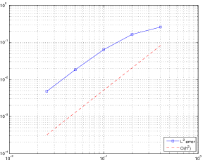
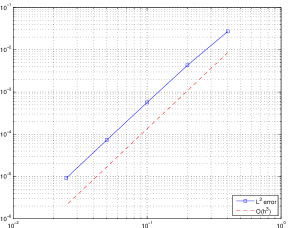
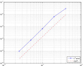
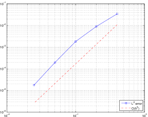
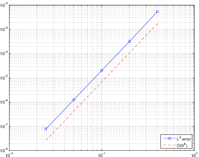
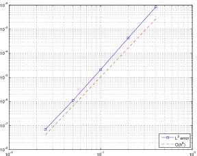
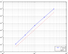
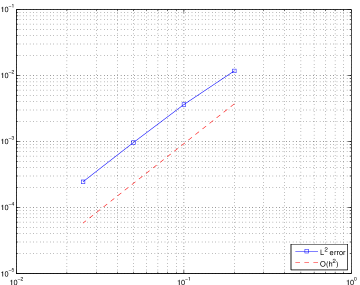
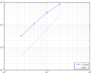
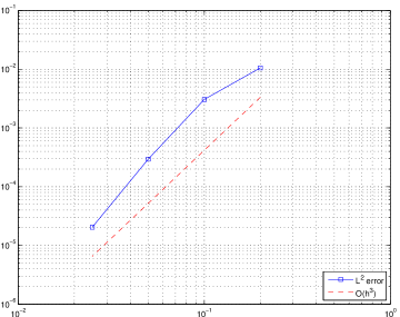
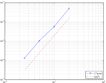
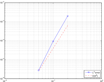
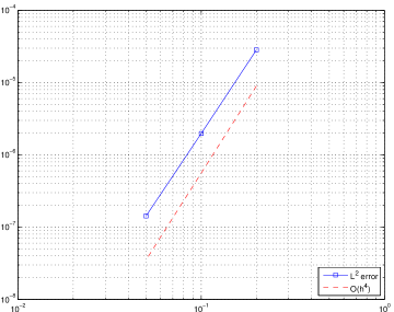
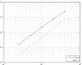
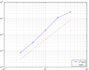
Fig. 1 shows the L2superscript𝐿2L^{2} convergence results for uhsubscript𝑢u_{h} for LS-weak. Actually, that optimal convergence rates are obtained, which is better than the theoretical result in Theorem 2.3. The convergence rates of LS-strong is the same.
Refer to caption
Refer to caption
Refer to caption
Refer to caption
Refer to caption
Refer to caption
Refer to caption
Refer to caption
Refer to caption
Figure 1. Convergence test for a smooth solution. Left–Right: ε=1𝜀1\varepsilon=1, 103superscript10310^{-3} and 109superscript10910^{-9}. Top–Bottom: P1𝑃1P1P3𝑃3P3.

6.2. A rotating flow test

We take ϵ=106italic-ϵsuperscript106\epsilon=10^{-6}, 𝜷=[y1/2,1/2x]T𝜷superscript𝑦1212𝑥𝑇\boldsymbol{\beta}=[y-1/2,1/2-x]^{T}, and f=0𝑓0f=0. The solution u𝑢u is prescribed along the slip 1/2×[0,1/2]120121/2\times[0,1/2] by

u(1/2,y)=sin2(2πy)y[0,1/2].formulae-sequence𝑢12𝑦superscript22𝜋𝑦𝑦012u(1/2,y)=\sin^{2}(2\pi\,y)\qquad y\in[0,1/2].

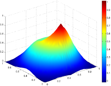
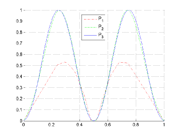
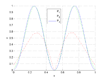
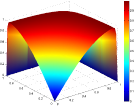
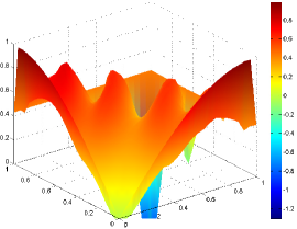
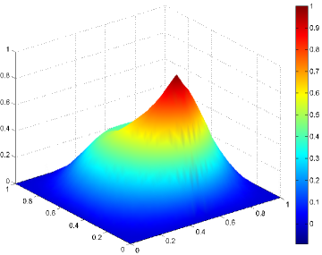
We refer to [42] for a detailed description of this test. In Fig. 2, we plot uhsubscript𝑢u_{h} obtained from the two first order least squares methods for various polynomial degrees in an unstructured triangular grid of 592 elements. Notice that both methods produce similar results, and there is a significant improvement of the result from P𝑃P1 to P𝑃P2. In addition, the use of higher polynomial degree leads to smoother approximations, see Fig. 3 for a comparison between different polynomial degrees.
Refer to caption
Refer to caption
Refer to caption
Refer to caption
Refer to caption
Refer to caption
Figure 2. 3D plot of uhsubscript𝑢u_{h} for rotating flow test with ϵ=106italic-ϵsuperscript106\epsilon=10^{-6} in 592 elements. Left–Right: LS–strong, LS–weak. Top–Bottom: P1𝑃1P1P3𝑃3P3.
Refer to caption
Refer to caption
Figure 3. Profile of the approximate solution at y=1/2𝑦12y=1/2 when ε=109𝜀superscript109\varepsilon=10^{-9}. Left–Right: LS–strong, LS–weak.

6.3. An interior layer test

We take 𝜷=[1/2,3/2]T𝜷superscript1232𝑇\boldsymbol{\beta}=[1/2,\sqrt{3}/2]^{T}, f=0𝑓0f=0, and Dirichlet boundary conditions as follows:

u={1on {y=0,0x1},1on {x=0,0y1/5},0elsewhere.\displaystyle u=\left\{\begin{tabular}[]{l l}$1$&{ on }$\{y=0,0\leq x\leq 1\}$,\\ $1$&{ on }$\{x=0,0\leq y\leq 1/5\}$,\\ $0$&{ elsewhere.}\end{tabular}\right.

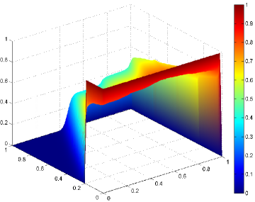
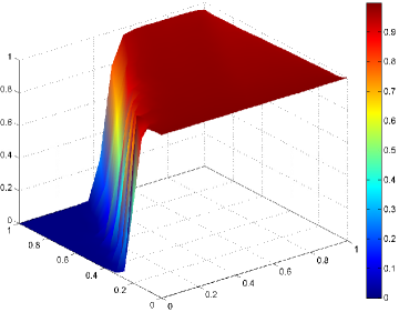
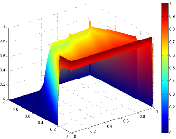
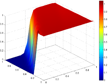
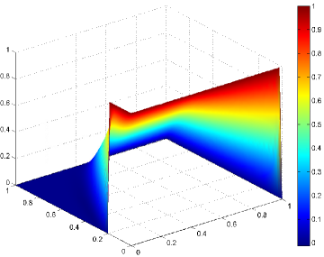
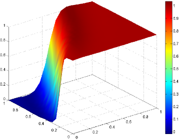
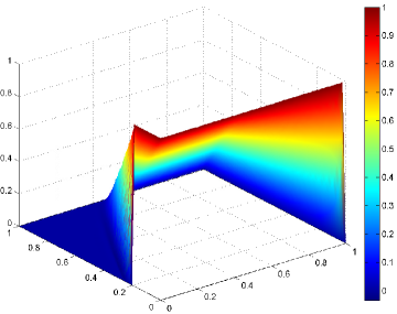
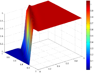
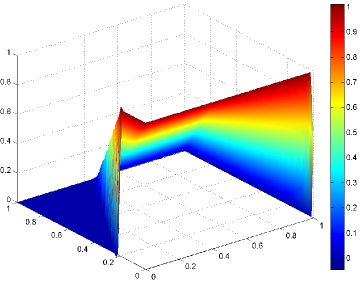
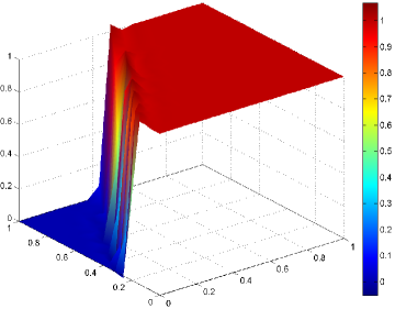
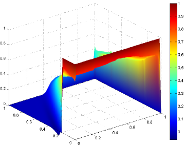
In Fig. 4 and Fig. 5, we plot uhsubscript𝑢u_{h} obtained from the two first order least squares methods for ϵ=103italic-ϵsuperscript103\epsilon=10^{-3} and ϵ=109italic-ϵsuperscript109\epsilon=10^{-9}, respectively. Though the exact solution of this example is not available, it is easy to see that the result produced by LS-weak is much more accurate. Fig. 4 and Fig. 5 imply that uhsubscript𝑢u_{h} produced by LS-strong in 11264 element is almost totally collapsed, while LS-weak can have much better approximation in a much coarser mesh with 704 elements.

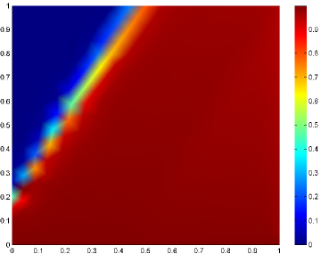
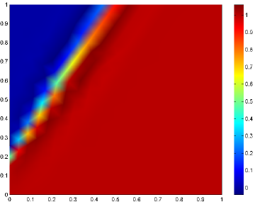
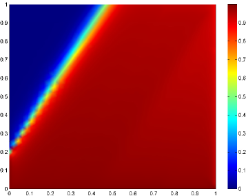
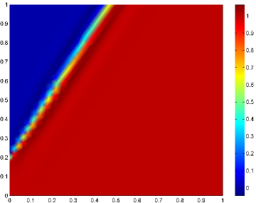
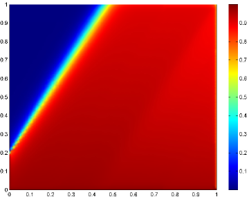
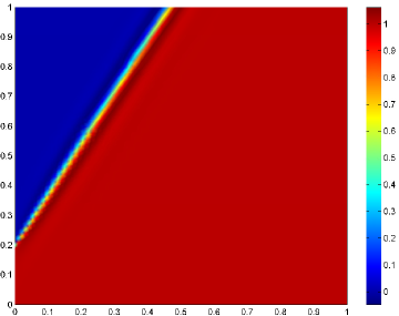
In order to illustrate the behavior of LS-weak in capturing the interior layers, in Fig. 6, we plot the contour plot of LS-weak using P𝑃P2 for three consecutive meshes. We observe finer mesh leads to sharper layer width.
Refer to caption
Refer to caption
Refer to caption
Refer to caption
Refer to caption
Refer to caption
Figure 4. 3D plot of uhsubscript𝑢u_{h} for interior layer test with ϵ=103italic-ϵsuperscript103\epsilon=10^{-3}. Left–Right: LS–strong in 11264 elements, LS-weak in 704 elements. Top–Bottom: P1𝑃1P1P3𝑃3P3.
Refer to caption
Refer to caption
Refer to caption
Refer to caption
Refer to caption
Refer to caption
Figure 5. 3D plot of uhsubscript𝑢u_{h} for interior layer test with ϵ=109italic-ϵsuperscript109\epsilon=10^{-9}. Left–Right: LS–strong in 11264 elements, LS-weak in 704 elements. Top–Bottom: P1𝑃1P1P3𝑃3P3.
Refer to caption
Refer to caption
Refer to caption
Refer to caption
Refer to caption
Refer to caption
Figure 6. Contour plot of uhsubscript𝑢u_{h} for interior layer test using LS–weak P𝑃P2. Left: ϵ=103italic-ϵsuperscript103\epsilon=10^{-3}; Right: ϵ=109italic-ϵsuperscript109\epsilon=10^{-9}. Top: 704 elements; Middle: 2816 element; Bottom: 11264 elements.

6.4. A boundary layer test

Finally, we take 𝜷=[1,1]T𝜷superscript11𝑇\boldsymbol{\beta}=[1,1]^{T}, and choose the source term f𝑓f such that the exact solution

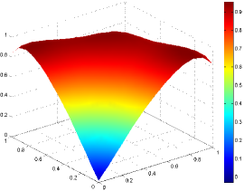
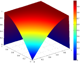
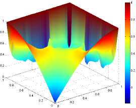
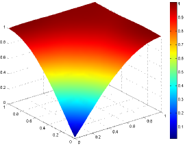
u(x,y)=sinπx2+sinπy2(1sinπx2)+e1/ϵe(1x)(1y)/ϵ1e1/ϵ.𝑢𝑥𝑦𝜋𝑥2𝜋𝑦21𝜋𝑥2superscript𝑒1italic-ϵsuperscript𝑒1𝑥1𝑦italic-ϵ1superscript𝑒1italic-ϵu(x,y)=\sin\frac{\pi\,x}{2}+\sin\frac{\pi\,y}{2}\left(1-\sin\frac{\pi\,x}{2}\right)+\frac{e^{-1/\epsilon}-e^{-(1-x)(1-y)/\epsilon}}{1-e^{-1/\epsilon}}.

The solution develops boundary layers along the boundaries x=1𝑥1x=1 and y=1𝑦1y=1 for small ϵitalic-ϵ\epsilon (see Fig. 7). Let us emphasize that our exact solution is different from that of [1] in order to have a better observation of the local convergence results for higher degree approximations. In Fig. 7, we plot the exact solution and computational results for ϵ=102,106,109italic-ϵsuperscript102superscript106superscript109\epsilon=10^{-2},10^{-6},10^{-9}. We notice that the numerical solutions produced by LS-strong are totally polluted by boundary layers, while LS-weak can produce numerical solutions very close to the exact ones except in area very close to boundary layers.

In Fig. 8, we show the convergence of uhsubscript𝑢u_{h} produced by LS–weak in L2superscript𝐿2L^{2}–norm for ϵ=102,109italic-ϵsuperscript102superscript109\epsilon=10^{-2},10^{-9} in the subdomain Ω~=[0,0.9]×[0,0.9]Ω~Ω00.900.9Ω\widetilde{\Omega}=[0,0.9]\times[0,0.9]\subset\Omega to exclude the unresolved boundary layer. We notice that the accuracy of uhsubscript𝑢u_{h} in Ω~~Ω\tilde{\Omega} is not affected by boundary layers.

Refer to caption
Refer to caption
Refer to caption
Refer to caption
Refer to caption
Refer to caption
Refer to caption
Refer to caption
Refer to caption
Figure 7. 3D plot of u𝑢u for the boundary layer test. Top: ϵ=102italic-ϵsuperscript102\epsilon=10^{-2}; Middle: ϵ=106italic-ϵsuperscript106\epsilon=10^{-6}; Bottom: ϵ=109italic-ϵsuperscript109\epsilon=10^{-9}. Left: exact solution; Middle: LS–strong in 1664 elements using P2; Right: LS–weak in 416 elements using P1.
Refer to caption
Refer to caption
Refer to caption
Refer to caption
Refer to caption
Refer to caption
Figure 8. Convergence history of uhsubscript𝑢u_{h} produced by LS-weak at the subdoamin (0,0.9)×(0,0.9)00.900.9(0,0.9)\times(0,0.9) away from the boundary layer. Left–right: ϵ=102italic-ϵsuperscript102\epsilon=10^{-2},ϵ=109italic-ϵsuperscript109\epsilon=10^{-9}. Top–Bottom: P1𝑃1P1P3𝑃3P3.

7. Extension to transportation reaction problems

We present first order least squares method for the transportation reaction problems

𝜷u+cu=𝜷𝑢𝑐𝑢absent\displaystyle\boldsymbol{\beta}\cdot\nabla u+cu= f in Ω,𝑓 in Ω,\displaystyle\;f\quad\text{ in $\Omega$, } (7.1a)
u=𝑢absent\displaystyle u= g on Γ={xΩ:𝜷𝒏(x)<0}.𝑔 on Γ={xΩ:𝜷𝒏(x)<0}.\displaystyle\;g\quad\text{ on $\Gamma^{-}=\{x\in\partial\Omega:\boldsymbol{\beta}\cdot\boldsymbol{n}(x)<0\}$. } (7.1b)

The first order least squares method is to find uhWhsubscript𝑢subscript𝑊u_{h}\in W_{h} satisfying

(𝜷uh+cuh,𝜷w+cw)Ωsubscript𝜷subscript𝑢𝑐subscript𝑢𝜷𝑤𝑐𝑤Ω\displaystyle\left(\boldsymbol{\beta}\cdot\nabla u_{h}+cu_{h},\boldsymbol{\beta}\cdot\nabla w+cw\right)_{\Omega} (7.2)
+ΣFhhF1max(𝜷𝒏(x),0)uh,wFsubscriptΣ𝐹superscriptsubscriptsuperscriptsubscript𝐹1subscript𝜷𝒏𝑥0subscript𝑢𝑤𝐹\displaystyle\quad+\Sigma_{F\in\mathcal{E}_{h}^{\partial}}h_{F}^{-1}\langle\max(-\boldsymbol{\beta}\cdot\boldsymbol{n}(x),0)u_{h},w\rangle_{F}
=\displaystyle= (f,𝜷w+cw)Ωsubscript𝑓𝜷𝑤𝑐𝑤Ω\displaystyle(f,\boldsymbol{\beta}\cdot\nabla w+cw)_{\Omega}
+ΣFhhF1max(𝜷𝒏(x),0)g,wF,w𝒰h.subscriptΣ𝐹superscriptsubscriptsuperscriptsubscript𝐹1subscript𝜷𝒏𝑥0𝑔𝑤𝐹for-all𝑤subscript𝒰\displaystyle\quad+\Sigma_{F\in\mathcal{E}_{h}^{\partial}}h_{F}^{-1}\langle\max(-\boldsymbol{\beta}\cdot\boldsymbol{n}(x),0)g,w\rangle_{F},\quad\forall w\in\mathcal{U}_{h}.

Here, 𝒰h={w|KH1(Ω):wPk+1(K),K𝒯h}\mathcal{U}_{h}=\{w|_{K}\in H^{1}(\Omega):w\in P_{k+1}(K),\quad\forall K\in\mathcal{T}_{h}\}.

Obviously, (7.2) is a special case of first order least squares method (2.4) when the diffusion coefficient is zero. By using similar argument in section 4.1, we have the following Theorem 7.1.

Theorem 7.1.

Let u𝑢u be the solution of transport reaction equation (7.1) and uhsubscript𝑢u_{h} the numerical solution of first order least squares method (7.2).

uuhL2(Ω)+𝜷(uuh)L2(Ω)Chk+1uHk+2(Ω).subscriptnorm𝑢subscript𝑢superscript𝐿2Ωsubscriptnorm𝜷𝑢subscript𝑢superscript𝐿2Ω𝐶superscript𝑘1subscriptnorm𝑢superscript𝐻𝑘2Ω\displaystyle\|u-u_{h}\|_{L^{2}(\Omega)}+\|\boldsymbol{\beta}\cdot\nabla(u-u_{h})\|_{L^{2}(\Omega)}\leq Ch^{k+1}\|u\|_{H^{k+2}(\Omega)}. (7.3)
Remark 7.2.

The first order least squares method (7.2) is the same as the method in [4], except the way of imposing boundary condition. In [4], the term c12𝜷𝑐12𝜷c-\frac{1}{2}\nabla\cdot\boldsymbol{\beta} is required to be uniformly bounded from below by a positive constant. We get rid of this restriction.

Acknowledgements. The work of Huangxin Chen was supported by the NSF of China (No. 11201394) and the NSF of Fujian Province (No. 2013J05016). The work of Jingzhi Li was supported by the NSF of China (No. 11201453 and 91130022). The work of Weifeng Qiu was supported by City University of Hong Kong under start-up grant (No. 7200324) and by the GRF of Hong Kong (Grant No. 9041980).

References

  • [1] B. Ayuso and D. Marini, Discontinuous Galerkin Methods for Advection-Diffusion-Reaction Problems, SIAM J. Numer. Anal., 47(2) (2009), 1391–1420.
  • [2] Y. Bazilevs and T.J.R. Hughes, Weak imposition of Dirichlet boundary conditions in fluid mechanics, Compt. & Fluids, 36(1) (2007), 12–26.
  • [3] D.  Broersen and R. Stevenson, A Petrov-Galerkin discretization with optimal test space of a mild-weak formulation of convection-diffusion equations in mixed form, IMA J. Numer. Anal., (2014), Accepted.
  • [4] P.B. Bochev and J. Choi, Improved least-squares error estimates for scalar hyperbolic problems, Computational Methods in Applied Mathematics, 1(1) (2001), 1–8.
  • [5] P.B. Bochev and M.D. Gunzburger, Analysis of least-squares finite element methods for the Stokes equations, Math. Comp., 63 (1994), 479–506.
  • [6] P.B. Bochev and M.D. Gunzburger, Finite element methods of least-squares type, SIAM Rev., 40 (1998), 789–837.
  • [7] P.B. Bochev and M.D. Gunzburger, Least-squares finite element methods, Appl. Math. Sci., 166, Springer, New York, 2009.
  • [8] F. Brezzi, T.J.R. Hughes, L.D. Marini, A. Russo and E. Süli, A Priori Error Analysis of Residual-free Bubbles for Advection-Diffusion Problems, SIAM J. Numer. Anal., 36(6) (1999), 1933–1948.
  • [9] F. Brezzi, L.D. Marini, and E. Süli, Residual-free bubbles for advection-diffusion problems: the general error analysis, Numer. Math., 85 (2000), 31–47.
  • [10] A. N. Brooks and T.J.R. Hughes, Streamline upwind/Petrov-Galerkin formulations for convection dominated flows with particular emphasis on the incompressible Navier-Stokes equations, Comput. Methods Appl. Mech. Engrg., 32 (1982), 199–259.
  • [11] T. Bui-Thanh, L. Demkowicz and O. Ghattas, A Unified Discontinuous Petrov–Galerkin Method and Its Analysis for Friedrichs’ Systems, SIAM J. Numer. Anal., 51(4) (2013), 1933–1958.
  • [12] Erik Burman, A Unified Analysis for Conforming and Nonconforming Stabilized Finite Element Methods Using Interior Penalty, SIAM J. Numer. Anal., 43(5) (2005), 2012–2033.
  • [13] Erik Burman and Alexandre Ern, Stabilized Galerkin Approximation of Convection-Diffusion-Reaction equations: Discrete Maximum Principle and Convergence, Math. Comp., 74 (2005), 1637–1652.
  • [14] Z. Cai, Least squares for the perturbed Stokes equations and the Reissner-Mindlin plate, SIAM J. Numer. Anal., 38(5) (2000), 1561–1581.
  • [15] Z. Cai, R. Lazarov, T.A. Manteuffel and S.F. McCormick, First-order system least squares for second-order partial differential equations: Part I, SIAM J. Numer. Anal., 31 (1994), 1785–1799.
  • [16] Z. Cai, T.A. Manteuffel and S.F. McCormick, First-order system least squares for second-order partial differential equations: Part II, SIAM J. Numer. Anal., 34 (1997), 425–454.
  • [17] Z. Cai, B. Lee and P. Wang, Least-squares methods for incompressible Newtonian fluid flow: linear stationary problems, SIAM J. Numer. Anal., 42(2) (2004), 843–859.
  • [18] Z. Cai and G. Starke, Least-squares methods for linear elasticity, SIAM J. Numer. Anal., 42(2) (2004), 826–842.
  • [19] Z. Cai and C. R.  Westphal, A weighted H(div) least-squares method for second-order elliptic problems, SIAM J. Numer. Anal., 46(3) (2008), 1640–1651.
  • [20] J. Chan, N. Heuer, T. Bui-Thanh and L. Demkowicz, A robust DPG method for convection-dominated diffusion problems II: Adjoint boundary conditions and mesh-dependent test norms, Computers & Mathematics with Applications, 67(4) (2014), 771–795.
  • [21] C.L. Chang and B.N. Jiang, An error analysis of least-squares finite element method of velocity-pressure-vorticity formulation for Stokes problem, Computer Methods in Applied Mechanics and Engineering, 84 (1990), 247–255.
  • [22] C.L. Chang, S.Y. Yang and C.H. Hsu, A least-squares finite element method for incompressible flow in stress-velocity-pressure version, Computer Methods in Applied Mechanics and Engineering, 128 (1995), 1–9.
  • [23] C.L. Chang and S.Y. Yang, Analysis of the L2superscript𝐿2L^{2} least-squares finite element method for the velocity-vorticity-pressure Stokes equations with velocity boundary conditions, Appl. Math. Comp., 130 (2002), 121–144.
  • [24] A. Cohen, W. Dahmen and G. Welper, Adaptivity and variational stabilization for convection-diffusion equations, ESAIM Math. Model. Numer. Anal., 46 (2012), 1247–1273.
  • [25] W. Dahmen, C. Huang, C. Schwab and G. Welper, Adaptive Petrov-Galerkin methods for first order transport equations, SIAM J. Numer. Anal., 50 (2012), 2420–2445.
  • [26] J.M. Deang and M.D. Gunzburger, Issues related to least-squares finite element methods for the Stokes equations, SIAM J. Sci. Comput., 20 (1998), 878–906.
  • [27] L. Demkowicz and J. Gopalakrishnan, A class of discontinuous Petrov-Galerkin methods. Part I: The transport equation, Computer Methods in Applied Mechanics and Engineering, 199 (2010), 1558–1572.
  • [28]  , A class of discontinuous Petrov-Galerkin methods. Part II: Optimal test functions, Numerical Methods for Partial Differential Equations, 27 (2011), 70–105.
  • [29]  , Analysis of the DPG method for the Poisson equation, SIAM J. Numer. Anal., 49(5) (2011), 1788–1809.
  • [30] L. Demkowicz, J. Gopalakrishnan, and A. Niemi, A class of discontinuous Petrov-Galerkin methods. Part III: Adaptivity, Applied Numerical Mathematics, 62 (2012), 396–427.
  • [31] L. Demkowicz and N. Heuer, Robust DPG Method for Convection-Dominated Diffusion Problems, SIAM J. Numer. Anal., 51(5) (2013), 2514–2537.
  • [32] D. Di Pietro, A. Ern and J.L. Guermond, Discontinuous Galerkin methods for anisotropic semi-definite diffusion with advection, SIAM J. Num. Anal., 46(2) (2008), 805–831.
  • [33] A. Ern, F. Stephansen and P. Zunino, A Discontinuous Galerkin method with weighted averages for advection–diffusion equations with locally small and anisotropic diffusivity, IMA J. Num. Anal., 29(2) (2009), 235–256.
  • [34] A. Ern and J.L. Guermond, Discontinuous Galerkin Methods for Friedrichs’ systems. I. General theory, SIAM J. Num. Anal., 44(2) (2006), 753–778.
  • [35]  , Discontinuous Galerkin Methods for Friedrichs’ systems. II. Second-Order PDES, SIAM J. Num. Anal., 44(6) (2006), 2363–238.
  • [36]  , Discontinuous Galerkin Methods for Friedrichs’ systems, Part III. Multifield Theories with partial coercivity, SIAM J. Num. Anal., 46(2) (2008), 776–804.
  • [37] J.M. Fiard, T.A. Manteuffel and S.F. McCormick, First-order system least squares (FOSLS) for convection-diffusion problems: Numerical results, SIAM J. Sci. Comput., 19 (1998), 1958–1979.
  • [38] H. Goering, A. Felgenhauer, G. Lube, H.-G. Roos, and L. Tobiska, Singularly perturbed differential equations, Akademie-Verlag, Berlin 1983.
  • [39] J. Gopalakrishnan and W. Qiu, An analysis of the practical DPG method, Math. Comp., 83 (2014), 537–552 .
  • [40] P. Houston, C. Schwab and E. Süli, Discontinuous hp-finite element methods for advection-diffusion-reaction problems, SIAM J. Num. Anal., 39(6) (2002), 2133–2163.
  • [41] P.W. Hsieh and S.Y. Yang, A novel least-squares finite element method enriched with residual-free bubbles for solving convection-dominated problems, SIAM J. Sci. Comput., 32(4) (2010), 2047–2073.
  • [42] T.J.R. Hughes, G. Scovazzi, P. Bochev and A. Buffa, A multiscale discontinuous Galerkin method with the computational structure of a continuous Galerkin method, Comput. Methods Appl. Mech. Engrg., 195(19-22) (2006), 2761–2787.
  • [43] B.N. Jiang, The Least-squares Finite Element Method, Springer-Verlag, Berlin, 1998.
  • [44] C. Johnson and J. Pitkäranta, An analysis of the discontinuous Galerkin method for a scalar hyperbolic equation, Math. Comp., 46 (1986), 1–26.
  • [45] R. Lazarov, L. Tobiska, and P. S. Vassilevski, Streamline diffusion least-squares mixed finite element methods for convection-diffusion problems, East-West J. Numer. Math., 5 (1997), 249–264.
  • [46] B. Lee, First-order system least-squares for elliptic problems with Robin boundary conditions, SIAM J. Numer. Anal., 37 (1999), 70–104.
  • [47] J. Nitsche, Über ein Variationsprinzip zur Lösung von Dirichlet-Problemen bei Verwendung von Teilräumen, die keinen Randbedingungen unterworfen sind., Abh. Math. Sem. Univ. Hamburg, 36 (1971), 9–15.
  • [48] A.I. Pehlivanov, G.F. Carey, and R. Lazarov, Least-squares mixed finite elements for second-order elliptic problems, SIAM J. Numer. Anal., 31 (1994), 1368–1377.
  • [49] W. Reed and T. Hill, Triangular mesh methods for the neutron transport equation, Technical Report LA- UR-73-479, Los Alamos Scientific Laboratory, (1973).
  • [50] H.-G. Roos, M. Stynes, and L. Tobiska, Robust numerical methods for singularly perturbed differential equations, volume 24 of Springer Series in Computational Mathematics. Springer-Verlag, Berlin, 2008. Convection-diffusion and flow problems. Second edition.
  • [51] F. Schieweck, On the role of boundary conditions for CIP stabilization of higher order finite elements, Electron. Trans. Numer. Anal., 32 (2008), 1–16.
  • [52] M. Stynes, Steady­ state convection­ diffusion problems, Acta Numer., 14 (2005), 445–508.