Next-to-leading order QCD corrections to five jet production at the LHC
Abstract
We present theoretical predictions for five jet production in proton-proton collisions at next-to-leading order accuracy in QCD. Inclusive as well as differential observables are studied for collision energies of 7 and 8 TeV. In general the next-to-leading order corrections stabilize the theoretical predictions with respect to scale variations. In case of the inclusive jet cross sections, we compare with experimental data where possible and find reasonable agreement. We observe that the four-to-three and five-to-four jet ratios show better perturbative convergence than the known three-to-two ratio and are promising candidates for future measurements. Furthermore, we present a detailed analysis of uncertainties related to parton distribution functions. The full colour virtual matrix elements used in the computation were obtained with the NJet package Badger et al. (2013a), a publicly available library for the evaluation of one-loop amplitudes in massless QCD.
pacs:
12.38.Bx, 14.65.HaI Introduction
The wealth of data recorded at the LHC experiments in run 1 presents an excellent opportunity to test quantum chromo-dynamics (QCD) in a new energy regime. Furthermore, multi-jet production at large transverse momentum can provide useful information to constrain the parton distribution functions. Where precise theoretical results are available, the data can also be used to determine the strong coupling constant . In that context large multiplicities may turn out to be particularly useful, in analogy to what has been observed in electron-positron annihilation. Pure QCD reactions with multiple jet production can also give large backgrounds to various new physics searches therefore precision predictions are required.
Next-to-leading order (NLO) predictions at fixed order in for di-jet production have been known for more than 20 years Giele et al. (1993). Three-jet production represents a considerable increase in computational complexity and a full computation was completed in 2002 Nagy (2002), and implemented in the public code NLOJET++, though pure gluonic contributions were known previously Kilgore and Giele (1997). Breakthroughs in virtual amplitude computations have recently enabled predictions of four-jet production Bern et al. (2012); Badger et al. (2013b), with results generally in good agreement with the experimental data Aad et al. (2011). Di-jet production is known to suffer from large corrections from soft gluon radiation which requires resummation beyond fixed order perturbation theory. Theoretical predictions at NLO including the parton shower (NLO+PS) allow to account for these effects and obtain a better description of the available data Alioli et al. (2011); Hoeche and Schonherr (2012). The CMS collaboration has recently completed a measurement of from the inclusive 3-jet to inclusive 2-jet ratio. The measurement illustrates well the LHC potential for precision measurements. With NNLO QCD corrections to di-jet production just around the corner Ridder et al. (2013), theoretical uncertainties look to be under good control and enable future QCD predictions to move beyond the ‘industry standard’ LO+PS/ME+PS accuracy.
By now there has been a great success of the program to automate NLO computations. Processes with four or five final state particles, previously thought to be impossible, are now available in public codes Badger et al. (2011); Hirschi et al. (2011); Bevilacqua et al. (2011); Cullen et al. (2012); Badger et al. (2013a). New methods and algorithms Cascioli et al. (2012); Becker et al. (2012); Actis et al. (2013) have been pushing the boundaries of perturbative QCD computations and increasing the range of phenomenological applications (recent examples can be found in Bevilacqua and Worek (2012); Bern et al. (2013); Cullen et al. (2013); van Deurzen et al. (2013); Gehrmann et al. (2013), see also Alcaraz Maestre et al. (2012) for a more complete overview). Powerful on-shell unitarity methods have been established for many years Bern et al. (1994, 1995) yet continue to demonstrate the ability to simplify calculations of extremely high multiplicity amplitudes inaccessible with alternative tools. Recent state-of-the-art computations include the NLO QCD corrections to jets Bern et al. (2013) by the BlackHat collaboration. In this paper we present the first computation for the production of five hard jets at NLO in QCD.
The article is organized as follows: we first give an overview of the computational framework for the various partonic sub-channels in Section II. Section III contains our results for the NLO QCD corrections to jets. We describe the numerical setup and interface with the Sherpa Monte-Carlo event generator Gleisberg et al. (2009) in Section III.1 along with kinematic cuts. Results for total cross sections and jet ratios are compared to the available data in Section III.2. We present differential distributions in the jet transverse momenta and rapidity and perform a detailed comparison of different PDF fits. We finally present our conclusions and outlook for the future. Two appendices containing a complete set of distributions and numerical values used in the plotted histograms are included to ease future comparisons.
II Outline of the calculation
The calculation is done in QCD with five massless quark flavours including the bottom-quark in the initial state. We expect the neglected contributions from top quark loops to be much smaller than the estimated theoretical uncertainty. The processes contributing to five-jet production may be derived from the following four basic channels via crossing symmetry
where , and denote generic quarks of different flavour. Amplitudes with like-flavour quark pairs can always be obtained from the amplitudes for different flavours by an appropriate (anti) symmetrization. The -jet differential cross section expanded in the coupling reads
| (1) |
where and . In the QCD improved parton model, the leading order differential cross section is given by
| (2) |
are the momenta of the two incoming hadrons which we assume to be massless. The total incoming momentum of the initial state partons leads to a partonic centre-of-mass energy squared with being the hadronic centre-of-mass energy squared. The parton distribution functions describe, roughly speaking, the probability to find a parton inside a hadron with a momentum fraction between and . Note that the parton distribution functions depend besides also on the unphysical factorization scale . The partonic differential cross section describes the reaction in Born approximation using the leading order matrix elements and a suitable jet algorithm :
| (3) |
are the four momenta of the outgoing partons obeying . The jet algorithm is a function depending solely on the final state parton momenta and on parameters defining the geometric extensions of the jet. Its value is equal to one if the final state momentum configuration corresponds to a valid -jet event and zero otherwise. The Born matrix elements have been evaluated with Comix Gleisberg and Hoeche (2008) within the Sherpa framework. The Sherpa Monte Carlo event generator Gleisberg and Krauss (2008) has also been used to perform the numerical phase space integration.
At NLO accuracy both the virtual corrections (one-loop contribution interfered with the Born amplitude) and the real corrections (tree-level amplitudes with one additional parton in the final state) contribute to the -jet cross section. Both and contain separately collinear and soft divergences. Only after combining the two contributions and factorizing the initial state singularities into renormalized parton distributions one obtains a finite result. In order to perform the cancellation of the divergences numerically we apply the Catani-Seymour subtraction method Catani and Seymour (1996). The idea is to add and subtract local counter-terms with -parton kinematics which, on the one hand, mimic point-wise the singularity structure of the real corrections and which, on the other hand, are chosen such that the singularity due to the additional parton emission can be calculated analytically via separate integration of the one-particle phase-space. Since the latter cancel by construction the divergences from the virtual corrections, only finite quantities remain making the numerical integration with a Monte Carlo program feasible. Schematically, we may write the total cross section as
| (4) |
is due to the factorization of initial state singularities. The NLO corrections can then be written in terms of three finite contributions:
| (5) |
denotes the finite part of the virtual corrections, the finite part of the integrated subtraction terms together with the contribution from the factorization and the real corrections combined with the subtraction terms. For the computation of and we use Sherpa which provides a numerical implementation of the Catani-Seymour subtraction scheme. The required tree-level amplitudes are, as in the LO case, computed with Comix as part of the Sherpa framework.
The necessary one-loop matrix elements for the virtual corrections are
evaluated with the publicly available NJet 111To download NJet visit the project home page
at
https://bitbucket.org/njet/njet/. package Badger et al. (2013a). NJet uses an on-shell
generalized unitarity framework Britto et al. (2005); Ellis et al. (2008); Forde (2007); Berger et al. (2008) to
compute multi-parton one-loop primitive amplitudes from tree-level building blocks. An accurate
numerical implementation is achieved using the integrand reduction procedure of OPP
Ossola et al. (2007). The algorithm is based on the NGluon library Badger et al. (2011) following
the description of -dimensional generalized unitarity presented in Refs.
Giele et al. (2008); Badger (2009) and using Berends-Giele recursion Berends and Giele (1988) for
efficient numerical evaluation of tree-level amplitudes. For a more detailed description of the employed
methods and the usage of the program, we refer to Refs. Badger et al. (2011, 2013a). The
scalar loop integrals are obtained via the QCDLoop/FF package
van Oldenborgh (1991); Ellis and Zanderighi (2008). We note that NJet is so far the only publicly available
tool that is able to compute all one-loop seven-point matrix-elements that contribute to five-jet
production in hadronic collisions. For reference numerical evaluations of the one-loop matrix
elements at a single phase-space point have been presented previously Badger et al. (2013a).
III Results for 5-Jet production at the LHC at 7 and 8 TeV
III.1 Numerical setup
As mentioned earlier we use the Sherpa Monte-Carlo event generator Gleisberg et al. (2009) to handle phase-space integration and generation of tree-level and Catani-Seymour dipole subtraction terms using the colour dressed formalism implemented in Comix Gleisberg and Hoeche (2008); Gleisberg and Krauss (2008). The virtual matrix elements are interfaced using the Binoth Les Houches Accord Binoth et al. (2010); Alioli et al. (2013).
To combine partons into jets we use the anti-kt jet clustering algorithm as implemented in FastJet Cacciari et al. (2012, 2008). Furthermore asymmetric cuts on the jets ordered in transverse momenta, , are applied to match the ATLAS multi-jet measurements Aad et al. (2011):
| (6) |
The PDFs are accessed through the LHAPDF interface Whalley et al. (2005) with all central values using NNPDF2.1 Ball et al. (2012) for LO () and NNPDF2.3 Ball et al. (2013) for NLO () if not mentioned otherwise.
Generated events are stored in Root Ntuple format Andersen et al. (2010) which allows for flexible analysis. Renormalization and factorization dependence can be re-weighted at the analysis level as well as the choice of PDF set. Since the event generation of high multiplicity processes at NLO is computationally intensive analysis of PDF uncertainties and scale choices would be prohibitive without this technique.
III.2 Numerical results
In this section we present the numerical results for total cross sections and selected222The complete set of results presented in this section together with additional distributions for 7 and 8 TeV can be obtained from https://bitbucket.org/njet/njet/wiki/Results/Physics. distributions at centre-of-mass energies of 7 and 8 TeV. Within the setup described in the previous section we have chosen the renormalization and factorization scales to be equal and use a dynamical scale based on the total transverse momentum of the final state partons:
| (7) |
We then obtain the 5-jet cross section at 7 TeV,
where numerical integration errors are quoted in parentheses. We show the values of the cross section at three values of the renormalization scale, where . We observe significant reduction in the residual scale dependence when including NLO corrections. Within the chosen scale band, the LO predictions lie within a range of nb while at NLO the range is nb. The analagous results at 8 TeV are shown below.
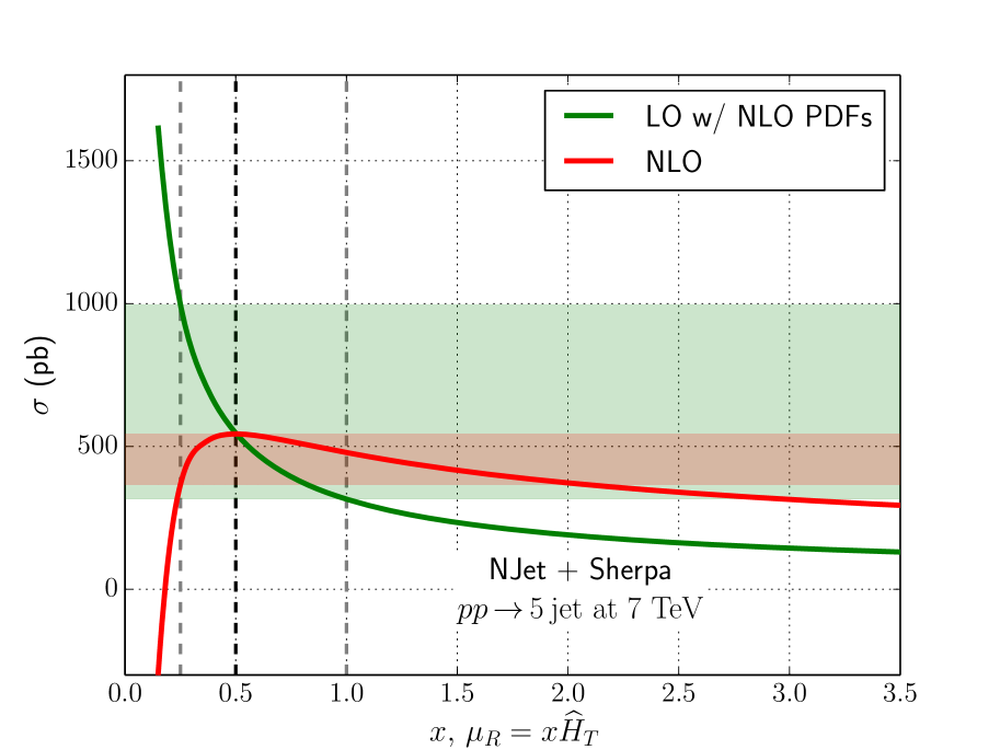
In Fig. 1 the scale dependence of the leading order and next-to-leading order cross section is illustrated. The dashed black line indicates . The horizontal bands show the variation of the cross section for a scale variation between and . The uncertainty due to scale variation is roughly reduced by a factor of one third. Furthermore we see that around the NLO cross section is flat indicating that is a reasonable choice for the central scale. This is further supported by the fact that for the NLO corrections are very small. It is also interesting to observe that the two bands, LO and NLO, nicely overlap. Note however that we have used the NLO setup in the leading order calculation. In particular the NLO PDFs with the corresponding are employed.
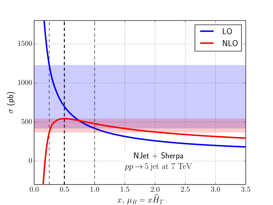
In Fig. 2 we show the scale dependence using in the leading order prediction LO PDFs with the respective . Compared to Fig. 1 we observe in Fig. 2 a much larger difference between the LO and NLO prediction. To some extend the difference is due to the change in . Similar to what has been found in Ref. Badger et al. (2013b) we conclude that using the NLO PDFs in the LO predictions gives a better approximation to the full result compared to using LO PDFs.
Although not a physical observable it is interesting to ask how the different partonic channels contribute to the inclusive 5-jet rate. Ignoring different quark flavours we distinguish nine partonic channels in LO:
where may be any quark or anti-quark with exception of the top-quark i.e. . In Tab. 1 the individual contribution of each channel is presented.
| . | ||
| . | ||
| . | ||
| . | ||
| . | ||
| . | ||
| . | ||
| . | ||
| . |
The most important contribution is provided by the initial state. Almost 50% of the cross section can be attributed to this channel. This is a consequence of the large parton luminosity in combination with the sizeable cross sections. Among the initiated reactions the channel is with about 40% of the cross section the most important process. Replacing the quark line in this process by a gluon will still lead to large partonic cross sections. However the parton flux is reduced compared to the initial state. As a consequence the purely gluonic reaction leads to a slightly smaller contribution and is responsible for about 25% of the cross section. The composition of the cross section may provide useful information when jet rates are used to constrain the PDFs. Since the luminosity functions
| (8) |
depend on the partonic centre-of-mass energy, the composition may be different for different kinematical configurations. We come back to this point when we discuss differential distributions.
In Tab. 2 we show for completeness the cross sections for two, three and four-jet production as calculated with NJet using the same setup as in the five jet case.
The real corrections to five-jet production allow us to calculate also the cross section for six jet production, however only in leading order QCD. The result is given by
where the NNPDF2.3 NLO PDF set with has been used. The jet rates have been measured recently by ATLAS using the 7 TeV data set Aad et al. (2011).
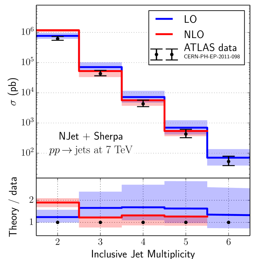
In Fig. 3 we show the data together with the theoretical predictions in leading and next-to-leading order. In case of the six jet rate only LO results are shown. In the lower plot the ratio of theoretical predictions with respect to data is given. With exception of the two jet cross section the inclusion of the NLO results improves significantly the comparison with data. For the higher multiplicities where NLO predictions are available the ratio between theory and data is about . Given that inclusive cross sections are intrinsically difficult to measure we consider this agreement as remarkable good. In particular for three-, four- and five-jet production the theoretical predictions agree within the uncertainties with the data. One should also keep in mind that a one per cent uncertainty of the collider energy may lead to sizeable changes in the cross sections. (For example, the inclusive cross section for top-quark pair production changes by about 3% when the energy is changed from 7 TeV to (70.07) TeV.) Instead of studying inclusive cross sections it is useful to consider their ratios since many theoretical and experimental uncertainties (i.e. uncertainties due to luminosity, scale dependence, PDF dependence etc.) may cancel between numerator and denominator. In particular one may consider
| (9) |
This quantity is in leading order proportional to the QCD coupling and can be used to determine the value of from jet rates.
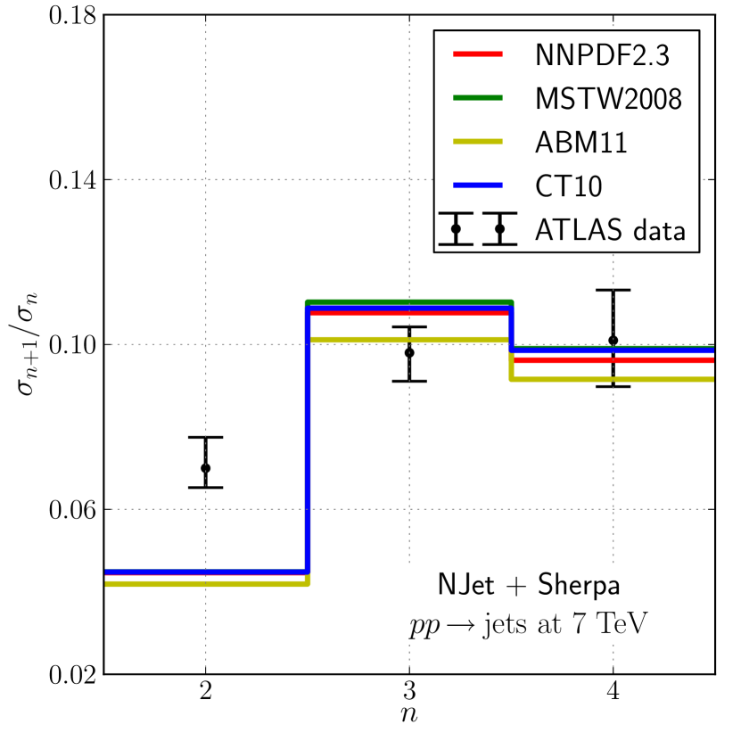
In Fig. 4 we show QCD predictions in NLO using different PDF sets together with the results from ATLAS. The results obtained from NNPDF2.3 are also collected in Tab. 3 where, in addition, the ratios at leading order (using the LO setup with NNPDF2.1) are shown.
| ATLASAad et al. (2011) | LO | NLO | |
|---|---|---|---|
| 2 | |||
| 3 | |||
| 4 | |||
| 5 |
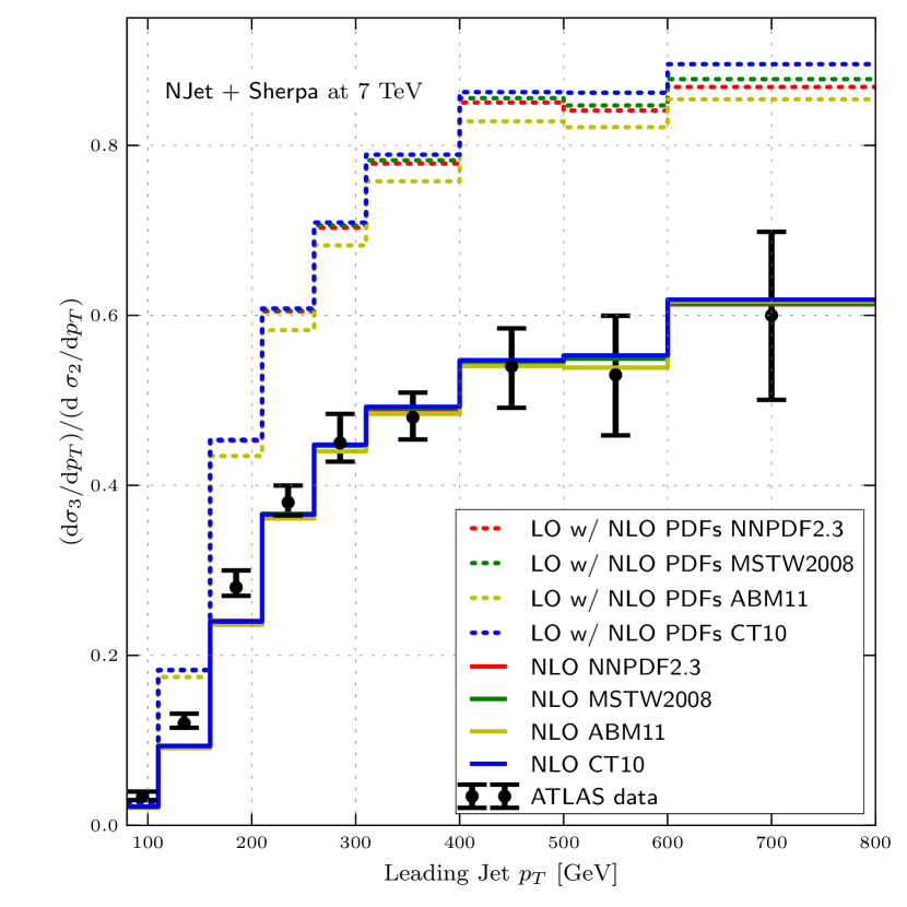
In case of and perturbation theory seems to provide stable results. The leading order and next-to-leading order values differ by less than 10%. In addition NNPDF Ball et al. (2013), CT10 Lai et al. (2010) and MSTW08 Martin et al. (2009) give compatible predictions. ABM11 Alekhin et al. (2012) gives slightly smaller results for and . Within uncertainties the predictions also agree with the ATLAS measurements. For a different picture is observed. First of all the theoretical predictions change by about % when going from LO to NLO. The origin of this behaviour is traced back to the inclusive two-jet cross section which is affected by large perturbative corrections. As a function of the leading jet , all PDF sets agree well with the 3/2 ratio ATLAS data at large as shown in figure Fig. 5.
In Fig. 6 we compare LO and NLO predictions for as function of the leading jet . While for and the corrections are moderate for all values of we observe large negative corrections independent from in case of .
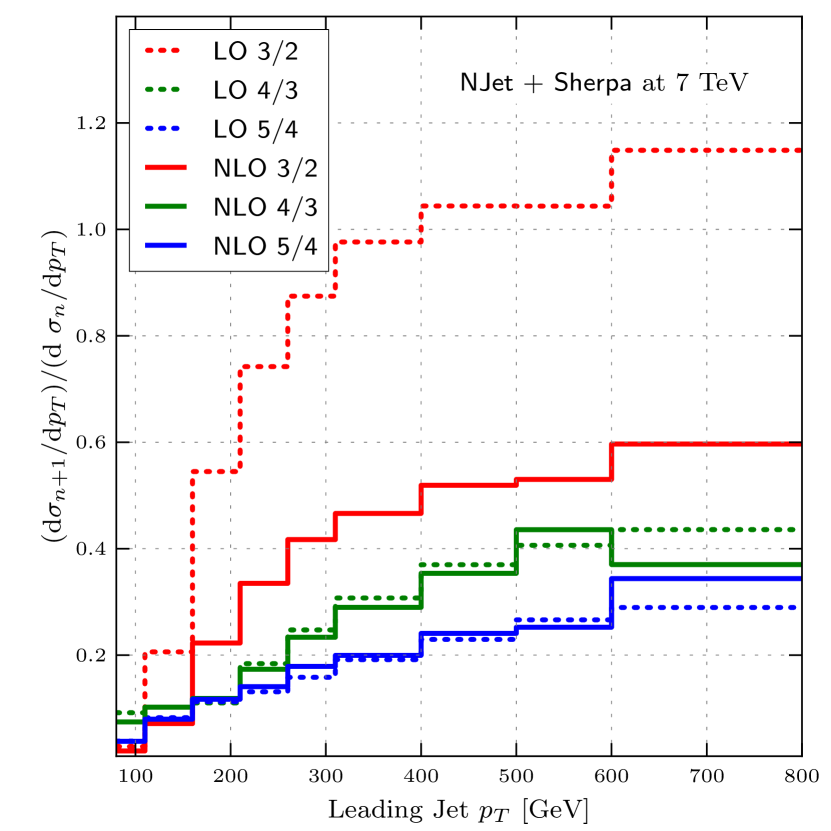
Most likely the two-jet rate is very sensitive to soft gluon emission while the higher jet multiplicities are less affected. As a consequence the fixed-order calculations fail to give reliable predictions for the 2-jet rate. A possible improvement could be expected from soft gluon resummation and matching with parton shower calculations. As long as only fixed-order calculations are used to predict we do not expect a perfect agreement with the data, especially in the low region. Similar to what has been observed in Fig. 3 the comparison with data shows indeed significant discrepancy in .
Let us now move on to less inclusive quantities.
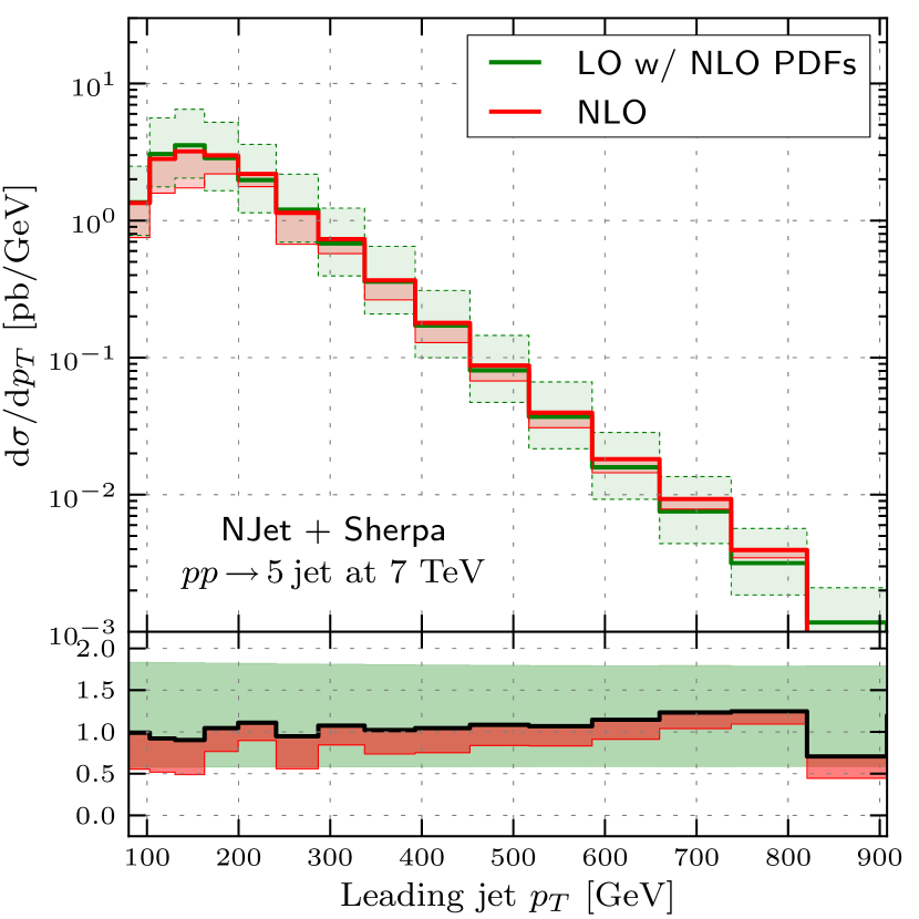
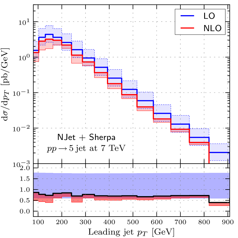
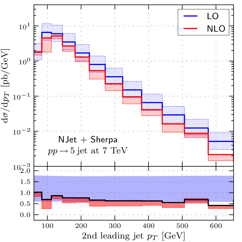
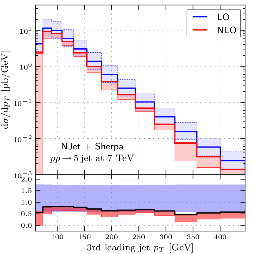
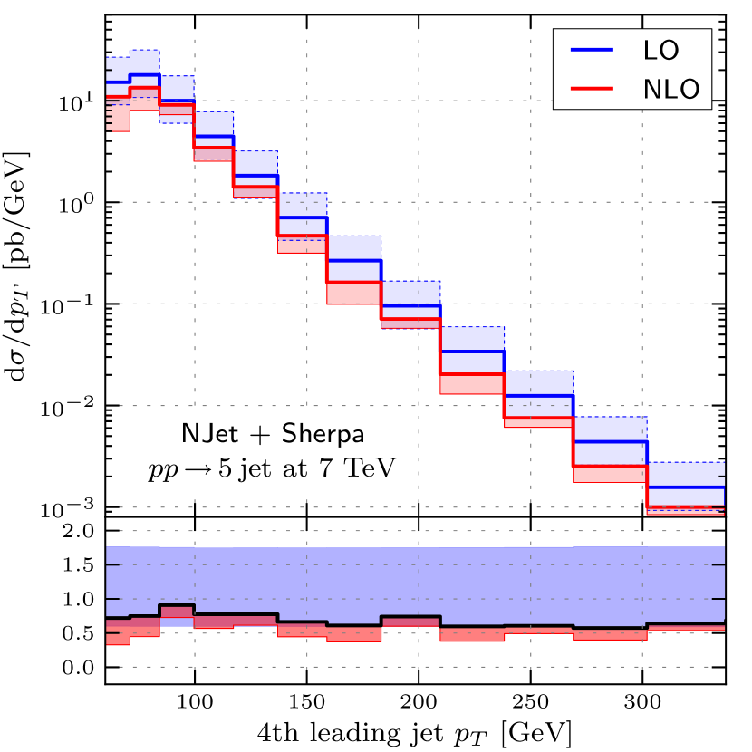
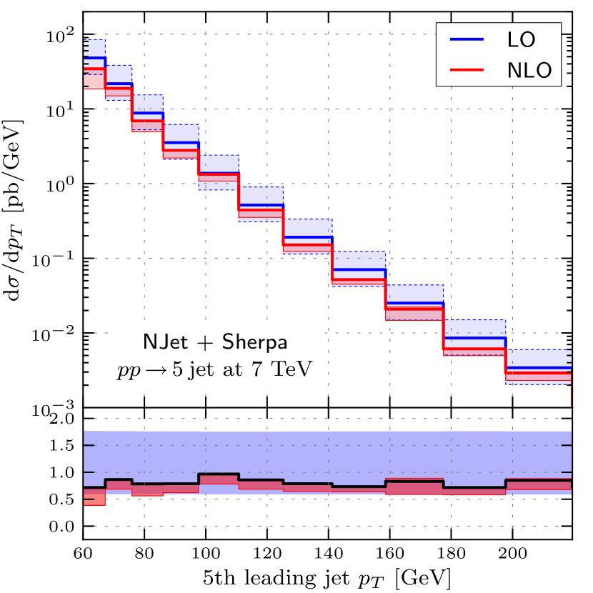
In Fig. 7 we show the transverse momentum distribution of the leading jet for five-jet production. Similar to the inclusive quantities a significant reduction of the scale uncertainty is observed when going from LO to NLO. Using again the NLO setup to calculate the LO predictions, the NLO calculation gives very small corrections. Over a wide range the LO predictions are modified by less than 10%. A remarkable feature observed already in the 4-jet calculation Bern et al. (2012); Badger et al. (2013b) is the almost constant K-factor. Again the dynamical scale seems to re-sum possible large logarithms which would appear at large transverse momentum using a fixed scale. Similar findings apply to transverse momentum distribution of the sub-leading jets.
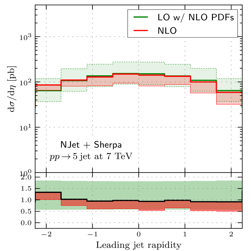
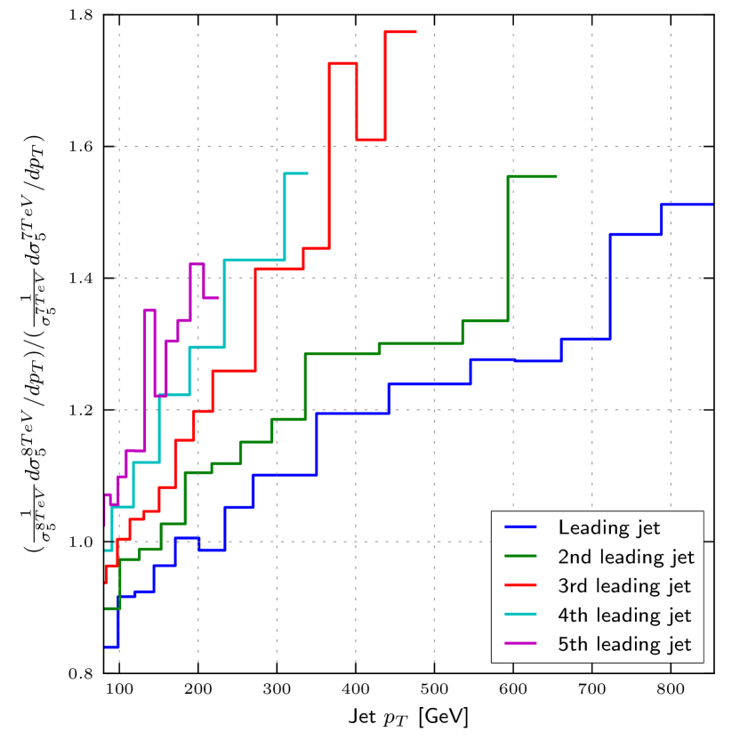
In Fig. 8 we show the rapidity distribution of the leading jet, again in LO and NLO QCD. In the range the distribution is remarkably flat. Again the NLO corrections are below 10% for most values and the K-factor is roughly constant. We have also investigated differential distributions for a centre-of-mass energy of 8 TeV. Studying normalized distributions to account for the increase of the inclusive jet cross section when going from 7 to 8 TeV we find a remarkable agreement between the 7 and 8 TeV predictions. As example we present in Fig. 9 the double-ratio,
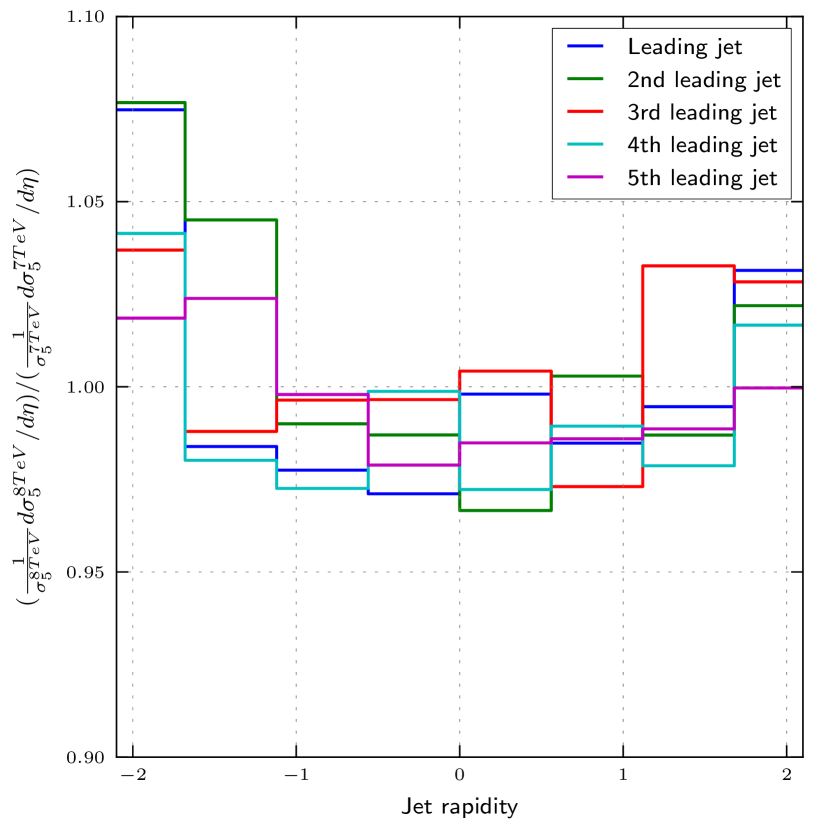
For simplicity we do not expand the double ratio in . Since the NLO corrections are moderate in size we do not expect a significant change in the prediction—the difference is formally of higher order in . As can be see in Fig. 9, the normalized rapidity distribution changes by less than 5% when going from 7 to 8 TeV. For the transverse momentum distribution we expect a harder spectrum for 8 TeV centre-of-mass energy compared to 7 TeV. This is indeed observed in Fig. 10. The fact that for low transverse momenta the ratios are below one is an effect of the normalization to the total cross section. For 8 TeV the regions where the inclusive cross section gets significant contributions is extended to larger leading to a ratio below one when comparing with the 7 TeV case.
Using data for jet production may provide useful input to constrain PDFs. In this context it is very interesting to study the decomposition of the jet rates with respect to individual partonic channels not only for inclusive quantities but also for differential distributions. In Fig. 11 the decomposition of the rapidity distribution of the leading jet is shown. As in the inclusive case we restrict the discussion to leading order.
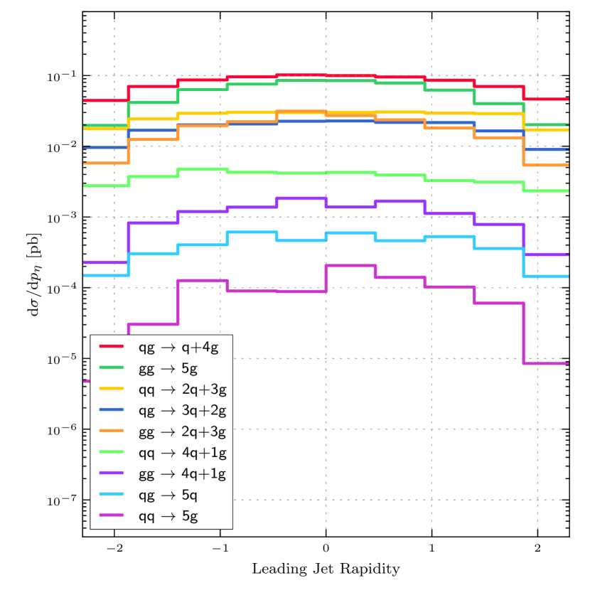
Evidently we find again that the channel is the most important channel followed by the pure gluonic channel. Since the rapidity distribution is only mildly affected by the partonic centre-of-mass energy we do not expect a strong dependence of the composition with respect to the rapidity. Indeed as can be seen from Fig. 11 the decomposition shows only a weak dependence on the rapidity. This information can be used to define control samples, when using jet data to constrain the parton luminosities.
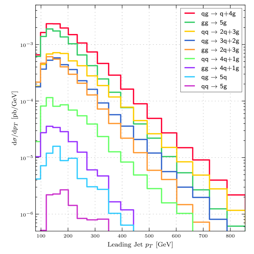
In Fig. 12 the analogous results for the transverse momentum distribution is presented. In difference to the rapidity distribution a significant dependence of the decomposition as function of the transverse momentum is visible. While at small transverse momentum the dominates over the situation changes at about 300 GeV and the becomes more important than . This behaviour is a direct consequence of the fact that at high partonic centre-of-mass energy the quark luminosity dominates over the gluon flux . A similar pattern, although less pronounced, can also be observed in the and channels. A cut in the transverse momentum can thus be used to change the mixture of the individual partonic channels and to provide additional information on specific parton luminosities. From the above discussion we expect that different PDF sets should give very similar results for the rapidity distribution since each bin is rather inclusive with respect to the partonic centre-of-mass energies where the luminosities are sampled. On the other hand if any difference using PDF sets from different groups is observed it will most likely show up in the transverse momentum distribution.
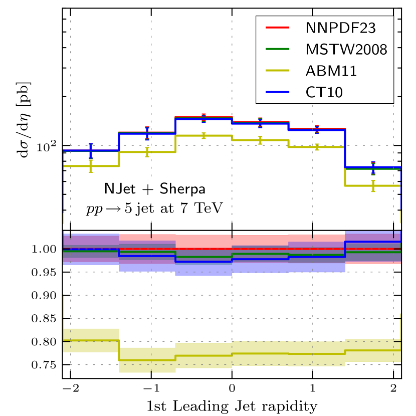
In Fig. 13 the rapidity distribution is shown using four different PDF sets. The PDF sets NNPDF2.3, CT10 and MSTW2008 lead to very similar results. A major difference is observed comparing the aforementioned PDF sets with ABM11. ABM11 leads to reduction of about 20% with respect to NNPDF2.3, CT10 and MSTW2008. However one can see that the shape for the distribution predicted by ABM11 agrees well with the other PDF sets. In Fig. 14 and Fig. 15 we show results for the normalized distributions.
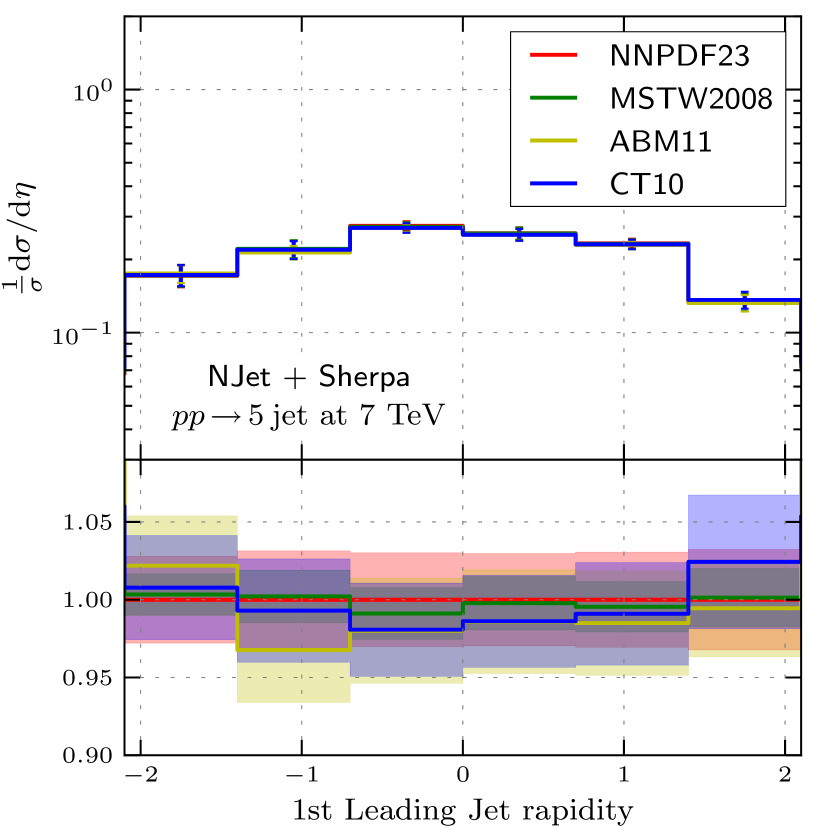
For the rapidity distribution the four different PDF sets agree well within %. The rapidity distributions of the sub leading jets show a similar behaviour.
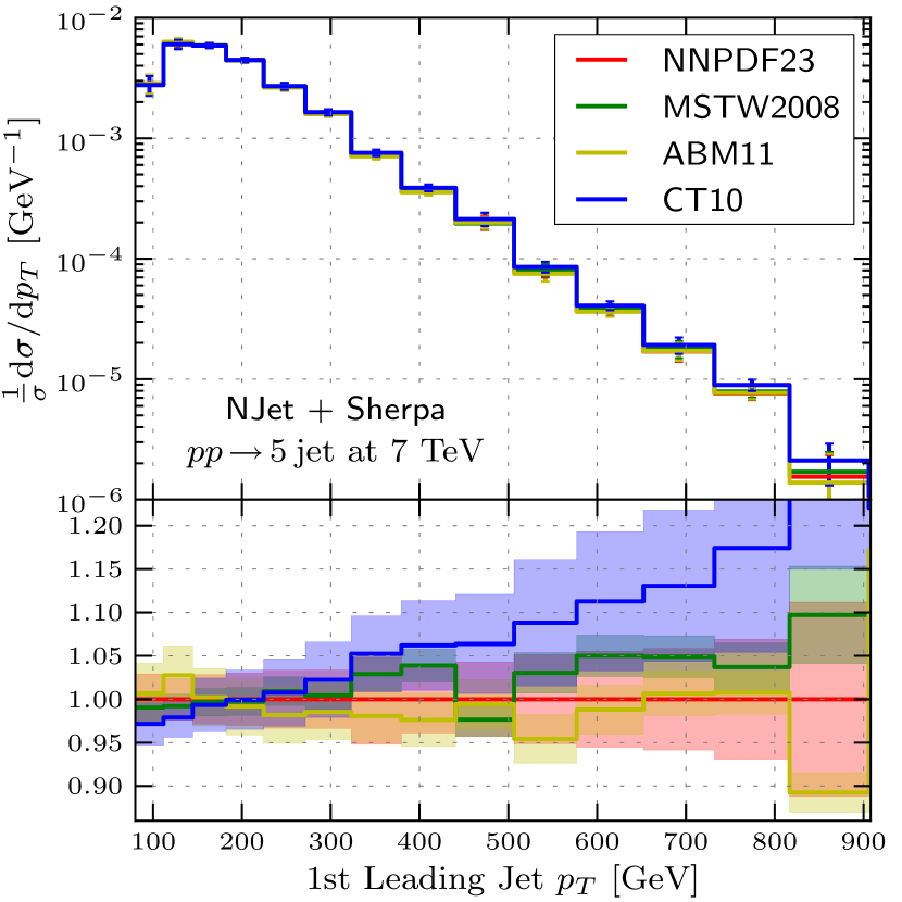
In Fig. 15 the transverse momentum distribution is studied for different PDF sets. As expected one can observe a richer structure at large transverse momentum. While minor differences are visible between ABM11, MSTW08 and NNPDF they still give rather similar results at large at the level of %. However the CT10 PDF set leads to significantly larger results at large . In the highest bin the normalised cross section is enhanced by about % compared to ABM11, MSTW08 and NNPDF. Unfortunately it is not easy to distinguish the different predictions experimentally since the cross section for this bin is reduced by several orders of magnitude. A significant amount of data is thus required to achieve the required statistical sensitivity.
IV Conclusions
In this article we have presented first results for five-jet production at NLO accuracy in QCD. We find moderate corrections at NLO with respect to a leading order computation using NLO PDFs. Typically corrections of the order of 10% are observed. Identifying renormalization and factorization scale and using the total transverse momentum as dynamical scale leads to a flat K-factor for the differential distributions. We have compared theoretical predictions for inclusive jet cross sections and jet rates with data from ATLAS. With the exception of quantities affected by the two jet rate we find good agreement between theory and data. As a major uncertainty of the theoretical predictions we have investigated the impact of using different PDF sets. While for rather inclusive quantities and distributions not sensitive to a specific partonic centre-of-mass energy good agreement of different sets is observed (in case of distributions this requires to study normalized predictions) significant differences are observed in the transverse momentum distribution of the leading jet at large momentum.
The analysis of the jet ratios shows that the and predictions appear to be perturbatively more stable than the predictions with modest correction at NLO. This indicates that these quantities are good candidates for future extractions of from the LHC data, where reliable fixed order predictions are mandatory. We hope the results presented here will be useful in these and other analyses in the future.
Acknowledgements
This work is supported by the Helmholtz Gemeinschaft under contract HA-101 (Alliance Physics at the Terascale), by the German Research Foundation (DFG) through the transregional collaborative research centre “Computational Particle Physics” (SFB-TR9) and by the European Commission through contract PITN-GA-2010-264564 (LHCPhenoNet). We would also like to thank DESY Zeuthen theory group for providing computer resources.
Appendix A Differential distributions for sub-leading jets
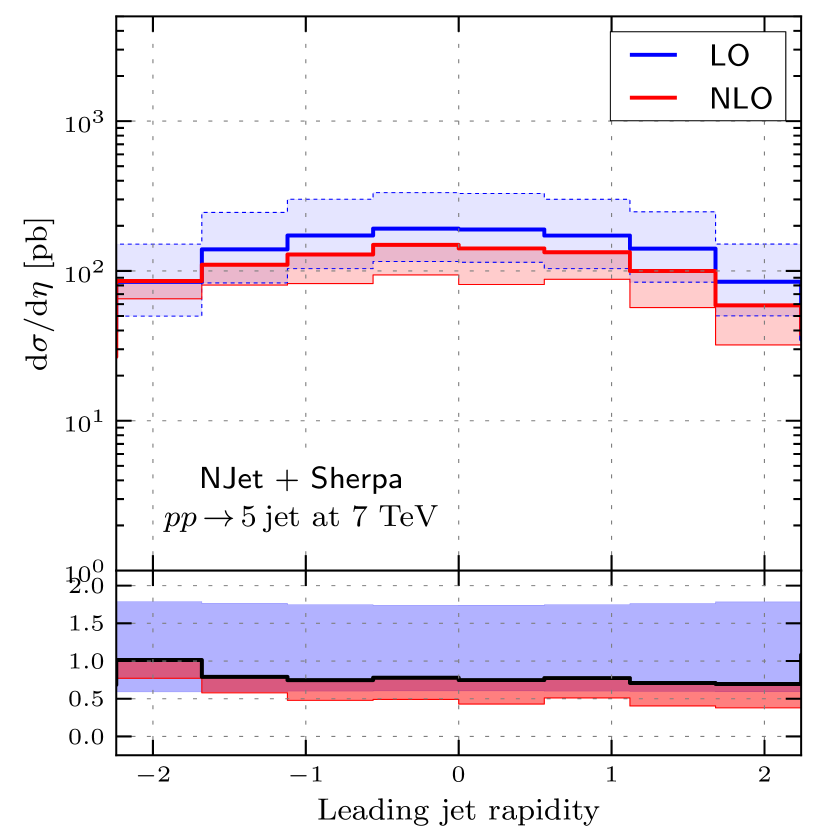
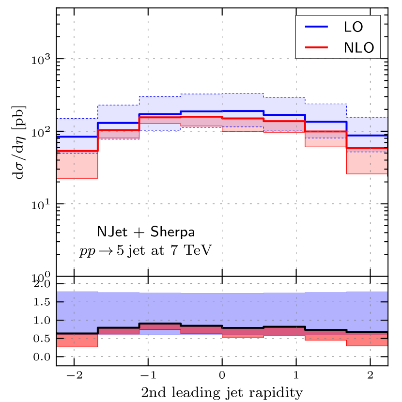
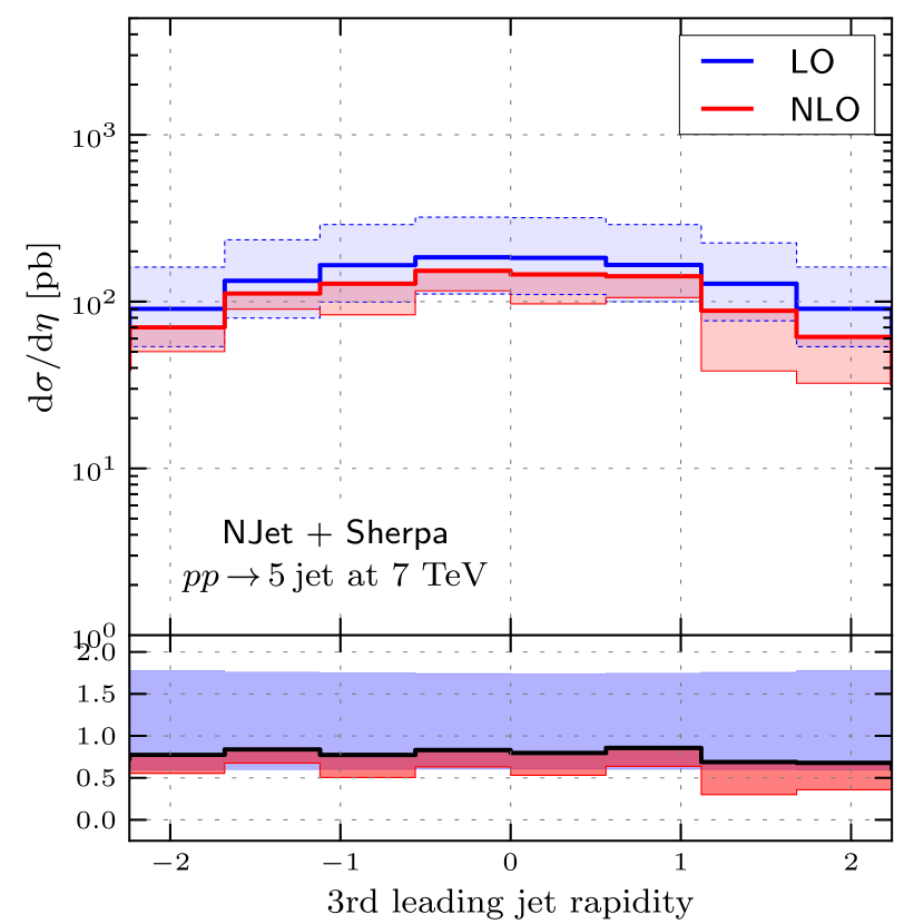
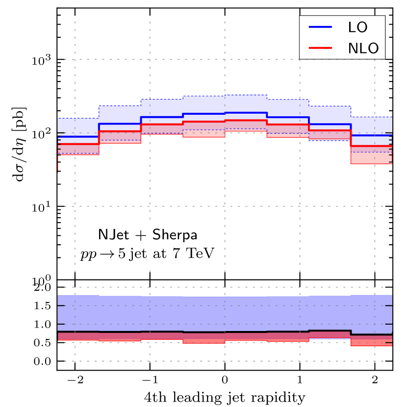
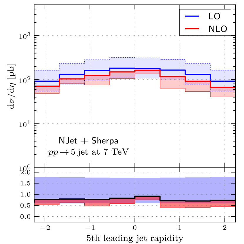
In this appendix we present all rapidity and distributions for jets ordered in . A complete set of histograms and plots for and TeV can be obtained from https://bitbucket.org/njet/njet/wiki/Results/Physics.
Appendix B Numerical results for differential distributions
We provide numerical values for the histograms in figures 7 and 8 in tables 4 and 5 for ease of future comparisons.
| (GeV) | LO (pb) | NLO (pb) |
|---|---|---|
| — | ||
| — | ||
| — | ||
| — | ||
| — | ||
| — | ||
| — | ||
| — | ||
| — | ||
| — | ||
| — | ||
| — | ||
| — | ||
| — | ||
| — | ||
| — | ||
| — | ||
| — | ||
| — | ||
| — |
| (GeV) | LO (pb) | NLO (pb) |
|---|---|---|
| — | ||
| — | ||
| — | ||
| — | ||
| — | ||
| — | ||
| — | ||
| — | ||
| — | ||
| — |
References
- Badger et al. (2013a) S. Badger, B. Biedermann, P. Uwer, and V. Yundin, Comput.Phys.Commun. 184, 1981 (2013a), arXiv:1209.0100 [hep-ph] .
- Giele et al. (1993) W. Giele, E. N. Glover, and D. A. Kosower, Nucl.Phys. B403, 633 (1993), arXiv:hep-ph/9302225 [hep-ph] .
- Nagy (2002) Z. Nagy, Phys.Rev.Lett. 88, 122003 (2002), arXiv:hep-ph/0110315 [hep-ph] .
- Kilgore and Giele (1997) W. B. Kilgore and W. Giele, Phys.Rev. D55, 7183 (1997), arXiv:hep-ph/9610433 [hep-ph] .
- Bern et al. (2012) Z. Bern, G. Diana, L. Dixon, F. Febres Cordero, S. Hoeche, et al., Phys.Rev.Lett. 109, 042001 (2012), arXiv:1112.3940 [hep-ph] .
- Badger et al. (2013b) S. Badger, B. Biedermann, P. Uwer, and V. Yundin, Phys.Lett. B718, 965 (2013b), arXiv:1209.0098 [hep-ph] .
- Aad et al. (2011) G. Aad et al. (ATLAS Collaboration), Eur.Phys.J. C71, 1763 (2011), arXiv:1107.2092 [hep-ex] .
- Alioli et al. (2011) S. Alioli, K. Hamilton, P. Nason, C. Oleari, and E. Re, JHEP 1104, 081 (2011), arXiv:1012.3380 [hep-ph] .
- Hoeche and Schonherr (2012) S. Hoeche and M. Schonherr, (2012), arXiv:1208.2815 [hep-ph] .
- Ridder et al. (2013) A. G.-D. Ridder, T. Gehrmann, E. Glover, and J. Pires, Phys.Rev.Lett. 110, 162003 (2013), arXiv:1301.7310 [hep-ph] .
- Badger et al. (2011) S. Badger, B. Biedermann, and P. Uwer, Comput.Phys.Commun. 182, 1674 (2011), arXiv:1011.2900 [hep-ph] .
- Hirschi et al. (2011) V. Hirschi, R. Frederix, S. Frixione, M. V. Garzelli, F. Maltoni, et al., JHEP 1105, 044 (2011), arXiv:1103.0621 [hep-ph] .
- Bevilacqua et al. (2011) G. Bevilacqua, M. Czakon, M. Garzelli, A. van Hameren, A. Kardos, et al., (2011), arXiv:1110.1499 [hep-ph] .
- Cullen et al. (2012) G. Cullen, N. Greiner, G. Heinrich, G. Luisoni, P. Mastrolia, et al., Eur.Phys.J. C72, 1889 (2012), arXiv:1111.2034 [hep-ph] .
- Cascioli et al. (2012) F. Cascioli, P. Maierhofer, and S. Pozzorini, Phys.Rev.Lett. 108, 111601 (2012), arXiv:1111.5206 [hep-ph] .
- Becker et al. (2012) S. Becker, D. Goetz, C. Reuschle, C. Schwan, and S. Weinzierl, Phys.Rev.Lett. 108, 032005 (2012), arXiv:1111.1733 [hep-ph] .
- Actis et al. (2013) S. Actis, A. Denner, L. Hofer, A. Scharf, and S. Uccirati, JHEP 1304, 037 (2013), arXiv:1211.6316 [hep-ph] .
- Bevilacqua and Worek (2012) G. Bevilacqua and M. Worek, JHEP 1207, 111 (2012), arXiv:1206.3064 [hep-ph] .
- Bern et al. (2013) Z. Bern, L. Dixon, F. Febres Cordero, S. Hoeche, H. Ita, et al., Phys.Rev. D88, 014025 (2013), arXiv:1304.1253 [hep-ph] .
- Cullen et al. (2013) G. Cullen, H. van Deurzen, N. Greiner, G. Luisoni, P. Mastrolia, et al., (2013), arXiv:1307.4737 [hep-ph] .
- van Deurzen et al. (2013) H. van Deurzen, G. Luisoni, P. Mastrolia, E. Mirabella, G. Ossola, et al., (2013), arXiv:1307.8437 [hep-ph] .
- Gehrmann et al. (2013) T. Gehrmann, N. Greiner, and G. Heinrich, (2013), arXiv:1308.3660 [hep-ph] .
- Alcaraz Maestre et al. (2012) J. Alcaraz Maestre et al. (SM AND NLO MULTILEG and SM MC Working Groups), (2012), arXiv:1203.6803 [hep-ph] .
- Bern et al. (1994) Z. Bern, L. J. Dixon, D. C. Dunbar, and D. A. Kosower, Nucl.Phys. B425, 217 (1994), arXiv:hep-ph/9403226 [hep-ph] .
- Bern et al. (1995) Z. Bern, L. J. Dixon, D. C. Dunbar, and D. A. Kosower, Nucl.Phys. B435, 59 (1995), arXiv:hep-ph/9409265 [hep-ph] .
- Gleisberg et al. (2009) T. Gleisberg, S. Hoeche, F. Krauss, M. Schonherr, S. Schumann, et al., JHEP 0902, 007 (2009), arXiv:0811.4622 [hep-ph] .
- Gleisberg and Hoeche (2008) T. Gleisberg and S. Hoeche, JHEP 0812, 039 (2008), arXiv:0808.3674 [hep-ph] .
- Gleisberg and Krauss (2008) T. Gleisberg and F. Krauss, Eur.Phys.J. C53, 501 (2008), arXiv:0709.2881 [hep-ph] .
- Catani and Seymour (1996) S. Catani and M. Seymour, Phys.Lett. B378, 287 (1996), arXiv:hep-ph/9602277 [hep-ph] .
- Britto et al. (2005) R. Britto, F. Cachazo, and B. Feng, Nucl.Phys. B725, 275 (2005), arXiv:hep-th/0412103 [hep-th] .
- Ellis et al. (2008) R. Ellis, W. Giele, and Z. Kunszt, JHEP 0803, 003 (2008), arXiv:0708.2398 [hep-ph] .
- Forde (2007) D. Forde, Phys.Rev. D75, 125019 (2007), arXiv:0704.1835 [hep-ph] .
- Berger et al. (2008) C. Berger, Z. Bern, L. Dixon, F. Febres Cordero, D. Forde, et al., Phys.Rev. D78, 036003 (2008), arXiv:0803.4180 [hep-ph] .
- Ossola et al. (2007) G. Ossola, C. G. Papadopoulos, and R. Pittau, Nucl.Phys. B763, 147 (2007), arXiv:hep-ph/0609007 [hep-ph] .
- Giele et al. (2008) W. T. Giele, Z. Kunszt, and K. Melnikov, JHEP 0804, 049 (2008), arXiv:0801.2237 [hep-ph] .
- Badger (2009) S. Badger, JHEP 0901, 049 (2009), arXiv:0806.4600 [hep-ph] .
- Berends and Giele (1988) F. A. Berends and W. T. Giele, Nucl. Phys. B306, 759 (1988).
- van Oldenborgh (1991) G. van Oldenborgh, Comput.Phys.Commun. 66, 1 (1991).
- Ellis and Zanderighi (2008) R. K. Ellis and G. Zanderighi, JHEP 0802, 002 (2008), arXiv:0712.1851 [hep-ph] .
- Binoth et al. (2010) T. Binoth, F. Boudjema, G. Dissertori, A. Lazopoulos, A. Denner, et al., Comput.Phys.Commun. 181, 1612 (2010), dedicated to the memory of, and in tribute to, Thomas Binoth, who led the effort to develop this proposal for Les Houches 2009, arXiv:1001.1307 [hep-ph] .
- Alioli et al. (2013) S. Alioli, S. Badger, J. Bellm, B. Biedermann, F. Boudjema, et al., (2013), arXiv:1308.3462 [hep-ph] .
- Cacciari et al. (2012) M. Cacciari, G. P. Salam, and G. Soyez, Eur.Phys.J. C72, 1896 (2012), arXiv:1111.6097 [hep-ph] .
- Cacciari et al. (2008) M. Cacciari, G. P. Salam, and G. Soyez, JHEP 0804, 063 (2008), arXiv:0802.1189 [hep-ph] .
- Whalley et al. (2005) M. Whalley, D. Bourilkov, and R. Group, (2005), arXiv:hep-ph/0508110 [hep-ph] .
- Ball et al. (2012) R. D. Ball et al. (NNPDF Collaboration), Nucl.Phys. B855, 153 (2012), arXiv:1107.2652 [hep-ph] .
- Ball et al. (2013) R. D. Ball, V. Bertone, S. Carrazza, C. S. Deans, L. Del Debbio, et al., Nucl.Phys. B867, 244 (2013), arXiv:1207.1303 [hep-ph] .
- Andersen et al. (2010) J. Andersen et al. (SM and NLO Multileg Working Group), , 21 (2010), arXiv:1003.1241 [hep-ph] .
- Lai et al. (2010) H.-L. Lai, M. Guzzi, J. Huston, Z. Li, P. M. Nadolsky, et al., Phys.Rev. D82, 074024 (2010), arXiv:1007.2241 [hep-ph] .
- Martin et al. (2009) A. Martin, W. Stirling, R. Thorne, and G. Watt, Eur.Phys.J. C63, 189 (2009), arXiv:0901.0002 [hep-ph] .
- Alekhin et al. (2012) S. Alekhin, J. Blumlein, and S. Moch, (2012), arXiv:1202.2281 [hep-ph] .