What controls the large-scale magnetic fields of M dwarfs?

Abstract

Observations of active M dwarfs show a broad variety of large-scale magnetic fields encompassing dipole-dominated and multipolar geometries. We detail the analogy between some anelastic dynamo simulations and spectropolarimetric observations of 23 M stars. In numerical models, the relative contribution of inertia and Coriolis force –estimated by the so-called local Rossby number– is known to have a strong impact on the magnetic field geometry. We discuss the relevance of this parameter in setting the large-scale magnetic field of M dwarfs.

1 Introduction

The magnetic fields of planets and rapidly-rotating stars are maintained by convection-driven dynamos operating in their interiors. Scaling laws recently derived from geodynamo-like models successfully predict the magnetic field strength of a wide range of astrophysical objects from Earth and Jupiter to some rapidly-rotating stars [Christensen & Aubert (2006), Christensen (2010), Yadav et al. (2013), Yadav et al. (2013), (e.g. Christensen & Aubert 2006; Christensen et al. 2009; Yadav et al. 2013a,b)]. This emphasises the similarities between the dynamo mechanisms at work in planets and active M dwarfs.

Spectropolarimetric observations of rapidly-rotating M stars show a broad variety of large-scale magnetic fields encompassing dipole-dominated and multipolar geometries [Donati et al. (2008), Morin et al. (2008a), Morin et al. (2008b), Morin et al. (2010), (Donati et al. 2008; Morin et al. 2008a,b,2010)]. Combining global-scale numerical dynamo models and observational results, we want to better understand the similarities of dynamos in planets and low-mass stars. To study the physical mechanisms that control the magnetic field morphology in these objects, we have explored the influence of rotation rate, convective vigor and density stratification on the magnetic field properties in anelastic dynamo models [Gastine et al. (2012), Gastine et al. (2013), (Gastine et al. 2012,2013)].

In such models, the relative importance of inertia and Coriolis force in the force balance –quantified by the local Rossby number $Ro_{l}$– is thought to have a strong impact on the magnetic field geometry [Christensen & Aubert (2006), (Christensen & Aubert 2006)]. A sharp transition between dipole-dominated and multipolar dynamos is indeed observed at $Ro_{l}\simeq 0.1$. However, [Simitev & Busse (2009)] find that both dipolar and multipolar magnetic fields are two possible solutions at the same parameter regime, depending on the initial condition of the system. As shown by [Schrinner et al. (2012)], this dynamo bistability challenges the $Ro_{l}$ criterion as the multipolar dynamo branch can extend well below the threshold value $Ro_{l}\simeq 0.1$.

Here we discuss the analogy between the anelastic dynamo models by [Gastine et al. (2012)] and the spectropolarimetric observations of 23 M stars. The reader is referred to [Gastine et al. (2013), (Gastine et al. 2013)] for a more comprehensive description of the results.

2 Dynamo models and spectropolarimetric observations

We consider MHD simulations of a conducting anelastic fluid in spherical shells rotating at a constant rotation rate $\Omega$. A fixed entropy contrast $\Delta s$ between the inner and the outer boundary drives the convective motions. Our numerical models are computed using the anelastic spectral code MagIC [Wicht (2002), Gastine & Wicht (2012), (Wicht 2002, Gastine & Wicht 2012)] that has been validated against several hydrodynamical and dynamo benchmarks [Jones et al. (2011), (Jones et al. 2011)]. The governing MHD equations are non-dimensionalised using the shell thickness $d=r_{o}-r_{i}$ as the reference lengthscale and $\Omega^{-1}$ as the time unit.

The solution of a numerical model is then characterised by several diagnostic parameters. The rms flow velocity is given by the Rossby number $Ro=u_{\text{rms}}/\Omega d$, while the magnetic field strength is measured by the Elsasser number $\Lambda=B_{\text{rms}}^{2}/\rho\mu\lambda\Omega$, where $\rho$ is the density, and $\mu$ and $\lambda$ are the magnetic permeability and diffusivity. The typical flow lengthscale $l$ is defined as $l=\pi d/\bar{\ell}_{u}$, where $\bar{\ell}_{u}$ is the mean spherical harmonic degree obtained from the kinetic energy spectrum [Christensen & Aubert (2006), Schrinner et al. (2012), (Christensen & Aubert 2006; Schrinner et al. 2012)]. Following [Christensen & Aubert (2006)], a local Rossby number $Ro_{l}=u_{\text{rms}}/\Omega l$, can then be used to evaluate the impact of inertia on the magnetic field geometry. Finally, the geometry of the surface magnetic field is quantified by its dipolarity $f_{\text{dip}}=\mathchoice{\mbox{\boldmath$\displaystyle B$}}{\mbox{\boldmath$\textstyle B$}}{\mbox{\boldmath$\scriptstyle B$}}{\mbox{\boldmath$\scriptscriptstyle B$}}_{\ell=1,m=0}^{2}(r=r_{o})/\sum_{\ell,m}^{\ell_{\text{max}}}\mathchoice{\mbox{\boldmath$\displaystyle B$}}{\mbox{\boldmath$\textstyle B$}}{\mbox{\boldmath$\scriptstyle B$}}{\mbox{\boldmath$\scriptscriptstyle B$}}_{\ell,m}^{2}(r=r_{o})$, the ratio of the magnetic energy of the dipole to the magnetic energy contained in spherical harmonic degrees up to $\ell_{\text{max}}=11$.

We compare these dynamo models with spectropolarimetric observations of 23 active M dwarfs with rotation period ranging from 0.4 to 19 days. The data reduction and analysis is detailed by [Donati et al. (2006)] and [Morin et al. (2008a), Morin et al. (2008b), Morin et al. (2010), Morin et al. (2008a,b,2010)]. We derive observation-based quantities aimed to reflect the diagnostic parameters employed in the numerical models. The empirical Rossby number $Ro_{\text{emp}}=P_{\text{rot}}/\tau_{c}$ is our best available proxy for $Ro_{l}$, where $\tau_{c}$ is the turnover timescale of convection based on the rotation-activity relation [Kiraga & Stepien(2007), (Kiraga & Stepien 2007)]. We define an Elsasser number based on the averaged unsigned large-scale magnetic field $\left\langle\rm B_{\rm V}\right\rangle$ that roughly characterises the ratio between Lorentz and Coriolis forces. We also consider the fraction of the magnetic energy that is recovered in the axial dipole mode in Zeeman-Doppler imaging maps [Semel (1989), (ZDI, Semel 1989)]. The spatial resolution of such maps mostly depends on the projected rotational velocity $v\sin i$. The actual degree and order $\ell_{\text{max}}$ up to which the reconstruction can be performed ranges from 4 to 10. We directly compare this quantity to the dipolarity employed in numerical models and term them both $f_{\text{dip}}$ in Figs. 1-2.

3 Results and discussion

Figure 1: $f_{\text{dip}}$ plotted against $Ro_{l}$ in the anelastic dynamo models computed by [Gastine et al. (2012)]. Red (grey) symbols correspond to numerical simulations in thick (thin) shells ($r_{i}/r_{o}=0.2$ and $r_{i}/r_{o}=0.6$). The symbol sizes scale with the amplitude of the surface field, given in units of the square-root of the Elsasser number. The two vertical lines mark the possible upper-limits of the dipole-dominated dynamos. The two filled symbols are further discussed in Fig. 3.

Figure 2: $f_{\text{dip}}$ plotted against $Ro_{\text{emp}}$. The symbol sizes scale with the square root of the Elsasser number based on the large-scale magnetic field derived from spectropolarimetric observations. The vertical dashed line marks the possible upper bound of the dipolar regime. For the two stars with the largest temporal variation, individual epochs are connected by a vertical red line. Dotted red circles with errorbars correspond to some stars from [Morin et al. (2010)] for which a definite ZDI reconstruction was not possible.

Figure 3: Snapshot of the radial component of the surface magnetic field and the axisymmetric zonal flow $\bar{u}_{\phi}$ for a dipolar dynamo model (a), and a multipolar case (b). Magnetic field are given in units of the square root of the Elsasser number and velocities in units of the Rossby number.

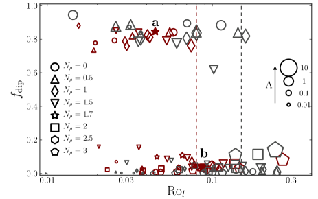
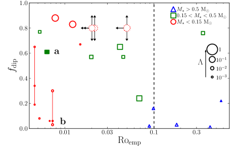
Figure 1 shows $f_{\text{dip}}$ versus $Ro_{l}$ in the numerical models, while Fig. 2 displays the relative dipole strength of M stars against $Ro_{\text{emp}}$ derived from spectropolarimetric observations. The numerical models cluster in two distinct dynamo branches: the upper branch corresponds to the dipole-dominated regime ($f_{\text{dip}}>0.6$), while the lower branch contains the multipolar dynamos ($f_{\text{dip}}<0.2$). Fig. 3 shows two selected cases of these two kinds of dynamo action. The dipolar branch is limited by a maximum $Ro_{l}\simeq 0.1$, beyond which all the models become multipolar. In contrast to earlier Boussinesq studies [Christensen & Aubert (2006), (e.g. Christensen & Aubert 2006)], the multipolar branch also extends well below $Ro_{l}\simeq 0.1$, where both dipolar and multipolar solutions are stable [Schrinner et al. (2012), (see Schrinner et al. 2012)]. Bistability of the magnetic field is in fact quite common in the parameter range explored here, meaning that both dipole-dominated and multipolar fields are two possible stable configurations at the same set of parameters [Simitev & Busse (2009), (Simitev & Busse 2009)]. The multipolar branch at low $Ro_{l}$ is partly composed by the anelastic models with $\rho_{\text{bot}}/\rho_{\text{top}}>7$ [Gastine & Wicht (2012), (Gastine et al. 2012)] and partly by the multipolar attractors of these bistable cases. Note that different assumptions in the numerical models (for instance variable transport properties) help to extend the dipolar regime towards higher density contrasts [Duarte et al. (2013), (Duarte et al. 2013)].

Although it is difficult to directly relate the diagnostic parameters employed in numerical models to their observational counterparts, the separation into two dynamo branches seems to be relevant to the sample of active M dwarfs displayed in Fig. 2. In particular, the late M dwarfs (with $M_{\star}<0.15\,\text{M}_{\odot}$) seem to operate in two different dynamo regimes: the first ones show a strong dipolar field, while others present a weaker multipolar magnetic field with a pronounced time-variability.

This analogy between numerical models and observations of active M dwarfs could be further assessed by additional observations. Indeed, if the analogy holds, stars with a multipolar field are expected over a continuous range of Rossby number where dipole-dominated large-scale fields are also observed (i.e. $0.01<Ro_{\text{emp}}<0.1$).