11institutetext: Qiyu JIN 22institutetext: Institute of Image Processing and Pattern Recognition, Shanghai Jiao Tong University, No. 800 Dongchuan Road, Minhang District, Shanghai 200240, China
UMR 6205, Laboratoire de Math matiques de Bretagne Atlantique, Université de Bretagne-Sud, Campus de Tohaninic, BP 573, 56017 Vannes, France
Université Européenne de Bretagne, France
Jiangsu Engineering Center of Network Monitoring, Nanjing University of Information Science &\& Technology, Nanjing 210044, China
22email: qiyu.jin2008@gmail.com
33institutetext: Ion Grama 44institutetext: UMR 6205, Laboratoire de Math matiques de Bretagne Atlantique, Université de Bretagne-Sud, Campus de Tohaninic, BP 573, 56017 Vannes, France
Université Européenne de Bretagne, France
44email: ion.grama@univ-ubs.fr
55institutetext: Quansheng Liu 66institutetext: UMR 6205, Laboratoire de Math matiques de Bretagne Atlantique, Université de Bretagne-Sud, Campus de Tohaninic, BP 573, 56017 Vannes, France
Université Européenne de Bretagne, France
School of Mathematics and Computing Sciences, Changsha University of Science and Technology, Changsha 410076, China
66email: quansheng.liu@univ-ubs.fr

A Non-Local Means Filter for Removing the Poisson Noise

Qiyu JIN    Ion Grama    Quansheng Liu
Abstract

A new image denoising algorithm to deal with the Poisson noise model is given, which is based on the idea of Non-Local Mean. By using the ”Oracle” concept, we establish a theorem to show that the Non-Local Means Filter can effectively deal with Poisson noise with some modification. Under the theoretical result, we construct our new algorithm called Non-Local Means Poisson Filter and demonstrate in theory that the filter converges at the usual optimal rate. The filter is as simple as the classic Non-Local Means and the simulation results show that our filter is very competitive.

Keywords:
Non-Local MeansMean Square ErrorPoisson noise”Oracle” estimator

1 Introduction

Noise is inevitable in any image device. A digital imaging system consists of an optical system followed by a photodetector and associated electrical filters. The photodetector converts the incident optical intensity to a detector current, i.e. photons to electrons. During the process, the true signals are contaminated by many different sources of noise. The Poisson noise appears in low-light conditions when the number of collected photons is small, such as night vision, medical imaging, underwater imaging, microscopic imaging, optical microscopy imaging and astronomy imaging. Such a noise is signal-dependent, and requires to adapt the usual denoising approaches.

The key challenge in Poisson intensity estimation problems is that the variances of the observed counts are different. As a result, many methods are introduced to transform the Poisson distributed noise to the data approximately Gaussian and homoscedastic. These methods are called Variance Stabilizing Transformations (VST), such as Anscombe root transformation (1948 ANSCOMBE1948TRANSFORMATION , and 1993 borovkov2000estimates ), multiscal VSTs (2008 ZHANG2008WAVELETS ), conditional variance stabilization (CVS) (2006 jansen2006multiscale ), or Haar-Fisz transformation (2004 FRYZLEWICZ2004HAAR and 2007 FRYZLEWICZ2007GOES ). Then we can deal with these data as Gaussian noise. Second, the noise is removed using a conventional denoising algorithm for additive white Gaussian noise, see for example Buades, Coll and Morel (2005 buades2005review ), Kervrann (2006 kervrann2006optimal ), Aharon and Elad and Bruckstein (2006 aharon2006rm ), Hammond and Simoncelli (2008 hammond2008image ), Polzehl and Spokoiny (2006 polzehl2006propagation ), Hirakawa and Parks (2006 hirakawa2006image ), Mairal, Sapiro and Elad (2008 mairal2008learning ), Portilla, Strela, Wainwright and Simoncelli (2003 portilla2003image ), Roth and Black (2009 roth2009fields ), Katkovnik, Foi, Egiazarian, and Astola (2010 Katkovnik2010local ), Dabov, Foi, Katkovnik and Egiazarian (2006 buades2009note ), Abraham, Abraham, Desolneux and Li-Thiao-Te (2007 Abraham2007significant ), and Jin, Grama and Liu (2011 JinGramaLiuowf ). After denoising, some inverse transformations, like Exact Unbiased Inverse (EUI) (2009 MAKITALO2009INVERSION and 2011 makitalo2011optimal ), are applied to the denoised signal, obtaining the estimate of the signal of interest. Many authors restore the Poisson noise by this type of methods with a three-step procedure (see boulanger2008non ; ZHANG2008WAVELETS ; lefkimmiatis2009bayesian ; luisier2010fast ).

Maxmum Likelihood (ML) estimation (1996 van1996comparing , 2009moon2009three ) and Similarity Measure (SM) (2006 alter2006intensity ) are also found to be effective since they can account for the special properties of the Poisson distribution. Others methods like as Complexity-Penalized Likelihood Estimation (CPLE) (2000 nowak2000statistical , 2005 kolaczyk2005multiscale ) and Total Variation (TV) seminorm (2009 beck2009fast ), have been introduced to deal with the Poisson noise. Le et al. ((le2007variational, )) have adapted the successful ROF model for total variation regularization to deal with Poisson noise. The gradient descent iteration for this model replaces the regularization parameter with a function.

The Non-Local Means Filter has been proposed by Buades et al (2005 buades2005review ) to denoise images damaged by additive white Gaussian noise. It is based on the similarity phenomenon existing very often in natural images, and assumes that there is enough redundant information (pixels having identical noise-free value) in the image to reduce the noise significantly. This filter is known to efficiently reduce the noise and to preserve structures. Some authors (see 2008 boulanger2008non , 2010 deledalle2010poisson ) combine the Non-Local Means method with other methods to restore the Poisson noise. Deledalle et al. (2010 (deledalle2010poisson, )) proposed an extension of the Non-Local Means for images damaged by Poisson noise. It is based on probabilistic similarities to compare noisy patches and patches of a pre-estimated image.

In this paper, a new image denoising algorithm to deal with the Poisson noise model is given, which is based on the idea of Non-Local Mean. Our main idea is as follows: we first obtain an ”Oracle” estimator by minimized a very tight upper bound of the Mean Square Error with changing the size of search window. The ”Oracle” estimator depends on the unknown target function (original image), whose concept is developed in Donoho and Johnstone donoho1994ideal . So the ”Oracle” estimator is not computable, but it can help us to find an available algorithm in mathematic theory. We second establish a theorem by the concept of the ”Oracle” to show that the Non-Local Means Filter can effectively deal with Poisson noise with some modification. Finally, replacing the unknown target function by some estimators, we construct our new algorithm called Non-Local Means Poisson Filter and demonstrate in statistic theory that the filter converges at the usual optimal rate. The filter is as simple as the classic Non-Local Means and the simulation results show that our filter is very competitive.

The remainder of this paper is organized as follow: we first introduce an ”Oracle” estimator for Poisson noise based on the idea of Non-Local Means, and present a theorem to show the rate of convergence of the ”Oracle” estimator in Section 2. We second construct an adaptive estimator according to the ”Oracle” estimator and obtain some convergence theorems of the estimator in Section 3. Finally, we demonstrate in Section 4 the ability of approach at restoring image contaminated by Poisson noise with a brief analysis.

2 The ”Oracle” estimator

2.1 Some notations

We suppose that the original image of the object being photographed is a integrable two-dimensional function f(x)𝑓𝑥f(x), x(0,1]×(0,1]𝑥0101x\in(0,1]\times(0,1]. Let the mean value of f𝑓f in a set 𝐁xsubscript𝐁𝑥\mathbf{B}_{x} be

Λ(𝐁x)=N2𝐁xf(t)𝑑t.Λsubscript𝐁𝑥superscript𝑁2subscriptsubscript𝐁𝑥𝑓𝑡differential-d𝑡\Lambda(\mathbf{B}_{x})=N^{2}\int\limits_{\mathbf{B}_{x}}f(t)dt.

Typically we observe a discrete dataset of counts 𝐘={𝒩(𝐁x)\mathbf{Y}=\{\mathcal{N}(\mathbf{B}_{x})}, where 𝒩(𝐁x)𝒩subscript𝐁𝑥\mathcal{N}(\mathbf{B}_{x}) is a Poisson random variable of intensity Λ(𝐁𝐱)Λsubscript𝐁𝐱\Lambda(\mathbf{B_{x}}). We consider that if 𝐁x𝐁y=,subscript𝐁𝑥subscript𝐁𝑦\mathbf{B}_{x}\cap\mathbf{B}_{y}=\emptyset, then 𝒩(𝐁x)𝒩subscript𝐁𝑥\mathcal{N}(\mathbf{B}_{x}) is independent of 𝒩(𝐁y)𝒩subscript𝐁𝑦\mathcal{N}(\mathbf{B}_{y}). Suppose that x=(x(1),x(2))𝐈={1N,1N,,1}2𝑥superscript𝑥1superscript𝑥2𝐈superscript1𝑁1𝑁12x=(x^{(1)},x^{(2)})\in\mathbf{I}=\{\frac{1}{N},\frac{1}{N},\cdots,1\}^{2}, and 𝐁x=(x(1)1/N,x(1)]×(x(2)1/N,x(2)]subscript𝐁𝑥superscript𝑥11𝑁superscript𝑥1superscript𝑥21𝑁superscript𝑥2\mathbf{B}_{x}=(x^{(1)}-1/N,x^{(1)}]\times(x^{(2)}-1/N,x^{(2)}]. Then {𝐁x}x𝐈subscriptsubscript𝐁𝑥𝑥𝐈\{\mathbf{B}_{x}\}_{x\in\mathbf{I}} is a partition of the square (0,1]×(0,1]0101(0,1]\times(0,1]. Using this partition we get a discrete function f(x)=Λ(𝐁x)𝑓𝑥Λsubscript𝐁𝑥f(x)=\Lambda(\mathbf{B}_{x}), x𝐈𝑥𝐈x\in\mathbf{I}. The denoising algorithm aims at estimating the underlying intensity profile discrete function f(x)=Λ(𝐁x)𝑓𝑥Λsubscript𝐁𝑥f(x)=\Lambda(\mathbf{B}_{x}). The image function f𝑓f is considered to be constant on each 𝐁xsubscript𝐁𝑥\mathbf{B}_{x}, x𝐈𝑥𝐈x\in\mathbf{I}. Therefore f(x)=𝒩(𝐁x)𝑓𝑥𝒩subscript𝐁𝑥f(x)=\mathcal{N}(\mathbf{B}_{x}), x𝐈𝑥𝐈x\in\mathbf{I}. Furthermore, we can estimate the integrable function p𝑝p by the discrete function f𝑓f. Let

Y(x)=𝒩(𝐁x),x𝐈.formulae-sequence𝑌𝑥𝒩subscript𝐁𝑥𝑥𝐈Y(x)=\mathcal{N}(\mathbf{B}_{x}),\,\,x\in\mathbf{I}. (1)

This model has been used effectively in many contexts. The Poisson noise model can be rewritten in the regression form

Y(x)=f(x)+ϵ(x),x𝐈,formulae-sequence𝑌𝑥𝑓𝑥italic-ϵ𝑥𝑥𝐈Y(x)=f(x)+\epsilon(x),\,\,x\in\mathbf{I,} (2)

where ϵ(x)=𝒩(𝐁x)f(x)italic-ϵ𝑥𝒩subscript𝐁𝑥𝑓𝑥\epsilon(x)=\mathcal{N}(\mathbf{B}_{x})-f(x). It is easy to see that 𝔼(ϵ(x))=0𝔼italic-ϵ𝑥0\mathbb{E}(\epsilon(x))=0 and 𝕍ar(ϵ(x))=f(x)𝕍𝑎𝑟italic-ϵ𝑥𝑓𝑥\mathbb{V}ar(\epsilon(x))=f(x).

Let us set some notations to be used throughout the paper. The Euclidean norm of a vector x=(x1,,xd)𝐑d𝑥subscript𝑥1subscript𝑥𝑑superscript𝐑𝑑x=\left(x_{1},...,x_{d}\right)\in\mathbf{R}^{d} is denoted by x2=(i=1dxi2)12.subscriptnorm𝑥2superscriptsuperscriptsubscript𝑖1𝑑superscriptsubscript𝑥𝑖212\left\|x\right\|_{2}=\left(\sum_{i=1}^{d}x_{i}^{2}\right)^{\frac{1}{2}}. The supremum norm of x𝑥x is denoted by x=sup1id|xi|.subscriptnorm𝑥subscriptsupremum1𝑖𝑑subscript𝑥𝑖\|x\|_{\infty}=\sup_{1\leq i\leq d}\left|x_{i}\right|. The cardinality of a set 𝐀𝐀\mathbf{A} is denoted card𝐀card𝐀\mathrm{card}\,\mathbf{A}. For a positive integer N𝑁N the uniform N×N𝑁𝑁N\times N grid of pixels on the unit square is defined by

𝐈={1N,2N,,N1N,1}2.𝐈superscript1𝑁2𝑁𝑁1𝑁12\mathbf{I}=\left\{\frac{1}{N},\frac{2}{N},\cdots,\frac{N-1}{N},1\right\}^{2}. (3)

Each element x𝑥x of the grid 𝐈𝐈\mathbf{I} will be called pixel. The number of pixels is n=N2.𝑛superscript𝑁2n=N^{2}. For any pixel x0𝐈subscript𝑥0𝐈x_{0}\in\mathbf{I} and a given h>0,0h>0, the square window of pixels

𝐔x0,h={x𝐈:xx0h}subscript𝐔subscript𝑥0conditional-set𝑥𝐈subscriptnorm𝑥subscript𝑥0\mathbf{U}_{x_{0},h}=\left\{x\in\mathbf{I:\;}\|x-x_{0}\|_{\infty}\leq h\right\} (4)

will be called search window at x0.subscript𝑥0x_{0}. We naturally take hh as a multiple of 1N1𝑁\frac{1}{N} (h=kN𝑘𝑁h=\frac{k}{N} for some k{1,2,,N}𝑘12𝑁k\in\{1,2,\cdots,N\}). The size of the square search window 𝐔x0,hsubscript𝐔subscript𝑥0\mathbf{U}_{x_{0},h} is the positive integer number

M=(2Nh+1)2=card𝐔x0,h.𝑀superscript2𝑁12cardsubscript𝐔subscript𝑥0M=(2Nh+1)^{2}=\mathrm{card\ }\mathbf{U}_{x_{0},h}. (5)

For any pixel x𝐔x0,h𝑥subscript𝐔subscript𝑥0x\in\mathbf{U}_{x_{0},h} and a given η>0𝜂0\eta>0 a second square window of pixels 𝐔x,ηsubscript𝐔𝑥𝜂\mathbf{U}_{x,\eta} will be called patch at x𝑥x. Like hh, the parameter η𝜂\eta is also taken as a multiple of 1N1𝑁\frac{1}{N}. The size of the patch 𝐔x,ηsubscript𝐔𝑥𝜂\mathbf{U}_{x,\eta} is the positive integer

m=(2Nη+1)2=card𝐔x0,η.𝑚superscript2𝑁𝜂12cardsubscript𝐔subscript𝑥0𝜂m=(2N\eta+1)^{2}=\mathrm{card\ }\mathbf{U}_{x_{0},\eta}. (6)

2.2 The Non-Local Means algorithm

The Non-Local Means algorithm (2005 buades2005review ) can be described as follows. For any x𝐈𝑥𝐈x\in\mathbf{I},

f~=x𝐈w(x)Y(x),~𝑓subscript𝑥𝐈𝑤𝑥𝑌𝑥\widetilde{f}=\sum_{x\in\mathbf{I}}w(x)Y(x), (7)

where the weights w(x)𝑤𝑥w\left(x\right) are given by

w(x)=eρ~x02(x)/H2/x𝐈eρ~x02(x)/H2,𝑤𝑥superscript𝑒superscriptsubscript~𝜌subscript𝑥02𝑥superscript𝐻2subscriptsuperscript𝑥𝐈superscript𝑒superscriptsubscript~𝜌subscript𝑥02superscript𝑥superscript𝐻2w(x)=e^{-\widetilde{\rho}_{x_{0}}^{2}(x)/H^{2}}\bigg{/}\sum_{x^{\prime}\in\mathbf{I}}e^{-\widetilde{\rho}_{x_{0}}^{2}(x^{\prime})/H^{2}}, (8)

with

ρ~x02=y𝐔x0,ηκ(y)|Y(y)Y(Txy)|2y𝐔x0,ηκ(y).superscriptsubscript~𝜌subscript𝑥02subscript𝑦subscript𝐔subscript𝑥0𝜂𝜅𝑦superscript𝑌𝑦𝑌subscript𝑇𝑥𝑦2subscriptsuperscript𝑦subscript𝐔subscript𝑥0𝜂𝜅superscript𝑦\widetilde{\rho}_{x_{0}}^{2}=\sum_{y\in\mathbf{U}_{x_{0},\eta}}\frac{\kappa(y)|Y(y)-Y(T_{x}y)|^{2}}{\sum\limits_{y^{\prime}\in\mathbf{U}_{x_{0},\eta}}\kappa(y^{\prime})}.

Here H𝐻H is a bandwidth parameter, 𝐔x0,ηsubscript𝐔subscript𝑥0𝜂\mathbf{U}_{x_{0},\eta} is given by (4), κ(y)>0𝜅𝑦0\kappa(y)>0 are some fixed kernel, and Txsubscript𝑇𝑥T_{x} is the translation mapping:

Tx:x0+yx+y:subscript𝑇𝑥subscript𝑥0𝑦𝑥𝑦T_{x}:x_{0}+y\rightarrow x+y (9)

In practice the bandwidth parameter H𝐻H is often taken as a linear function of σ𝜎\sigma (see buades2005review ).

2.3 Oracle estimator

In order to adapt the Non-Local Means algorithm to the Poisson noise, we introduce an ”Oracle” estimator (for details on this concept see Donoho and Johnstone (1994 donoho1994ideal )). Denote

fh=x𝐔x0,hwhY(x),superscriptsubscript𝑓subscript𝑥subscript𝐔subscript𝑥0superscriptsubscript𝑤𝑌𝑥f_{h}^{\ast}=\sum_{x\in\mathbf{U}_{x_{0},h}}w_{h}^{\ast}Y(x), (10)

where

wh(x)=eρf,x02(x)H2(x0)/x𝐔x0,heρf,x02(x)H2(x0)superscriptsubscript𝑤𝑥superscript𝑒superscriptsubscript𝜌𝑓subscript𝑥02𝑥superscript𝐻2subscript𝑥0subscriptsuperscript𝑥subscript𝐔subscript𝑥0superscript𝑒superscriptsubscript𝜌𝑓subscript𝑥02superscript𝑥superscript𝐻2subscript𝑥0w_{h}^{\ast}(x)=e^{-\frac{\rho_{f,x_{0}}^{2}(x)}{H^{2}(x_{0})}}\bigg{/}\sum_{x^{\prime}\in\mathbf{U}_{x_{0},h}}e^{-\frac{\rho_{f,x_{0}}^{2}(x^{\prime})}{H^{2}(x_{0})}} (11)

with

ρf,x0(x)|f(x)f(x0)|,subscript𝜌𝑓subscript𝑥0𝑥𝑓𝑥𝑓subscript𝑥0\rho_{f,x_{0}}(x)\equiv|f(x)-f(x_{0})|, (12)

H(x)𝐻𝑥H(x) is a control function subject to

γ=inf{H(x):x𝐈}>0.𝛾infimumconditional-set𝐻𝑥𝑥𝐈0\gamma=\inf\{H(x):x\in\mathbf{I}\}>0. (13)

It is obvious that

x𝐔x0,hwh(x)=1andwh(x)0.formulae-sequencesubscript𝑥subscript𝐔subscript𝑥0superscriptsubscript𝑤𝑥1andsuperscriptsubscript𝑤𝑥0\sum_{x\in\mathbf{U}_{x_{0},h}}w_{h}^{\ast}(x)=1\quad\mathrm{and}\quad w_{h}^{\ast}(x)\geq 0. (14)

Note that the function ρf,x0(x)0subscript𝜌𝑓subscript𝑥0𝑥0\rho_{f,x_{0}}(x)\geq 0 characterizes the similarity of the image brightness at the pixel x𝑥x with respect to the pixel x0subscript𝑥0x_{0}, therefore we shall call ρf,x0subscript𝜌𝑓subscript𝑥0\rho_{f,x_{0}} similarity function. The usual bias-variance decomposition (cf. e.g. (mandel1982use, ; terrell1992variable, ; fan1993local, )) of the Mean Squared Error (MSE)

𝔼(f(x0)fh(x0))2𝔼superscript𝑓subscript𝑥0superscriptsubscript𝑓subscript𝑥02\displaystyle\mathbb{E}\left(f(x_{0})-f_{h}^{\ast}(x_{0})\right)^{2}
=\displaystyle= (x𝐔x0,hwh(x)(f(x)f(x0)))2+x𝐔x0,hwh(x)2f(x)superscriptsubscript𝑥subscript𝐔subscript𝑥0superscriptsubscript𝑤𝑥𝑓𝑥𝑓subscript𝑥02subscript𝑥subscript𝐔subscript𝑥0superscriptsubscript𝑤superscript𝑥2𝑓𝑥\displaystyle\left(\sum_{x\in\mathbf{U}_{x_{0},h}}w_{h}^{\ast}(x)\left(f(x)-f(x_{0})\right)\right)^{2}+\sum_{x\in\mathbf{U}_{x_{0},h}}w_{h}^{\ast}(x)^{2}f(x)
\displaystyle\leq (x𝐔x0,hwh(x)|f(x)f(x0)|)2+x𝐔x0,hwh(x)2f(x).superscriptsubscript𝑥subscript𝐔subscript𝑥0superscriptsubscript𝑤𝑥𝑓𝑥𝑓subscript𝑥02subscript𝑥subscript𝐔subscript𝑥0superscriptsubscript𝑤superscript𝑥2𝑓𝑥\displaystyle\left(\sum_{x\in\mathbf{U}_{x_{0},h}}w_{h}^{\ast}(x)|f(x)-f(x_{0})|\right)^{2}+\sum_{x\in\mathbf{U}_{x_{0},h}}w_{h}^{\ast}(x)^{2}f(x).

The inequality (2.3) combining with (12) implies the following upper bound

𝔼(f(x0)fh(x0))2g(wh(x)),𝔼superscript𝑓subscript𝑥0superscriptsubscript𝑓subscript𝑥02𝑔superscriptsubscript𝑤𝑥\mathbb{E}\left(f(x_{0})-f_{h}^{\ast}(x_{0})\right)^{2}\leq g(w_{h}^{\ast}(x)), (16)

where

g(w)=(x𝐔x0,hw(x)ρf,x0(x))2+x𝐔x0,hw(x)2f(x).𝑔𝑤superscriptsubscript𝑥subscript𝐔subscript𝑥0𝑤𝑥subscript𝜌𝑓subscript𝑥0𝑥2subscript𝑥subscript𝐔subscript𝑥0𝑤superscript𝑥2𝑓𝑥g(w)=\left(\sum_{x\in\mathbf{U}_{x_{0},h}}w(x)\rho_{f,x_{0}}(x)\right)^{2}+\sum_{x\in\mathbf{U}_{x_{0},h}}w(x)^{2}f(x). (17)

We shall define a family of estimates by minimizing the function g(wh)𝑔subscript𝑤g\left(w_{h}\right) by changing the width of the search window. With a Poisson noise in low-light conditions, the upper bound of signal function is small, so we let Γ=sup{f(x):x𝐈}Γsupremumconditional-set𝑓𝑥𝑥𝐈\Gamma=\sup\{f(x):x\in\mathbf{I}\}. According to the similarity phenomenon existing very often in natural images, we suppose that the function f𝑓f satisfies the local Hölder condition

|f(x)f(y)|Lxyβ,x,y𝐔x0,h+η,formulae-sequence𝑓𝑥𝑓𝑦𝐿superscriptsubscriptnorm𝑥𝑦𝛽for-all𝑥𝑦subscript𝐔subscript𝑥0𝜂|f(x)-f(y)|\leq L\|x-y\|_{\infty}^{\beta},\,\,\,\forall x,\,y\in\mathbf{U}_{x_{0},h+\eta}, (18)

where β>0𝛽0\beta>0 and L>0𝐿0L>0 are constants, h>00h>0, η>0𝜂0\eta>0 and x0𝐈.subscript𝑥0𝐈x_{0}\in\mathbf{I}. The following theorem gives the rate of convergence of the ”Oracle” estimator and the proper width hh of the search window.

Theorem 2.1

Assume that h=(Γ4βL2)12β+2n12β+2superscriptΓ4𝛽superscript𝐿212𝛽2superscript𝑛12𝛽2h=\left(\frac{\Gamma}{4\beta L^{2}}\right)^{\frac{1}{2\beta+2}}n^{-\frac{1}{2\beta+2}} and γ>2Lhβ𝛾2𝐿superscript𝛽\gamma>\sqrt{2}Lh^{\beta}. Suppose that the function f𝑓f satisfies the local Hölder condition (18) and fh(x0)subscriptsuperscript𝑓subscript𝑥0f^{*}_{h}(x_{0}) be given by (10). Then

𝔼(fh(x0)f(x0))2c0n2β2β+2,𝔼superscriptsubscriptsuperscript𝑓subscript𝑥0𝑓subscript𝑥02subscript𝑐0superscript𝑛2𝛽2𝛽2\mathbb{E}\left(f^{*}_{h}(x_{0})-f(x_{0})\right)^{2}\leq c_{0}n^{-\frac{2\beta}{2\beta+2}}, (19)

where

c0=22β+62β+2Γ2β2β+2L42β+2β2β2β+2.subscript𝑐0superscript22𝛽62𝛽2superscriptΓ2𝛽2𝛽2superscript𝐿42𝛽2superscript𝛽2𝛽2𝛽2c_{0}=\frac{2^{\frac{2\beta+6}{2\beta+2}}\Gamma^{\frac{2\beta}{2\beta+2}}L^{\frac{4}{2\beta+2}}}{\beta^{\frac{2\beta}{2\beta+2}}}. (20)

For the proof of this theorem see Section 6.1.

This theorem shows that at least from the practical point of view, it is justified to optimize the upper bound g(w)𝑔𝑤g(w) instead of optimizing the risk 𝔼(fh(x0)f(x0))2𝔼superscriptsuperscriptsubscript𝑓subscript𝑥0𝑓subscript𝑥02\mathbb{E}\left(f_{h}^{\ast}(x_{0})-f(x_{0})\right)^{2} itself. The theorem also justifies that we can choose a small search window in place of the whole observed image to estimate a point, without loss of visual quality. That is why we only consider small search windows for the simulations of our algorithm.

3 Non-Local Means Poisson Filter

3.1 Construction of Non-Local Means Poisson Filter

With the theory of ”Oracle” estimator, we construct the Non-Local Means Poisson Filter. Let h>00h>0 and η>0𝜂0\eta>0 be fixed numbers. Since |f(x)f(x0)|2=𝔼|Y(x)Y(x0)|2(f(x0)+f(x))superscript𝑓𝑥𝑓subscript𝑥02𝔼superscript𝑌𝑥𝑌subscript𝑥02𝑓subscript𝑥0𝑓𝑥|f(x)-f(x_{0})|^{2}=\mathbb{E}|Y(x)-Y(x_{0})|^{2}-(f(x_{0})+f(x)), an obvious estimator of 𝔼|Y(x)Y(x0)|2𝔼superscript𝑌𝑥𝑌subscript𝑥02\mathbb{E}\left|Y(x)-Y(x_{0})\right|^{2} is given by

1My𝐔x0,η|Y(y)Y(Txy)|2,1𝑀subscript𝑦subscript𝐔subscript𝑥0𝜂superscript𝑌𝑦𝑌subscript𝑇𝑥𝑦2\frac{1}{M}\sum_{y\in{\mathbf{U}_{x_{0},\eta}}}|Y(y)-Y(T_{x}y)|^{2},

where Txsubscript𝑇𝑥T_{x} is given by (9), and (f(x0)+f(x))𝑓subscript𝑥0𝑓𝑥(f(x_{0})+f(x)) is estimated by 2f¯(x0)2¯𝑓subscript𝑥02\overline{f}(x_{0}), where

f¯(x0)=1Mx𝐔x0,hf(x).¯𝑓subscript𝑥01𝑀subscript𝑥subscript𝐔subscript𝑥0𝑓𝑥\overline{f}(x_{0})=\frac{1}{M}\sum_{x\in\mathbf{U}_{x_{0},h}}f(x).

Define an estimated similarity function ρ^x0subscript^𝜌subscript𝑥0\widehat{\rho}_{x_{0}} by

ρ^x02(x)=(1My𝐔x0,η|Y(y)Y(Txy)|22f¯(x0))+.superscriptsubscript^𝜌subscript𝑥02𝑥superscript1𝑀subscript𝑦subscript𝐔subscript𝑥0𝜂superscript𝑌𝑦𝑌subscript𝑇𝑥𝑦22¯𝑓subscript𝑥0\widehat{\rho}_{x_{0}}^{2}(x)=\left(\frac{1}{M}\sum_{y\in{\mathbf{U}_{x_{0},\eta}}}|Y(y)-Y(T_{x}y)|^{2}-2\overline{f}(x_{0})\right)^{+}. (21)

The following theorem implies that it is reasonable to let ρ^x0(x)subscript^𝜌subscript𝑥0𝑥\widehat{\rho}_{x_{0}}(x) be the estimator of ρf,x0(x)subscript𝜌𝑓subscript𝑥0𝑥\rho_{f,x_{0}}(x).

Theorem 3.1

Assume that h=(Γ4βL2)12β+2n12β+2superscriptΓ4𝛽superscript𝐿212𝛽2superscript𝑛12𝛽2h=\left(\frac{\Gamma}{4\beta L^{2}}\right)^{\frac{1}{2\beta+2}}n^{-\frac{1}{2\beta+2}} and η=c1nα𝜂subscript𝑐1superscript𝑛𝛼\eta=c_{1}n^{-\alpha} ((1β)+2β+2<α<12)superscript1𝛽2𝛽2𝛼12\left(\frac{(1-\beta)^{+}}{2\beta+2}<\alpha<\frac{1}{2}\right). Suppose that the function f𝑓f satisfies the local Hölder condition (18) and ρ^x02(x)superscriptsubscript^𝜌subscript𝑥02𝑥\widehat{\rho}_{x_{0}}^{2}(x) is given by (21). Then there is a constant c2subscript𝑐2c_{2} such that

{maxx𝐔x0,h|ρ^x02(x)ρf,x02(x)|c2nα12lnn}O(n1).subscript𝑥subscript𝐔subscript𝑥0superscriptsubscript^𝜌subscript𝑥02𝑥superscriptsubscript𝜌𝑓subscript𝑥02𝑥subscript𝑐2superscript𝑛𝛼12𝑛𝑂superscript𝑛1\mathbb{P}\left\{\max_{x\in\mathbf{U}_{x_{0},h}}\left|\widehat{\rho}_{x_{0}}^{2}(x)-\rho_{f,x_{0}}^{2}(x)\right|\geq c_{2}n^{\alpha-\frac{1}{2}}\sqrt{\ln n}\right\}\leq O\left(n^{-1}\right). (22)

For the proof of this theorem see Section 6.2.

As a result, it is natural to define an adaptive estimator f^hsubscript^𝑓\widehat{f}_{h} by

f^h(x0)=x𝐔x0,hw^h(x)Y(x),subscript^𝑓subscript𝑥0subscript𝑥subscript𝐔subscript𝑥0subscript^𝑤𝑥𝑌𝑥\widehat{f}_{h}(x_{0})=\sum_{x\in\mathbf{U}_{x_{0},h}}\widehat{w}_{h}(x)Y(x), (23)

where

w^h=eρ^x02(x)H2/x𝐔x0,heρ^x02(x)H2.subscript^𝑤superscript𝑒superscriptsubscript^𝜌subscript𝑥02𝑥superscript𝐻2subscriptsuperscript𝑥subscript𝐔subscript𝑥0superscript𝑒superscriptsubscript^𝜌subscript𝑥02superscript𝑥superscript𝐻2\widehat{w}_{h}=e^{-\frac{\widehat{\rho}_{x_{0}}^{2}(x)}{H^{2}}}\bigg{/}\sum_{x^{\prime}\in\mathbf{U}_{x_{0},h}}e^{-\frac{\widehat{\rho}_{x_{0}}^{2}(x^{\prime})}{H^{2}}}. (24)

and 𝐔x0,hsubscript𝐔subscript𝑥0\mathbf{U}_{x_{0},h} given by (4).

3.2 Convergence theorem of Non-Local Means Poisson Filter

Now, we turn to the study of the convergence of the Non-Local Means Poisson Filter. Due to the difficulty in dealing with the dependence of the weights we shall consider a slightly modified version of the proposed algorithm: we divide the set of pixels into two independent parts, so that the weights are constructed from the one part, and the estimation of the target function is a weighted mean along the other part. More precisely, we split the set of pixels into two parts 𝐈=𝐈x0𝐈x0′′𝐈subscriptsuperscript𝐈subscript𝑥0subscriptsuperscript𝐈′′subscript𝑥0\mathbf{I}=\mathbf{I}^{\prime}_{x_{0}}\cup\mathbf{I}^{\prime\prime}_{x_{0}} for any x0𝐈subscript𝑥0𝐈x_{0}\in\mathbf{I} where

𝐈x0={x0+(iN,jN)𝐈:i+jiseven},subscriptsuperscript𝐈subscript𝑥0conditional-setsubscript𝑥0𝑖𝑁𝑗𝑁𝐈𝑖𝑗iseven\mathbf{I}^{\prime}_{x_{0}}=\left\{x_{0}+\left(\frac{i}{N},\frac{j}{N}\right)\in\mathbf{I}:i+j\mathrm{\,is\,even}\right\},

and 𝐈x0′′=𝐈𝐈x0.subscriptsuperscript𝐈′′subscript𝑥0𝐈subscriptsuperscript𝐈subscript𝑥0\mathbf{I}^{\prime\prime}_{x_{0}}=\mathbf{I}\diagdown\mathbf{I}^{\prime}_{x_{0}}.

Define an estimated similarity function ρ^x0subscript^𝜌subscript𝑥0\widehat{\rho}_{x_{0}} by

ρ^x02(x)=(1card𝐔x0,η′′y𝐔x0,η′′|Y(y)Y(Txy)|22f¯(x0))+,x𝐔x0,h\widehat{\rho}_{x_{0}}^{{}^{\prime}2}(x)=\left(\frac{1}{\mathrm{card}\mathbf{U}^{\prime\prime}_{x_{0},\eta}}\sum_{y\in{\mathbf{U}^{\prime\prime}_{x_{0},\eta}}}|Y(y)-Y(T_{x}y)|^{2}-2\overline{f}^{\prime}(x_{0})\right)^{+},\quad x\in\mathbf{U}^{\prime}_{x_{0},h} (25)

where

f¯(x)=1card𝐔x0,h′′y𝐔x0,h′′Y(y),superscript¯𝑓𝑥1cardsubscriptsuperscript𝐔′′subscript𝑥0subscript𝑦subscriptsuperscript𝐔′′subscript𝑥0𝑌𝑦\overline{f}^{\prime}(x)=\frac{1}{\mathrm{card}\mathbf{U}^{\prime\prime}_{x_{0},h}}\sum_{y\in\mathbf{U}^{\prime\prime}_{x_{0},h}}Y(y), (26)

and 𝐔x0,η′′=𝐔x0,η𝐈x0′′superscriptsubscript𝐔subscript𝑥0𝜂′′subscript𝐔subscript𝑥0𝜂subscriptsuperscript𝐈′′subscript𝑥0\mathbf{U}_{x_{0},\eta}^{{}^{\prime\prime}}=\mathbf{U}_{x_{0},\eta}\cap\mathbf{I}^{\prime\prime}_{x_{0}} with 𝐔x0,hsubscript𝐔subscript𝑥0\mathbf{U}_{x_{0},h} given by (4). The adaptive estimator f^hsubscriptsuperscript^𝑓\widehat{f}^{\prime}_{h} is denoted by

f^h(x0)=x𝐔x0,hw^h(x)Y(x),subscriptsuperscript^𝑓subscript𝑥0subscript𝑥superscriptsubscript𝐔subscript𝑥0subscriptsuperscript^𝑤𝑥𝑌𝑥\widehat{f}^{\prime}_{h}(x_{0})=\sum_{x\in\mathbf{U}_{x_{0},h}^{\prime}}\widehat{w}^{\prime}_{h}(x)Y(x), (27)

where 𝐔x0,h=𝐔x0,h𝐈x0superscriptsubscript𝐔subscript𝑥0subscript𝐔subscript𝑥0subscriptsuperscript𝐈subscript𝑥0\mathbf{U}_{x_{0},h}^{\prime}=\mathbf{U}_{x_{0},h}\cap\mathbf{I}^{\prime}_{x_{0}} and

w^h=eρ^x02(x)H2(X0)/x𝐔x0,heρ^x02(x)H2(x0).\widehat{w}^{\prime}_{h}=e^{-\frac{\widehat{\rho}_{x_{0}}^{{}^{\prime}2}(x)}{H^{2}(X_{0})}}\bigg{/}\sum_{x^{\prime}\in\mathbf{U}_{x_{0},h}^{\prime}}e^{-\frac{\widehat{\rho}_{x_{0}}^{{}^{\prime}2}(x^{\prime})}{H^{2}(x_{0})}}. (28)

In the next theorem we prove that the Mean Squared Error of the estimator f^h(x0)subscriptsuperscript^𝑓subscript𝑥0\widehat{f}^{\prime}_{h}(x_{0}) converges at the rate n2β2β+2superscript𝑛2𝛽2𝛽2n^{-\frac{2\beta}{2\beta+2}} which is the usual optimal rate of convergence for a given Hölder smoothness β>0𝛽0\beta>0 (see e.g. Fan and Gijbels (1996 FanGijbels1996 )).

Theorem 3.2

Let η=c3nα𝜂subscript𝑐3superscript𝑛𝛼\eta=c_{3}n^{-\alpha}, h=(Γ4βL2)12β+2n12β+2superscriptΓ4𝛽superscript𝐿212𝛽2superscript𝑛12𝛽2h=\left(\frac{\Gamma}{4\beta L^{2}}\right)^{\frac{1}{2\beta+2}}n^{-\frac{1}{2\beta+2}}, H(x0)>4c2nα12lnn𝐻subscript𝑥04subscript𝑐2superscript𝑛𝛼12𝑛H(x_{0})>4c_{2}n^{\alpha-\frac{1}{2}}\sqrt{\ln n} and γ>max{2Lhβ,4c2nα12lnn}𝛾2𝐿superscript𝛽4subscript𝑐2superscript𝑛𝛼12𝑛\gamma>\max\{\sqrt{2}Lh^{\beta},4c_{2}n^{\alpha-\frac{1}{2}}\sqrt{\ln n}\}. Suppose that the function f satisfies the Hölder condition (18) and f^h(x0)subscriptsuperscript^𝑓subscript𝑥0\widehat{f}^{\prime}_{h}(x_{0}) is given by (25). Then

𝔼(f^h(x0)f(x0))2c4n2β2β+2,𝔼superscriptsubscriptsuperscript^𝑓subscript𝑥0𝑓subscript𝑥02subscript𝑐4superscript𝑛2𝛽2𝛽2\mathbb{E}\left(\widehat{f}^{\prime}_{h}(x_{0})-f(x_{0})\right)^{2}\leq c_{4}n^{-\frac{2\beta}{2\beta+2}}, (29)

where

c4=8(22β+62β+2Γ2β2β+2L42β+2β2β2β+2)2.subscript𝑐48superscriptsuperscript22𝛽62𝛽2superscriptΓ2𝛽2𝛽2superscript𝐿42𝛽2superscript𝛽2𝛽2𝛽22c_{4}=8\left(\frac{2^{\frac{2\beta+6}{2\beta+2}}\Gamma^{\frac{2\beta}{2\beta+2}}L^{\frac{4}{2\beta+2}}}{\beta^{\frac{2\beta}{2\beta+2}}}\right)^{2}.

For the proof of this theorem see Section 6.2.

4 Simulation results

4.1 Computational algorithm

Throughout the simulations, we use the following algorithm to compute the Non-Local Means Poisson estimator f^h(x0).subscript^𝑓subscript𝑥0\widehat{f}_{h}(x_{0}). The input values of the algorithm are Y(x),𝑌𝑥Y\left(x\right), x𝐈𝑥𝐈x\in\mathbf{I} (the image), and two numbers m𝑚m and M𝑀M are given by (6) and (5) respectively. In order to improve the results, we introduce a smoothed version of the estimated similarity distance

ρ^κ,x02(x)=(y𝐔x0,ηκ(y)|Y(y)Y(Txy)|22f¯(x0)y𝐔x0,ηκ(y))+.superscriptsubscript^𝜌𝜅subscript𝑥02𝑥superscriptsubscript𝑦subscript𝐔subscript𝑥0𝜂𝜅𝑦superscript𝑌𝑦𝑌subscript𝑇𝑥𝑦22¯𝑓subscript𝑥0subscriptsuperscript𝑦subscript𝐔subscript𝑥0𝜂𝜅superscript𝑦\widehat{\rho}_{\kappa,x_{0}}^{2}(x)=\left(\sum_{y\in\mathbf{U}_{x_{0},\eta}}\frac{\kappa\left(y\right)|Y(y)-Y(T_{x}y)|^{2}-2\overline{f}(x_{0})}{\sum\limits_{y^{\prime}\in\mathbf{U}_{x_{0},\eta}}\kappa(y^{\prime})}\right)^{+}. (30)

As smoothing kernels κ𝜅\kappa we use the Gaussian kernel

κg(y,hg)=exp(N2yx0222hg),subscript𝜅𝑔𝑦subscript𝑔superscript𝑁2superscriptsubscriptnorm𝑦subscript𝑥0222subscript𝑔\kappa_{g}(y,h_{g})=\exp\left(-\frac{N^{2}\|y-x_{0}\|_{2}^{2}}{2h_{g}}\right), (31)

where hgsubscript𝑔h_{g} is a constant, and the following kernel: for y𝐔x0,η𝑦subscript𝐔subscript𝑥0𝜂y\in\mathbf{U}_{x_{0},\eta},

κ0(y)=k=max(1,j)Nη1(2k+1)2,subscript𝜅0𝑦superscriptsubscript𝑘1𝑗𝑁𝜂1superscript2𝑘12\kappa_{0}\left(y\right)=\sum_{k=\max(1,j)}^{N\eta}\frac{1}{(2k+1)^{2}}, (32)

if yx0=jNsubscriptnorm𝑦subscript𝑥0𝑗𝑁\|y-x_{0}\|_{\infty}=\frac{j}{N} for some j{0,1,,Nη}𝑗01𝑁𝜂j\in\{0,1,\cdots,N\eta\}. We shall also use the rectangular kernel

κr(y)={1card𝐔x0,η,y𝐔x0,η,0,otherwise.subscript𝜅𝑟𝑦cases1cardsubscript𝐔subscript𝑥0𝜂𝑦subscript𝐔subscript𝑥0𝜂0otherwise\kappa_{r}\left(y\right)=\left\{\begin{array}[]{ll}\frac{1}{\mathrm{card}\mathbf{U}_{x_{0},\eta}},&y\in\mathbf{U}_{x_{0},\eta},\\ 0,&\mathrm{otherwise.}\end{array}\right. (33)

For the simulation we use the kernel κ0(y)subscript𝜅0𝑦\kappa_{0}(y) defined by (32). We have seen experimentally that when we take the filtering function H2(x0)superscript𝐻2subscript𝑥0H^{2}(x_{0}) as μf¯(x0)𝜇¯𝑓subscript𝑥0\mu\cdot\sqrt{\overline{f}(x_{0})}, where μ𝜇\mu is a constant depending on the character of the image, to obtain a denoising of high visual quality. We mention that throughout the paper we symmetrize images near the boundary.


Algorithm Non-Local Means Poisson Filter (NLMPF)


Let {M,m,hg}𝑀𝑚subscript𝑔\{M,m,h_{g}\} be the parameters.

Repeat for each x0𝐈subscript𝑥0𝐈x_{0}\in\mathbf{I}

- compute

Step 1

w^(x)=exp(ρ^κ,x02(x)/H2(x0))^𝑤𝑥𝑒𝑥𝑝superscriptsubscript^𝜌𝜅subscript𝑥02𝑥superscript𝐻2subscript𝑥0\widehat{w}(x)=exp(-\widehat{\rho}_{\kappa,x_{0}}^{2}(x)/H^{2}(x_{0}))

f^1(x0)=x𝐔x0,hw^(x)Y(x)/x𝐔x0,hw(x)subscript^𝑓1subscript𝑥0subscript𝑥subscript𝐔subscript𝑥0^𝑤𝑥𝑌𝑥subscript𝑥subscript𝐔subscript𝑥0𝑤𝑥\widehat{f}_{1}(x_{0})=\sum_{x\in\mathbf{U}_{x_{0},h}}\widehat{w}(x)Y(x)\big{/}\sum_{x\in\mathbf{U}_{x_{0},h}}w(x)

Step 2

If 1(2d+1)1xx0d/Nf^1(x)<δ1superscript2𝑑11subscriptnorm𝑥subscript𝑥0𝑑𝑁subscript^𝑓1𝑥𝛿\frac{1}{(2d+1)^{1}}\sum_{\|x-x_{0}\|\leq d/N}\widehat{f}_{1}(x)<\delta

compute f^(x0)=xx0d/Nκg(x,hg)f^1(x)/xx0d/Nκg(x,hg)^𝑓subscript𝑥0subscriptnorm𝑥subscript𝑥0𝑑𝑁subscript𝜅𝑔𝑥subscript𝑔subscript^𝑓1𝑥subscriptnorm𝑥subscript𝑥0𝑑𝑁subscript𝜅𝑔𝑥subscript𝑔\widehat{f}(x_{0})=\sum_{\|x-x_{0}\|\leq d/N}\kappa_{g}(x,h_{g})\widehat{f}_{1}(x)/\sum_{\|x-x_{0}\|\leq d/N}\kappa_{g}(x,h_{g})

else f^(x0)=f^1(x0).^𝑓subscript𝑥0subscript^𝑓1subscript𝑥0\widehat{f}(x_{0})=\widehat{f}_{1}(x_{0}).

  Note: we take δ=15𝛿15\delta=15.

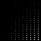
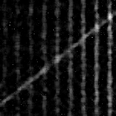
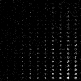
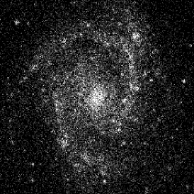
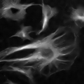
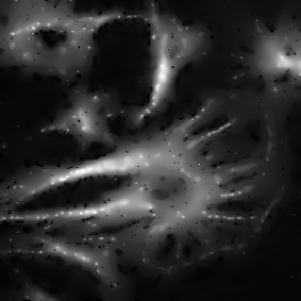
Refer to caption Refer to caption Refer to caption Refer to caption Refer to caption
NMISE=0.1009 NMISE=0.0593 NMISE=0.0368 NMISE=0.1150 NMISE=0.0870
M=19×19𝑀1919M=19\times 19 M=13×13𝑀1313M=13\times 13 M=9×9𝑀99M=9\times 9 M=15×15𝑀1515M=15\times 15 M=7×7𝑀77M=7\times 7
m=13×13𝑚1313m=13\times 13 m=3×3𝑚33m=3\times 3 m=21×21𝑚2121m=21\times 21 m=21×21𝑚2121m=21\times 21 m=13×13𝑚1313m=13\times 13
(a) Spots (b) Galaxy (c) Ridges (d) Barbara (e) Cells
Figure 1: These images restored by the first step of our algorithm.

4.2 Numerical performance of the Non-Local Means Poisson Filter

By simulations we found that the images with brightness between 00 and 255255255 (like Barbara) are well denoised by the first step, but for the low count levels images (with brightness less than μ𝜇\mu), the restored images by NLMPF are not smooth enough (see Figure 1). This explains why for the low count level images, we smooth the restored images by step 2.

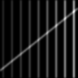
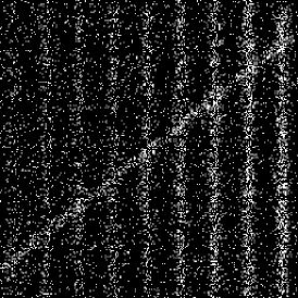
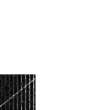
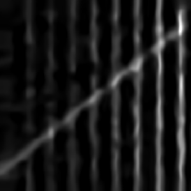
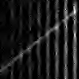
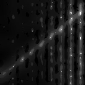
Our experiments are done in the same way as in ZHANG2008WAVELETS and MAKITALO2009INVERSION to produce comparable results; we also use the same set of test images (all of 256×256256256256\times 256 in size): Spots [0.08,4.99]0.084.99[0.08,4.99], Galaxy [0,5]05[0,5], Ridges [0.05,0.85]0.050.85[0.05,0.85], Barbara [0.93,15.73]0.9315.73[0.93,15.73], and Cells [0.53,16.93]0.5316.93[0.53,16.93]. The authors of ZHANG2008WAVELETS and MAKITALO2009INVERSION kindly provided us with their programs and the test images. A matlab implementation of the algorithms derived in this paper is available online111http://www.pami.sjtu.edu.cn/people/jinqy/. This unoptimized implemen-tation processes the set of 256×256256256256\times 256 test images 145145145 seconds with a search window of size 15×15151515\times 15 and patches of size 21×21212121\times 21, 525252 seconds with a search window of size 9×9999\times 9 and patches of size 21×21212121\times 21. The computational time is of about 10s per iteration on a 256×256256256256\times 256 image and Matlab on an Intel Pentium Dual CPU T3200 32-bit @ 2.00GHz CPU 3.00GHz.

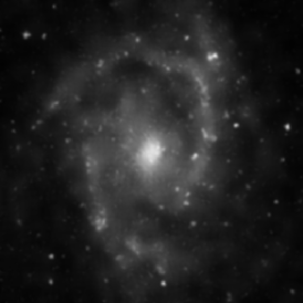
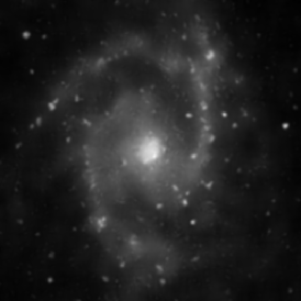
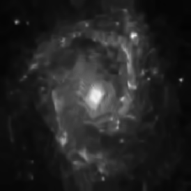
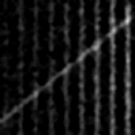
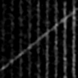
Table 1 shows the NMISE values of images reconstructed by NLMPF, OWPNF (jin2012new, ), Poisson NLM (deledalle2010poisson, ), EUI+BM3D makitalo2011optimal , MS-VST+7/9797/9 ZHANG2008WAVELETS and MS-VST+B3 ZHANG2008WAVELETS . Our algorithm reach the best in the case of Galaxy[0,5]05[0,5], while OWPNF reach the best in the case of Spots[0.08,4.99]0.084.99[0.08,4.99]; for Ridges[0.05,0.85]0.050.85[0.05,0.85], Barbara[0.93,15.73]0.9315.73[0.93,15.73], and Cells[0.53,16.93]0.5316.93[0.53,16.93], the method EUI+BM3D gives the best results, but our method is also very competitive. Table 2 shows the PSNR values of images reconstructed. Our algorithm also reach the best in the case of Galaxy[0,5]05[0,5]. The method EUI+BM3D have the highest PSNR value. However, the most important evaluation criteria is the visual quality of restored image. Figures 2- 6 illustrate the visual quality of these denoised images. It is obvious that The visual quality of the outputs of our method have high visual quality and many details Remained. For example, in the case of restored images of Spots (cf. Figures 2), our algorithm and OWPNF remain most spots. We can see clearly 777 spots at the third column (from left) in Figures 2 (c), while EUI+BM3D just remains 444 spots, Poisson NLM Makes several spots sticking together, the images restored by MS-VST + 7/9 and MS-VST + B3 are not smooth enough. In the case of Galaxy (cf. Figures 3), visually, our algorithm best preserves the fine textures. In the other case, our method also lead to good result visually.

Table 1: A comparison of the denoising performance (NMISE) of several denoising algorithms.
Algorithm Our OWPNF Poisson EUI+ MS-VST MS-VST
algorithm NLM BM3D +7/9797/9 +B3
Spots[0.08,4.99]0.084.99[0.08,4.99] 0.02600.0260{0.0260} 0.02590.0259\mathbf{0.0259} 0.0790 0.03580.03580.0358 0.06020.06020.0602 0.08100.08100.0810
Galaxy[0,5]05[0,5] 0.02840.0284\mathbf{0.0284} 0.02850.0285{0.0285} 0.0346 0.02970.02970.0297 0.03570.03570.0357 0.03380.03380.0338
Ridges[0.05,0.85]0.050.85[0.05,0.85] 0.01400.01400.0140 0.01620.01620.0162 0.0154 0.01210.0121\mathbf{0.0121} 0.01930.01930.0193 0.04160.04160.0416
Barbara[0.93,15.73]0.9315.73[0.93,15.73] 0.11500.11500.1150 0.10610.10610.1061 0.1207 0.08630.0863\mathbf{0.0863} 0.23910.23910.2391 0.37770.37770.3777
Cells[0.53,16.93]0.5316.93[0.53,16.93] 0.07850.07850.0785 0.07940.07940.0794 0.0816 0.06430.0643\mathbf{0.0643} 0.09090.09090.0909 0.14870.14870.1487
Table 2: A comparison of the denoising performance (PSNR, DB) of several denoising algorithms.
Algorithm Our OWPNF Poisson EUI+ MS-VST MS-VST
algorithm NLM BM3D +7/9797/9 +B3
Spots[0.08,4.99]0.084.99[0.08,4.99] 31.4531.4531.45 31.3131.3131.31 31.12 31.9531.95\mathbf{31.95} 31.6431.6431.64 30.3530.3530.35
Galaxy[0,5]05[0,5] 28.0928.09\mathbf{28.09} 27.8027.8027.80 27.77 28.0428.0428.04 27.5727.5727.57 27.9427.9427.94
Ridges[0.05,0.85]0.050.85[0.05,0.85] 24.6924.6924.69 23.9023.9023.90 24.94 25.8925.89\mathbf{25.89} 24.4924.4924.49 24.0324.0324.03
Barbara[0.93,15.73]0.9315.73[0.93,15.73] 24.7124.7124.71 24.6024.6024.60 24.72 25.9225.92\mathbf{25.92} 21.8121.8121.81 20.2220.2220.22
Cells[0.53,16.93]0.5316.93[0.53,16.93] 29.0829.0829.08 29.9129.9129.91 29.40 30.1830.18\mathbf{30.18} 28.8728.8728.87 26.6926.6926.69

5 Conclusion

In this paper, we have present a new image denoising algorithm to deal with the Poisson noise model, which is based on the idea of Non-Local Mean. The ”Oracle” estimator is obtained by minimized a very tight upper bound of the Mean Square Error with changing the size of search window. It help to establish a theorem to show that the Non-Local Means Filter can effectively deal with Poisson noise with some modification. As a result, we successfully construct the new algorithm called Non-Local Means Poisson Filter and demonstrate in statistic theory that the filter converges at the usual optimal rate. The filter is as simple as the classic Non-Local Means and the simulation results show that our filter is very competitive. The idea of how to construct an algorithm for Poisson noise model is creative. With our idea, many algorithms to Remove Gaussian Noise could deal with the Poisson noise with some modification.

6 Appendix: Proofs of the main results

6.1 Proof of Theorem 2.1

Denoting for brevity

I1=(x𝐔x0,hwh(x)ρf,x0(x))2=(xx0heρf,x02(x)H2(x0)ρf,x0(x)xx0heρf,x02(x)H2(x0))2,subscript𝐼1superscriptsubscript𝑥subscript𝐔subscript𝑥0subscriptsuperscript𝑤𝑥subscript𝜌𝑓subscript𝑥0𝑥2superscriptsubscriptsubscriptnorm𝑥subscript𝑥0superscript𝑒superscriptsubscript𝜌𝑓subscript𝑥02𝑥superscript𝐻2subscript𝑥0subscript𝜌𝑓subscript𝑥0𝑥subscriptsubscriptnorm𝑥subscript𝑥0superscript𝑒superscriptsubscript𝜌𝑓subscript𝑥02𝑥superscript𝐻2subscript𝑥02I_{1}=\left(\sum_{x\in\mathbf{U}_{x_{0},h}}w^{*}_{h}(x)\rho_{f,x_{0}}(x)\right)^{2}=\left(\frac{\displaystyle\sum_{\|x-x_{0}\|_{\infty}\leq h}e^{-\frac{\rho_{f,x_{0}}^{2}(x)}{H^{2}(x_{0})}}\rho_{f,x_{0}}(x)}{\displaystyle\sum_{\|x-x_{0}\|_{\infty}\leq h}e^{-\frac{\rho_{f,x_{0}}^{2}(x)}{H^{2}(x_{0})}}}\right)^{2}, (34)

and

I2=f(x0)x𝐔x0,h(wh(x))2=f(x0)xx0he2ρf,x02(x)H2(x0)(xx0heρf,x02(x)H2(x0))2,subscript𝐼2𝑓subscript𝑥0subscript𝑥subscript𝐔subscript𝑥0superscriptsubscriptsuperscript𝑤𝑥2𝑓subscript𝑥0subscriptsubscriptnorm𝑥subscript𝑥0superscript𝑒2superscriptsubscript𝜌𝑓subscript𝑥02𝑥superscript𝐻2subscript𝑥0superscriptsubscriptsubscriptnorm𝑥subscript𝑥0superscript𝑒superscriptsubscript𝜌𝑓subscript𝑥02𝑥superscript𝐻2subscript𝑥02I_{2}={f}(x_{0})\sum_{x\in\mathbf{U}_{x_{0},h}}\left(w^{*}_{h}(x)\right)^{2}=\frac{{f}(x_{0})\displaystyle\sum_{\|x-x_{0}\|_{\infty}\leq h}e^{-2\frac{\rho_{f,x_{0}}^{2}(x)}{H^{2}(x_{0})}}}{\left(\displaystyle\sum_{\|x-x_{0}\|_{\infty}\leq h}e^{-\frac{\rho_{f,x_{0}}^{2}(x)}{H^{2}(x_{0})}}\right)^{2}}, (35)

then we have

g(wh)=I1+I2.𝑔subscriptsuperscript𝑤subscript𝐼1subscript𝐼2g(w^{*}_{h})=I_{1}+I_{2}. (36)

The conditions (13) and γ>2Lhβ𝛾2𝐿superscript𝛽\gamma>\sqrt{2}Lh^{\beta} imply that for xUx0,h𝑥subscript𝑈subscript𝑥0x\in U_{x_{0},h}, we have

L2xx02βH2(x)L2h2βγ212.superscript𝐿2superscriptsubscriptnorm𝑥subscript𝑥02𝛽superscript𝐻2𝑥superscript𝐿2superscript2𝛽superscript𝛾212\frac{L^{2}\|x-x_{0}\|_{\infty}^{2\beta}}{H^{2}(x)}\leq\frac{L^{2}h^{2\beta}}{\gamma^{2}}\leq\frac{1}{2}. (37)

Noting that et2H2(x0)superscript𝑒superscript𝑡2superscript𝐻2subscript𝑥0e^{-\frac{t^{2}}{H^{2}(x_{0})}}, t[0,γ/2)𝑡0𝛾2t\in[0,\gamma/\sqrt{2}) is decreasing, and using one term Taylor expansion, the inequality (37) implies that

xx0heρf,x02(x)H2(x0)subscriptsubscriptnorm𝑥subscript𝑥0superscript𝑒superscriptsubscript𝜌𝑓subscript𝑥02𝑥superscript𝐻2subscript𝑥0\displaystyle\displaystyle\sum_{\|x-x_{0}\|_{\infty}\leq h}e^{-\frac{\rho_{f,x_{0}}^{2}(x)}{H^{2}(x_{0})}} \displaystyle\geq xx0heL2xx02βH2(x0)xx0h(1L2xx02βH2(x0))subscriptsubscriptnorm𝑥subscript𝑥0superscript𝑒superscript𝐿2superscriptsubscriptnorm𝑥subscript𝑥02𝛽superscript𝐻2subscript𝑥0subscriptsubscriptnorm𝑥subscript𝑥01superscript𝐿2superscriptsubscriptnorm𝑥subscript𝑥02𝛽superscript𝐻2subscript𝑥0\displaystyle\sum_{\|x-x_{0}\|_{\infty}\leq h}e^{-\frac{L^{2}\|x-x_{0}\|_{\infty}^{2\beta}}{H^{2}(x_{0})}}\geq\sum_{\|x-x_{0}\|_{\infty}\leq h}\left(1-\frac{L^{2}\|x-x_{0}\|_{\infty}^{2\beta}}{H^{2}(x_{0})}\right) (38)
\displaystyle\geq 2h2n.2superscript2𝑛\displaystyle 2h^{2}n.

Considering that tet2H2(x0)𝑡superscript𝑒superscript𝑡2superscript𝐻2subscript𝑥0te^{-\frac{t^{2}}{H^{2}(x_{0})}}, t[0,γ/2)𝑡0𝛾2t\in[0,\gamma/\sqrt{2}) is increasing function,

xx0heρf,x02(x)H2(x0)ρf,x0(x)subscriptsubscriptnorm𝑥subscript𝑥0superscript𝑒superscriptsubscript𝜌𝑓subscript𝑥02𝑥superscript𝐻2subscript𝑥0subscript𝜌𝑓subscript𝑥0𝑥\displaystyle\sum_{\|x-x_{0}\|_{\infty}\leq h}e^{-\frac{\rho_{f,x_{0}}^{2}(x)}{H^{2}(x_{0})}}\rho_{f,x_{0}}(x) \displaystyle\leq xx0hLxx0βeL2xx02βH2(x0)subscriptsubscriptnorm𝑥subscript𝑥0𝐿subscriptsuperscriptnorm𝑥subscript𝑥0𝛽superscript𝑒superscript𝐿2superscriptsubscriptnorm𝑥subscript𝑥02𝛽superscript𝐻2subscript𝑥0\displaystyle\sum_{\|x-x_{0}\|_{\infty}\leq h}L\|x-x_{0}\|^{\beta}_{\infty}e^{-\frac{L^{2}\|x-x_{0}\|_{\infty}^{2\beta}}{H^{2}(x_{0})}} (39)
\displaystyle\leq xx0hLxx0β4Lhβ+2n.subscriptsubscriptnorm𝑥subscript𝑥0𝐿subscriptsuperscriptnorm𝑥subscript𝑥0𝛽4𝐿superscript𝛽2𝑛\displaystyle\sum_{\|x-x_{0}\|_{\infty}\leq h}L\|x-x_{0}\|^{\beta}_{\infty}\leq 4Lh^{\beta+2}n.

The above three inequalities (34), (38) and (39) imply that

I14L2h2β.subscript𝐼14superscript𝐿2superscript2𝛽I_{1}\leq 4L^{2}h^{2\beta}. (40)

Taking into account the inequality

xx0he2ρf,x02(x)H2(x0)xx0h1=4h2n,subscriptsubscriptnorm𝑥subscript𝑥0superscript𝑒2superscriptsubscript𝜌𝑓subscript𝑥02𝑥superscript𝐻2subscript𝑥0subscriptsubscriptnorm𝑥subscript𝑥014superscript2𝑛\sum_{\|x-x_{0}\|_{\infty}\leq h}e^{-2\frac{\rho_{f,x_{0}}^{2}(x)}{H^{2}(x_{0})}}\leq\sum_{\|x-x_{0}\|_{\infty}\leq h}1=4h^{2}n,

(35) and (38), it is easily seen that

I2Γh2n.subscript𝐼2Γsuperscript2𝑛I_{2}\leq\frac{\Gamma}{h^{2}n}. (41)

Combining (36), (40), and (41), we give

g(wh)4L2h2β+Γh2n.𝑔superscriptsubscript𝑤4superscript𝐿2superscript2𝛽Γsuperscript2𝑛g(w_{h}^{*})\leq 4L^{2}h^{2\beta}+\frac{\Gamma}{h^{2}n}. (42)

Let hh minimize the latter term of the above inequality (42). Then

8βL2h2β12Γh3n=08𝛽superscript𝐿2superscript2𝛽12Γsuperscript3𝑛08\beta L^{2}h^{2\beta-1}-\frac{2\Gamma}{h^{3}n}=0

from which we infer that

h=(Γ4βL2)12β+2n12β+2.superscriptΓ4𝛽superscript𝐿212𝛽2superscript𝑛12𝛽2h=\left(\frac{\Gamma}{4\beta L^{2}}\right)^{\frac{1}{2\beta+2}}n^{-\frac{1}{2\beta+2}}. (43)

Substituting (43) to (42) leads to

g(wh)22β+62β+2Γ2β2β+2L42β+2β2β2β+2n2β2β+2.𝑔superscriptsubscript𝑤superscript22𝛽62𝛽2superscriptΓ2𝛽2𝛽2superscript𝐿42𝛽2superscript𝛽2𝛽2𝛽2superscript𝑛2𝛽2𝛽2g(w_{h}^{*})\leq\frac{2^{\frac{2\beta+6}{2\beta+2}}\Gamma^{\frac{2\beta}{2\beta+2}}L^{\frac{4}{2\beta+2}}}{\beta^{\frac{2\beta}{2\beta+2}}}n^{-\frac{2\beta}{2\beta+2}}.

Therefore (47) implies (19).

6.2 Proof of Theorem 3.1

We shall use following lemma to finish the Proof of Theorem 3.1. The lemma can be deduced form the results in Borovkov borovkov2000estimates , see also Merlevede, Peligrad and Rio merleve2010bernstein

Lemma 1

If, for some δ>0,γ(0,1)formulae-sequence𝛿0𝛾01\delta>0,\gamma\in(0,1) and K>1𝐾1K>1 we have

sup𝔼exp(δ|Xi|γ)K,i=1,,n,formulae-sequencesupremum𝔼𝛿superscriptsubscript𝑋𝑖𝛾𝐾𝑖1𝑛\sup\mathbb{E}\exp\left(\delta\left|X_{i}\right|^{\gamma}\right)\leq K,\;i=1,...,n,

then there are two positive constants c1subscript𝑐1c_{1} and c2subscript𝑐2c_{2} depending only on δ,𝛿\delta, γ𝛾\gamma and K𝐾K such that, for any t>0,𝑡0t>0,

(i=1nXit)exp(c1t2/n)+nexp(c2tγ).superscriptsubscript𝑖1𝑛subscript𝑋𝑖𝑡subscript𝑐1superscript𝑡2𝑛𝑛subscript𝑐2superscript𝑡𝛾\mathbb{P}\left(\sum_{i=1}^{n}X_{i}\geq t\right)\leq\exp\left(-c_{1}t^{2}/n\right)+n\exp\left(-c_{2}t^{\gamma}\right).

Proof of Theorem 3.1. Recall that M𝑀M and m𝑚m is given by (5) and (6) respectively. Consider that

|ρ^x02(x)ρf,x02(x)||1mS(x)+1mR(x)|,superscriptsubscript^𝜌subscript𝑥02𝑥superscriptsubscript𝜌𝑓subscript𝑥02𝑥1𝑚𝑆𝑥1𝑚𝑅𝑥|\widehat{\rho}_{x_{0}}^{2}(x)-\rho_{f,x_{0}}^{2}(x)|\leq\left|\frac{1}{m}S(x)+\frac{1}{m}R(x)\right|, (44)

where

S(x)=y𝐔x0,ηZ(y),𝑆𝑥subscript𝑦subscript𝐔subscript𝑥0𝜂𝑍𝑦S(x)=\sum_{y\in\mathbf{U}_{x_{0},\eta}}Z(y),
Z(y)=(Y(y)Y(Txy))2(f(y)f(Txy))2f(y)f(Txy),𝑍𝑦superscript𝑌𝑦𝑌subscript𝑇𝑥𝑦2superscript𝑓𝑦𝑓subscript𝑇𝑥𝑦2𝑓𝑦𝑓subscript𝑇𝑥𝑦Z(y)=(Y(y)-Y(T_{x}y))^{2}-(f(y)-f(T_{x}y))^{2}-f(y)-f(T_{x}y), (45)

and

R(x)=y𝐔x0,η((f(y)f(Txy))2+f(y)+f(Txy))(f(x0)f(x))22f¯(x0).𝑅𝑥subscript𝑦subscript𝐔subscript𝑥0𝜂superscript𝑓𝑦𝑓subscript𝑇𝑥𝑦2𝑓𝑦𝑓subscript𝑇𝑥𝑦superscript𝑓subscript𝑥0𝑓𝑥22¯𝑓subscript𝑥0R(x)=\sum_{y\in\mathbf{U}_{x_{0},\eta}}\left((f(y)-f(T_{x}y))^{2}+f(y)+f(T_{x}y)\right)-(f(x_{0})-f(x))^{2}-2\overline{f}(x_{0}).

Since Y(x)𝑌𝑥Y(x) has the Poisson distribution, with mean f(x)𝑓𝑥f(x) and variance f(x)𝑓𝑥f(x),

𝔼(eY(x))=k=0+ekfk(x)ef(x)k!=ef(x)e(e1)f(x)eΓe(e1)Γ.𝔼superscript𝑒𝑌𝑥superscriptsubscript𝑘0superscript𝑒𝑘superscript𝑓𝑘𝑥superscript𝑒𝑓𝑥𝑘𝑒𝑓𝑥superscript𝑒𝑒1𝑓𝑥𝑒Γsuperscript𝑒𝑒1Γ\mathbb{E}\left(e^{Y(x)}\right)=\sum_{k=0}^{+\infty}e^{k}\frac{f^{k}(x)e^{-f(x)}}{k!}=ef(x)e^{(e-1)f(x)}\leq e\Gamma e^{(e-1)\Gamma}. (46)

From the inequality (46), we easily deduce

sup𝔼(e|Z(y)|1/2)sup𝔼(eY(y)+Y(Txy)+2Γ+2Γ)(eΓ)2e2eΓ+2Γsupremum𝔼superscript𝑒superscript𝑍𝑦12supremum𝔼superscript𝑒𝑌𝑦𝑌subscript𝑇𝑥𝑦2Γ2Γsuperscript𝑒Γ2superscript𝑒2𝑒Γ2Γ\sup\mathbb{E}\left(e^{|Z(y)|^{1/2}}\right)\leq\sup\mathbb{E}\left(e^{Y(y)+Y(T_{x}y)+2\Gamma+2\sqrt{\Gamma}}\right)\leq(e\Gamma)^{2}e^{2e\Gamma+2\sqrt{\Gamma}} (47)

By Lemma 1, we see that there are two positive constants c5subscript𝑐5c_{5} and c6subscript𝑐6c_{6} such that for any z>0𝑧0z>0,

(1m|S(x)|zm)exp(c5z2)+mexp(c6(mz)12).1𝑚𝑆𝑥𝑧𝑚subscript𝑐5superscript𝑧2𝑚subscript𝑐6superscript𝑚𝑧12\mathbb{P}\left(\frac{1}{m}|S(x)|\geq\frac{z}{\sqrt{m}}\right)\leq\exp(-c_{5}z^{2})+m\exp(-c_{6}(\sqrt{m}z)^{\frac{1}{2}}). (48)

Considering m=(2Nη+1)2𝑚superscript2𝑁𝜂12m=(2N\eta+1)^{2} and η=c1nα((1β)+)2β+2<α<12\eta=c_{1}n^{-\alpha}(\frac{(1-\beta)^{+})}{2\beta+2}<\alpha<\frac{1}{2}, we have m=c1n12α(1+o(1))𝑚subscriptsuperscript𝑐1superscript𝑛12𝛼1𝑜1m=c^{\prime}_{1}n^{1-2\alpha}(1+o(1)). Therefore, substituting z=1c5lnn2𝑧1subscript𝑐5superscript𝑛2z=\sqrt{\frac{1}{c_{5}}\ln n^{2}} into the inequality (48), we see that for n𝑛n large enough,

(1m|S(x)|1c5lnn2m)2exp(lnn2)=2n2.1𝑚𝑆𝑥1subscript𝑐5superscript𝑛2𝑚2superscript𝑛22superscript𝑛2\mathbb{P}\left(\frac{1}{m}\left|S(x)\right|\geq\frac{\sqrt{\frac{1}{c_{5}}\ln n^{2}}}{\sqrt{m}}\right)\leq 2\exp\left(-\ln n^{2}\right)=\frac{2}{n^{2}}.

From this inequality we easily deduce that

(maxx𝐔x0,h1m|S(x)|1c5lnn2m)x𝐔x0,h(1m|S(x)|1c5lnn2m)2n.subscript𝑥subscript𝐔subscript𝑥01𝑚𝑆𝑥1subscript𝑐5superscript𝑛2𝑚subscript𝑥subscript𝐔subscript𝑥01𝑚𝑆𝑥1subscript𝑐5superscript𝑛2𝑚2𝑛\mathbb{P}\left(\max_{x\in\mathbf{U}_{x_{0},h}}\frac{1}{m}\left|S(x)\right|\geq\frac{\sqrt{\frac{1}{c_{5}}\ln n^{2}}}{\sqrt{m}}\right)\leq\sum_{x\in\mathbf{U}_{x_{0},h}}\mathbb{P}\left(\frac{1}{m}\left|S(x)\right|\geq\frac{\sqrt{\frac{1}{c_{5}}\ln n^{2}}}{\sqrt{m}}\right)\leq\frac{2}{n}.

We arrive at

(𝐁)c7n1,𝐁subscript𝑐7superscript𝑛1\mathbb{P}\left(\mathbf{B}\right)\leq c_{7}n^{-1}, (49)

where 𝐁={maxx𝐔x0,h1m|S(x)|<c8nα12lnn}𝐁subscript𝑥subscript𝐔subscript𝑥01𝑚𝑆𝑥subscript𝑐8superscript𝑛𝛼12𝑛\mathbf{B}=\{\max_{x\in\mathbf{U}_{x_{0},h}}\frac{1}{m}\left|S(x)\right|<c_{8}n^{\alpha-\frac{1}{2}}\sqrt{\ln n}\} and c8subscript𝑐8c_{8} is a constant depending only on β𝛽\beta and L𝐿L. It is easy to see that

R(x)=O(nα12).𝑅𝑥𝑂superscript𝑛𝛼12R(x)=O\left(n^{\alpha-\frac{1}{2}}\right). (50)

In the set 𝐁𝐁\mathbf{B}, the inequality (50) implies that

maxx𝐔x0,h|ρ^x02(x)ρf,x02(x)|c8nβ2β+2lnn+O(nα12)=O(nβ2β+2lnn).subscript𝑥subscript𝐔subscript𝑥0superscriptsubscript^𝜌subscript𝑥02𝑥superscriptsubscript𝜌𝑓subscript𝑥02𝑥subscript𝑐8superscript𝑛𝛽2𝛽2𝑛𝑂superscript𝑛𝛼12𝑂superscript𝑛𝛽2𝛽2𝑛\max_{x\in\mathbf{U}_{x_{0},h}}|\widehat{\rho}_{x_{0}}^{2}(x)-\rho_{f,x_{0}}^{2}(x)|\leq c_{8}n^{-\frac{\beta}{2\beta+2}}\sqrt{\ln n}+O\left(n^{\alpha-\frac{1}{2}}\right)=O(n^{-\frac{\beta}{2\beta+2}}\sqrt{\ln n}). (51)

Combining (49) and (51), we obtain (22).

6.3 Proof of Theorem 3.2

Taking into account (25), (27), and the independence of ϵ(x)italic-ϵ𝑥\epsilon(x), we have

𝔼{|f^h(x0)f(x0)|2|Y(x),x𝐈x0′′}g(w^h),𝔼conditionalsuperscriptsubscriptsuperscript^𝑓subscript𝑥0𝑓subscript𝑥02𝑌𝑥𝑥subscriptsuperscript𝐈′′subscript𝑥0superscript𝑔subscript^𝑤\mathbb{E}\{|\widehat{f}^{\prime}_{h}(x_{0})-f(x_{0})|^{2}\big{|}Y(x),x\in\mathbf{I}^{\prime\prime}_{x_{0}}\}\leq g^{\prime}(\widehat{w}_{h}), (52)

where

g(w)=(x𝐔x0,hw(x)ρf,x0(x))2+f¯(x0)x𝐈x0w2(x).superscript𝑔𝑤superscriptsubscript𝑥subscriptsuperscript𝐔subscript𝑥0𝑤𝑥subscript𝜌𝑓subscript𝑥0𝑥2superscript¯𝑓subscript𝑥0subscript𝑥subscriptsuperscript𝐈subscript𝑥0superscript𝑤2𝑥g^{\prime}(w)=\left(\sum_{x\in\mathbf{U}^{\prime}_{x_{0},h}}{w}(x)\rho_{f,x_{0}}(x)\right)^{2}+\overline{f}^{\prime}(x_{0})\sum_{x\in\mathbf{I}^{\prime}_{x_{0}}}{w}^{2}(x).

By the proof of Theorem 2.1, we obtain

g(wh)32(22β+62β+2Γ2β2β+2L42β+2β2β2β+2n2β2β+2).superscript𝑔subscriptsuperscript𝑤32superscript22𝛽62𝛽2superscriptΓ2𝛽2𝛽2superscript𝐿42𝛽2superscript𝛽2𝛽2𝛽2superscript𝑛2𝛽2𝛽2g^{\prime}(w^{\ast}_{h})\leq\frac{3}{2}\left(\frac{2^{\frac{2\beta+6}{2\beta+2}}\Gamma^{\frac{2\beta}{2\beta+2}}L^{\frac{4}{2\beta+2}}}{\beta^{\frac{2\beta}{2\beta+2}}}n^{-\frac{2\beta}{2\beta+2}}\right). (53)

By Theorem 3.1 and its proof, for ρ^x0subscriptsuperscript^𝜌subscript𝑥0\widehat{\rho}^{\prime}_{x_{0}} is defined by (25), there is a constant c2subscript𝑐2c_{2} such that

{maxx𝐔x0,h|ρ^x02(x)ρf,x02(x)|c2nα12lnn}=O(n1).\mathbb{P}\left\{\max_{x\in\mathbf{U}^{\prime}_{x_{0},h}}\left|\widehat{\rho}_{x_{0}}^{{}^{\prime}2}(x)-\rho_{f,x_{0}}^{2}(x)\right|\geq c_{2}n^{\alpha-\frac{1}{2}}\sqrt{\ln n}\right\}=O\left(n^{-1}\right). (54)

Let 𝐁={maxx𝐔x0,h|ρ^x02(x)ρf,x02(x)|c2nα12lnn}\mathbf{B}=\left\{\max_{x\in\mathbf{U}^{\prime}_{x_{0},h}}\left|\widehat{\rho}_{x_{0}}^{{}^{\prime}2}(x)-\rho_{f,x_{0}}^{2}(x)\right|\leq c_{2}n^{\alpha-\frac{1}{2}}\ln n\right\}. On the set 𝐁𝐁\mathbf{B}, we have ρf,x02(x)c2nα12lnn<ρ^x02(x)<ρf,x02(x)+c2nα12lnn\rho_{f,x_{0}}^{2}(x)-c_{2}n^{\alpha-\frac{1}{2}}\sqrt{\ln n}<\widehat{\rho}_{x_{0}}^{{}^{\prime}2}(x)<\rho_{f,x_{0}}^{2}(x)+c_{2}n^{\alpha-\frac{1}{2}}\sqrt{\ln n}, from which we infer that

w^(x)^𝑤𝑥\displaystyle\widehat{w}(x) =\displaystyle= eρ^x02(x)H2(x0)x𝐔x0,heρ^x02(x)H2(x0)eρf,x02(x)c2nα12lnnH2(x0)x𝐔x0,heρf,x02(x)+c2nα12lnnH2(x0)\displaystyle\frac{e^{-\frac{\widehat{\rho}_{x_{0}}^{{}^{\prime}2}(x)}{H^{2}(x_{0})}}}{\sum_{x^{\prime}\in\mathbf{U}_{x_{0},h}^{\prime}}e^{-\frac{\widehat{\rho}_{x_{0}}^{{}^{\prime}2}(x^{\prime})}{H^{2}(x_{0})}}}\leq\frac{e^{-\frac{{\rho}_{f,x_{0}}^{2}(x)-c_{2}n^{\alpha-\frac{1}{2}}\sqrt{\ln n}}{H^{2}(x_{0})}}}{\sum_{x^{\prime}\in\mathbf{U}_{x_{0},h}^{\prime}}e^{-\frac{{\rho}_{f,x_{0}}^{2}(x^{\prime})+c_{2}n^{\alpha-\frac{1}{2}}\sqrt{\ln n}}{H^{2}(x_{0})}}}
\displaystyle\leq eρf,x02(x)H2(x0)(1+2c2nα12lnnH2(x0))x𝐔x0,heρf,x02(x)H2(x0)(1c2nα12lnnH2(x0))superscript𝑒superscriptsubscript𝜌𝑓subscript𝑥02𝑥superscript𝐻2subscript𝑥012subscript𝑐2superscript𝑛𝛼12𝑛superscript𝐻2subscript𝑥0subscriptsuperscript𝑥superscriptsubscript𝐔subscript𝑥0superscript𝑒superscriptsubscript𝜌𝑓subscript𝑥02superscript𝑥superscript𝐻2subscript𝑥01subscript𝑐2superscript𝑛𝛼12𝑛superscript𝐻2subscript𝑥0\displaystyle\frac{e^{-\frac{{\rho}_{f,x_{0}}^{2}(x)}{H^{2}(x_{0})}}\left(1+2\frac{c_{2}n^{\alpha-\frac{1}{2}}\sqrt{\ln n}}{H^{2}(x_{0})}\right)}{\sum_{x^{\prime}\in\mathbf{U}_{x_{0},h}^{\prime}}e^{-\frac{{\rho}_{f,x_{0}}^{2}(x^{\prime})}{H^{2}(x_{0})}}\left(1-\frac{c_{2}n^{\alpha-\frac{1}{2}}\sqrt{\ln n}}{H^{2}(x_{0})}\right)}
=\displaystyle= (1+2c2nα12lnnH2(x0)1c2nα12lnnH2(x0))eρf,x02(x)H2(x0)x𝐔x0,heρf,x02(x)H2(x0)12subscript𝑐2superscript𝑛𝛼12𝑛superscript𝐻2subscript𝑥01subscript𝑐2superscript𝑛𝛼12𝑛superscript𝐻2subscript𝑥0superscript𝑒superscriptsubscript𝜌𝑓subscript𝑥02𝑥superscript𝐻2subscript𝑥0subscriptsuperscript𝑥superscriptsubscript𝐔subscript𝑥0superscript𝑒superscriptsubscript𝜌𝑓subscript𝑥02superscript𝑥superscript𝐻2subscript𝑥0\displaystyle\left(\frac{1+\frac{2c_{2}n^{\alpha-\frac{1}{2}}\sqrt{\ln n}}{H^{2}(x_{0})}}{1-\frac{c_{2}n^{\alpha-\frac{1}{2}}\sqrt{\ln n}}{H^{2}(x_{0})}}\right)\frac{e^{-\frac{{\rho}_{f,x_{0}}^{2}(x)}{H^{2}(x_{0})}}}{\sum_{x^{\prime}\in\mathbf{U}_{x_{0},h}^{\prime}}e^{-\frac{{\rho}_{f,x_{0}}^{2}(x^{\prime})}{H^{2}(x_{0})}}}
=\displaystyle= (1+2c2nα12lnnH2(x0)1c2nα12lnnH2(x0))wh(x).12subscript𝑐2superscript𝑛𝛼12𝑛superscript𝐻2subscript𝑥01subscript𝑐2superscript𝑛𝛼12𝑛superscript𝐻2subscript𝑥0subscriptsuperscript𝑤𝑥\displaystyle\left(\frac{1+\frac{2c_{2}n^{\alpha-\frac{1}{2}}\sqrt{\ln n}}{H^{2}(x_{0})}}{1-\frac{c_{2}n^{\alpha-\frac{1}{2}}\sqrt{\ln n}}{H^{2}(x_{0})}}\right)w^{*}_{h}(x).

This implies that

g(w^h)(1+2c2nα12lnnH2(x0)1c2nα12lnnH2(x0))2g(wh).superscript𝑔subscript^𝑤superscript12subscript𝑐2superscript𝑛𝛼12𝑛superscript𝐻2subscript𝑥01subscript𝑐2superscript𝑛𝛼12𝑛superscript𝐻2subscript𝑥02superscript𝑔subscriptsuperscript𝑤g^{\prime}(\widehat{w}_{h})\leq\left(\frac{1+\frac{2c_{2}n^{\alpha-\frac{1}{2}}\sqrt{\ln n}}{H^{2}(x_{0})}}{1-\frac{c_{2}n^{\alpha-\frac{1}{2}}\sqrt{\ln n}}{H^{2}(x_{0})}}\right)^{2}g^{\prime}(w^{*}_{h}).

The condition 4c2nα12lnn<γH2(x0)4subscript𝑐2superscript𝑛𝛼12𝑛𝛾superscript𝐻2subscript𝑥04c_{2}n^{\alpha-\frac{1}{2}}\sqrt{\ln n}<\gamma\leq H^{2}(x_{0}) implies that

(1+2c2nα12lnnH2(x0)1c2nα12lnnH2(x0))22.superscript12subscript𝑐2superscript𝑛𝛼12𝑛superscript𝐻2subscript𝑥01subscript𝑐2superscript𝑛𝛼12𝑛superscript𝐻2subscript𝑥022\left(\frac{1+\frac{2c_{2}n^{\alpha-\frac{1}{2}}\sqrt{\ln n}}{H^{2}(x_{0})}}{1-\frac{c_{2}n^{\alpha-\frac{1}{2}}\sqrt{\ln n}}{H^{2}(x_{0})}}\right)^{2}\leq 2.

Consequently, (52) becomes

𝔼(|f^h(x0)f(x0)|2|Y(x),x𝐈x0′′,𝐁)2g(wh).𝔼conditionalsuperscriptsubscriptsuperscript^𝑓subscript𝑥0𝑓subscript𝑥02𝑌𝑥𝑥subscriptsuperscript𝐈′′subscript𝑥0𝐁2superscript𝑔subscriptsuperscript𝑤\mathbb{E}\left(|\widehat{f}^{\prime}_{h}(x_{0})-f(x_{0})|^{2}\big{|}Y(x),x\in\mathbf{I}^{\prime\prime}_{x_{0}},\mathbf{B}\right)\leq 2g^{\prime}(w^{*}_{h}). (55)

Since the function f𝑓f satisfies the Hölder condition,

𝔼(|f^h(x0)f(x0)|2|Y(x),x𝐈x0′′)<g(w^h)c9,𝔼conditionalsuperscriptsubscriptsuperscript^𝑓subscript𝑥0𝑓subscript𝑥02𝑌𝑥𝑥subscriptsuperscript𝐈′′subscript𝑥0superscript𝑔subscript^𝑤subscript𝑐9\mathbb{E}\left(|\widehat{f}^{\prime}_{h}(x_{0})-f(x_{0})|^{2}\big{|}Y(x),x\in\mathbf{I}^{\prime\prime}_{x_{0}}\right)<g^{\prime}(\widehat{w}_{h})\leq c_{9}, (56)

for a constant c9>0subscript𝑐90c_{9}>0 depending only on β𝛽\beta and L𝐿L. Combining (22), (55), and (56), we have

𝔼𝔼\displaystyle\mathbb{E} (|f^h(x0)f(x0)|2|Y(x),x𝐈x0′′)conditionalsuperscriptsubscriptsuperscript^𝑓subscript𝑥0𝑓subscript𝑥02𝑌𝑥𝑥subscriptsuperscript𝐈′′subscript𝑥0\displaystyle\left(|\widehat{f}^{\prime}_{h}(x_{0})-f(x_{0})|^{2}\big{|}Y(x),x\in\mathbf{I}^{\prime\prime}_{x_{0}}\right)
=\displaystyle= 𝔼(|f^h(x0)f(x0)|2|Y(x),x𝐈x0′′,𝐁)(𝐁)𝔼conditionalsuperscriptsubscriptsuperscript^𝑓subscript𝑥0𝑓subscript𝑥02𝑌𝑥𝑥subscriptsuperscript𝐈′′subscript𝑥0𝐁𝐁\displaystyle\mathbb{E}\left(|\widehat{f}^{\prime}_{h}(x_{0})-f(x_{0})|^{2}\big{|}Y(x),x\in\mathbf{I}^{\prime\prime}_{x_{0}},\mathbf{B}\right)\mathbb{P}(\mathbf{B})
+𝔼(|f^h(x0)f(x0)|2|Y(x),x𝐈x0′′,𝐁¯)(𝐁¯)𝔼conditionalsuperscriptsubscriptsuperscript^𝑓subscript𝑥0𝑓subscript𝑥02𝑌𝑥𝑥subscriptsuperscript𝐈′′subscript𝑥0¯𝐁¯𝐁\displaystyle+\mathbb{E}\left(|\widehat{f}^{\prime}_{h}(x_{0})-f(x_{0})|^{2}\big{|}Y(x),x\in\mathbf{I}^{\prime\prime}_{x_{0}},\overline{\mathbf{B}}\right)\mathbb{P}(\overline{\mathbf{B}})
\displaystyle\leq 2g(wh)+O(n1)2superscript𝑔subscriptsuperscript𝑤𝑂superscript𝑛1\displaystyle 2g^{\prime}(w^{*}_{h})+O\left(n^{-1}\right)

Now, the assertion of the theorem is obtained easily if we take into account (53).

References

  • (1) I. Abraham, R. Abraham, A. Desolneux, and S. Li-Thiao-Te. Significant edges in the case of non-stationary gaussian noise. Pattern recognition, 40(11):3277–3291, 2007.
  • (2) M. Aharon, M. Elad, and A. Bruckstein. rmk𝑟𝑚𝑘rmk-svd: An algorithm for designing overcomplete dictionaries for sparse representation. IEEE Trans. Signal Process., 54(11):4311–4322, 2006.
  • (3) F. Alter, Y. Matsushita, and X. Tang. An intensity similarity measure in low-light conditions. Computer Vision–ECCV 2006, pages 267–280, 2006.
  • (4) F.J. Anscombe. The transformation of poisson, binomial and negative-binomial data. Biometrika, 35(3/4):246–254, 1948.
  • (5) A. Beck and M. Teboulle. Fast gradient-based algorithms for constrained total variation image denoising and deblurring problems. IEEE Trans. Image Process., 18(11):2419–2434, 2009.
  • (6) A.A. Borovkov. Estimates for the distribution of sums and maxima of sums of random variables without the cramer condition. Siberian Mathematical Journal, 41(5):811–848, 2000.
  • (7) J. Boulanger, J.B. Sibarita, C. Kervrann, and P. Bouthemy. Non-parametric regression for patch-based fluorescence microscopy image sequence denoising. In in Proc. of IEEE Int. Symp. on Biomedical Imaging: From Nano to Macro, ISBI 2008, pages 748–751. IEEE, 2008.
  • (8) A. Buades, B. Coll, and J.M. Morel. A review of image denoising algorithms, with a new one. SIAM Journal on Multiscale Modeling and Simulation, 4(2):490–530, 2005.
  • (9) T. Buades, Y. Lou, JM Morel, and Z. Tang. A note on multi-image denoising. In Int. workshop on Local and Non-Local Approximation in Image Processing, pages 1–15, August 2009.
  • (10) C.A. Deledalle, F. Tupin, and L. Denis. Poisson nl means: Unsupervised non local means for poisson noise. In IEEE Int. Conf. on Image Process. (ICIP), 2010 17th, pages 801–804. IEEE, 2010.
  • (11) D.L. Donoho and J.M. Johnstone. Ideal spatial adaptation by wavelet shrinkage. Biometrika, 81(3):425, 1994.
  • (12) J. Fan. Local linear regression smoothers and their minimax efficiencies. The Annals of Statistics, pages 196–216, 1993.
  • (13) J.Q. Fan and I. Gijbels. Local polynomial modelling and its applications. In Chapman & Hall, London, 1996.
  • (14) P. Fryzlewicz, V. Delouille, and G.P. Nason. Goes-8 x-ray sensor variance stabilization using the multiscale data-driven haar–fisz transform. J. Roy. Statist. Soc. ser. C, 56(1):99–116, 2007.
  • (15) P. Fryzlewicz and G.P. Nason. A haar-fisz algorithm for poisson intensity estimation. J. Comp. Graph. Stat., 13(3):621–638, 2004.
  • (16) D.K. Hammond and E.P. Simoncelli. Image modeling and denoising with orientation-adapted gaussian scale mixtures. IEEE Trans. Image Process., 17(11):2089–2101, 2008.
  • (17) K. Hirakawa and T.W. Parks. Image denoising using total least squares. IEEE Trans. Image Process., 15(9):2730–2742, 2006.
  • (18) M. Jansen. Multiscale poisson data smoothing. J. Roy. Statist. Soc. B, 68(1):27–48, 2006.
  • (19) Qiyu Jin, Ion Grama, and Quansheng Liu. A new poisson noise filter based on weights optimization. arXiv preprint arXiv:1201.5968, 2012.
  • (20) Q.Y. Jin, I. Grama, and Q.S. Liu. Removing gaussian noise by optimization of weights in non-local means. http://arxiv.org/abs/1109.5640.
  • (21) V. Katkovnik, A. Foi, K. Egiazarian, and J. Astola. From local kernel to nonlocal multiple-model image denoising. Int. J. Comput. Vis., 86(1):1–32, 2010.
  • (22) C. Kervrann and J. Boulanger. Optimal spatial adaptation for patch-based image denoising. IEEE Trans. Image Process., 15(10):2866–2878, 2006.
  • (23) E.D. Kolaczyk and R.D. Nowak. Multiscale generalised linear models for nonparametric function estimation. Biometrika, 92(1):119, 2005.
  • (24) T. Le, R. Chartrand, and T. J. Asaki. A variational approach to reconstructing images corrupted by poisson noise. Journal of Mathematical Imaging and Vision, 27(3):257–263, 2007.
  • (25) S. Lefkimmiatis, P. Maragos, and G. Papandreou. Bayesian inference on multiscale models for poisson intensity estimation: Applications to photon-limited image denoising. IEEE Trans. Image Process., 18(8):1724–1741, 2009.
  • (26) F. Luisier, C. Vonesch, T. Blu, and M. Unser. Fast interscale wavelet denoising of poisson-corrupted images. Signal Process., 90(2):415–427, 2010.
  • (27) J. Mairal, G. Sapiro, and M. Elad. Learning multiscale sparse representations for image and video restoration. SIAM Multiscale Modeling and Simulation, 7(1):214–241, 2008.
  • (28) M. Makitalo and A. Foi. On the inversion of the anscombe transformation in low-count poisson image denoising. In Proc. Int. Workshop on Local and Non-Local Approx. in Image Process., LNLA 2009, Tuusula, Finland, pages 26–32. IEEE, 2009.
  • (29) M. Makitalo and A. Foi. Optimal inversion of the anscombe transformation in low-count poisson image denoising. IEEE Trans. Image Process., 20(1):99–109, 2011.
  • (30) J. Mandel. Use of the singular value decomposition in regression analysis. The American Statistician, 36(1):15–24, 1982.
  • (31) F. Merlevède, M. Peligrad, and E. Rio. A bernstein type inequality and moderate deviations for weakly dependent sequences. Probab. Theory Related Fields, 2010.
  • (32) I. Moon and B. Javidi. Three dimensional imaging and recognition using truncated photon counting model and parametric maximum likelihood estimator. Optics express, 17(18):15709–15715, 2009.
  • (33) R.D. Nowak and E.D. Kolaczyk. A statistical multiscale framework for poisson inverse problems. IEEE Trans. Info. Theory, 46(5):1811–1825, 2000.
  • (34) J. Polzehl and V. Spokoiny. Propagation-separation approach for local likelihood estimation. Probab. Theory Rel., 135(3):335–362, 2006.
  • (35) J. Portilla, V. Strela, M.J. Wainwright, and E.P. Simoncelli. Image denoising using scale mixtures of gaussians in the wavelet domain. IEEE Trans. Image Process., 12(11):1338–1351, 2003.
  • (36) S. Roth and M.J. Black. Fields of experts. Int. J. Comput. Vision, 82(2):205–229, 2009.
  • (37) G. R. Terrell and D. W. Scott. Variable kernel density estimation. The Annals of Statistics, pages 1236–1265, 1992.
  • (38) G.M.P. van Kempen, H.T.M. van der Voort, J.G.J. Bauman, and K.C. Strasters. Comparing maximum likelihood estimation and constrained tikhonov-miller restoration. IEEE Engineering in Medicine and Biology Magazine, 15(1):76–83, 1996.
  • (39) B. Zhang, J.M. Fadili, and J.L. Starck. Wavelets, ridgelets, and curvelets for poisson noise removal. IEEE Trans. Image Process., 17(7):1093–1108, 2008.
Refer to caption Refer to caption Refer to caption
(a) Original image (b) Noisy image (c) NLMPF
NMISE=0.0260𝑁𝑀𝐼𝑆𝐸0.0260NMISE=0.0260
PSNR=31.45𝑃𝑆𝑁𝑅31.45PSNR=31.45
Refer to caption Refer to caption Refer to caption
(d)OWPNF (e) Poisson NLM (f) EUI+BM3D
NMISE=0.0259𝑁𝑀𝐼𝑆𝐸0.0259NMISE=0.0259 NMISE=0.0790𝑁𝑀𝐼𝑆𝐸0.0790NMISE=0.0790 NMISE=0.0358𝑁𝑀𝐼𝑆𝐸0.0358NMISE=0.0358
PSNR=31.31𝑃𝑆𝑁𝑅31.31PSNR=31.31 PSNR=31.12𝑃𝑆𝑁𝑅31.12PSNR=31.12 PSNR=31.95𝑃𝑆𝑁𝑅31.95PSNR=31.95
Refer to caption Refer to caption
(g) MS-VST + 7/9797/9 (h) MS-VST + B3
NMISE=0.0602𝑁𝑀𝐼𝑆𝐸0.0602NMISE=0.0602 NMISE=0.0810𝑁𝑀𝐼𝑆𝐸0.0810NMISE=0.0810
PSNR=31.64𝑃𝑆𝑁𝑅31.64PSNR=31.64 PSNR=31.35𝑃𝑆𝑁𝑅31.35PSNR=31.35
Figure 2: Denoising an image of simulated spots of different radii (image size: 256×256256256256\times 256). (a) simulated sources (amplitudes [0.08,4.99]absent0.084.99\in[0.08,4.99]; background =0.03absent0.03=0.03); (b) observed counts; (c) NLMPF (M=19×19𝑀1919M=19\times 19, m=13×13𝑚1313m=13\times 13, d=3𝑑3d=3, σH=2.5subscript𝜎𝐻2.5\sigma_{H}=2.5, μ=1𝜇1\mu=1 NMISE=0.0260𝑁𝑀𝐼𝑆𝐸0.0260NMISE=0.0260); (d) Optimal Weights Filter (M=19×19𝑀1919M=19\times 19, m=13×13𝑚1313m=13\times 13, d=2𝑑2d=2 and H=1,𝐻1H=1, NMISE=0.0259𝑁𝑀𝐼𝑆𝐸0.0259NMISE=0.0259); (e) Poisson NLM (NMISE=0.0790𝑁𝑀𝐼𝑆𝐸0.0790NMISE=0.0790); (f) Exact unbiased inverse + BM3D (NMISE=0.0358𝑁𝑀𝐼𝑆𝐸0.0358NMISE=0.0358) ; (g) MS-VST + 7/9797/9 biorthogonal wavelet (J=5𝐽5J=5, FPR=0.01𝐹𝑃𝑅0.01FPR=0.01,Nmax=5subscript𝑁𝑚𝑎𝑥5N_{max}=5 iterations, NMISE=0.0602𝑁𝑀𝐼𝑆𝐸0.0602NMISE=0.0602); (h) MS-VST + B3 isotropic wavelet (J=5𝐽5J=5, FPR=0.01𝐹𝑃𝑅0.01FPR=0.01, Nmax=5subscript𝑁𝑚𝑎𝑥5N_{max}=5 iterations, NMISE=0.0810𝑁𝑀𝐼𝑆𝐸0.0810NMISE=0.0810).
Refer to caption Refer to caption Refer to caption
(a) Original image (b) Noisy image (c) NLMPF
NMISE=0.0284𝑁𝑀𝐼𝑆𝐸0.0284NMISE=0.0284
PSNR=28.09𝑃𝑆𝑁𝑅28.09PSNR=28.09
Refer to caption Refer to caption Refer to caption
(d)OWPNF (e) Poisson NLM (f) EUI+BM3D
NMISE=0.0285𝑁𝑀𝐼𝑆𝐸0.0285NMISE=0.0285 NMISE=0.0346𝑁𝑀𝐼𝑆𝐸0.0346NMISE=0.0346 NMISE=0.0297𝑁𝑀𝐼𝑆𝐸0.0297NMISE=0.0297
PSNR=27.80𝑃𝑆𝑁𝑅27.80PSNR=27.80 PSNR=27.77𝑃𝑆𝑁𝑅27.77PSNR=27.77 PSNR=28.04𝑃𝑆𝑁𝑅28.04PSNR=28.04
Refer to caption Refer to caption
(g) MS-VST + 7/9797/9 (h) MS-VST + B3
NMISE=0.0357𝑁𝑀𝐼𝑆𝐸0.0357NMISE=0.0357 NMISE=0.0338𝑁𝑀𝐼𝑆𝐸0.0338NMISE=0.0338
PSNR=27.57𝑃𝑆𝑁𝑅27.57PSNR=27.57 PSNR=27.94𝑃𝑆𝑁𝑅27.94PSNR=27.94
Figure 3: Denoising a galaxy image (image size: 256×256256256256\times 256). (a) galaxy image (intensity [0,5]absent05\in[0,5]); (b) observed counts; (c) NLMPF (M=13×13𝑀1313M=13\times 13, m=3×3𝑚33m=3\times 3, d=2𝑑2d=2, σH=1subscript𝜎𝐻1\sigma_{H}=1, μ=0.6𝜇0.6\mu=0.6 NMISE=0.0284𝑁𝑀𝐼𝑆𝐸0.0284NMISE=0.0284); (d) Optimal Weights Filter (M=15×15𝑀1515M=15\times 15, m=5×5𝑚55m=5\times 5, d=2𝑑2d=2 and H=1𝐻1H=1, NMISE=0.0285𝑁𝑀𝐼𝑆𝐸0.0285NMISE=0.0285); (e) Poisson NLM (NMISE=0.0346𝑁𝑀𝐼𝑆𝐸0.0346NMISE=0.0346); (f) Exact unbiased inverse + BM3D (NMISE=0.0297𝑁𝑀𝐼𝑆𝐸0.0297NMISE=0.0297) ; (g) MS-VST + 7/9797/9 biorthogonal wavelet (J=5𝐽5J=5, FPR=0.0001𝐹𝑃𝑅0.0001FPR=0.0001, Nmax=5subscript𝑁𝑚𝑎𝑥5N_{max}=5 iterations, NMISE=0.0357𝑁𝑀𝐼𝑆𝐸0.0357NMISE=0.0357); (h) MS-VST + B3 isotropic wavelet (J=3𝐽3J=3, FPR=0.0001𝐹𝑃𝑅0.0001FPR=0.0001, Nmax=10subscript𝑁𝑚𝑎𝑥10N_{max}=10 iterations, NMISE=0.0338𝑁𝑀𝐼𝑆𝐸0.0338NMISE=0.0338).
Refer to caption Refer to caption Refer to caption
(a) Original image (b) Noisy image (c) NLMPF
NMISE=0.0140𝑁𝑀𝐼𝑆𝐸0.0140NMISE=0.0140
PSNR=24.69𝑃𝑆𝑁𝑅24.69PSNR=24.69
Refer to caption Refer to caption Refer to caption
(d)OWPNF (e) Poisson NLM (f) EUI+BM3D
NMISE=0.0.0162𝑁𝑀𝐼𝑆𝐸0.0.0162NMISE=0.0.0162 NMISE=0.0154𝑁𝑀𝐼𝑆𝐸0.0154NMISE=0.0154 NMISE=0.0.0121𝑁𝑀𝐼𝑆𝐸0.0.0121NMISE=0.0.0121
PSNR=23.90𝑃𝑆𝑁𝑅23.90PSNR=23.90 PSNR=24.94𝑃𝑆𝑁𝑅24.94PSNR=24.94 PSNR=25.89𝑃𝑆𝑁𝑅25.89PSNR=25.89
Refer to caption Refer to caption
(g) MS-VST + 7/9797/9 (h) MS-VST + B3
NMISE=0.0.0193𝑁𝑀𝐼𝑆𝐸0.0.0193NMISE=0.0.0193 NMISE=0.0416𝑁𝑀𝐼𝑆𝐸0.0416NMISE=0.0416
PSNR=24.49𝑃𝑆𝑁𝑅24.49PSNR=24.49 PSNR=24.03𝑃𝑆𝑁𝑅24.03PSNR=24.03
Figure 4: Poisson denoising of smooth ridges (image size: 256×256256256256\times 256). (a) intensity image (the peak intensities of the 999 vertical ridges vary progressively from 0.10.10.1 to 0.50.50.5; the inclined ridge has a maximum intensity of 0.30.30.3; background =0.05absent0.05=0.05); (b) Poisson noisy image; (c) NLMPF (M=9×9𝑀99M=9\times 9, m=21×21𝑚2121m=21\times 21, d=4𝑑4d=4, σH=0.5subscript𝜎𝐻0.5\sigma_{H}=0.5, μ=0.4𝜇0.4\mu=0.4, NMISE=0.0140𝑁𝑀𝐼𝑆𝐸0.0140NMISE=0.0140); (d) Optimal Weights Filter (M=9×9𝑀99M=9\times 9, m=19×19𝑚1919m=19\times 19, d=3𝑑3d=3 and H=2𝐻2H=2, NMISE=0.0162𝑁𝑀𝐼𝑆𝐸0.0162NMISE=0.0162); (e) Poisson NLM (NMISE=0.0154𝑁𝑀𝐼𝑆𝐸0.0154NMISE=0.0154); (f) Exact unbiased inverse + BM3D (NMISE=0.0121𝑁𝑀𝐼𝑆𝐸0.0121NMISE=0.0121); (g) MS-VST + 7/9797/9 biorthogonal wavelet (J=5𝐽5J=5, FPR=0.001𝐹𝑃𝑅0.001FPR=0.001, Nmax=5subscript𝑁𝑚𝑎𝑥5N_{max}=5 iterations, NMISE=0.0193𝑁𝑀𝐼𝑆𝐸0.0193NMISE=0.0193); (h) MS-VST + B3 isotropic wavelet (J=3𝐽3J=3, FPR=0.00001𝐹𝑃𝑅0.00001FPR=0.00001, Nmax=10subscript𝑁𝑚𝑎𝑥10N_{max}=10 iterations, NMISE=0.0416𝑁𝑀𝐼𝑆𝐸0.0416NMISE=0.0416).
Refer to caption Refer to caption Refer to caption
(a) Original image (b) Noisy image (c) NLMPF
NMISE=0.1150𝑁𝑀𝐼𝑆𝐸0.1150NMISE=0.1150
PSNR=24.71𝑃𝑆𝑁𝑅24.71PSNR=24.71
Refer to caption Refer to caption Refer to caption
(d)OWPNF (e) Poisson NLM (f) EUI+BM3D
NMISE=0.1061𝑁𝑀𝐼𝑆𝐸0.1061NMISE=0.1061 NMISE=0.1207𝑁𝑀𝐼𝑆𝐸0.1207NMISE=0.1207 NMISE=0.0683𝑁𝑀𝐼𝑆𝐸0.0683NMISE=0.0683
PSNR=24.60𝑃𝑆𝑁𝑅24.60PSNR=24.60 PSNR=24.72𝑃𝑆𝑁𝑅24.72PSNR=24.72 PSNR=25.92𝑃𝑆𝑁𝑅25.92PSNR=25.92
Refer to caption Refer to caption
(g) MS-VST + 7/9797/9 (h) MS-VST + B3
NMISE=0.2391𝑁𝑀𝐼𝑆𝐸0.2391NMISE=0.2391 NMISE=0.3777𝑁𝑀𝐼𝑆𝐸0.3777NMISE=0.3777
PSNR=21.81𝑃𝑆𝑁𝑅21.81PSNR=21.81 PSNR=20.22𝑃𝑆𝑁𝑅20.22PSNR=20.22
Figure 5: Poisson denoising of the Barbara image (image size: 256×256256256256\times 256). (a) intensity image (intensity [0.93,15.73])\in[0.93,15.73]); (b) Poisson noisy image; (c) NLMPF (M=15×15𝑀1515M=15\times 15, m=21×21𝑚2121m=21\times 21, d=0𝑑0d=0, μ=1𝜇1\mu=1, NMISE=0.1150𝑁𝑀𝐼𝑆𝐸0.1150NMISE=0.1150); (d) Optimal Weights Filter (M=15×15𝑀1515M=15\times 15, m=21×21𝑚2121m=21\times 21 and d=0𝑑0d=0, NMISE=0.1061𝑁𝑀𝐼𝑆𝐸0.1061NMISE=0.1061); (e) Poisson NLM (NMISE=0.1207𝑁𝑀𝐼𝑆𝐸0.1207NMISE=0.1207); (f) Exact unbiased inverse + BM3D (NMISE=0.0863𝑁𝑀𝐼𝑆𝐸0.0863NMISE=0.0863) (h) MS-VST + 7/9797/9 biorthogonal wavelet (J=4𝐽4J=4, FPR=0.001𝐹𝑃𝑅0.001FPR=0.001, Nmax=5subscript𝑁𝑚𝑎𝑥5N_{max}=5 iterations, NMISE=0.2391𝑁𝑀𝐼𝑆𝐸0.2391NMISE=0.2391); (h) MS-VST + B3 isotropic wavelet (J=5𝐽5J=5, FPR=0.001𝐹𝑃𝑅0.001FPR=0.001, Nmax=5subscript𝑁𝑚𝑎𝑥5N_{max}=5 iterations, NMISE=0.3777𝑁𝑀𝐼𝑆𝐸0.3777NMISE=0.3777).
Refer to caption Refer to caption Refer to caption
(a) Original image (b) Noisy image (c) NLMPF
NMISE=0.0785𝑁𝑀𝐼𝑆𝐸0.0785NMISE=0.0785
PSNR=29.08𝑃𝑆𝑁𝑅29.08PSNR=29.08
Refer to caption Refer to caption Refer to caption
(d)OWPNF (e) Poisson NLM (f) EUI+BM3D
NMISE=0.0794𝑁𝑀𝐼𝑆𝐸0.0794NMISE=0.0794 NMISE=0.0816𝑁𝑀𝐼𝑆𝐸0.0816NMISE=0.0816 NMISE=0.0643𝑁𝑀𝐼𝑆𝐸0.0643NMISE=0.0643
PSNR=29.91𝑃𝑆𝑁𝑅29.91PSNR=29.91 PSNR=29.40𝑃𝑆𝑁𝑅29.40PSNR=29.40 PSNR=30.18𝑃𝑆𝑁𝑅30.18PSNR=30.18
Refer to caption Refer to caption
(g) MS-VST + 7/9797/9 (h) MS-VST + B3
NMISE=0.0909𝑁𝑀𝐼𝑆𝐸0.0909NMISE=0.0909 NMISE=0.1487𝑁𝑀𝐼𝑆𝐸0.1487NMISE=0.1487
PSNR=28.87𝑃𝑆𝑁𝑅28.87PSNR=28.87 PSNR=26.69𝑃𝑆𝑁𝑅26.69PSNR=26.69
Figure 6: Poisson denoising of fluorescent tubules (image size: 256×256256256256\times 256). (a) intensity image (intensity [0.53,16.93])\in[0.53,16.93]); (b) Poisson noisy image; (c) NLMPF (M=7×7𝑀77M=7\times 7, m=13×13𝑚1313m=13\times 13, d=2𝑑2d=2, σH=2subscript𝜎𝐻2\sigma_{H}=2, μ=1𝜇1\mu=1, NMISE=0.0785𝑁𝑀𝐼𝑆𝐸0.0785NMISE=0.0785); (d) Optimal Weights Filter (M=11×11𝑀1111M=11\times 11, m=17×17𝑚1717m=17\times 17, d=1𝑑1d=1 and H=0.6𝐻0.6H=0.6, NMISE=0.0794𝑁𝑀𝐼𝑆𝐸0.0794NMISE=0.0794); (e) Poisson NLM (NMISE=0.0816𝑁𝑀𝐼𝑆𝐸0.0816NMISE=0.0816); (f) Exact unbiased inverse + BM3D (NMISE=0.0643𝑁𝑀𝐼𝑆𝐸0.0643NMISE=0.0643) (g) MS-VST + 7/9797/9 biorthogonal wavelet (J=5𝐽5J=5, FPR=0.0001𝐹𝑃𝑅0.0001FPR=0.0001,Nmax=5subscript𝑁𝑚𝑎𝑥5N_{max}=5 iterations, NMISE=0.0909𝑁𝑀𝐼𝑆𝐸0.0909NMISE=0.0909); (h) MS-VST + B3 isotropic wavelet (J=5𝐽5J=5, FPR=0.001𝐹𝑃𝑅0.001FPR=0.001, Nmax=10subscript𝑁𝑚𝑎𝑥10N_{max}=10 iterations, NMISE=0.1487𝑁𝑀𝐼𝑆𝐸0.1487NMISE=0.1487).