Isothermal dust models of Herschel-ATLAS galaxies

Abstract

We use galaxies from the Herschel-ATLAS survey, and a suite of ancillary simulations based on an isothermal dust model, to study our ability to determine the effective dust temperature, luminosity and emissivity index of 250 $\mu$m selected galaxies in the local Universe ($z<0.5$). As well as simple far-infrared SED fitting of individual galaxies based on $\chi^{2}$ minimisation, we attempt to derive the best global isothermal properties of 13,826 galaxies with reliable optical counterparts and spectroscopic redshifts. Using our simulations, we highlight the fact that applying traditional SED fitting techniques to noisy observational data in the Herschel Space Observatory bands introduces artificial anti-correlation between derived values of dust temperature and emissivity index. This is true even for galaxies with the most robust statistical detections in our sample, making the results of such fitting difficult to interpret. We apply a method to determine the best-fit global values of isothermal effective temperature and emissivity index for $z<0.5$ galaxies in H-ATLAS, deriving $T_{\mathrm{eff}}\ =22.3\pm 0.1$ K and $\beta=1.98\pm 0.02$ (or $T_{\mathrm{eff}}\ =23.5\pm 0.1$ K and $\beta=1.82\pm 0.02$ if we attempt to correct for bias by assuming that $T_{\mathrm{eff}}$ and $\beta_{\mathrm{eff}}$ are independent and normally distributed). We use our technique to test for an evolving emissivity index, finding only weak evidence. The median dust luminosity of our sample is $\log_{10}(L_{\mathrm{dust}}/L_{\odot})=10.72\pm 0.05$, which (unlike $T_{\mathrm{eff}}$) shows little dependence on the choice of $\beta$ used in our analysis, including whether it is variable or fixed. In addition, we use a further suite of simulations based on a fixed emissivity index isothermal model to emphasize the importance of the H-ATLAS PACS data for deriving dust temperatures at these redshifts, even though they are considerably less sensitive than the SPIRE data. Finally, we show that the majority of galaxies detected by H-ATLAS are normal star-forming galaxies, though with a substantial minority ($\sim 31$ per cent) falling in the Luminous Infrared Galaxy category.

1 Introduction

Far-infrared spectral energy distributions (SEDs) of astrophysical objects (both galactic and extra-galactic) are widely described throughout the literature using an optically thin, single component modified black-body emission profile as a function of frequency, $\nu$, the so-called “grey body” model of the form in equation 1.

$$f_{\nu}\propto\frac{\nu^{3+\beta}}{\exp\left(\frac{h\nu}{kT}\right)-1}.$$ (1)

Here, $T$ represents the isothermal temperature of the source in question, $k$ is the Boltzmann constant and $h$ is the Planck constant. This model is distinct from the traditional Planck law since it accounts for a dust emissivity which varies as a power-law with frequency, with the additional variable introduced ($\beta$ in equation 1) known as the emissivity index, which varies between typical values of $1.5<\beta<2.0$. The value of $\beta$ encodes information related to the dust grain properties (e.g. grain composition and size/growth, details of the absorption process) and may also vary with the temperature of the dust (see e.g. Hildebrand, 1983; Draine & Lee, 1984; Coupeaud et al., 2011).

Since far-infrared observations typically only sample the dust SED sparsely (e.g. using observations at 60 and 100 $\mu$m with IRAS, or 450 and 850 $\mu$m using SCUBA), and given that equation 1 has three free parameters ($T_{\mathrm{eff}}$, $\beta$ and normalisation), it has often been necessary to assume standard values for the emissivity index to enable estimates of temperature and/or dust luminosity to be constrained by the available data (e.g. Boulanger et al., 1996; McMahon et al., 1999; Smith et al., 2008, 2009, 2010; Bernard et al., 2010; Dye et al., 2010; Dunne et al., 2011; Cao Orjales et al., 2012). This is a practice which remains common despite the relatively good far-IR SED sampling available using the PACS and SPIRE instruments aboard the Herschel Space Observatory (hereafter Herschel Pilbratt et al., 2010).

Observational constraints on the emissivity index using sparsely sampled data are inevitably weak, and other studies have noted anti-correlation between derived isothermal temperatures and emissivity indices based on simple $\chi^{2}$ minimisation (e.g. Chapman et al., 2003; Dupac et al., 2003; Désert et al., 2008; Anderson et al., 2010; Paradis et al., 2010; Schnee et al., 2010; Veneziani et al., 2010; Bracco et al., 2011; Planck Collaboration et al., 2011; Liang et al., 2012; Galametz et al., 2012; Paladini et al., 2012). As some of these studies have noted, the interpretation of this effect is difficult, especially given the near degeneracy between the two parameters when observations only sample the Rayleigh-Jeans side of the dust SED. In particular, a recent study by Shetty et al. (2009a), noted that the best-fit values of $T_{\mathrm{eff}}$ and $\beta$ appear artificially anti-correlated using simple best-fit $\chi^{2}$ fits, even in the hypothetical case where the two are intrinsically positively correlated, due to the effects of noisy photometry on $\chi^{2}$ fitting (an effect which can be further exacerbated by having different temperature dust clouds along a line of sight, e.g. Shetty et al., 2009b; Veneziani et al., 2013).

These effects were further demonstrated by Kelly et al. (2012), who used noisy model far-IR photometry in five Herschel bands to compare simple $\chi^{2}$ best fit estimates for temperature and emissivity index with values derived using a hierarchical Bayesian fitting technique, with the latter method being able to recover the model’s intrinsic positive correlation between the two, in stark contrast to the former which was hopelessly biased towards recovering anti-correlation. Kelly et al. (2012) then proceeded to use their technique on Herschel observations of the star-forming Bok globule CB244 to show that temperature and emissivity index appear weakly positively correlated in this Galactic source, though the temperature baseline sampled was small, and the range of emissivity indices at a given temperature was wide.

Previous studies of galaxies at far-infrared wavelengths ($\lambda>50$ $\mu$m) have noticed a correlation between the total dust luminosity measured between 8 and 1000 $\mu$m, $L_{\mathrm{dust}}$, and the effective temperature of the dust (so-called “luminosity-temperature” or “L-T” relations; (e.g. Kennicutt, 1998; Dunne et al., 2000; Dunne & Eales, 2001; Blain et al., 2003; Chapman et al., 2003; Coppin et al., 2006; Kovács et al., 2006; Clements et al., 2010; Magnelli et al., 2012; Roseboom et al., 2012; Symeonidis et al., 2013). Though it is probable that galaxies have multiple dust components of different temperatures and emissivities superposed in the emergent spectrum, an effective temperature and emissivity index – hereafter $T_{\mathrm{eff}}$ and $\beta_{\mathrm{eff}}$ – can be useful in other areas, such as for deriving rest-frame fluxes, calculating luminosities, dust-masses, or luminosity/dust-mass functions (e.g. Dunne et al., 2011; Dye et al., 2010; Cortese et al., 2012), using the far-IR luminosity as a star formation rate indicator based on monochromatic fluxes (e.g. Martínez-Sansigre et al., 2009; Smith et al., 2008, 2009), or using far-infrared observations to derive approximate photometric redshifts for distant sources (e.g. Carilli & Yun, 2000; Amblard et al., 2010, Pearson et al. submitted). This remains true, despite the fact that these effective values are extremely difficult to interpret in terms of the underlying properties of the interstellar medium or stellar birth clouds in galaxies. Clearly, given the possible dependence of temperature upon emissivity index mentioned above, the possible influence of $\beta$ on any “L-T” relation is great, potentially altering both the slope and normalisation (though this would depend on the form, sign and strength of any intrinsic temperature–emissivity-index relationship).

We discuss the H-ATLAS observations in section 2, while we discuss the individual galaxy SED fits used in our analysis in section 3, and highlight some problems resulting from allowing temperature and emissivity index to vary using a traditional fitting technique based on $\chi^{2}$ minimisation. In section 4 we use an alternative approach to determine the best global dust parametrisation for these galaxies, under the simplifying assumptions that effective temperature and emissivity index of the dust SED are independent, and that the population is broadly homogeneous with normally distributed $T_{\mathrm{eff}}$ and $\beta_{\mathrm{eff}}$ (we note that the distributions of $T_{\mathrm{eff}}$ and $\beta_{\mathrm{eff}}$ derived in Kelly et al., 2012; Veneziani et al., 2013, are broadly consistent with being Gaussian). In section 5 we analyse the sensitivity of H-ATLAS-like photometry to different effective dust temperatures and luminosities, assuming a fixed emissivity index equal to our best estimate derived in section 4. We show that the temperature/luminosity sensitivity of our technique as applied to the H-ATLAS data set shows little bias with redshift, at least at $z<0.5$ (where the vast majority of the cross-identified galaxies in H-ATLAS lie). We highlight the strong dependence of the derived results upon the quality of the input photometry (particularly the availability of data obtained using the PACS instrument), informing our understanding of the fixed-$\beta$ properties of H-ATLAS galaxies in section 6. Finally, we mention possible implications for “L-T” relations suggested by other studies in the literature, and make some concluding remarks in section 7. We assume a standard cosmology with $H_{0}=71$ km s^-1 Mpc^-1, $\Omega_{M}=0.27$ and $\Omega_{\Lambda}=0.73$ throughout.

2 Observations

We base our analyses on the phase 1 catalogue of the H-ATLAS survey (Valiante et al., in prep), which consists of observations at 100 and 160 $\mu$m from the PACS instrument (Poglitsch et al., 2010) and 250, 350 and 500 $\mu$m using the SPIRE instrument (Griffin et al., 2010) aboard the Herschel Space Observatory. This data release covers $\sim$161.0 deg² spread over the three equatorial regions of the Galaxy And Mass Assembly survey (GAMA - Driver et al., 2011). Sources brighter than $5\sigma$ in any single band were extracted from the SPIRE data using the MAD-X algorithm (Maddox et al., in prep) applied to the maps made using the method descibed in Pascale et al. (2011). PACS fluxes were derived using apertures placed on the maps (Ibar et al., 2010) at the locations of the 250 $\mu$m positions; the H-ATLAS catalogue is described in detail in Rigby et al. (2011). The 5 $\sigma$ point source flux limits are 130, 130, 30.4, 36.9, & 40.8 mJy in the 100, 160, 250, 350 & 500 $\mu$m bands, respectively, with beam sizes ranging from 9 to 35 arc sec FWHM in the shortest- and longest-wavelength bands. Some details of the number of formal detections in our sample are given in table 1.

Table 1: The number of sources detected at $\geq 3$ & $\geq 5\sigma$ in each of the PACS and SPIRE bands in our sample, which consists of 13,826 $\geq 5\sigma$ 250 $\mu$m sources assigned reliable SDSS identifications with high-quality spectroscopic redshifts $z<0.5$ (see section 2 for details). The SNR estimates are based on the “BEST” photometry values in the HATLAS catalogue, which are the values on which our fitting is based.

Band $N(\geq 3\sigma)$ $N(\geq 5\sigma)$ 100 $\mu$m 2625 1122 160 $\mu$m 3232 1235 250 $\mu$m 13826 350 $\mu$m 9141 3788 500 $\mu$m 1922 522

In constructing our far-infrared catalogue we also include calibration errors equal to 10 per cent of the magnitude of the flux for the PACS bands, and 7 per cent for the SPIRE bands, by adding them in quadrature to the estimated errors on the photometry. In the current H-ATLAS release (Phase 1 - Valiante et al., in prep) we have estimates of the PACS and SPIRE flux densities and their uncertainties for every $5\sigma$ 250 $\mu$m source and it is these sources on which we base this analysis.

In order to derive redshifts for the $5\sigma$ 250 $\mu$m sources, we applied the same Likelihood Ratio (LR) algorithm discussed by Smith et al. (2011) to derive reliable SDSS $r$-band counterparts to the sources in the 250 $\mu$m catalogue. In this analysis, we only consider sources with reliable counterparts and spectroscopic redshifts, which are mostly drawn from the SDSS (York et al., 2000) seventh data release (Abazajian et al., 2009) and the GAMA survey (Driver et al., 2011). The phase 1 catalogue contains 103,718 sources with a signal-to-noise ratio of $>5\sigma$ in the “BEST” photometry at 250 $\mu$m. Of these, 29,053 have reliable matches to galaxies in the SDSS $r$ band, with spectroscopic redshifts for 13,826 at $z<0.5$ (approximately 48 per cent of the SDSS-identified sample). We only consider sources at $z<0.5$ since at these redshifts the H-ATLAS sample is dominated by the normal star-forming galaxy population, while at higher redshifts active galactic nuclei constitute an increasing fraction of the cross-identified 250 $\mu$m sources (Hardcastle et al., 2010; Serjeant et al., 2010; Bonfield et al., 2011).

3 Traditional $\chi^{2}$ fitting

3.1 Galaxy dust temperatures & emissivity indices: individual fits

For the 13,826 250 $\mu$m sources with $z_{\mathrm{spec}}<0.5$, we derive isothermal grey-body fits of the standard form (equation 1) on a galaxy-by-galaxy basis. We perform $\chi^{2}$ minimisation comparing each galaxy in our sample to a stochastic model library, and in doing so build probability distribution functions (hereafter PDFs) for each galaxy of $T_{\mathrm{eff}}$, $\beta_{\mathrm{eff}}$ and $L_{\mathrm{dust}}$, by assuming that $P\propto\exp\left(\frac{-\chi^{2}}{2}\right)$, and that each PDF is marginalised. In this way we determine not only best-fit (i.e. maximum-likelihood) values of each parameter for every galaxy, but also median-likelihood values, with uncertainties derived according to the 16th and 84th percentiles of the PDF. We also derive two-dimensional PDFs showing the co-variance between the three parameters (as determined by our fitting) in an analogous manner. Since we have flux density estimates for every source in each far-infrared band, we do not consider upper limits in our SED fitting.

Care must be taken when interpreting PDFs - whether they are for individual galaxies, or stacks of a sample of galaxies - since they do not represent the intrinsic properties of a source (or sample of sources), but those values convolved with our ability to constrain them. For the case of a single galaxy, with an intrinsic isothermal dust SED, a PDF might be thought of as a delta function convolved with (i.e. “blurred” by) the noise distribution for that particular parameter; stacked PDFs instead represent the probability distribution that would be observed if the sample could be drawn many times from the observations and the analysis repeated. This is a point to which we shall return in section 3.2, below.

Rather than compute the transmission of greybody SEDs through the PACS and SPIRE filter curves on the fly, we compute a stochastic library of model photometry, binned in redshift at $\Delta z=0.01$, spanning $0.00<z<0.50$, which includes 50,000 versions of equation 1 in each redshift bin (allowing for the possibility that sources in H-ATLAS may be extended by including photometry derived using both the point- and extended-source SPIRE response curves). The library assumes flat prior distributions of temperature and emissivity index, ranging between $5<T<100$ K and $-2.5<\beta<7.5$. We highlight that we do not believe that such a wide range of values for $\beta$ is physical, but we use it to illustrate the effects of treating $\beta$ as a free parameter, and to avoid the PDFs being truncated by the bounds of the prior where possible. Our method is resistant to finding non-global minima (e.g. Juvela & Ysard, 2012), since our flat priors stochastically sample the full parameter space, including both global and local $\chi^{2}$ minima.

Unlike studies based on two-component far-IR SED models (e.g. Magnelli et al., 2012), we derive good fits with reduced $\chi^{2}<2.0$ to the majority of sources in our H-ATLAS sample using a single-component isothermal model ($\sim$95 per cent at fixed $\beta$, or 98 per cent using a variable $\beta$ model). This includes fitting our observations in the 100 $\mu$m band, though our PACS data are less sensitive than our SPIRE data, and this is at least partly due to the restframe wavelengths sampled at the redshifts of H-ATLAS galaxies (unlike studying $z\sim 2$ SMGs at 100 $\mu$m, which sample rest wavelengths $\sim$20-40 $\mu$m, and necessitate a multiple-component SED model - e.g. Magnelli et al., 2012)).

Despite deriving good fits to the H-ATLAS photometry with an isothermal model, we do not suggest that the dust in H-ATLAS galaxies is truly isothermal (e.g. Dunne & Eales, 2001).

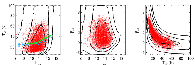
The results of our variable-$T$ and $\beta$ fitting are shown in figure 1, with stacked 1D PDFs for $L_{\mathrm{dust}}$, $T_{\mathrm{eff}}$ and $\beta_{\mathrm{eff}}$ in figure 1 (a), and contour plots of the stacked two-dimensional PDFs for the three different combinations of parameters shown in figure 1 (b), in which median-likelihood values for each galaxy are overlaid in red. We also overlay the dust luminosity-temperature relations from Chapman et al. (2003) and Hwang et al. (2010) in light blue and green, respectively.

Allowing both isothermal temperature and emissivity index to vary in our fitting on a galaxy-by-galaxy basis gives several interesting results. As figure 1 (a) shows, the range of values for $L_{\mathrm{dust}}$ appears quite reasonable, even when marginalising over such a large range of temperatures and emissivities, while the range of derived temperatures and emissivity indices is considerably larger than can be found in the literature (despite the fact that we do not explore the impact of alternative greybody SED parametrisations on our results, and use the standard form given in equation 1 throughout). Though literature values for emissivity indices typically vary between at most $1.0<\beta<2.5$, we find that the range of values supported by the H-ATLAS data using this method is extremely broad, though this (in contrast to the sensible range of values for $L_{\mathrm{dust}}$, consistent with that observed in H-ATLAS using full multiwavelength SED-fitting by e.g. Smith et al., 2012) is hardly surprising given that the majority of sources in our sample are only well-detected (i.e. $\geq 5\sigma$) in the 250 $\mu$m band 1. Interestingly, we also derive a strong anti-correlation between $T_{\mathrm{eff}}$ and $\beta_{\mathrm{eff}}$ using this method, in apparent agreement with the results of (e.g. Chapman et al., 2003; Désert et al., 2008; Anderson et al., 2010; Veneziani et al., 2010; Planck Collaboration et al., 2011).

(a) Stacked marginalised one-dimensional PDFs for $L_{\mathrm{dust}}$, $T_{\mathrm{eff}}$, and emissivity index, $\beta$.

(b) Two-dimensional stacked PDFs for the various combinations of $L_{\mathrm{dust}}$, $T_{\mathrm{eff}}$ and $\beta$.

Figure 1: The (top) one- and (bottom) two-dimensional stacked PDFs for the galaxies in our sample which are well-described by the simple greybody model (i.e. those with reduced $\chi^{2}<2.0$). In the bottom panel, the median-likelihood esimates for each source are overlaid as the red points, while the “L-T” relations from Chapman et al. (2003) and Hwang et al. (2010) are shown as the light-blue and green lines, respectively.

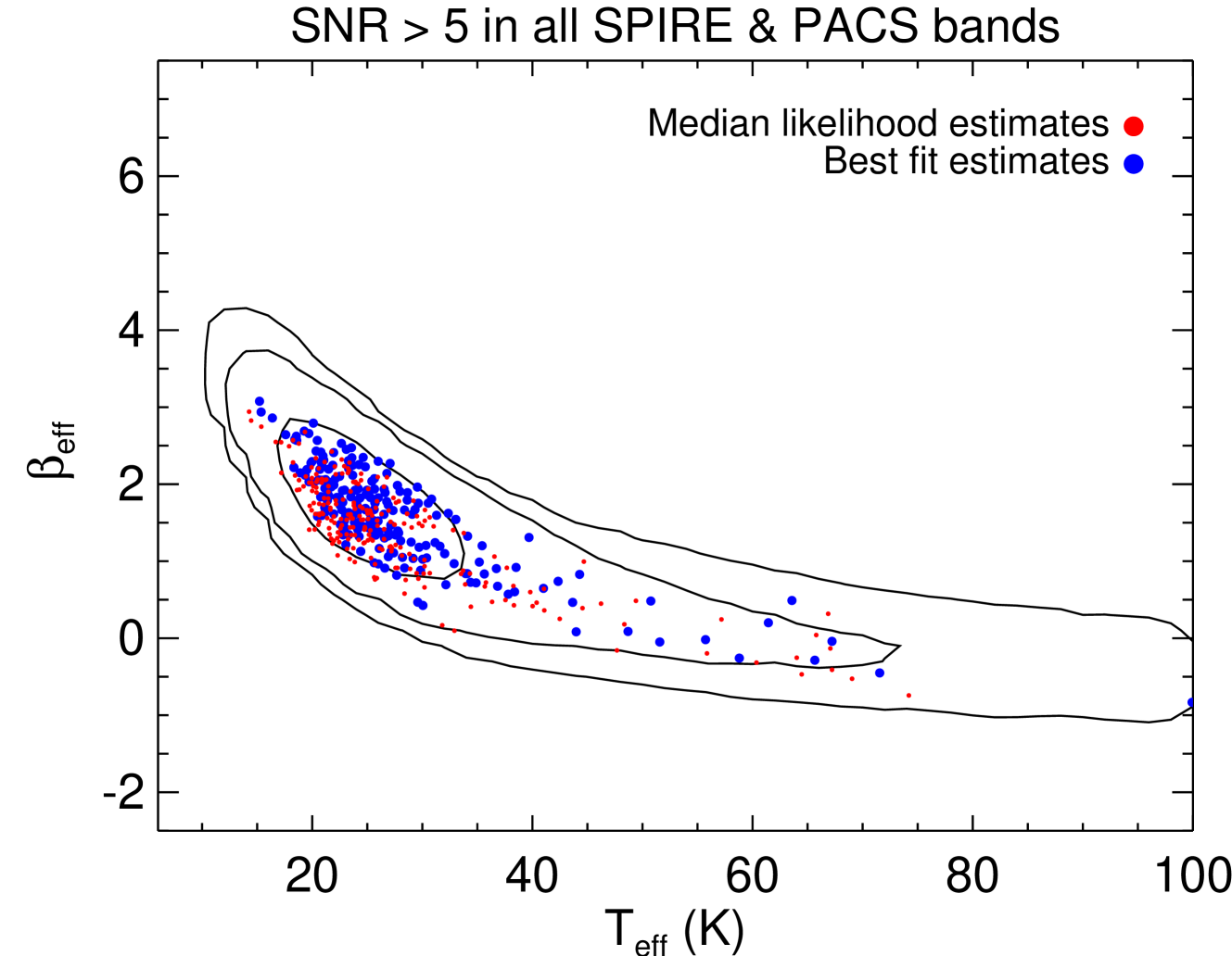
It is common practice to limit a sample to only include those sources detected at the highest signal-to-noise ratio, in order to derive the best constraints on parameters of interest. In H-ATLAS we have 238 galaxies which have photometry with signal to noise ratios $\geq 5.0$ in the “BEST” catalogue photometry in each of the PACS and SPIRE bands. We show the results of applying our fitting technique to these galaxies in figure 2, and once more recover an apparently convincing anti-correlation between these two parameters.

Figure 2: The relationship between $T_{\mathrm{eff}}$ and $\beta_{\mathrm{eff}}$ for only those 238 sources with the best photometry in H-ATLAS, with the best-fit (blue) and medium-likelihood (red) values overlaid on the 68.3, 95.5, and 99.7 per cent confidence contours (i.e. equivalent to the 1, 2, and $3\sigma$ levels assuming Gaussian statistics, in black).

3.2 Validation; simulations

Shetty et al. (2009a) suggested that an anti-correlation between isothermal temperature and $\beta$ arises inevitably through the influence of instrumental noise on simple $\chi^{2}$ fitting, and in a partner publication (Shetty et al., 2009b) through the presence of multiple dust temperatures superposed along the line of sight (see also Veneziani et al., 2013). To test whether the former result affects H-ATLAS, we conducted a set of simple simulations designed to inform our studies of $L_{\mathrm{dust}}$, $T_{\mathrm{eff}}$ and $\beta_{\mathrm{eff}}$ based on the H-ATLAS data set.

To populate our simulation, we first chose 200,000 temperatures, randomly distributed between $11<T_{\mathrm{eff}}\ <56$ K, and assigned each temperature an emissivity index drawn at random from a Gaussian distribution with median $\beta=1.98$ and $\sigma(\beta)=0.25$, allowing us to generate a model intrinsic spectrum for each source. We then computed the transmission of each model spectrum through the PACS and SPIRE response functions to generate model noiseless photometry in each of our photometric bands. Every model source in our simulation now has an assigned temperature and emissivity index, leaving only the normalisation of the model remaining to be determined.

To avoid making any assumptions about the source number counts in H-ATLAS, we assume that the observed fluxes of the model sources in our catalogue (which in reality are a sum of the true flux from that source, with additive noise based on the properties of the observations in each band) are drawn from among the sources in the H-ATLAS catalogue. We simulate the noise contribution to the measured flux in each band differently for the PACS and SPIRE observations; for PACS we generate a Gaussian distribution of noise values with standard deviation equal to the 1$\sigma$ noise in the catalogues. In the SPIRE bands, however, there is an additional contribution to the noise component of the measured flux from source confusion (which increases with wavelength; Nguyen et al., 2010; Rigby et al., 2011), making the true noise distributions asymmetric. To model the SPIRE noise properties, we read off values at random positions from the PSF-smoothed maps at 250, 350, and 500 $\mu$m, automatically including the instrumental and confusion noise components.

Using these model noise realisations, we determine the “true” 250 $\mu$m flux for each model source (i.e. the flux we would measure in the absence of noise) and calculate the normalisation for each model dust SED to the true 250 $\mu$m flux density using equation 2:

$$\hat{S}_{250}^{\mathrm{model}}=\hat{S}_{250}^{\mathrm{obs}}-\hat{E}_{250}^{\mathrm{model}}.$$ (2)

Where $\hat{E}_{250}^{\mathrm{model}}$ is the array of model noise values measured from the 250 $\mu$m maps, $\hat{S}_{250}^{\mathrm{obs}}$ is the array of observed 250 $\mu$m fluxes drawn from H-ATLAS and $\hat{S}_{250}^{\mathrm{model}}$ is the precise intrinsic flux of each model source. Calculating this “noiseless” 250 $\mu$m flux density for each source allows us to normalise each model dust SED according to the noiseless value, and then by inverting equation 2, “add back on” the noise model for each of the normalised PACS and SPIRE bands. In this way, we recover the observed H-ATLAS 250 $\mu$m flux density distribution exactly, and generate model photometry in the other four PACS and SPIRE bands with realistic noise characteristics. To ensure that our error estimates are consistent with those in H-ATLAS, we assign an error on each noisy model photometric data point by adopting the quoted error on the most closely corresponding source in terms of flux density in the real H-ATLAS catalogue on a band-by-band basis.

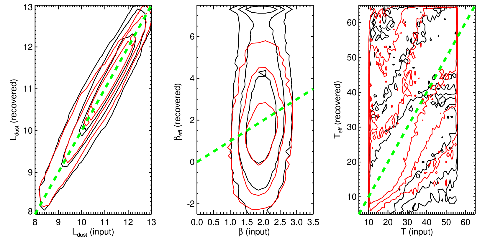
In figure 3 we show the variation between the known input values in our simulation and the results of our attempts to recover them. The red contours in figure 3 show the variation of the median-likelihood estimates of $L_{\mathrm{dust}}$, $\beta_{\mathrm{eff}}$ and $T_{\mathrm{eff}}$, whilst the black contours show the best-fit values (the contour levels represent 1, 2 & 3$\sigma$ confidence levels in both cases). Though both methods produce reasonable estimates of total dust luminosity, the same can not be said of our attempts to recover either $\beta_{\mathrm{eff}}$ or $T_{\mathrm{eff}}$, which display large discrepancies from their known input values, though the best-fit values show greater bias with larger uncertainties than the median-likelihood values. This discrepancy from the input values is in stark contrast to the results of section 5, in which we will derive temperatures and luminosities at fixed emissivity index; clearly allowing $\beta$ to vary has important implications for our results.

Figure 3: Comparisons between the input values for $L_{\mathrm{dust}}$, $\beta$ and $T_{\mathrm{eff}}$ (left, centre and right-hand panels, respectively) and their median-likelihood (red) or best-fit (black) esimates in our H-ATLAS-like simulation. The contour levels correspond to the regions enclosing 68.3, 95.5 and 99.7 per cent of the recovered values. The green dashed lines indicate the ideal relation between input and recovered values, and the excess of best-fit sources around $\beta_{\mathrm{eff}}$ (recovered) $\approx 7.5$ in the centre panel results from the tendency of best-fit values to accumulate where the posterior probability distribution is truncated by the bounds of the prior.

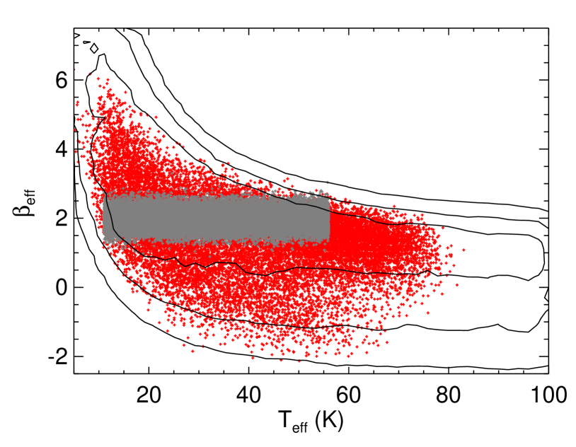
To investigate the large discrepancies between the input and output temperatures and emissivity indices, in figure 4 we show the relationship between $T_{\mathrm{eff}}$ and $\beta_{\mathrm{eff}}$ for the sources in our simulation, with the input values in grey, the derived median-likelihood values in red, and the contours representing the stacked 2D PDF in black. Though the intrinsic relationship between temperature and emissivity index in our simulation is flat, the noise on our simulated photometry causes an artificial temperature–emissivity index anti-correlation to be recovered. This is in agreement with the results of Shetty et al. (2009a) and more recently Galametz et al. (2012), and explains the contrast between the input and derived parameters in figure 3.

Figure 4: Two dimensional stacked probability density function for $T_{\mathrm{eff}}$ and $\beta$ shown by the solid black contours indicating the regions enclosing 68.3, 95.5 and 99.7 percent of the PDF. The median-likelihood estimates for each simulated galaxy well-described by our model are shown as the red points with the overlaid grey points indicating the input values, revealing the extent of the artificial anti-correlation.

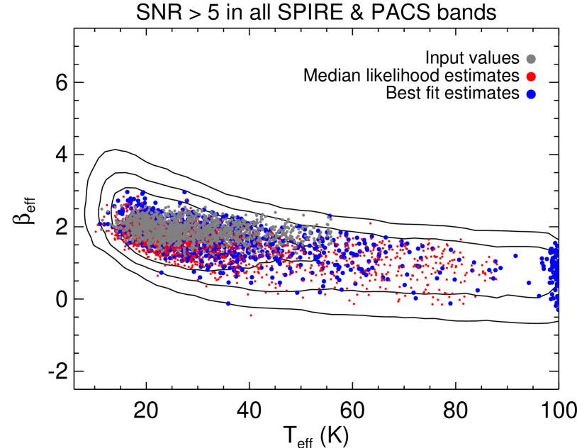
As mentioned in section 3.1, it is common practice to limit a sample to include only those sources with the highest signal-to-noise ratios in their photometry. We now use our simulation to test whether this approach can mitigate the influence of the anti-correlation. Figure 5 shows the relationship between the derived temperature and emissivity index including only those simulated sources with $\geq 5\sigma$ detections in each of the PACS and SPIRE bands. Once more the input values are shown in grey, while the best fit values are shown in blue, with the median-likelihood estimates in red. Though the range of recovered $\beta_{\mathrm{eff}}$ is unsurprisingly smaller than for the full sample, the artificial anticorrelation still persists, though the range of temperatures input to the simulation is broader than is observed in H-ATLAS (our input distribution of model temperatures is flat between $11\leq T_{\mathrm{eff}}\leq 56$ K).

Figure 5: Comparison between the values of temperature and emissivity index input to our simulation (grey points) and derived using best-fit (blue) and medium-likelihood (red) estimators. The clump of blue points reflects the tendency for best-fit values to be returned on the bounds of the temperature prior when the prior truncates the PDF. In contrast to figure 4, this plot shows only sources with $\geq 5\sigma$ detections in each PACS/SPIRE band.

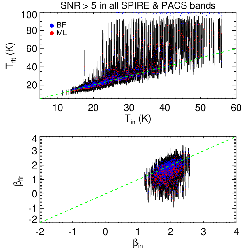
To highlight the bias, in figure 6 we show the relationship between the individual recovered $T_{\mathrm{eff}}$ and $\beta_{\mathrm{eff}}$ and their corresponding input values. The median likelihood values are shown as the red circles with the black error bars corresponding to the 16th and 84th percentiles of the individual PDFs, while the best-fit values are shown as the blue circles. The recovered temperatures show considerable bias above their input values (represented by the dashed green line) and the emissivity indices are biased low even when considering only the galaxies with the highest SNR in our simulated PACS/SPIRE photometry.

Figure 6: A comparison between the input and derived temperatures (top) and emissivity indices (bottom), for simulated sources with $\geq 5\sigma$ detections in each of the PACS/SPIRE bands, with unity highlighted using the dashed green line. The red circles with errors represent the median-likelihood estimates, while the blue points represent the best-fit values. It is clear that when both $T_{\mathrm{eff}}$ and $\beta_{\mathrm{eff}}$ are allowed to vary, temperatures are inevitably biased high, and emissivity indices show considerable negative bias.

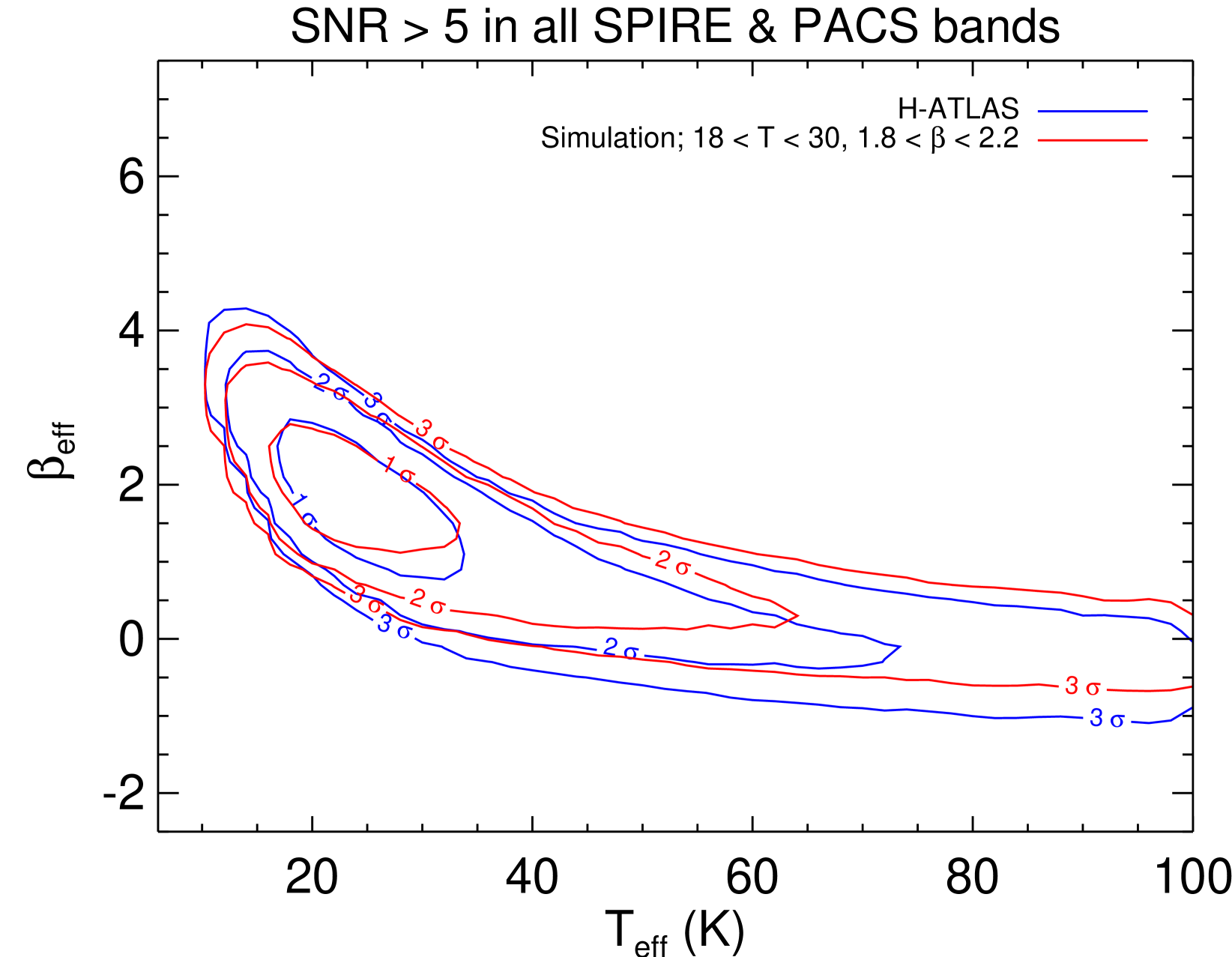
Finally, if we reduce the range of the input values for temperature and emissivity index that have gone in to our model sample, such that $18.0\leq T\leq 30.0$ and the Gaussian distribution of emissivity indices is truncated at $1.8\leq\beta\leq 2.2$, and again select only those sources with $\geq 5\sigma$ detections in each Herschel band, we recover results very similar to those recovered using the corresponding subsample (in SNR) of the real H-ATLAS data set, despite there being no intrinsic correlation between $\beta$ and $T$. Figure 7 shows the 1, 2, and $3\sigma$ confidence intervals of the 2D PDF for the highest-SNR subset of H-ATLAS (in blue) and of our simulation (in red).

Since we have shown that we recover an apparent anti-correlation between temperature and emissivity index, even though the two are independent in the simulated data and despite having included only those sources with the best-constrained SEDs, it is clear that any evidence for correlation between $T_{\mathrm{eff}}$ and $\beta_{\mathrm{eff}}$ derived using this method is weak.

Figure 7: Comparison between the 2D confidence intervals for $T_{\mathrm{eff}}$ and $\beta_{\mathrm{eff}}$ shown for the subset of the H-ATLAS catalogue detected at $\geq 5\sigma$ in all PACS/SPIRE bands (in blue) and for a similar subset of our simulation (in red), with the input values of temperature and emissivity truncated relative to the full simulation, as discussed in the text. The values input to our simulation for $T_{\mathrm{eff}}$ and $\beta_{\mathrm{eff}}$ have no intrinsic correlation.

4 What are the parameters of the average isothermal H-ATLAS galaxy SED?

4.1 Method

As we mentioned in the introduction, use of standard values for emissivity index and temperature of model far-infrared isothermal SEDs is common at all redshifts; with this in mind, it is desirable to determine our best global estimates of the temperature and emissivity index for galaxies in H-ATLAS assuming this model.

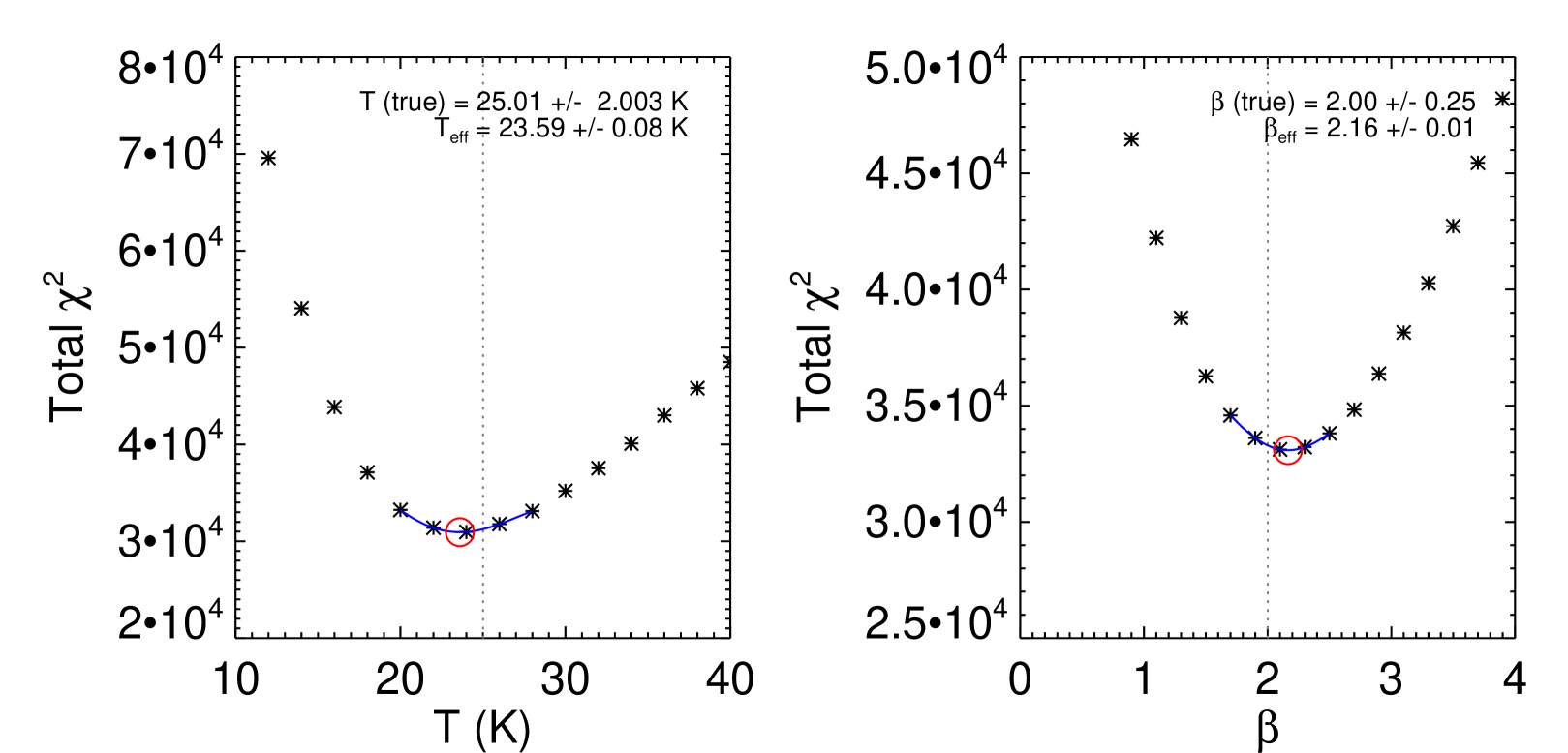
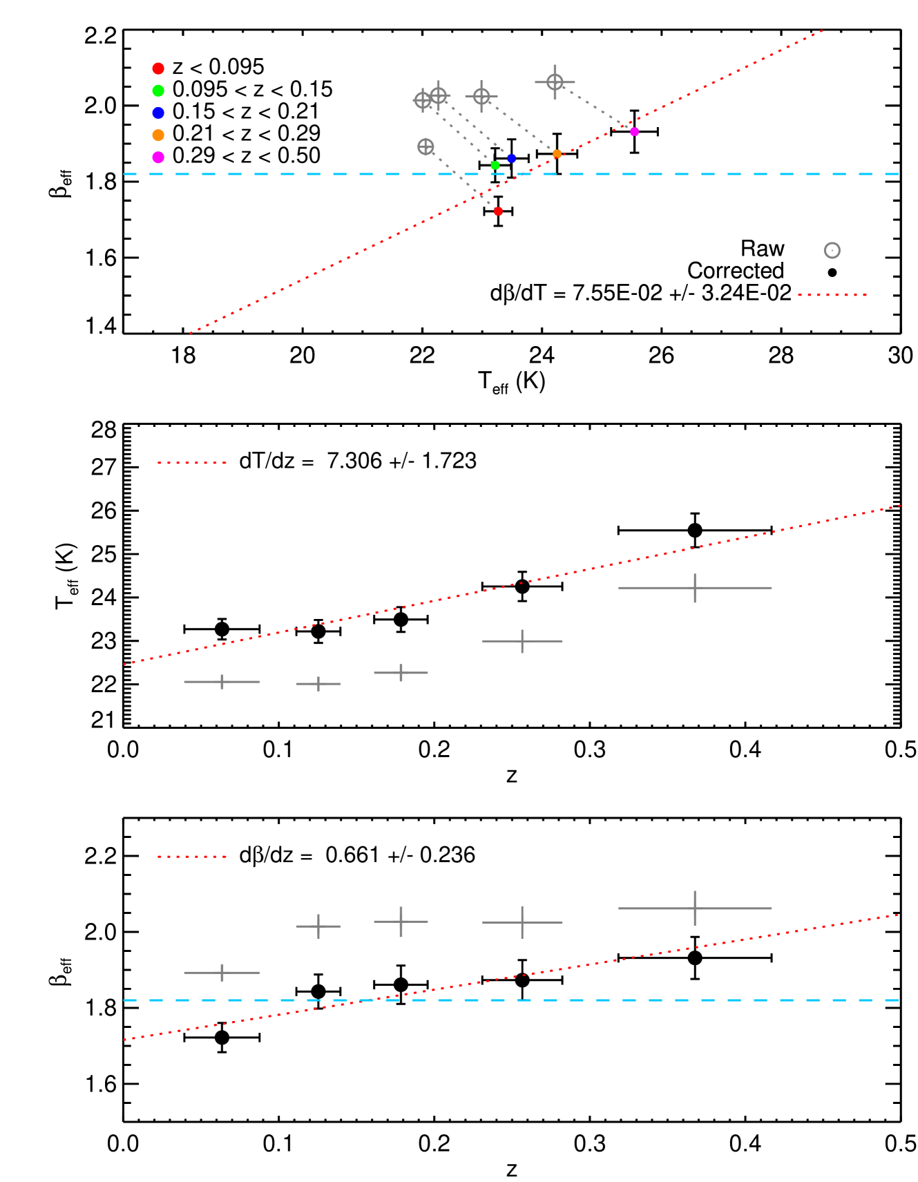
Clearly, the artificial anti-correlation produced by the $\chi^{2}$ fitting precludes producing useful results on a galaxy-by-galaxy basis using this technique. We use a simple method, similar to that used by Hardcastle et al. (2013), to determine the best-fit global $T_{\mathrm{eff}}$ and $\beta_{\mathrm{eff}}$. To do this, we treat the galaxies in H-ATLAS as a homogeneous sample, and record the best-fit $\chi^{2}$ value in bins of $\beta_{\mathrm{eff}}$ allowing $T_{\mathrm{eff}}$ and $L_{\mathrm{dust}}$ to vary (and similarly in bins of $T_{\mathrm{eff}}$ allowing $\beta_{\mathrm{eff}}$ and $L_{\mathrm{dust}}$ to vary). We may then calculate the sum of the $\chi^{2}$ values in each bin across the good fits in our sample (i.e. those galaxies with $\chi^{2}_{\mathrm{best}}<2.0$). This technique has the advantage that by summing in $\chi^{2}$, those galaxies with only weak constraints from the photometry have approximately flat distributions of $\chi^{2}(T_{\mathrm{eff}})$ and $\chi^{2}(\beta_{\mathrm{eff}})$, while those galaxies with the best constraints exhibit clear minima in these distributions, which when combined over the whole sample produce strongly preferred values of $T_{\mathrm{eff}}$ and $\beta_{\mathrm{eff}}$. Furthermore, this approach not only increases the signal-to-noise ratio by combining together the photometry for all of the sources in a sensible way, but also naturally accounts for the asymmetric error distributions for each individual source, which preclude using a traditional weighted mean approach. Stacking the values of $\sum\limits_{i}\chi_{i}^{2}(T_{\mathrm{eff}})$ and $\sum\limits_{i}\chi_{i}^{2}(\beta_{\mathrm{eff}})$ results in a naturally weighted distribution allowing us to derive our best estimates of the two parameters.

Our model library contains 50,000 stochastic samplings of $\beta_{\mathrm{eff}}$ and $T_{\mathrm{eff}}$ in each redshift bin (recall that our library samples redshift at $\Delta z=0.01$ for $0.00<z<0.50$); in order that our histograms of $\chi^{2}(T_{\mathrm{eff}})$ and $\chi^{2}(\beta_{\mathrm{eff}})$ are smoothly-varying, we use a resolution of $\Delta T_{\mathrm{eff}}=2.0$ K, and $\Delta\beta_{\mathrm{eff}}=0.2$. Since the sampling in temperature and emissivity index in our histograms is relatively coarse, we assume that the underlying distributions of $\chi^{2}$ are also smoothly varying, and locate the minimum of each distribution by interpolating the five data points about the minimum using a fourth order polynomial. We may then use the polynomial fit to the total $\chi^{2}$ distribution to generate PDFs for $\beta_{\mathrm{eff}}$ and $T_{\mathrm{eff}}$ in our sample by assuming the same relationship between probability and $\chi^{2}$ as before. We derive uncertainties using the 16th and 84th percentiles of the resulting PDF. Due to the large number of sources in the sample, and the large values of $\chi^{2}$ in each bin, the derived errors are smaller than the histogram bins, reflecting the need to interpolate between them. Finally, in contrast to the results for individual galaxies, the maximum- and median-likelihood values that we derive using this method are very similar since the PDFs obtained from the polynomial fits to the histograms of $\sum\limits_{i}\chi^{2}_{i}$ are very well constrained.

In figure 8 we show examples of the results of using this method to determine our best estimates of the population mean $T_{\mathrm{eff}}$ and $\beta_{\mathrm{eff}}$, to compare the results with the known input values from a similar simulation to the one discussed in section 3.2. However, since we are now interested in the global properties of galaxies in H-ATLAS rather than determining the bias in our fitting techniques, we assume input values to our simulation which are Gaussian-distributed about $\beta=2.00\pm 0.25$ and $T_{\mathrm{eff}}=25.0\pm 2.0$, uncorrelated with $\beta$. The left-hand panel of figure 8 shows typical results derived using $\sim$14,000 model galaxies described using the isothermal model. Though using this technique limits the influence of the aforementioned artificial anti-correlation introduced through line-of-sight effects and noisy photometry, the derived values for $\beta$ (left panel) still show residual systematic bias towards higher values, while $T_{\mathrm{eff}}$ (right) still shows slight bias towards colder temperatures than the inputs.

Figure 8: Plots illustrating the method for recovering known values of $T_{\mathrm{eff}}$ and $\beta$ using our technique. We sample $\beta$ (left) and temperature (right) and calculate the total $\chi^{2}$ over the whole sample in each bin. We model the $\chi^{2}$ distribution about the bin with the lowest value, using a fourth order polynomial (in blue), and find the minimum value by interpolating along this polynomial and assuming that the distribution of values in $\chi^{2}$ space is smooth. The determined minimum is shown by the red circles in each plot, with the true values for this particular library ($\beta=2.00\pm 0.25$ and $T_{\mathrm{eff}}=25.0\pm 2.0$) indicated by the vertical dashed grey lines.

To illustrate this method, and better quantify the bias, we show the results of recovering the known input values on 100 Monte-Carlo realisations of a grid of Gaussian distributed temperatures about 15, 20 and 25 (all $\pm\ 2$ K), and uncorrelated $\beta=1.5$, 2.0 and 2.5 (all $\pm 0.25$) in figure 9. We also include another input sample arbitrarily centred on $T_{\mathrm{eff}}=23.2\pm 5.0$ K and $\beta_{\mathrm{eff}}=1.88\pm 0.50$ to show that the results are reasonable for broad as well as narrow distributions of $T_{\mathrm{eff}}$ and $\beta_{\mathrm{eff}}$. The results of recovering $T_{\mathrm{eff}}$ are shown in the left panels, while the results for $\beta_{\mathrm{eff}}$ are shown on the right. The values of $T_{\mathrm{eff}}$ recovered by our fitting of this simulation ($T_{\mathrm{fit}}$) are consistently biased lower than the input values ($T_{\mathrm{in}}$), with the best fit linear relationship (thick grey line) biased below the ideal relationship (dashed grey).

The best-fit linear relationship between input and recovered temperatures (the solid line in figure 9), under the assumptions that $T_{\mathrm{eff}}$ and $\beta_{\mathrm{eff}}$ are independent, and Gaussian distributed about some mean value, is given by equation 3:

$$T_{\mathrm{fit}}=(0.949\pm 0.001)T_{\mathrm{input}}+(0.023\pm 0.039).$$ (3)

This relationship does not show any strong dependence on the value of $\beta$ in the simulation, reflected by the coloured points and error bars in the left-hand panels in figure 9 which are all consistent with equation 3 (the thick grey line).

Figure 9: Recovering temperatures (left) and $\beta$ values (right) using our technique applied to 100 realisations of ten combinations of temperature and emissivity index. The input values are spaced on a grid of $T_{\mathrm{eff}}$ and $\beta$, with $T_{\mathrm{eff}}$ = 15, 20 and 25 K and $\beta=1.5$, 2.0 and 2.5 as shown by the coloured points (see legend), and each simulation assumes that temperature and emissivity index are independent and Gaussian distributed; the derived errors in the recovered values are smaller than the plotting symbols. We also include a broader distribution of input temperatures and emissivities centred about $T_{\mathrm{eff}}=23.18\pm 6.1$ and $\beta=1.88\pm 0.5$ to demonstrate the validity of our approach for both narrow and wide input distributions. The dashed grey line shows the ideal relation (i.e. perfect recovery of each parameter) in both the left and the right panels. The thick grey line in the left panel shows the best fit linear relationship between the input and output temperatures as detailed in equation 3. The dashed coloured lines in the right-hand plot (for the recovery of $\beta$) show the best-fit linear relationship between the input and derived values in bins of input temperature. We correct for this offset as a function of temperature using equation 4, as described in the text.

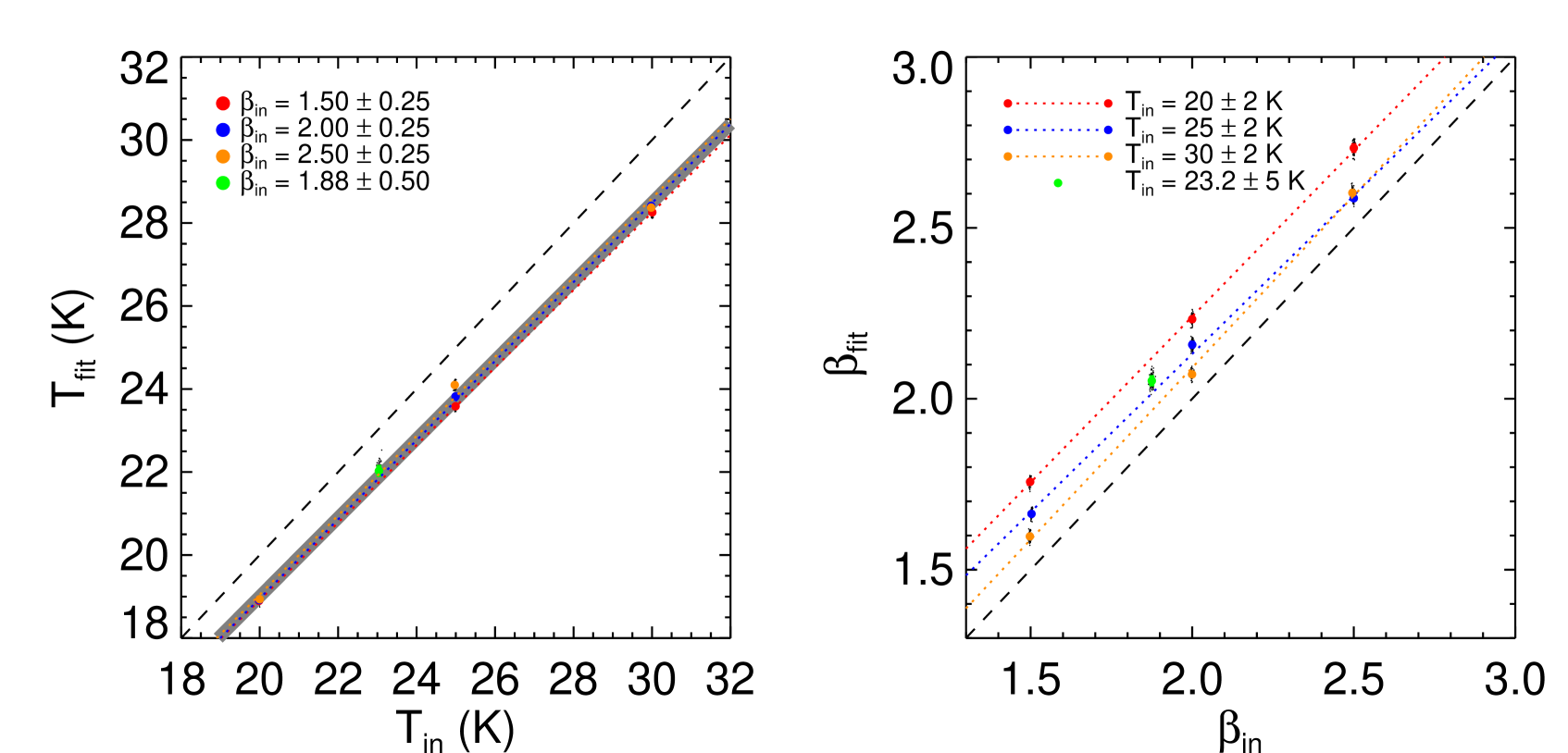
Our results for recovering $\beta$ are more complicated, with the bias to higher emissivity indices being more pronounced for the colder sources on the model grid, and the corresponding offsets between the coloured dotted lines (the best-fit linear relationships for each input temperature bin). We show the temperature dependence of the $\beta$-bias in figure 10, with each point representing one of 100 Monte-Carlo realisations sampling 14,000 model galaxies. We show the bias as a function of input temperature in black, and as a function of the recovered temperatures, after correcting for the fitting offset using equation 3, overlaid in green. To quantify the bias in $\beta$ as a function of $T_{\mathrm{eff}}$, we derive a 2nd-order polynomial fit between the corrected temperatures and $(\beta_{\mathrm{fit}}-\beta_{\mathrm{input}})$, with the values for each parameter shown in the upper right-hand corner of figure 10. The best fit 2nd-order polynomial is given by equation 4:

$$\begin{split}\beta_{\mathrm{fit}}-\beta_{\mathrm{input}}=\ &(1.28\pm 0.28)\times 10^{-3}\ T_{\mathrm{cor}}^{2}\\ &-(7.93\pm 1.38)\times 10^{-2}\ T_{\mathrm{cor}}\\ &+(1.32\pm 0.17).\end{split}$$ (4)

As a crude test of whether combining the galaxies in this way limits the impact of anti-correlation on our results as compared with a more traditional fitting approach, we compare the degree of anti-correlation recovered by the two methods.

Figure 10 reveals a change of $\Delta\beta\approx 0.15$ between $T=20--30$ K ($\Delta\beta/\Delta T\approx 0.015$), whilst the traditional $\chi^{2}$ fitting (figure 4) suggests a change of $\Delta\beta\approx 1$ over a similar range of temperature ($\Delta\beta/\Delta T\approx 0.1$). These values suggest a factor of $>6$ times improvement in terms of the influence of the anti-correlation (though at the expense of estimates of $T_{\mathrm{eff}}$ and $\beta_{\mathrm{eff}}$ for the individual sources). This is perhaps even more notable given that we do not account for confusion noise in our SED fitting.

Figure 10: The difference between the values for $\beta$ inserted in to and recovered from one hundred realisations of our simulations, as a function of the recovered “corrected” temperature (in green) and the true (i.e. input) temperature (in black). The best 2nd order polynomial fit to $\beta_{in}-\beta_{fit}$ as a function of corrected recovered temperature is overlaid as the dotted grey line, with the fit parameters detailed in the legend, and in equation 4.

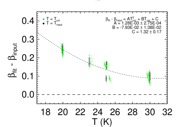
We assume uncertainties on the corrected temperatures and emissivity indices equal to the standard deviation of the corrected values (derived using equations 3 & 4) about their medians, added in quadrature to the mean of the 16th and 84th percentiles of the derived PDFs.

It is tempting to use these offsets based on our simulations to crudely attempt to correct for the bias in the derived values of $T_{\mathrm{eff}}$, however, these offsets are only really valid for the particular case in which $\beta_{\mathrm{eff}}$ is independent of $T_{\mathrm{eff}}$; to test the strength of this assumption, we generated additional suites of simulations in which $T_{\mathrm{eff}}$ and $\beta_{\mathrm{eff}}$ have plausible intrinsic correlation or anti-correlation. When we attempt to recover the input values using our method on the correlated simulations, the offsets we recover are $\Delta T_{\mathrm{eff}}=T_{\mathrm{recovered}}-T_{\mathrm{true}}=-1.51\pm 0.11$ K and $-0.71\pm 0.13$ for the anti-correlated and correlated simulations, respectively, as compared with $\Delta T_{\mathrm{eff}}=-1.14$ assuming equation 3, suggesting that our temperature corrections are reasonable to within $\sim 0.4$ K. For $\Delta\beta_{\mathrm{eff}}$ (defined in the analogous manner), the values we recover are $0.00\pm 0.02$ and $0.16\pm 0.02$, as compared with $\Delta\beta_{\mathrm{eff}}=0.18$ estimated using equation 4.

Since we have shown that previous studies inevitably produced artificially anti-correlated values of $T_{\mathrm{eff}}$ and $\beta_{\mathrm{eff}}$ using this technique, and the best estimate of the variation between $T_{\mathrm{eff}}$ and $\beta_{\mathrm{eff}}$ not subject to this limitation finds only weak positive correlation between the two (Kelly et al., 2012, albeit over a very small temperature range, and with a large range of $\beta$ at any given temperature; see the right-hand panel of their figure 6), we proceed under the assumption that the two are effectively un-correlated in H-ATLAS, though in what follows we quote both the raw and the crudely “corrected” values.

4.2 Global dust properties in H-ATLAS

We applied our method to the stacked $\chi^{2}$ distributions of the 12,814 out of 13,826 galaxies with best-fit reduced $\chi^{2}<2.0$. The results are shown in figure 11; the median likelihood values for 250 $\mu$m-selected galaxies are $T_{\mathrm{eff}}=22.3\pm 0.1$ K and $\beta_{\mathrm{eff}}=1.98\pm 0.02$. If we use equations 3 & 4 to correct these values in the same way as before (again highlighting that these corrections assume independent $T_{\mathrm{eff}}$ and $\beta_{\mathrm{eff}}$, and that the true values are normally distributed) we derive our best estimates for galaxies in H-ATLAS of $T_{\mathrm{eff}}^{\mathrm{corr}}=23.5\pm 0.1$ K and $\beta_{\mathrm{eff}}^{\mathrm{corr}}=1.82\pm 0.02$. Our estimate of $\beta$ compares well with the results of Planck Collaboration et al. (2011), who suggest a distribution centred about $\beta=1.78$ (albeit with “significant T-$\beta$ anti-correlation”). It is also consistent with the ranges of values suggested by Chapin et al. (2009); Paradis et al. (2010); Bracco et al. (2011); Liang et al. (2012); Galametz et al. (2012); Magnelli et al. (2012) and Roseboom et al. (2013) for a wide range of sources, including galactic star forming regions, galactic cirrus, resolved nearby galaxies and high redshift sub-millimetre galaxies; that the values for $\beta$ are consistent over such a wide variety of scales is remarkable.

Figure 11: SED fitting results for emissivity index $\beta$ and $T_{\mathrm{eff}}$ in H-ATLAS, showing the distributions of $\sum\chi^{2}(\beta)$ and $\sum\chi^{2}(T)$. The data are shown as black asterisks, while the best-fit fourth-order polynomial is shown as the blue line, with the location of the minimum (i.e. the best-fit) shown by the red circle, with the uncorrected values for each minimum quoted in the legend. The similarity of these values to those derived for our simulation in figure 8 indicate the fidelity of our simulation to H-ATLAS.

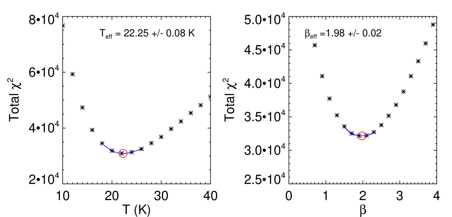
In figure 12 we show the results of applying our fitting method once more, this time in bins of redshift, to test for the possibility of variation in emissivity index or $T_{\mathrm{eff}}$. A suite of simulations, similar to those discussed in section 3.2 only with bins containing 2,600 objects, were found to have $T_{\mathrm{eff}}$ and $\beta_{\mathrm{eff}}$ offset from their input values in a manner consistent with equations 3 and 4 derived using 14,000 objects per bin (albeit with larger uncertainties). We use the same corrections for these values, and update the uncertainties accordingly.

The bounds of the redshift bins, as well as the gradient of the best-fit linear fit to each combination of parameters (in orange) are detailed in the panel legends. In the top panel, we show that there is only weak evidence for variation in $\beta_{\mathrm{eff}}$ as a function of $T_{\mathrm{eff}}$ and of redshift (or dust luminosity; the median dust luminosity in each redshift bin is given in the caption to figure 12), with the gradient of the linear best fit relationship distinct from zero only at the $\sim 2.3\,\sigma$ level. This large uncertainty reflects the possibility that the relationship may be largely driven by a single outlying bin (perhaps either the highest or lowest redshift bin); it is quite possible that the highest redshift bin is biased towards higher temperatures due to the higher average dust luminosity of the sources in this bin (i.e. Malmquist bias) combined with the aforementioned “L-T” relation. In the middle plot we show the redshift variation of $T_{\mathrm{eff}}$, showing a weak trend as expected from the “$L-T$” relations suggested in previous works and overlaid in figure 1; the gradient is significant at the 4.2 $\sigma$ level. The median dust luminosity in each redshift bin also increases with redshift, as expected. In the bottom panel, we compare the derived emissivity indices with the best-fit value across the whole sample (dashed light-blue line), again showing only weak evidence for any variation (the gradient of the best-fit line, shown in dotted orange, is formally only significant at the 2.8 $\sigma$ level).

Though we have attempted to correct for residual bias in our results using equations 3 and 4, these corrections are invalid if the two are related (a hypothesis for which there is only weak statistical evidence at the time of writing, though our simulations in section 4 suggest that the additional uncertainty added to the corrections in this case is only $\sim 0.4$ K or a change in emissivity of around 0.18). We leave further investigation of any putative intrinsic relation between $T_{\mathrm{eff}}$ and $\beta_{\mathrm{eff}}$ for a future investigation.

Figure 12: Top: Comparison between the values derived using our method for $T_{\mathrm{eff}}$ and $\beta$ in bins of redshift, such that there are approximately equal numbers of galaxies in each bin. Middle: Variation between the recovered $T_{\mathrm{eff}}$ as a function of redshift, showing a $>4\sigma$ positive correlation. Bottom: recovered $\beta$ as a function of redshift, showing only weak evidence for redshift dependance of emissivity index in H-ATLAS. The median $\log_{10}\left(L_{\mathrm{dust}}/L_{\odot}\right)$ for each redshift bin is 10.01, 10.42, 10.67, 10.97 and 11.31, from the lowest to the highest redshift bin, respectively.

5 Recovering temperature and luminosity at fixed emissivity index using H-ATLAS

Using isothermal models to describe the far-IR properties of H-ATLAS sources holds the distinct advantage of enabling us to compare dust temperatures with pre-Herschel studies. As we explained in the previous sections, it is common for emissivity index to be held fixed, since effective temperatures can be useful even with a small number of data points available to constrain the far-infrared SED. In what follows, we assume a fixed emissivity index, $\beta=1.82$ corresponding to our best estimate of the global mean in H-ATLAS, after correcting for bias as discussed in the previous section. We will discuss the implications of the choice of $\beta$ in section 6.

We perform $\chi^{2}$ minimisation comparing each galaxy in our sample to a library of model photometry, based on dust SEDs derived using equation 1, evaluated on a grid of temperatures between $5.0<T_{\mathrm{eff}}\ <65$ K at 0.2 K resolution. Once more, we account for the transmission of each dust spectrum through the PACS and SPIRE response functions, and build $T_{\mathrm{eff}}$ and $L_{\mathrm{dust}}$ PDFs for each galaxy in the same manner as before. We calculate best-fit values, and use the PDFs to determine median-likelihood estimates of $T_{\mathrm{eff}}$ and $L_{\mathrm{dust}}$ as well as uncertainties, in the same manner as before.

To test the ability of our fitting to recover $T_{\mathrm{eff}}$ and $L_{\mathrm{dust}}$ of galaxies in H-ATLAS, we also built a fixed $\beta=1.82$ version of the H-ATLAS-like simulation mentioned above, and generated three additional closely-related simulations:

• We re-ran the simulation neglecting the SPIRE confusion noise from the modelling, instead using a symmetric Gaussian model noise distribution rather than the asymmetric combination of instrumental and confusion noise that blights the real data. The standard deviation of the symmetric model noise distribution is defined to be equal to the sum in quadrature of the instrumental and confusion noise distributions in the real H-ATLAS data set (i.e. the values quoted in section 2).

• We repeated simulating the model photometry, this time assuming that the PACS data have the same sensitivity as the SPIRE 250 $\mu$m data, to compare our results with those available using the greater sensitivity available using other, smaller area Herschel surveys, in particular the combination of the PACS Evolutionary Probe (PEP; Lutz et al., 2011) and the Herschel Multi-tiered Extragalactic Survey ($Her$MES; Oliver et al., 2012). We note that the only difference between this simulation and the “H-ATLAS-like” simulation (previous item in this list) is the sensitivity of the PACS data, not the observed source counts.

• Finally, we generated a simulation neglecting the PACS data, to test our ability to recover temperatures using the SPIRE photometry alone.

The results of fitting to these different simulated datasets are discussed in the following subsections. The flat input distribution of temperatures in our simulation enables us to test the ability of our fixed $\beta$ $\chi^{2}$ fitting to recover galaxies across a large range of temperature and dust luminosity. It is not intended to be consistent with the H-ATLAS selection function, merely to enable us to study the biases inherent in using different data sets to study these parameters.

5.1 Recovering known temperature and luminosity

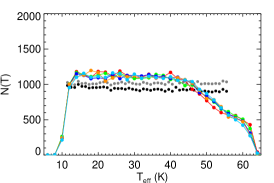
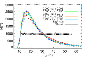
For each set of simulations, we wanted to determine whether we could accurately recover the known input temperatures (which have been assigned at random to each of the 200,000 model sources in our simulation when generating their intrinsic SEDs) and luminosities (calculated precisely from the noise-free photometry generated in our simulation) by applying our fixed-$\beta$ SED fitting technique to the noisy model photometry. In figures 13 and 14 (for which the colour schemes are detailed in the figure captions), we show tests for possible bias in three of the four sets of simulations: the “deep PACS”, the H-ATLAS-like, and the “no PACS” simulations are shown in sub-figures (a), (b) & (c), respectively. We do not show the results for the “no confusion” simulation, since the results returned are barely different from the H-ATLAS-like values.

(a) “Deep PACS” simulation

(b) “H-ATLAS-like” simulation

(c) “No PACS” simulation

Figure 13: Histograms showing the input and output values of $T_{\mathrm{eff}}$ in our fixed $\beta=1.82$ simulations, “Deep PACS”, “H-ATLAS-like” and “No PACS”, from top to bottom, respectively, with the input values (i.e. true temperatures) indicated by grey circles. The distribution of input temperatures for the sources for which we derive good fits is shown in black, and the output results (i.e. the values recovered by our fitting, with no SNR cuts apart from the 250 $\mu$m selection criterion) for the same set of galaxies is in green, allowing the two to be directly compared. We also include the distribution of the subsample of galaxies with good fits and good temperature constraints (i.e. $\sigma(T_{\mathrm{eff}})<5$ K) in light blue. The histogram of recovered values for sources with $>5\sigma$ PACS detections is shown by the darker blue lines (“recovered $+$ PACS” in the legend). The median-likelihood recovered values are indicated by the solid lines, while the best-fit values are shown by the dashed lines of the same colour scheme, while the purple dot-dot-dashed lines show the renormalised stacked temperature PDF for all the galaxies with good fits ($\chi^{2}<2.0$).

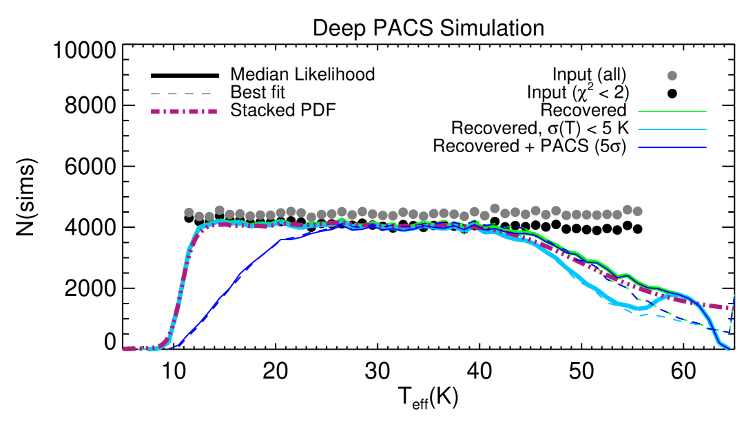
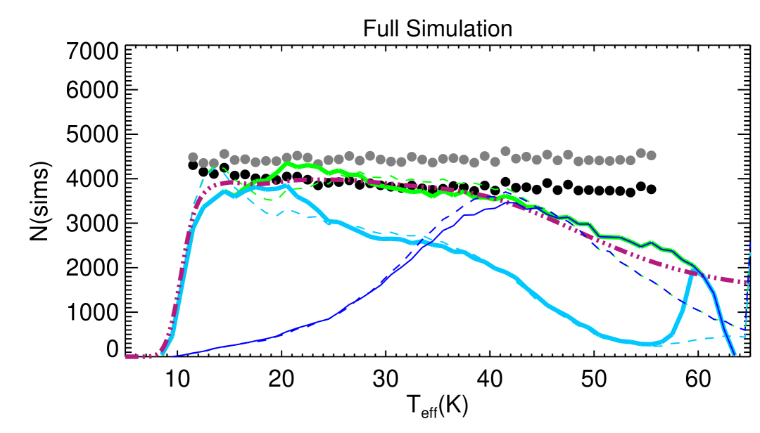
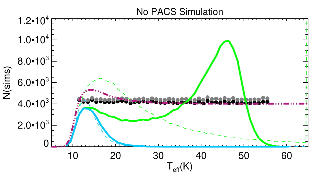
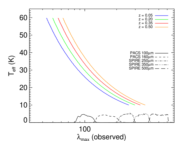
Unsurprisingly, it is clear from comparing the histograms in figure 13 (a) and (b), as well the corresponding contour plots in figure 14, that more sensitive PACS data do enable more precise recovery of the input values of $T_{\mathrm{eff}}$ than we have been able to do in H-ATLAS, reflected by the good agreement between the black and green histogram symbols in figure 13, and by the smaller deviations from the green lines in the $T_{\mathrm{eff}}$ and $L_{\mathrm{dust}}$ contour plots (figure 14) using the more sensitive PACS data than in the H-ATLAS-like simulation. The systematic differences between the input and recovered histograms in figure 13 do not necessarily imply systematic bias between the input and output values. The relatively large random errors on the recovered temperatures for $T>45$ K mean that the recovered histogram in figure 13 (a) smooths over the sharp upper limit on our flat input temperature distribution. In fact, figure 14 (a) shows that the recovered temperatures match the input values very well, despite the peak of the far-IR SED at these temperatures (the strongest spectral feature in our broad-band far-infrared photometry) being at wavelengths shorter than those sampled by the PACS 100 $\mu$m response curve. To demonstrate this, we show the variation between the wavelength of the peak in a model dust SED ($\lambda_{\mathrm{peak}}$) and its isothermal temperature, along with the observed frame PACS and SPIRE response functions for a representative range of redshifts and $\beta=1.82$ in figure 15.

(a) “Deep PACS” simulation

(b) “H-ATLAS-like” simulation

(c) “No PACS” simulation

Figure 14: The results of comparing the input and output values for temperature and dust luminosity in our fixed $\beta=1.82$, “Deep PACS” (a), “H-ATLAS-like” (b) and “no PACS” (c) simulations, from left to right. The top row shows the median-likelihood values for each parameter, while the bottom row shows the best-fit values, with the thick black contours indicating the regions that bound 68.3, 95.5 and 99.7 per cent of the full set of simulated sources, and the thin red contours showing the same percentiles for the $\geq 5\sigma$ PACS-detected fraction of sources. The dashed green lines indicate equal input and output values, while the grey dashed lines in the temperature plots indicate the bounds of the input and output prior distribution; $11<T_{\mathrm{eff}}<56$ K and $5<T_{\mathrm{eff}}<65$ K, respectively.

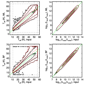
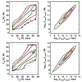
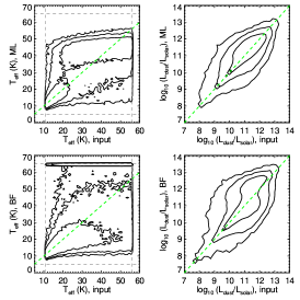
Perhaps more surprisingly, in figures 13 (b) and the left-hand panel of 14 (b) we show how well we may recover $T_{\mathrm{eff}}$ using the comparatively less sensitive PACS data from H-ATLAS (though the simulated SPIRE sensitivities are identical in the two simulations). At $T_{\mathrm{eff}}\ \mbox{{\raisebox{-1.72218pt}{$\stackrel{{\scriptstyle<}}{{{\scriptstyle\sim}}}$} }}20$ K the peak of the SED falls in the SPIRE 250 $\mu$m band (at least for the local galaxies being discussed here) and though there is larger uncertainty due to the absence of high-significance PACS detections for the majority of sources – reflected by the increased spread in the red and black contours in figure 14 (b) relative to the “deep PACS” plot, figure 14 (a) – there is little or no bias toward higher or lower temperatures.

In terms of our ability to recover the input dust luminosity, the right-hand panels of figure 14 (b) indicate that the standard deviation of $(L_{\mathrm{dust}}\ -L_{\mathrm{dust}}^{\mathrm{true}})\approx 0.19$ dex across the full range of $L_{\mathrm{dust}}$ is not dissimilar to the value obtained using the more sensitive PACS simulation shown in figure 14 (a), $\sim$0.14 dex.

Figure 15: The relationship between the wavelength of the peak in the dust SED and the modified black-body-equivalent temperature for redshifts spanning our sample ($z=0.05,0.20,0.35$ and 0.50), assuming $\beta=1.82$. The PACS (100 and 160 $\mu$m) and SPIRE (250, 350 & 500 $\mu$m), response curves are overlaid for the purposes of comparison.

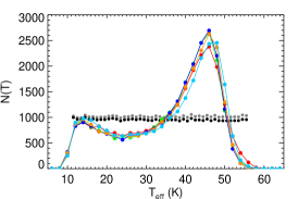
Whilst for the “deep-PACS” and “H-ATLAS-like” simulations there is little to choose between the median-likelihood and best-fit estimates of temperature/luminosity (solid/dashed lines in figure 13, or top and bottom rows in figure 14), in the absence of PACS data this is no longer the case. Median-likelihood estimates of $T_{\mathrm{eff}}$ are biased towards values around 45 K, and the best-fit estimates are similarly unreliable, frequently biased towards lower values (dashed lines) or falling on the upper bound of the temperature prior. The flat stacked temperature PDF for these galaxies at $T_{\mathrm{eff}}\mbox{{\raisebox{-1.72218pt}{$\stackrel{{\scriptstyle>}}{{{\scriptstyle\sim}}}$} }}20$ K, shown as the purple dot-dot-dashed line in figure 13 (c), combined with the large peak in the median-likelihood values around $T_{\mathrm{eff}}\approx 45$ K, reflect the weakness of our temperature constraints in the absence of PACS data.

The severity of the temperature bias in the absence of PACS data is even more apparent in the figure 14 (c), and though the ratio of median-likelihood $L_{\mathrm{dust}}$ to $L_{\mathrm{dust}}^{\mathrm{true}}$ is still centred about unity, the RMS uncertainty is now $\sim$0.5 dex. The best-fit values for $L_{\mathrm{dust}}$ in the absence of PACS data are frequently biased high at the highest luminosities, due to the best-fit temperatures falling on the hot bounds of the prior. It is possible that this situation may improved upon using more information (e.g. an energy balance fitting method; Burgarella et al., 2005; da Cunha et al., 2008; Smith et al., 2012), or assuming a standard temperature for those galaxies with best-fit temperatures falling at the upper bound of the prior, but the contrast between the results derived when including and neglecting the PACS data emphasizes their importance for recovering dust temperatures and luminosities when fitting a simple modified black-body model, even though sources may not be formally significantly detected (e.g. $>3\sigma$). This result complements the results of Gordon et al. (2010) and Skibba et al. (2011), who highlighted the importance of SPIRE data for determining the temperature of the coldest dust; here we stress the importance of both sets of data for determining temperatures across the full range.

5.2 Temperature sensitivity as a function of redshift

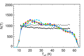
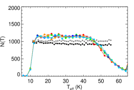
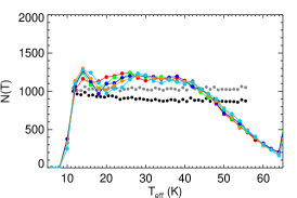
In figure 16 we show histograms of $T_{\mathrm{eff}}$, similar to those in figure 13, but in bins of redshift, such that there are approximately equal numbers of model galaxies in each bin (the bounds of the bins are $z=0.095,0.150,0.210,0.290,0.500$). We show the results for the “deep PACS”, “H-ATLAS-like” and “no PACS” simulations in the left, centre and right-hand columns, respectively, with the median-likelihood values in the top row and the best-fit values in the bottom row. As noted previously, the flat input distribution of temperatures in our simulation enables us to search for fitting bias. In this case, it enables us to see whether our temperature sensitivity varies as a function of redshift due to e.g. the variation in rest-frame wavelengths being sampled. Our simulation is not intended to model the H-ATLAS 250 $\mu$m selection function or the real H-ATLAS coverage of the range in $L_{\mathrm{dust}}-T_{\mathrm{eff}}-z$.

Each histogram has been rescaled in the vertical direction for the purposes of comparison. We overlay the histograms of recovered values in each redshift bin on the flat input distribution (in grey) and on the input distribution of galaxies that have good fits when they are recovered (i.e. reduced $\chi^{2}<2.0$; in black). From comparing the coloured histograms in each simulation, it is clear that there is little - if any - evidence for temperature fitting bias that varies as a function of redshift. Figure 16 also reinforces the idea that there is little difference between the best-fit values and the median-likelihood values in the presence of PACS data. In their absence, the difference is stark, with best-fit values biased towards cold values ($T_{\mathrm{eff}}\approx 16$ K), and median-likelihood values having a peak near 45 K, (though the severity of this bias might be improved with a more physically-motivated choice of temperature prior).

(a) “Deep PACS”, median-likelihood

(b) “H-ATLAS-like”, median-likelihood

(c) “No PACS”, median-likelihood

(d) “Deep PACS”, best-fit

(e) “H-ATLAS-like”, best-fit

(f) “No PACS”, best-fit

Figure 16: The variation in the recovered simulated temperatures assuming $\beta=1.82$ in bins of redshift for all sources in our simulation (i.e. we make no SNR cuts apart from the 250 $\mu$m selection. The left-hand column shows the results for the “Deep PACS” simulation, the central column the “H-ATLAS-like”, and the right-hand column showing the “no PACS” simulation results. The top row shows the median-likelihood values for each simulation, while the bottom row shows the best-fit results. The different coloured histograms correspond to the five different redshift bins in each simulation, each containing approximately equal numbers of sources, with the histograms having been rescaled in the vertical direction for the purposes of comparison. The redshift ranges for each of the five bins are shown in the legend on the bottom-right figure, and are identical in each panel. The grey histogram shows the input values, which have been chosen at random, while the black histogram shows the input temperatures for those sources which are recovered with good fits (i.e. they have a reduced $\chi^{2}<2.0$).

6 Fixed emissivity index properties of galaxies in H-ATLAS

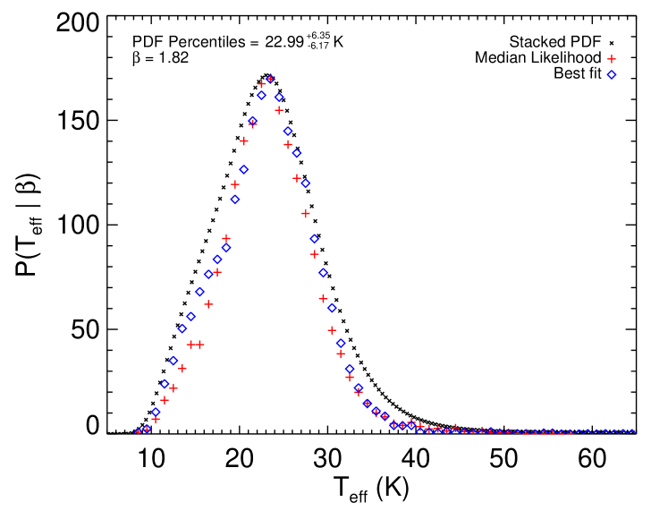
The distributions of $T_{\mathrm{eff}}$ and $L_{\mathrm{dust}}$ for the 13,203 of the 13,826 galaxies with $\chi^{2}$ consistent with the isothermal model are shown in figure 17. Clearly, these results – particularly for the temperature estimates – show strong dependence upon our choice of $\beta$. However, even with fixed $\beta$, the distribution of temperatures in H-ATLAS is broad, with median $23.0\pm 0.1$ K and uncertainty between the $16^{\mathrm{th}}$ and $84^{\mathrm{th}}$ percentiles of $\sim\pm 6.3$ K according to the stacked $T_{\mathrm{eff}}$ PDF (black crosses in figure 17). We also show the median-likelihood and best-fit values, as red crosses and blue diamonds, respectively. Our value of $T_{\mathrm{eff}}\ =23.0\pm 0.1$ K compares well with the $26.1\pm 3.5$ K estimated in Smith et al. 2012 for their “PACS-complete” sample assuming $\beta=1.5$, and with other values in the literature, particularly once the different values of $\beta$ and sample selections used in these studies are taken in to account (e.g. Dye et al. 2010, who derive $23\pm 7$, $21.1\pm 0.8$, and 20.0 K respectively, assuming $\beta=2.0$; Auld et al. 2012, who derive $23\pm 7$, $21.1\pm 0.8$, and 20.0 K respectively, assuming $\beta=2.0$; Davies et al. 2012, who derive $23\pm 7$, $21.1\pm 0.8$, and 20.0 K respectively, assuming $\beta=2.0$).

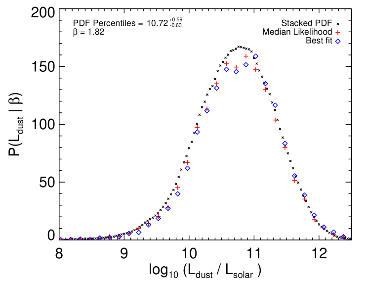
According to the PDF shown in figure 17, the median dust luminosity of a 250 $\mu$m source in H-ATLAS is $\log_{10}(L_{\mathrm{dust}}/L_{\odot})=10.72\pm 0.05$ with an uncertainty of 0.61 dex. Using this stacked PDF, we estimate that while the majority ($\sim 55$ per cent) of H-ATLAS galaxies have far infrared luminosities in the range classified as star forming ($10^{10}<\log_{10}\left(L_{\mathrm{dust}}/L_{\odot}\right)<10^{11}$), a substantial fraction of H-ATLAS galaxies ($\sim 32$ per cent) fall in the Luminous Infrared Galaxy (LIRG) category using our dust SED parametrisation. The rest of the population comprises galaxies in the Normal Infrared Galaxy (NIRG; $\sim$12 per cent of the total) and Ultra-Luminous Infrared Galaxy (ULIRG; $\sim$1 per cent) categories.

Figure 17: Left: The stacked PDF of $\beta=1.82$ isothermal temperature for 250 $\mu$m-selected galaxies in H-ATLAS (black crosses) with the median-likelihood and best-fit estimates overlaid as the red crosses and blue diamonds, respectively. Right: Stacked PDF for $L_{\mathrm{dust}}$ and histogram of median-likelihood and best-fit values in the same colour scheme.

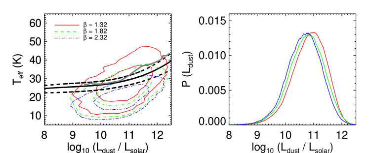
As we mentioned in section 1, it is interesting to probe the relationship between $L_{\mathrm{dust}}$ and $T_{\mathrm{eff}}$ in H-ATLAS galaxies, to study the implications for deriving luminosity or dust-mass functions, for example. The emissivity index has a strong influence on this relationship, as the left hand panel of figure 18 shows. Whilst the implications of the choice of $\beta$ for the derived values of $L_{\mathrm{dust}}$ are comparatively modest (using $\beta=1.32$ or 2.32 – i.e. $\Delta\beta=0.5$ – rather than our fiducial value of $\beta=1.82$ changes our estimates of $L_{\mathrm{dust}}$ by approximately 0.05 dex, as shown in the PDFs in the right panel of figure 18), the impact on the derived values of $T_{\mathrm{eff}}$ is much larger. This is well demonstrated by the difference between the red, green and blue contours in the left-hand panel of figure 18, which represent the results of fitting modified black-body models to the same sample using $\beta=1.32$, 1.82 & 2.32, respectively.

This range of $\beta$ values is perhaps slightly larger than is typically suggested in the literature, but nevertheless it is clear that even at fixed $\beta=1.82$ (our best estimate, derived in section 4.2), the 1 $\sigma$ spread of $T_{\mathrm{eff}}$ values for a given $L_{\mathrm{dust}}$ is likely larger than found by the previously published “L-T” relations in Chapman et al. (2003), Hwang et al. (2010) or Roseboom et al. (2012). The difference is highlighted by the dashed green contours in figure 18, indicating the regions that bound 68.3 and 95.5 percent of the H-ATLAS sources, as compared with the dashed black lines representing the interquartile range of the values obtained in Chapman et al. (2003). Though there is overlap between our $1\,\sigma$ contours and the interquartile-range of Chapman et al. (2003), our results indicate the presence of a larger population of cold galaxies detected by H-ATLAS. As noted by Rahmati & van der Werf (2011), such an increase may be necessary to reproduce the far-IR source counts in the wavelength regime sampled by SPIRE. Though dependent upon the choice of $\beta$, we note that an apparent “L-T”-relation remains irrespective of which value is chosen, albeit with greater spread in temperature for a given luminosity than has been previously noted.

Figure 18: Left: The effects of choosing different values of emissivity index on the derived values of $T_{\mathrm{eff}}$ and $L_{\mathrm{dust}}$ using our simple fixed-$\beta$ SED fitting code on the H-ATLAS phase 1 data set. The distribution of the values derived assuming $\beta=1.32$, 1.82 and 2.32 are shown as the red, green and blue contours respectively, with the best-fit relationships from Chapman et al. (2003) and Hwang et al. (2010) overlaid in black and grey, respectively. The contour levels show the regions enclosed by 68.3 and 95.5 per cent of the data at each value of $\beta$. Right: stacked PDFs of $L_{\mathrm{dust}}$ recovered using the same three values and in the same colour scheme.

7 Conclusions

By using the H-ATLAS phase 1 catalogue over $\sim 161$ deg² (and an ancillary suite of simulations based on H-ATLAS) we show that using simple $\chi^{2}$ SED fitting to recover the intrinsic dust properties of far-infrared sources based on noisy observational data leads to the introduction of an artificial anti-correlation between isothermal temperature and emissivity index, confirming the previous results of Shetty et al. (2009a) and Kelly et al. (2012). The strength of the effect is such that individual estimates of $T_{\mathrm{eff}}$ and $\beta$ are barely correlated with their known input values when $\beta$ is allowed to vary, though we may still derive reasonable estimates of the total dust luminosity between 8-1000 $\mu$m, commonly used as a star formation rate indicator. We have shown that this artificial anti-correlation persists even when using only those objects with the highest significance detections in each of our five far-IR bands, as has been commonly proposed in the literature as a means of mitigating the impact of this degeneracy.

Since a fixed emissivity-index model is likely to remain the standard model for studying far-IR galaxy SEDs for the foreseeable future, we use a simple method to estimate our best estimates of the global mean temperature and emissivity index for galaxies in H-ATLAS. We find that the best values to describe the dust in local ($z<0.5$) sources are $T_{\mathrm{eff}}\ =23.5\pm 0.1$ K and $\beta=1.82\pm 0.02$, where we correct for residual bias in our fitting by making the assumptions that temperature and emissivity index have no intrinsic correlation, and that the intrinsic distribution of values is Gaussian.

By splitting our sample into bins containing approximately equal numbers of sources based on their redshifts, we recover increasing mean temperature for H-ATLAS galaxies as a function of redshift (as expected from previous studies which have found that luminosity and temperature are correlated, though sample selection has also played a role in this correlation; see e.g. Symeonidis et al., 2013, for a comprehensive discussion of selection effects on 60 and 250 $\mu$m-selected surveys). Furthermore, we find tentative evidence, at the 2.8 $\sigma$ level, that the population mean value of the emissivity index positively evolves with redshift, assuming a linear relationship between the two parameters. We leave an investigation of the individual galaxy properties for a future study, since the artificial anti-correlation discussed in section 3 (and noted by other authors, e.g. Shetty et al., 2009a; Kelly et al., 2012; Veneziani et al., 2013) precludes such analysis using these techniques.

It is difficult to reconcile our best-fit results with those of Kelly et al. (2012), who suggest emissivity indices $\beta>2$ for temperatures between $12<T<15$ K, and weak positive correlation between the two (derived using a Spearman’s rank method), though such high values for $\beta$ have been observed by other studies of galactic sources (e.g. Hill et al., 2006; Miyake & Nakagawa, 1993; Kuan et al., 1996) and attributed to grain growth in the central region, or the presence of ice-coated dust grains. Some simple explanations for this apparent discrepancy might be that the dust properties of the Bok globule CB244 may not be representative of the extragalactic population, that any correlation between temperature and emissivity index may be a more complicated function of the dust temperature, that dust emissivity may not simply vary as a power law function of frequency, or some combination of these. Since it is all but certain that the effects of superposing different dust clouds upon a line of sight affect all of these observations (e.g. Shetty et al., 2009a; Veneziani et al., 2013), in this paper we refer to effective temperatures and emissivity indices, which describe the emergent integrated spectrum, and are useful for our purposes. It is likely to be extremely complicated to infer the intrinsic properties of the individual dust populations within these sources using these data.

Based on our best estimate of $\beta_{\mathrm{eff}}$ in H-ATLAS, and on a further suite of ancillary simulations with varying sensitivity in the PACS bands centred on 100 and 160 $\mu$m, we find that our ability to derive fixed-$\beta$ estimates of isothermal temperature and dust luminosity using simple $\chi^{2}$ fitting is dramatically improved by including the H-ATLAS PACS data in our analysis, even though these data are considerably less sensitive than the H-ATLAS SPIRE data, and may not be formally significant detections (e.g. $>3\,\sigma$). We also show that our ability to determine fixed $\beta$ dust temperatures in H-ATLAS shows only weak dependence on the redshift of the galaxy in question, at least out to $z<0.5$.

Finally, we determine that the median $\beta=1.82$ dust luminosity of 250 $\mu$m selected galaxies in H-ATLAS at $z<0.5$ is $\log_{10}(L_{\mathrm{dust}}/L_{\odot})=10.72\pm 0.05$, though the choice of $\beta$ has little influence on this value, including whether it is allowed to vary or is held fixed. We find that while the majority of H-ATLAS galaxies ($\sim 54$ per cent) fall in the star-forming category, a substantial minority ($\sim 31$ per cent) are classified as LIRGs according to their dust luminosity.

References

- Abazajian et al. (2009) Abazajian K. N. et al., 2009, ApJS, 182, 543
- Amblard et al. (2010) Amblard A. et al., 2010, A&A, 518, L9
- Anderson et al. (2010) Anderson L. D. et al., 2010, A&A, 518, L99
- Auld et al. (2012) Auld R. et al., 2012, MNRAS, 191
- Bernard et al. (2010) Bernard J.-P. et al., 2010, A&A, 518, L88
- Blain et al. (2003) Blain A. W., Barnard V. E., Chapman S. C., 2003, MNRAS, 338, 733
- Bonfield et al. (2011) Bonfield D. G. et al., 2011, MNRAS, 416, 13
- Boulanger et al. (1996) Boulanger F., Abergel A., Bernard J.-P., Burton W. B., Desert F.-X., Hartmann D., Lagache G., Puget J.-L., 1996, A&A, 312, 256
- Bracco et al. (2011) Bracco A. et al., 2011, MNRAS, 412, 1151
- Burgarella et al. (2005) Burgarella D., Buat V., Iglesias-Páramo J., 2005, MNRAS, 360, 1413
- Cao Orjales et al. (2012) Cao Orjales J. M. et al., 2012, MNRAS, 427, 1209
- Carilli & Yun (2000) Carilli C. L., Yun M. S., 2000, ApJ, 530, 618
- Casali et al. (2007) Casali M. et al., 2007, A&A, 467, 777
- Chapin et al. (2009) Chapin E. L. et al., 2009, MNRAS, 398, 1793
- Chapman et al. (2003) Chapman S. C., Helou G., Lewis G. F., Dale D. A., 2003, ApJ, 588, 186
- Clements et al. (2010) Clements D. L., Dunne L., Eales S., 2010, MNRAS, 403, 274
- Coppin et al. (2006) Coppin K. et al., 2006, MNRAS, 372, 1621
- Cortese et al. (2012) Cortese L. et al., 2012, A&A, 540, A52
- Coupeaud et al. (2011) Coupeaud A. et al., 2011, A&A, 535, A124
- da Cunha et al. (2008) da Cunha E., Charlot S., Elbaz D., 2008, MNRAS, 388, 1595
- Davies et al. (2012) Davies J. I. et al., 2012, MNRAS, 419, 3505
- Désert et al. (2008) Désert F.-X. et al., 2008, A&A, 481, 411
- Draine & Lee (1984) Draine B. T., Lee H. M., 1984, ApJ, 285, 89
- Driver et al. (2011) Driver S. P. et al., 2011, MNRAS, 413, 971
- Dunne et al. (2000) Dunne L., Eales S., Edmunds M., Ivison R., Alexander P., Clements D. L., 2000, MNRAS, 315, 115
- Dunne & Eales (2001) Dunne L., Eales S. A., 2001, MNRAS, 327, 697
- Dunne et al. (2011) Dunne L. et al., 2011, MNRAS, 417, 1510
- Dupac et al. (2003) Dupac X. et al., 2003, A&A, 404, L11
- Dye et al. (2010) Dye S. et al., 2010, A&A, 518, L10
- Galametz et al. (2012) Galametz M. et al., 2012, MNRAS, 425, 763
- Gordon et al. (2010) Gordon K. D. et al., 2010, A&A, 518, L89
- Griffin et al. (2010) Griffin M. J. et al., 2010, A&A, 518, L3
- Hardcastle et al. (2013) Hardcastle M. J. et al., 2013, MNRAS, 429, 2407
- Hardcastle et al. (2010) Hardcastle M. J. et al., 2010, MNRAS, 409, 122
- Hildebrand (1983) Hildebrand R. H., 1983, QJRAS, 24, 267
- Hill et al. (2006) Hill T., Thompson M. A., Burton M. G., Walsh A. J., Minier V., Cunningham M. R., Pierce-Price D., 2006, MNRAS, 368, 1223
- Hwang et al. (2010) Hwang H. S. et al., 2010, MNRAS, 409, 75
- Ibar et al. (2010) Ibar E. et al., 2010, MNRAS, 409, 38
- Juvela & Ysard (2012) Juvela M., Ysard N., 2012, A&A, 541, A33
- Kelly et al. (2012) Kelly B. C., Shetty R., Stutz A. M., Kauffmann J., Goodman A. A., Launhardt R., 2012, ApJ, 752, 55
- Kennicutt (1998) Kennicutt, Jr. R. C., 1998, ARA&A, 36, 189
- Kovács et al. (2006) Kovács A., Chapman S. C., Dowell C. D., Blain A. W., Ivison R. J., Smail I., Phillips T. G., 2006, ApJ, 650, 592
- Kuan et al. (1996) Kuan Y.-J., Mehringer D. M., Snyder L. E., 1996, ApJ, 459, 619
- Lawrence et al. (2007) Lawrence A. et al., 2007, MNRAS, 379, 1599
- Liang et al. (2012) Liang Z., Fixsen D. J., Gold B., 2012, ArXiv e-prints
- Lutz et al. (2011) Lutz D. et al., 2011, A&A, 532, A90
- Magnelli et al. (2012) Magnelli B. et al., 2012, A&A, 539, A155
- Martínez-Sansigre et al. (2009) Martínez-Sansigre A. et al., 2009, ApJ, 706, 184
- McMahon et al. (1999) McMahon R. G., Priddey R. S., Omont A., Snellen I., Withington S., 1999, MNRAS, 309, L1
- Miyake & Nakagawa (1993) Miyake K., Nakagawa Y., 1993, Icarus, 106, 20
- Nguyen et al. (2010) Nguyen H. T. et al., 2010, A&A, 518, L5
- Oliver et al. (2012) Oliver S. J. et al., 2012, MNRAS, 424, 1614
- Paladini et al. (2012) Paladini R. et al., 2012, ApJ, 760, 149
- Paradis et al. (2010) Paradis D. et al., 2010, A&A, 520, L8
- Pascale et al. (2011) Pascale E. et al., 2011, MNRAS, 415, 911
- Pilbratt et al. (2010) Pilbratt G. L. et al., 2010, A&A, 518, L1
- Planck Collaboration et al. (2011) Planck Collaboration et al., 2011, A&A, 536, A25
- Poglitsch et al. (2010) Poglitsch A. et al., 2010, A&A, 518, L2
- Rahmati & van der Werf (2011) Rahmati A., van der Werf P. P., 2011, MNRAS, 418, 176
- Rigby et al. (2011) Rigby E. E. et al., 2011, MNRAS, 415, 2336
- Roseboom et al. (2013) Roseboom I. G. et al., 2013, ArXiv e-prints
- Roseboom et al. (2012) Roseboom I. G. et al., 2012, MNRAS, 419, 2758
- Rowlands et al. (2012) Rowlands K. et al., 2012, MNRAS, 419, 2545
- Schnee et al. (2010) Schnee S. et al., 2010, ApJ, 708, 127
- Serjeant et al. (2010) Serjeant S. et al., 2010, A&A, 518, L7
- Shetty et al. (2009a) Shetty R., Kauffmann J., Schnee S., Goodman A. A., 2009a, ApJ, 696, 676
- Shetty et al. (2009b) Shetty R., Kauffmann J., Schnee S., Goodman A. A., Ercolano B., 2009b, ApJ, 696, 2234
- Skibba et al. (2011) Skibba R. A. et al., 2011, ApJ, 738, 89
- Smith et al. (2012) Smith D. J. B. et al., 2012, MNRAS, 427, 703
- Smith et al. (2011) Smith D. J. B. et al., 2011, MNRAS, 416, 857
- Smith et al. (2008) Smith D. J. B., Jarvis M. J., Lacy M., Martínez-Sansigre A., 2008, MNRAS, 389, 799
- Smith et al. (2009) Smith D. J. B., Jarvis M. J., Simpson C., Martínez-Sansigre A., 2009, MNRAS, 393, 309
- Smith et al. (2010) Smith D. J. B., Simpson C., Swinbank A. M., Rawlings S., Jarvis M. J., 2010, MNRAS, 404, 1089
- Symeonidis et al. (2013) Symeonidis M. et al., 2013, ArXiv e-prints
- Veneziani et al. (2010) Veneziani M. et al., 2010, ApJ, 713, 959
- Veneziani et al. (2013) Veneziani M., Piacentini F., Noriega-Crespo A., Carey S., Paladini R., Paradis D., 2013, ApJ, 772, 56
- York et al. (2000) York D. G. et al., 2000, AJ, 120, 1579