Optimal Power Allocation for Parameter Tracking in a Distributed Amplify-and-Forward Sensor Network

Feng Jiang, Jie Chen, and A. Lee Swindlehurst
This work was supported by the Air Force Office of Scientific Research grant FA9550-10-1-0310, and by the National Science Foundation under grant CCF-0916073. Center for Pervasive Communications and Computing
University of California at Irvine
Irvine, CA 92697, USA
Email:{feng.jiang, jie.chen, swindle}@uci.edu
Abstract

We consider the problem of optimal power allocation in a sensor network where the sensors observe a dynamic parameter in noise and coherently amplify and forward their observations to a fusion center (FC). The FC uses the observations in a Kalman filter to track the parameter, and we show how to find the optimal gain and phase of the sensor transmissions under both global and individual power constraints in order to minimize the mean squared error (MSE) of the parameter estimate. For the case of a global power constraint, a closed-form solution can be obtained. A numerical optimization is required for individual power constraints, but the problem can be relaxed to a semidefinite programming problem (SDP), and we show that the optimal result can be constructed from the SDP solution. We also study the dual problem of minimizing global and individual power consumption under a constraint on the MSE. As before, a closed-form solution can be found when minimizing total power, while the optimal solution is constructed from the output of an SDP when minimizing the maximum individual sensor power. For purposes of comparison, we derive an exact expression for the outage probability on the MSE for equal-power transmission, which can serve as an upper bound for the case of optimal power control. Finally, we present the results of several simulations to show that the use of optimal power control provides a significant reduction in either MSE or transmit power compared with a non-optimized approach (i.e., equal power transmission).

Index Terms:
Distributed estimation, distributed tracking, wireless sensor networks, amplify-and-forward networks

I Introduction

I-A Background

In a distributed analog amplify-and-forward sensor network, the sensor nodes multiply their noisy observations by a complex factor and transmit the result to a fusion center (FC). In a coherent multiple access channel (MAC), the FC uses the coherent sum of the received signals to estimate the parameter. It has been shown that for Gaussian sensor networks, an analog transmission scheme such as this can achieve the minimum distortion between the source and the recovered signal [1, 2, 3]. The key problem in this setting is designing the multiplication factor for each sensor to meet some goal in terms of estimation accuracy or power consumption. Furthermore, for an optimal solution, these multipliers would have to be updated in scenarios where the parameter or wireless channels are time-varying. In this paper, we focus on tracking a dynamic parameter in a coherent MAC setting.

Most prior work on estimation in distributed amplify-and-forward sensor networks has focused on the situation where the parameter(s) of interest are time-invariant, and either deterministic or i.i.d. Gaussian. The case of an orthogonal MAC, where the FC has access to the individual signals from each sensor, has been studied in [4, 5, 6, 7, 8, 9, 10]. For a coherent MAC, relevant work includes [5, 11, 12, 13, 14, 9]. In [4, 5, 6, 8], two kinds of problems were considered: minimizing the estimation error under sum or individual power constraints, and minimizing the sum transmit power under a constraint on the estimation error. Scaling laws for the estimation error with respect to the number of sensors were derived in [7, 9] under different access schemes and for different power allocation strategies. In [14, 13], the authors exploited a multi-antenna FC to minimize the estimation error.

More relevant to this paper is interesting recent work by Leong et al, who model the (scalar) parameter of interest using a dynamic Gauss-Markov process and assume the FC employs a Kalman filter to track the parameter [15, 16]. In [15], both the orthogonal and coherent MAC were considered and two kinds of optimization problems were formulated: MSE minimization under a global sum transmit power constraint, and sum power minimization problem under an MSE constraint. An asymptotic expression for the MSE outage probability was also derived assuming a large number of sensor nodes. The problem of minimizing the MSE outage probability for the orthogonal MAC with a sum power constraint was studied separately in [16].

I-B Contributions

In this paper, we consider scenarios similar to those in [15]. In particular, we focus on the coherent MAC case assuming a dynamic parameter that is tracked via a Kalman filter at the FC. As detailed in the list of contributions below, we extend the work of [15] for the case of a global sum power constraint, and we go beyond [15] to study problems where either the power of the individual sensors is constrained, or the goal is to minimize the peak power consumption of individual sensors:

  1. 1.

    We find a closed-form expression for the optimal complex transmission gains that minimize the MSE under a constraint on the sum power of all sensor transmissions. While this problem was also solved in [15] using the KKT conditions derived in [5], our approach results in a simpler and more direct solution. We also examine the asymptotic form of the solution for high total transmit power or high noise power at the FC.

  2. 2.

    We find a closed-form expression for the optimal complex transmission gain that minimizes the sum power under a constraint on the MSE. In this case, the expression depends on the eigenvector of a particular matrix. Again, while this problem was also addressed in [15], the numerical solution therein is less direct than the one we obtain. In addition, we find an asymptotic expression for the sum transmit power for a large number of sensors.

  3. 3.

    We show how to find the optimal transmission gains that minimize the MSE under individual sensor power constraints by relaxing the problem to a semi-definite programming (SDP) problem, and then proving that the optimal solution can be constructed from the SDP solution.

  4. 4.

    We show how to find the optimal transmission gains that minimize the maximum individual power over all of the sensors under a constraint on the maximum MSE. Again, we solve the problem using SDP, and then prove that the optimal solution can be constructed from the SDP solution.

  5. 5.

    For the special case where the sensor nodes use equal power transmission, we derive an exact expression for the MSE outage probability.

A subset of the above results were briefly presented in an earlier conference paper [17].

I-C Organization

The rest of the paper is organized as follows. Section II describes the system model for the parameter tracking problem and provides an expression for the MSE obtained at the FC using a standard Kalman filter. Section III investigates the MSE minimization problem under the assumption that the sensor nodes have a sum transmit power constraint. The MSE minimization problem with individual sensor power constraints is formulated and solved in Section III-B. The problems of minimizing the sum power or the maximum individual sensor power with MSE constraints are formulated and optimally solved in Section IV. In Section V, the MSE outage probability for equal power allocation is derived. Numerical results are presented in Section VI and the conclusions are summarized in Section VII.

II System Model

We model the evolution of a complex-valued dynamic parameter θnsubscript𝜃𝑛\theta_{n} using a first-order Gauss-Markov process:

θn=αθn1+un,subscript𝜃𝑛𝛼subscript𝜃𝑛1subscript𝑢𝑛\theta_{n}=\alpha\theta_{n-1}+u_{n}\;,

where n𝑛n denotes the time step, α𝛼\alpha is the correlation parameter and the process noise unsubscript𝑢𝑛u_{n} is zero-mean complex normal with variance σu2superscriptsubscript𝜎𝑢2\sigma_{u}^{2} (denoted by 𝒞𝒩(0,σu2)𝒞𝒩0superscriptsubscript𝜎𝑢2\mathcal{CN}(0,\sigma_{u}^{2})). We assume that θ0subscript𝜃0\theta_{0} is zero mean and that the norm |α|<1𝛼1|\alpha|<1, so that θnsubscript𝜃𝑛\theta_{n} is a stationary process. Thus, the variance of θnsubscript𝜃𝑛\theta_{n} is constant and given by σθ2=σu2/(1|α|2)superscriptsubscript𝜎𝜃2superscriptsubscript𝜎𝑢21superscript𝛼2\sigma_{\theta}^{2}=\sigma_{u}^{2}/\left(1-|\alpha|^{2}\right). A set of N𝑁N sensors measures θnsubscript𝜃𝑛\theta_{n} in the presence of noise; the measurement for the i𝑖ith sensor at time n𝑛n is described by

si,n=θn+vi,n,subscript𝑠𝑖𝑛subscript𝜃𝑛subscript𝑣𝑖𝑛s_{i,n}=\theta_{n}+v_{i,n}\;,

where the measurement noise vi,nsubscript𝑣𝑖𝑛v_{i,n} is distributed as 𝒞𝒩(0,σv,i2)𝒞𝒩0superscriptsubscript𝜎𝑣𝑖2\mathcal{CN}(0,\sigma_{v,i}^{2}). In an amplify-and-forward sensor network, each sensor multiplies its observation by a complex gain factor and transmits the result over a wireless channel to a fusion center (FC). The FC receives a coherent sum of the signals from all N𝑁N sensors in additive noise:

ynsubscript𝑦𝑛\displaystyle y_{n} =\displaystyle= i=1Nhi,nai,nsi,n+wnsuperscriptsubscript𝑖1𝑁subscript𝑖𝑛subscript𝑎𝑖𝑛subscript𝑠𝑖𝑛subscript𝑤𝑛\displaystyle\sum_{i=1}^{N}h_{i,n}a_{i,n}s_{i,n}+w_{n}
=\displaystyle= i=1N(hi,nai,nθn+hi,nai,nvi,n)+wn,superscriptsubscript𝑖1𝑁subscript𝑖𝑛subscript𝑎𝑖𝑛subscript𝜃𝑛subscript𝑖𝑛subscript𝑎𝑖𝑛subscript𝑣𝑖𝑛subscript𝑤𝑛\displaystyle\sum_{i=1}^{N}(h_{i,n}a_{i,n}\theta_{n}+h_{i,n}a_{i,n}v_{i,n})+w_{n}\;,

where hi,nsubscript𝑖𝑛h_{i,n} is the gain of the wireless channel between sensor i𝑖i and the FC, ai,nsubscript𝑎𝑖𝑛a_{i,n} is the complex transmission gain of sensor i𝑖i, and wnsubscript𝑤𝑛w_{n} is noise distributed as 𝒞𝒩(0,σw2)𝒞𝒩0superscriptsubscript𝜎𝑤2\mathcal{CN}(0,\sigma_{w}^{2}). This model can be written more compactly in matrix-vector form, as follows:

yn=𝐚nH𝐡nθn+𝐚nH𝐇n𝐯n+wn,subscript𝑦𝑛superscriptsubscript𝐚𝑛𝐻subscript𝐡𝑛subscript𝜃𝑛superscriptsubscript𝐚𝑛𝐻subscript𝐇𝑛subscript𝐯𝑛subscript𝑤𝑛y_{n}=\mathbf{a}_{n}^{H}\mathbf{h}_{n}\theta_{n}+\mathbf{a}_{n}^{H}\mathbf{H}_{n}\mathbf{v}_{n}+w_{n}\;,

where 𝐡n=[h1,n,,hN,n]Tsubscript𝐡𝑛superscriptsubscript1𝑛subscript𝑁𝑛𝑇\mathbf{h}_{n}=[h_{1,n},\dots,h_{N,n}]^{T}, ()Tsuperscript𝑇(\cdot)^{T} and ()Hsuperscript𝐻(\cdot)^{H} denote the transpose and complex conjugate transpose respectively, 𝐚n=[a1,n,,aN,n]Hsubscript𝐚𝑛superscriptsubscript𝑎1𝑛subscript𝑎𝑁𝑛𝐻\mathbf{a}_{n}=[a_{1,n},\dots,a_{N,n}]^{H} is a vector containing the conjugate of the sensor transmission gains, 𝐇n=diag{h1,n,,hN,n}subscript𝐇𝑛diagsubscript1𝑛subscript𝑁𝑛\mathbf{H}_{n}=\mathrm{diag}\{h_{1,n},\dots,h_{N,n}\} is a diagonal matrix, and the measurement noise vector 𝐯n=[v1,n,,vN,n]Tsubscript𝐯𝑛superscriptsubscript𝑣1𝑛subscript𝑣𝑁𝑛𝑇\mathbf{v}_{n}=[v_{1,n},\dots,v_{N,n}]^{T} has covariance 𝐕=𝔼{𝐯n𝐯nH}=diag{σv,12,,σv,N2}𝐕𝔼subscript𝐯𝑛superscriptsubscript𝐯𝑛𝐻diagsuperscriptsubscript𝜎𝑣12superscriptsubscript𝜎𝑣𝑁2\mathbf{V}=\mathbb{E}\{\mathbf{v}_{n}\mathbf{v}_{n}^{H}\}=\mathrm{diag}\left\{\sigma_{v,1}^{2},\cdots,\sigma_{v,N}^{2}\right\}.

The FC is assumed to know the statistics of the various noise processes, the current channel state 𝐡nsubscript𝐡𝑛\mathbf{h}_{n}, and the transmission gains 𝐚nsubscript𝐚𝑛\mathbf{a}_{n}, and it uses a standard Kalman filter to track the parameter θnsubscript𝜃𝑛\theta_{n} according to the equations below [18]:

  • Prediction Step: θ^n|n1=αθ^n1|n1subscript^𝜃conditional𝑛𝑛1𝛼subscript^𝜃𝑛conditional1𝑛1\hat{\theta}_{n|n-1}=\alpha\hat{\theta}_{n-1|n-1}

  • Prediction MSE: Pn|n1=α2Pn1|n1+σu2subscript𝑃conditional𝑛𝑛1superscript𝛼2subscript𝑃𝑛conditional1𝑛1superscriptsubscript𝜎𝑢2P_{n|n-1}=\alpha^{2}P_{n-1|n-1}+\sigma_{u}^{2}

  • Kalman Gain:

    kn=Pn|n1𝐡nH𝐚n𝐚nH𝐇n𝐕𝐇nH𝐚n+Pn|n1𝐚nH𝐡n𝐡nH𝐚n+σw2subscript𝑘𝑛subscript𝑃conditional𝑛𝑛1superscriptsubscript𝐡𝑛𝐻subscript𝐚𝑛superscriptsubscript𝐚𝑛𝐻subscript𝐇𝑛superscriptsubscript𝐕𝐇𝑛𝐻subscript𝐚𝑛subscript𝑃conditional𝑛𝑛1superscriptsubscript𝐚𝑛𝐻subscript𝐡𝑛superscriptsubscript𝐡𝑛𝐻subscript𝐚𝑛superscriptsubscript𝜎𝑤2k_{n}=\frac{P_{n|n-1}\mathbf{h}_{n}^{H}\mathbf{a}_{n}}{\mathbf{a}_{n}^{H}\mathbf{H}_{n}\mathbf{V}\mathbf{H}_{n}^{H}\mathbf{a}_{n}+P_{n|n-1}\mathbf{a}_{n}^{H}\mathbf{h}_{n}\mathbf{h}_{n}^{H}\mathbf{a}_{n}+\sigma_{w}^{2}}
  • Measurement Update:

    θ^n|n=θ^n|n1+kn(yn𝐚nH𝐡nθ^n|n1)subscript^𝜃conditional𝑛𝑛subscript^𝜃conditional𝑛𝑛1subscript𝑘𝑛subscript𝑦𝑛superscriptsubscript𝐚𝑛𝐻subscript𝐡𝑛subscript^𝜃conditional𝑛𝑛1\hat{\theta}_{n|n}=\hat{\theta}_{n|n-1}+k_{n}\left(y_{n}-\mathbf{a}_{n}^{H}\mathbf{h}_{n}\hat{\theta}_{n|n-1}\right)
  • Filtered MSE:

    Pn|n=(1kn𝐚nH𝐡n)Pn|n1.subscript𝑃conditional𝑛𝑛1subscript𝑘𝑛superscriptsubscript𝐚𝑛𝐻subscript𝐡𝑛subscript𝑃conditional𝑛𝑛1P_{n|n}=(1-k_{n}\mathbf{a}_{n}^{H}\mathbf{h}_{n})P_{n|n-1}\;. (1)

The goal is to determine an optimal choice for the gains 𝐚nsubscript𝐚𝑛\mathbf{a}_{n} that minimizes the filtered MSE under a power constraint, or that minimizes the power consumed in transmitting the data to the FC under an MSE constraint. The optimal gains are then fed back to the individual sensors to use at time n𝑛n.

III Minimizing MSE under a Power Constraint

III-A Global Sum Power Constraint

In this section, we briefly consider the problem of minimizing the MSE under the assumption that the sensor nodes have a sum power constraint. As mentioned earlier, this problem has already been studied in [15], but the solution we provide here is simpler and more direct. The optimization problem can be written as

min𝐚𝐧subscriptsubscript𝐚𝐧\displaystyle\min_{\mathbf{a_{n}}} Pn|nsubscript𝑃conditional𝑛𝑛\displaystyle P_{n|n} (2)
s.t.formulae-sequence𝑠𝑡\displaystyle s.t. 𝐚nH𝐃𝐚nPT,superscriptsubscript𝐚𝑛𝐻subscript𝐃𝐚𝑛subscript𝑃𝑇\displaystyle\mathbf{a}_{n}^{H}\mathbf{D}\mathbf{a}_{n}\leq P_{T}\;,

where 𝐚nH𝐃𝐚nsuperscriptsubscript𝐚𝑛𝐻subscript𝐃𝐚𝑛\mathbf{a}_{n}^{H}\mathbf{D}\mathbf{a}_{n} and PTsubscript𝑃𝑇P_{T} respectively represent the actual and total available transmit power, with 𝐃=diag{σθ2+σv,12,,σθ2+σv,N2}𝐃diagsuperscriptsubscript𝜎𝜃2superscriptsubscript𝜎𝑣12superscriptsubscript𝜎𝜃2superscriptsubscript𝜎𝑣𝑁2\mathbf{D}=\textrm{diag}\{\sigma_{\theta}^{2}+\sigma_{v,1}^{2},\cdots,\sigma_{\theta}^{2}+\sigma_{v,N}^{2}\}. From (1), minimizing the MSE Pn|nsubscript𝑃conditional𝑛𝑛P_{n|n} is equivalent to maximizing

kn𝐚nH𝐡n=Pn|n1𝐚nH𝐡n𝐡nH𝐚n𝐚nH𝐇n𝐕𝐇nH𝐚n+Pn|n1𝐚nH𝐡n𝐡nH𝐚n+σw2,subscript𝑘𝑛superscriptsubscript𝐚𝑛𝐻subscript𝐡𝑛subscript𝑃conditional𝑛𝑛1superscriptsubscript𝐚𝑛𝐻subscript𝐡𝑛superscriptsubscript𝐡𝑛𝐻subscript𝐚𝑛superscriptsubscript𝐚𝑛𝐻subscript𝐇𝑛subscriptsuperscript𝐕𝐇𝐻𝑛subscript𝐚𝑛subscript𝑃conditional𝑛𝑛1superscriptsubscript𝐚𝑛𝐻subscript𝐡𝑛superscriptsubscript𝐡𝑛𝐻subscript𝐚𝑛superscriptsubscript𝜎𝑤2\displaystyle k_{n}\mathbf{a}_{n}^{H}\mathbf{h}_{n}=\frac{P_{n|n-1}\mathbf{a}_{n}^{H}\mathbf{h}_{n}\mathbf{h}_{n}^{H}\mathbf{a}_{n}}{\mathbf{a}_{n}^{H}\mathbf{H}_{n}\mathbf{V}\mathbf{H}^{H}_{n}\mathbf{a}_{n}+P_{n|n-1}\mathbf{a}_{n}^{H}\mathbf{h}_{n}\mathbf{h}_{n}^{H}\mathbf{a}_{n}+\sigma_{w}^{2}}\;,

and after a simple manipulation, the optimization problem in (2) is equivalent to

max𝐚nsubscriptsubscript𝐚𝑛\displaystyle\max_{\mathbf{a}_{n}} 𝐚nH𝐡n𝐡nH𝐚n𝐚nH𝐇n𝐕𝐇nH𝐚n+σw2superscriptsubscript𝐚𝑛𝐻subscript𝐡𝑛superscriptsubscript𝐡𝑛𝐻subscript𝐚𝑛superscriptsubscript𝐚𝑛𝐻subscript𝐇𝑛subscriptsuperscript𝐕𝐇𝐻𝑛subscript𝐚𝑛superscriptsubscript𝜎𝑤2\displaystyle\frac{\mathbf{a}_{n}^{H}\mathbf{h}_{n}\mathbf{h}_{n}^{H}\mathbf{a}_{n}}{\mathbf{a}_{n}^{H}\mathbf{H}_{n}\mathbf{V}\mathbf{H}^{H}_{n}\mathbf{a}_{n}+\sigma_{w}^{2}} (3)
s.t.formulae-sequence𝑠𝑡\displaystyle s.t. 𝐚nH𝐃𝐚nPT.superscriptsubscript𝐚𝑛𝐻subscript𝐃𝐚𝑛subscript𝑃𝑇\displaystyle\mathbf{a}_{n}^{H}\mathbf{D}\mathbf{a}_{n}\leq P_{T}\;.

Denote the optimal solution to (3) as 𝐚nsubscriptsuperscript𝐚𝑛\mathbf{a}^{*}_{n}. It is easy to verify that the objective function of (3) is monotonically increasing in the norm of 𝐚nsubscript𝐚𝑛\mathbf{a}_{n}, which implies that at the optimal solution, the sum transmit power constraint should be met with equality 𝐚nH𝐃𝐚n=PTsubscriptsuperscript𝐚absent𝐻𝑛subscriptsuperscript𝐃𝐚𝑛subscript𝑃𝑇\mathbf{a}^{*H}_{n}\mathbf{D}\mathbf{a}^{*}_{n}=P_{T}. Thus (3) becomes a Rayleigh quotient under a quadratic equality constraint. Since the numerator involves a rank-one quadratic term, a simple closed-form solution is possible. If we define 𝐁=𝐇n𝐕𝐇nH+σw2PT𝐃𝐁subscript𝐇𝑛subscriptsuperscript𝐕𝐇𝐻𝑛superscriptsubscript𝜎𝑤2subscript𝑃𝑇𝐃\mathbf{B}=\mathbf{H}_{n}\mathbf{V}\mathbf{H}^{H}_{n}+\frac{\sigma_{w}^{2}}{P_{T}}\mathbf{D}, the optimal solution is given by

𝐚n=PT𝐡nH𝐁1𝐃𝐁1𝐡n𝐁1𝐡n.superscriptsubscript𝐚𝑛subscript𝑃𝑇superscriptsubscript𝐡𝑛𝐻superscript𝐁1superscript𝐃𝐁1subscript𝐡𝑛superscript𝐁1subscript𝐡𝑛\mathbf{a}_{n}^{*}=\sqrt{\frac{P_{T}}{\mathbf{h}_{n}^{H}\mathbf{B}^{-1}\mathbf{D}\mathbf{B}^{-1}\mathbf{h}_{n}}}\mathbf{B}^{-1}\mathbf{h}_{n}\;. (4)

Note that the phase of each sensor transmission gain is the conjugate of the channel to the FC (recall that 𝐚nsubscript𝐚𝑛\mathbf{a}_{n} contains the conjugate of these transmission gains). In [15], this property was assumed from the beginning in order to get an optimization problem with only real-valued variables; however, we see that this phase-matched solution results even without this assumption.

The maximum value of the objective function in (3) can be expressed as

𝐚nH𝐡n𝐡nH𝐚n𝐚nH(𝐇n𝐕𝐇nH+σw2PT𝐃)𝐚nsuperscriptsubscript𝐚𝑛absent𝐻subscript𝐡𝑛superscriptsubscript𝐡𝑛𝐻superscriptsubscript𝐚𝑛superscriptsubscript𝐚𝑛absent𝐻subscript𝐇𝑛subscriptsuperscript𝐕𝐇𝐻𝑛superscriptsubscript𝜎𝑤2subscript𝑃𝑇𝐃superscriptsubscript𝐚𝑛\displaystyle\frac{\mathbf{a}_{n}^{*H}\mathbf{h}_{n}\mathbf{h}_{n}^{H}\mathbf{a}_{n}^{*}}{\mathbf{a}_{n}^{*H}(\mathbf{H}_{n}\mathbf{V}\mathbf{H}^{H}_{n}+\frac{\sigma_{w}^{2}}{P_{T}}\mathbf{D})\mathbf{a}_{n}^{*}} =\displaystyle= 𝐡nH𝐁1𝐡n.superscriptsubscript𝐡𝑛𝐻superscript𝐁1subscript𝐡𝑛\displaystyle\mathbf{h}_{n}^{H}\mathbf{B}^{-1}\mathbf{h}_{n}\;.

Given that

𝐡nH𝐁1𝐡nsuperscriptsubscript𝐡𝑛𝐻superscript𝐁1subscript𝐡𝑛\displaystyle\mathbf{h}_{n}^{H}\mathbf{B}^{-1}\mathbf{h}_{n} <(a)𝑎\displaystyle\overset{(a)}{<} 𝐡nH(𝐇𝐕𝐇H)1𝐡nsuperscriptsubscript𝐡𝑛𝐻superscriptsuperscript𝐇𝐕𝐇𝐻1subscript𝐡𝑛\displaystyle\mathbf{h}_{n}^{H}(\mathbf{H}\mathbf{V}\mathbf{H}^{H})^{-1}\mathbf{h}_{n} (5)
=\displaystyle= i=1N1σv,i2,superscriptsubscript𝑖1𝑁1superscriptsubscript𝜎𝑣𝑖2\displaystyle\sum_{i=1}^{N}\frac{1}{\sigma_{v,i}^{2}}\;, (6)

where (a)𝑎(a) follows from 𝐁1(𝐇𝐕𝐇H)1precedessuperscript𝐁1superscriptsuperscript𝐇𝐕𝐇𝐻1\mathbf{B}^{-1}\prec(\mathbf{H}\mathbf{V}\mathbf{H}^{H})^{-1}, a lower bound on the MSE can be obtained by plugging (6) into (1):

Pn|nsubscript𝑃conditional𝑛𝑛\displaystyle P_{n|n} >\displaystyle> (111+1(i=1N1σv,i2)Pn|n1)Pn|n11111superscriptsubscript𝑖1𝑁1superscriptsubscript𝜎𝑣𝑖2subscript𝑃conditional𝑛𝑛1subscript𝑃conditional𝑛𝑛1\displaystyle\left(1-\frac{1}{1+\frac{1}{\left(\sum_{i=1}^{N}\frac{1}{\sigma_{v,i}^{2}}\right)P_{n|n-1}}}\right)P_{n|n-1} (7)
=\displaystyle= Pn|n11+(i=1N1σv,i2)Pn|n1.subscript𝑃conditional𝑛𝑛11superscriptsubscript𝑖1𝑁1superscriptsubscript𝜎𝑣𝑖2subscript𝑃conditional𝑛𝑛1\displaystyle\frac{P_{n|n-1}}{1+\left(\sum_{i=1}^{N}\frac{1}{\sigma_{v,i}^{2}}\right)P_{n|n-1}}\;.

Equation (5) becomes an equality when σw2/PT0superscriptsubscript𝜎𝑤2subscript𝑃𝑇0\sigma_{w}^{2}/P_{T}\rightarrow 0 or when the signal-to-noise-ratio (SNR) at the FC is very high, and the resulting optimal sensor transmission gains become

𝐚n=PTi=1N1σv,i4|hn,i|2(σθ2+σv,i2)[1h1,nσv,12,,1hN,nσv,N2]H.superscriptsubscript𝐚𝑛subscript𝑃𝑇superscriptsubscript𝑖1𝑁1superscriptsubscript𝜎𝑣𝑖4superscriptsubscript𝑛𝑖2superscriptsubscript𝜎𝜃2superscriptsubscript𝜎𝑣𝑖2superscript1subscript1𝑛superscriptsubscript𝜎𝑣121subscript𝑁𝑛superscriptsubscript𝜎𝑣𝑁2𝐻\mathbf{a}_{n}^{*}\!=\!\!\sqrt{\frac{P_{T}}{\sum_{i=1}^{N}\frac{1}{\sigma_{v,i}^{4}|h_{n,i}|^{2}(\sigma_{\theta}^{2}+\sigma_{v,i}^{2})}}}\left[\frac{1}{h_{1,n}\sigma_{v,1}^{2}}\;,\cdots\;,\frac{1}{h_{N,n}\sigma_{v,N}^{2}}\right]^{H}\;. (8)

In this case, sensors with small channel gains or low measurement noise are allocated more transmit power. On the other hand, for low SNR at the FC where σw2/PTsuperscriptsubscript𝜎𝑤2subscript𝑃𝑇\sigma_{w}^{2}/P_{T}\rightarrow\infty, we have 𝐁σw2PT𝐃𝐁superscriptsubscript𝜎𝑤2subscript𝑃𝑇𝐃\mathbf{B}\approx\frac{\sigma_{w}^{2}}{P_{T}}\mathbf{D}, and hence from (4) the optimal gain vector is proportional to

𝐚n[h1,nσθ2+σv,12,,hN,nσθ2+σv,N2]H.proportional-tosuperscriptsubscript𝐚𝑛superscriptsubscript1𝑛superscriptsubscript𝜎𝜃2superscriptsubscript𝜎𝑣12subscript𝑁𝑛superscriptsubscript𝜎𝜃2superscriptsubscript𝜎𝑣𝑁2𝐻\mathbf{a}_{n}^{*}\!\propto\!\!\left[\frac{h_{1,n}}{\sigma_{\theta}^{2}+\sigma_{v,1}^{2}}\;,\cdots\;,\frac{h_{N,n}}{\sigma_{\theta}^{2}+\sigma_{v,N}^{2}}\right]^{H}\;. (9)

Interestingly, unlike the high SNR case, for low SNR the sensors with large channel gains are assigned higher power. This observation will be highlighted later in the simulations of Section VI.

III-B Individual Power Constraints

In a distributed sensor network, it is more likely that the power of the individual sensors would be constrained, rather than the total sum power of the network. As seen in the previous section, when the SNR at the FC is high (low), a weak (strong) channel for a given sensor can lead to a high transmission power that the sensor may not be able to support. Thus, in this section we address the problem of minimizing the MSE under individual sensor power constraints, as follows:

min𝐚nsubscriptsubscript𝐚𝑛\displaystyle\min_{\mathbf{a}_{n}} Pn|nsubscript𝑃conditional𝑛𝑛\displaystyle P_{n|n} (10)
s.t.formulae-sequence𝑠𝑡\displaystyle s.t. |ai,n|2(σθ2+σv,i2)PT,i,i=1,,N,formulae-sequencesuperscriptsubscript𝑎𝑖𝑛2superscriptsubscript𝜎𝜃2superscriptsubscript𝜎𝑣𝑖2subscript𝑃𝑇𝑖𝑖1𝑁\displaystyle|a_{i,n}|^{2}(\sigma_{\theta}^{2}+\sigma_{v,i}^{2})\leq P_{T,i}\;,\quad i=1,\cdots,N\;,

where PT,isubscript𝑃𝑇𝑖P_{T,i} is the maximum transmit power available at the i𝑖ith sensor node. Similar to (2), problem (10) can be rewritten as

max𝐚nsubscriptsubscript𝐚𝑛\displaystyle\max_{\mathbf{a}_{n}} 𝐚nH𝐡n𝐡nH𝐚n𝐚nH𝐇n𝐕𝐇nH𝐚n+σw2superscriptsubscript𝐚𝑛𝐻subscript𝐡𝑛superscriptsubscript𝐡𝑛𝐻subscript𝐚𝑛superscriptsubscript𝐚𝑛𝐻subscript𝐇𝑛subscriptsuperscript𝐕𝐇𝐻𝑛subscript𝐚𝑛superscriptsubscript𝜎𝑤2\displaystyle\frac{\mathbf{a}_{n}^{H}\mathbf{h}_{n}\mathbf{h}_{n}^{H}\mathbf{a}_{n}}{\mathbf{a}_{n}^{H}\mathbf{H}_{n}\mathbf{V}\mathbf{H}^{H}_{n}\mathbf{a}_{n}+\sigma_{w}^{2}} (11)
s.t.formulae-sequence𝑠𝑡\displaystyle s.t. |ai,n|2(σθ2+σv,i2)PT,i,i=1,,N.formulae-sequencesuperscriptsubscript𝑎𝑖𝑛2superscriptsubscript𝜎𝜃2superscriptsubscript𝜎𝑣𝑖2subscript𝑃𝑇𝑖𝑖1𝑁\displaystyle|a_{i,n}|^{2}(\sigma_{\theta}^{2}+\sigma_{v,i}^{2})\leq P_{T,i}\;,\quad i=1,\cdots,N\;.

Problem (11) is a quadratically constrained ratio of quadratic functions (QCRQ), and as explained below we will use the approach of [19] to transform the QCRQ problem into a relaxed SDP problem.

Introduce a real auxiliary variable t𝑡t and define 𝐚~n=t𝐚nsubscript~𝐚𝑛𝑡subscript𝐚𝑛\tilde{\mathbf{a}}_{n}=t\mathbf{a}_{n}, so that problem (11) is equivalent to

max𝐚n,tsubscriptsubscript𝐚𝑛𝑡\displaystyle\max_{\mathbf{a}_{n},t} 𝐚~nH𝐡n𝐡nH𝐚~n𝐚~nH𝐇n𝐕𝐇nH𝐚~n+σw2t2superscriptsubscript~𝐚𝑛𝐻subscript𝐡𝑛superscriptsubscript𝐡𝑛𝐻subscript~𝐚𝑛superscriptsubscript~𝐚𝑛𝐻subscript𝐇𝑛subscriptsuperscript𝐕𝐇𝐻𝑛subscript~𝐚𝑛superscriptsubscript𝜎𝑤2superscript𝑡2\displaystyle\frac{\tilde{\mathbf{a}}_{n}^{H}\mathbf{h}_{n}\mathbf{h}_{n}^{H}\tilde{\mathbf{a}}_{n}}{\tilde{\mathbf{a}}_{n}^{H}\mathbf{H}_{n}\mathbf{V}\mathbf{H}^{H}_{n}\tilde{\mathbf{a}}_{n}+\sigma_{w}^{2}t^{2}} (12)
s.t.formulae-sequence𝑠𝑡\displaystyle s.t. 𝐚~nH𝐃i𝐚~nt2PT,i,i=1,,Nformulae-sequencesuperscriptsubscript~𝐚𝑛𝐻subscript𝐃𝑖subscript~𝐚𝑛superscript𝑡2subscript𝑃𝑇𝑖𝑖1𝑁\displaystyle\tilde{\mathbf{a}}_{n}^{H}\mathbf{D}_{i}\tilde{\mathbf{a}}_{n}\leq t^{2}P_{T,i}\;,\quad i=1,\cdots,N
t0,𝑡0\displaystyle t\neq 0\;,

where 𝐃i=diag{0,,0,σθ2+σv,i2,0,,0}subscript𝐃𝑖diag00superscriptsubscript𝜎𝜃2superscriptsubscript𝜎𝑣𝑖200\mathbf{D}_{i}=\textrm{diag}\{0,\cdots,0,\sigma_{\theta}^{2}+\sigma_{v,i}^{2},0,\cdots,0\}. We can further rewrite problem (12) as

max𝐚n,tsubscriptsubscript𝐚𝑛𝑡\displaystyle\max_{\mathbf{a}_{n},t} 𝐚~nH𝐡n𝐡nH𝐚~nsuperscriptsubscript~𝐚𝑛𝐻subscript𝐡𝑛superscriptsubscript𝐡𝑛𝐻subscript~𝐚𝑛\displaystyle\tilde{\mathbf{a}}_{n}^{H}\mathbf{h}_{n}\mathbf{h}_{n}^{H}\tilde{\mathbf{a}}_{n} (13)
s.t.formulae-sequence𝑠𝑡\displaystyle s.t. 𝐚~nH𝐇n𝐕𝐇nH𝐚~n+σw2t2=1superscriptsubscript~𝐚𝑛𝐻subscript𝐇𝑛subscriptsuperscript𝐕𝐇𝐻𝑛subscript~𝐚𝑛superscriptsubscript𝜎𝑤2superscript𝑡21\displaystyle\tilde{\mathbf{a}}_{n}^{H}\mathbf{H}_{n}\mathbf{V}\mathbf{H}^{H}_{n}\tilde{\mathbf{a}}_{n}+\sigma_{w}^{2}t^{2}=1
𝐚~nH𝐃i𝐚~nt2PT,i,i=1,,N.formulae-sequencesuperscriptsubscript~𝐚𝑛𝐻subscript𝐃𝑖subscript~𝐚𝑛superscript𝑡2subscript𝑃𝑇𝑖𝑖1𝑁\displaystyle\tilde{\mathbf{a}}_{n}^{H}\mathbf{D}_{i}\tilde{\mathbf{a}}_{n}\leq t^{2}P_{T,i},\quad i=1,\cdots,N\;.

Note that the constraints in problem (13) already guarantee that t0𝑡0t\neq 0, so this constraint is removed.

Define 𝐚¯n=[𝐚~nHt]Hsubscript¯𝐚𝑛superscriptdelimited-[]subscriptsuperscript~𝐚𝐻𝑛𝑡𝐻\bar{\mathbf{a}}_{n}=[\tilde{\mathbf{a}}^{H}_{n}\;t]^{H} and the matrices

𝐇¯n=[𝐡n𝐡nH0𝟎T𝟎],𝐂¯n=[𝐇n𝐕𝐇nH𝟎𝟎Tσw2],𝐃¯i=[𝐃i𝟎𝟎TPT,i],formulae-sequencesubscript¯𝐇𝑛delimited-[]subscript𝐡𝑛superscriptsubscript𝐡𝑛𝐻0superscript0𝑇0formulae-sequencesubscript¯𝐂𝑛delimited-[]subscript𝐇𝑛subscriptsuperscript𝐕𝐇𝐻𝑛0superscript0𝑇superscriptsubscript𝜎𝑤2subscript¯𝐃𝑖delimited-[]subscript𝐃𝑖0superscript0𝑇subscript𝑃𝑇𝑖\bar{\mathbf{H}}_{n}=\left[\begin{array}[]{cc}\mathbf{h}_{n}\mathbf{h}_{n}^{H}&0\\ \mathbf{0}^{T}&\mathbf{0}\end{array}\right],\qquad\bar{\mathbf{C}}_{n}=\left[\begin{array}[]{cc}\mathbf{H}_{n}\mathbf{V}\mathbf{H}^{H}_{n}&\mathbf{0}\\ \mathbf{0}^{T}&\sigma_{w}^{2}\end{array}\right],\qquad\bar{\mathbf{D}}_{i}=\left[\begin{array}[]{cc}\mathbf{D}_{i}&\mathbf{0}\\ \mathbf{0}^{T}&-P_{T,i}\end{array}\right]\;,

so that problem (13) can be written in the compact form

max𝐚¯nsubscriptsubscript¯𝐚𝑛\displaystyle\max_{\bar{\mathbf{a}}_{n}} 𝐚¯nH𝐇¯n𝐚¯nsuperscriptsubscript¯𝐚𝑛𝐻subscript¯𝐇𝑛subscript¯𝐚𝑛\displaystyle\bar{\mathbf{a}}_{n}^{H}\bar{\mathbf{H}}_{n}\bar{\mathbf{a}}_{n} (14)
s.t.formulae-sequence𝑠𝑡\displaystyle s.t. 𝐚¯nH𝐂¯n𝐚¯n=1superscriptsubscript¯𝐚𝑛𝐻subscript¯𝐂𝑛subscript¯𝐚𝑛1\displaystyle\bar{\mathbf{a}}_{n}^{H}\bar{\mathbf{C}}_{n}\bar{\mathbf{a}}_{n}=1
𝐚¯nH𝐃¯i𝐚¯n0,i=1,,N.formulae-sequencesuperscriptsubscript¯𝐚𝑛𝐻subscript¯𝐃𝑖subscript¯𝐚𝑛0𝑖1𝑁\displaystyle\bar{\mathbf{a}}_{n}^{H}\bar{\mathbf{D}}_{i}\bar{\mathbf{a}}_{n}\leq 0\;,\quad i=1,\cdots,N\;.

Defining the (N+1)×(N+1)𝑁1𝑁1(N+1)\times(N+1) matrix 𝐀¯=𝐚¯n𝐚¯nH¯𝐀subscript¯𝐚𝑛superscriptsubscript¯𝐚𝑛𝐻\bar{\mathbf{A}}=\bar{\mathbf{a}}_{n}\bar{\mathbf{a}}_{n}^{H}, problem (14) is equivalent to

max𝐀¯subscript¯𝐀\displaystyle\max_{\bar{\mathbf{A}}} tr(𝐀¯𝐇¯n)tr¯𝐀subscript¯𝐇𝑛\displaystyle\mathrm{tr}(\bar{\mathbf{A}}\bar{\mathbf{H}}_{n}) (15)
s.t.formulae-sequence𝑠𝑡\displaystyle s.t. tr(𝐀¯𝐂¯n)=1tr¯𝐀subscript¯𝐂𝑛1\displaystyle\mathrm{tr}(\bar{\mathbf{A}}\bar{\mathbf{C}}_{n})=1
tr(𝐀¯𝐃¯i)0,i=1,,Nformulae-sequencetr¯𝐀subscript¯𝐃𝑖0𝑖1𝑁\displaystyle\mathrm{tr}(\bar{\mathbf{A}}\bar{\mathbf{D}}_{i})\leq 0\;,\quad i=1,\cdots,N
rank(𝐀¯)=1rank¯𝐀1\displaystyle\mathrm{rank}(\bar{\mathbf{A}})=1
𝐀¯0.succeeds-or-equals¯𝐀0\displaystyle\bar{\mathbf{A}}\succeq 0\;.

Were it not for the rank constraint, the problem in (15) would be a standard SDP problem and could be solved in polynomial time using (for example) the interior point method. Given the difficulty of handling the rank constraint, we choose to relax it and solve the simpler problem

max𝐀¯subscript¯𝐀\displaystyle\max_{\bar{\mathbf{A}}} tr(𝐀¯𝐇¯n)tr¯𝐀subscript¯𝐇𝑛\displaystyle\mathrm{tr}(\bar{\mathbf{A}}\bar{\mathbf{H}}_{n}) (16)
s.t.formulae-sequence𝑠𝑡\displaystyle s.t. tr(𝐀¯𝐂¯n)=1tr¯𝐀subscript¯𝐂𝑛1\displaystyle\mathrm{tr}(\bar{\mathbf{A}}\bar{\mathbf{C}}_{n})=1
tr(𝐀¯𝐃¯i)0,i=1,,N.formulae-sequencetr¯𝐀subscript¯𝐃𝑖0𝑖1𝑁\displaystyle\mathrm{tr}(\bar{\mathbf{A}}\bar{\mathbf{D}}_{i})\leq 0\;,\quad i=1,\cdots,N\;.
𝐀¯0,succeeds-or-equals¯𝐀0\displaystyle\bar{\mathbf{A}}\succeq 0\;,

which would provide an upper bound on the optimal value of problem (11), and would in general lead to a suboptimal solution for the vector 𝐚nsubscript𝐚𝑛\mathbf{a}_{n} of transmission gains. However, in the following we show that the optimal solution to the original problem in (10) can be constructed from the solution to the relaxed SDP problem in (16). The optimality of a rank-relaxed SDP problem similar to the one we consider here has previously been noted in [20], but for a different problem related to physical layer security. To describe how to find the optimal solution from the rank-relaxed problem in (16), define 𝐀¯superscript¯𝐀\bar{\mathbf{A}}^{*} to be the solution to (16), 𝐀¯l,msubscriptsuperscript¯𝐀𝑙𝑚\bar{\mathbf{A}}^{*}_{l,m} as the (l,m)𝑙𝑚(l,m)th element of 𝐀¯superscript¯𝐀\bar{\mathbf{A}}^{*}, and 𝐀¯Nsuperscriptsubscript¯𝐀𝑁\bar{\mathbf{A}}_{N}^{*} as the N𝑁Nth order leading principal submatrix of 𝐀¯superscript¯𝐀\bar{\mathbf{A}}^{*} formed by deleting the (N+1)𝑁1(N+1)st row and column of 𝐀¯superscript¯𝐀\bar{\mathbf{A}}^{*}. Then the optimal solution can be found via the following theorem.

Theorem 1.

Define the optimal solution to problem (16) as 𝐀¯superscript¯𝐀\bar{\mathbf{A}}^{*}. Then 𝐀¯N=𝐚𝐚Hsubscriptsuperscript¯𝐀𝑁superscript𝐚𝐚𝐻\bar{\mathbf{A}}^{*}_{N}=\mathbf{a}\mathbf{a}^{H} is rank-one and the optimal solution to problem (10) is given by

𝐚n=1𝐀¯N+1,N+1𝐚.subscriptsuperscript𝐚𝑛1superscriptsubscript¯𝐀𝑁1𝑁1𝐚\mathbf{a}^{*}_{n}=\frac{1}{\sqrt{\bar{\mathbf{A}}_{N+1,N+1}^{*}}}\mathbf{a}\;.
Proof:

We first utilize the strong duality between problem (16) and its dual to find properties of the optimal solution 𝐀¯superscript¯𝐀\bar{\mathbf{A}}^{*}. The dual of problem (16) is given by [21]:

minyi,zsubscriptsubscript𝑦𝑖𝑧\displaystyle\min_{y_{i},z} z𝑧\displaystyle z (17)
s.t.formulae-sequence𝑠𝑡\displaystyle s.t. i=1Nyi𝐃¯i+z𝐂¯n𝐇¯n0succeeds-or-equalssuperscriptsubscript𝑖1𝑁subscript𝑦𝑖subscript¯𝐃𝑖𝑧subscript¯𝐂𝑛subscript¯𝐇𝑛0\displaystyle\sum_{i=1}^{N}y_{i}\bar{\mathbf{D}}_{i}+z\bar{\mathbf{C}}_{n}-\bar{\mathbf{H}}_{n}\succeq 0
y1,,yN,z0.subscript𝑦1subscript𝑦𝑁𝑧0\displaystyle y_{1},\dots,y_{N},z\geq 0\;.

It is easy to verify that there exist strictly feasible points for problems (16) and (17). In particular, for (16), we can construct

𝐀¯f=diag{ab,,ab,b},superscript¯𝐀𝑓diag𝑎𝑏𝑎𝑏𝑏\bar{\mathbf{A}}^{f}=\textrm{diag}\{ab,\cdots,ab,b\}\;,

where

0<0absent\displaystyle 0< a<miniPT,iσθ2+σv,i2,𝑎subscript𝑖subscript𝑃𝑇𝑖superscriptsubscript𝜎𝜃2superscriptsubscript𝜎𝑣𝑖2\displaystyle a<\min_{i}\frac{P_{T,i}}{\sigma_{\theta}^{2}+\sigma_{v,i}^{2}}\;,
b=1i=1Na|hn,i|2σv,i2+σw2.𝑏1superscriptsubscript𝑖1𝑁𝑎superscriptsubscript𝑛𝑖2superscriptsubscript𝜎𝑣𝑖2superscriptsubscript𝜎𝑤2\displaystyle b=\frac{1}{\sum_{i=1}^{N}a|h_{n,i}|^{2}\sigma_{v,i}^{2}+\sigma_{w}^{2}}\;.

For (17), we can randomly select yif>0superscriptsubscript𝑦𝑖𝑓0y_{i}^{f}>0, and set zfsuperscript𝑧𝑓z^{f} large enough such that

zf>max{𝐡nH𝐡n+i=1NyifPT,iσw2,𝐡nH𝐡nyif(σθ2+σv,i2)|hn,i|2σv,i2}.superscript𝑧𝑓superscriptsubscript𝐡𝑛𝐻subscript𝐡𝑛superscriptsubscript𝑖1𝑁superscriptsubscript𝑦𝑖𝑓subscript𝑃𝑇𝑖superscriptsubscript𝜎𝑤2superscriptsubscript𝐡𝑛𝐻subscript𝐡𝑛superscriptsubscript𝑦𝑖𝑓superscriptsubscript𝜎𝜃2superscriptsubscript𝜎𝑣𝑖2superscriptsubscript𝑛𝑖2superscriptsubscript𝜎𝑣𝑖2z^{f}\!>\max\left\{\!\frac{\mathbf{h}_{n}^{H}\mathbf{h}_{n}\!+\!\!\sum_{i=1}^{N}y_{i}^{f}P_{T,i}}{\sigma_{w}^{2}},\frac{\mathbf{h}_{n}^{H}\mathbf{h}_{n}\!-\!y_{i}^{f}(\sigma_{\theta}^{2}\!+\!\sigma_{v,i}^{2})}{|h_{n,i}|^{2}\sigma_{v,i}^{2}}\!\right\}\;.

Then, according to Slater’s theorem, strong duality holds between the primal problem (16) and the dual problem (17) and we have the following complementary condition:

tr(𝐀¯𝐆)=0,trsuperscript¯𝐀superscript𝐆0\textrm{tr}(\bar{\mathbf{A}}^{*}\mathbf{G}^{*})=0\;, (18)

where 𝐆=i=1Nyi𝐃¯i+z𝐂¯n𝐇¯nsuperscript𝐆superscriptsubscript𝑖1𝑁superscriptsubscript𝑦𝑖subscript¯𝐃𝑖superscript𝑧subscript¯𝐂𝑛subscript¯𝐇𝑛\mathbf{G}^{*}=\sum_{i=1}^{N}y_{i}^{*}\bar{\mathbf{D}}_{i}+z^{*}\bar{\mathbf{C}}_{n}-\bar{\mathbf{H}}_{n} and yisuperscriptsubscript𝑦𝑖y_{i}^{*} and zsuperscript𝑧z^{*} denote the optimal solution to problem (17). Due to the special structure of 𝐃¯isubscript¯𝐃𝑖\bar{\mathbf{D}}_{i}, 𝐂¯nsubscript¯𝐂𝑛\bar{\mathbf{C}}_{n} and 𝐇¯nsubscript¯𝐇𝑛\bar{\mathbf{H}}_{n}, 𝐆superscript𝐆\mathbf{G}^{*} can be expressed as

𝐆=[𝐆N𝟎𝟎T𝐆N+1,N+1],superscript𝐆delimited-[]subscriptsuperscript𝐆𝑁0superscript0𝑇subscriptsuperscript𝐆𝑁1𝑁1\mathbf{G}^{*}=\left[\begin{array}[]{cc}\mathbf{G}^{*}_{N}&\mathbf{0}\\ \mathbf{0}^{T}&\mathbf{G}^{*}_{N+1,N+1}\end{array}\right]\;,

where 𝐆N=i=1Nyi𝐃i+z𝐇n𝐕𝐇nH𝐡n𝐡nHsubscriptsuperscript𝐆𝑁superscriptsubscript𝑖1𝑁superscriptsubscript𝑦𝑖subscript𝐃𝑖superscript𝑧subscript𝐇𝑛superscriptsubscript𝐕𝐇𝑛𝐻subscript𝐡𝑛superscriptsubscript𝐡𝑛𝐻\mathbf{G}^{*}_{N}=\sum_{i=1}^{N}y_{i}^{*}\mathbf{D}_{i}+z^{*}\mathbf{H}_{n}\mathbf{V}\mathbf{H}_{n}^{H}-\mathbf{h}_{n}\mathbf{h}_{n}^{H} and 𝐆N+1,N+1=zσw2i=1NyiPT,isubscriptsuperscript𝐆𝑁1𝑁1superscript𝑧superscriptsubscript𝜎𝑤2superscriptsubscript𝑖1𝑁superscriptsubscript𝑦𝑖subscript𝑃𝑇𝑖\mathbf{G}^{*}_{N+1,N+1}=z^{*}\sigma_{w}^{2}-\sum_{i=1}^{N}y_{i}^{*}P_{T,i}. Since both 𝐀¯superscript¯𝐀\bar{\mathbf{A}}^{*} and 𝐆superscript𝐆\mathbf{G}^{*} are positive semidefinite, (18) is equivalent to

𝐀¯𝐆=0.superscript¯𝐀superscript𝐆0\bar{\mathbf{A}}^{*}\mathbf{G}^{*}=0\;.

Additionally, with consideration of the structure of 𝐆superscript𝐆\mathbf{G}^{*}, we have

𝐀¯N𝐆N=0.subscriptsuperscript¯𝐀𝑁subscriptsuperscript𝐆𝑁0\bar{\mathbf{A}}^{*}_{N}\mathbf{G}^{*}_{N}=0\;.

Define 𝐕Gsubscript𝐕𝐺\mathbf{V}_{G} as a set of vectors orthogonal to the row space of 𝐆Nsubscriptsuperscript𝐆𝑁\mathbf{G}^{*}_{N}. Then the column vectors of 𝐀¯Nsuperscriptsubscript¯𝐀𝑁\bar{\mathbf{A}}_{N}^{*} must belong to span(𝐕Gsubscript𝐕𝐺\mathbf{V}_{G}) and rank(𝐀¯N)rank(𝐕G)ranksubscriptsuperscript¯𝐀𝑁ranksubscript𝐕𝐺\textrm{rank}(\bar{\mathbf{A}}^{*}_{N})\leq\textrm{rank}(\mathbf{V}_{G}). For any two matrices 𝐌𝐌\mathbf{M} and 𝐍𝐍\mathbf{N}, we have [22] that rank(𝐌+𝐍)|rank(𝐌)rank(𝐍)|rank𝐌𝐍rank𝐌rank𝐍\textrm{rank}(\mathbf{M}+\mathbf{N})\geq|\textrm{rank}(\mathbf{M})-\textrm{rank}(\mathbf{N})|, so

rank(𝐆N)ranksuperscriptsubscript𝐆𝑁\displaystyle\textrm{rank}(\mathbf{G}_{N}^{*})\!\!\! \displaystyle\geq rank(i=1Nyi𝐃i+z𝐇n𝐕𝐇nH)rank(𝐡n𝐡nH)ranksuperscriptsubscript𝑖1𝑁superscriptsubscript𝑦𝑖subscript𝐃𝑖superscript𝑧subscript𝐇𝑛superscriptsubscript𝐕𝐇𝑛𝐻ranksubscript𝐡𝑛superscriptsubscript𝐡𝑛𝐻\displaystyle\!\!\!\textrm{rank}\left(\sum_{i=1}^{N}y_{i}^{*}\mathbf{D}_{i}+z^{*}\mathbf{H}_{n}\mathbf{V}\mathbf{H}_{n}^{H}\right)\!\!-\textrm{rank}(\mathbf{h}_{n}\mathbf{h}_{n}^{H})
=\displaystyle= N1.𝑁1\displaystyle\!\!\!N-1\;.

and

rank(𝐕G)=Nrank(𝐆N)1.ranksubscript𝐕𝐺𝑁ranksuperscriptsubscript𝐆𝑁1\textrm{rank}(\mathbf{V}_{G})=N-\textrm{rank}(\mathbf{G}_{N}^{*})\leq 1\;. (19)

Since tr(𝐀¯𝐇¯)=𝐡nH𝐀¯N𝐡ntrsuperscript¯𝐀¯𝐇superscriptsubscript𝐡𝑛𝐻subscriptsuperscript¯𝐀𝑁subscript𝐡𝑛\text{tr}(\bar{\mathbf{A}}^{*}\bar{\mathbf{H}})=\mathbf{h}_{n}^{H}\bar{\mathbf{A}}^{*}_{N}\mathbf{h}_{n} and tr(𝐀¯𝐇¯)>tr(𝐀¯f𝐇¯)>0trsuperscript¯𝐀¯𝐇trsuperscript¯𝐀𝑓¯𝐇0\text{tr}(\bar{\mathbf{A}}^{*}\bar{\mathbf{H}})>\text{tr}(\bar{\mathbf{A}}^{f}\bar{\mathbf{H}})>0, we have

𝐀¯N0,rank(𝐀¯N)1.formulae-sequencesubscriptsuperscript¯𝐀𝑁0ranksubscriptsuperscript¯𝐀𝑁1\bar{\mathbf{A}}^{*}_{N}\neq 0\;,\qquad\textrm{rank}(\bar{\mathbf{A}}^{*}_{N})\geq 1\;. (20)

Combining (19) and (20) then leads to

rank(𝐀¯N)=1.ranksubscriptsuperscript¯𝐀𝑁1\textrm{rank}(\bar{\mathbf{A}}^{*}_{N})=1\;.

Although at this point we don’t know whether the optimal solution 𝐀¯superscript¯𝐀\bar{\mathbf{A}}^{*} is rank-one, we can construct a rank-one optimal solution based on 𝐀¯superscript¯𝐀\bar{\mathbf{A}}^{*}. Define the rank-one decomposition of 𝐀¯Nsuperscriptsubscript¯𝐀𝑁\bar{\mathbf{A}}_{N}^{*} as 𝐀¯N=𝐚𝐚Hsuperscriptsubscript¯𝐀𝑁superscript𝐚𝐚𝐻\bar{\mathbf{A}}_{N}^{*}=\mathbf{a}\mathbf{a}^{H}, so that the optimal rank-one solution to problem (16) is

𝐀¯=𝐚¯𝐚¯H,superscript¯𝐀superscript¯𝐚superscript¯𝐚absent𝐻\bar{\mathbf{A}}^{{}^{\prime}}=\bar{\mathbf{a}}^{*}\bar{\mathbf{a}}^{*H}, (21)

where 𝐚¯=[𝐚H𝐀¯N+1,N+1]Hsuperscript¯𝐚superscriptdelimited-[]superscript𝐚𝐻superscriptsubscript¯𝐀𝑁1𝑁1𝐻\bar{\mathbf{a}}^{*}=\left[\mathbf{a}^{H}\;\sqrt{\bar{\mathbf{A}}_{N+1,N+1}^{*}}\right]^{H}. It is easy to verify that the rank-one matrix 𝐀¯superscript¯𝐀\bar{\mathbf{A}}^{{}^{\prime}} can achieve the same result for problem (16) as 𝐀¯superscript¯𝐀\bar{\mathbf{A}}^{*}.

Since (11) is equivalent to problem (10) and (15), and (16) is realized from problem (15) by relaxing the rank-one constraint, in general the solution to (16) provides an upper bound on the optimal value achieved by (11). If the optimal solution to (10) is 𝐚nsubscriptsuperscript𝐚𝑛\mathbf{a}^{*}_{n}, then

𝐚nH𝐡n𝐡nH𝐚n𝐚nH𝐇𝐕𝐇H𝐚n+σw2tr(𝐀¯𝐇¯),superscriptsubscript𝐚𝑛absent𝐻subscript𝐡𝑛superscriptsubscript𝐡𝑛𝐻superscriptsubscript𝐚𝑛superscriptsubscript𝐚𝑛absent𝐻superscript𝐇𝐕𝐇𝐻superscriptsubscript𝐚𝑛superscriptsubscript𝜎𝑤2trsuperscript¯𝐀¯𝐇\frac{\mathbf{a}_{n}^{*H}\mathbf{h}_{n}\mathbf{h}_{n}^{H}\mathbf{a}_{n}^{*}}{\mathbf{a}_{n}^{*H}\mathbf{H}\mathbf{V}\mathbf{H}^{H}\mathbf{a}_{n}^{*}+\sigma_{w}^{2}}\leq\textrm{tr}(\bar{\mathbf{A}}^{*}\bar{\mathbf{H}})\;, (22)

where 𝐚nsuperscriptsubscript𝐚𝑛\mathbf{a}_{n}^{*} and 𝐀¯superscript¯𝐀\bar{\mathbf{A}}^{*} are the optimal solutions to problems (10) and (16) respectively. Equality can be achieved in  (22) provided that an optimal rank-one solution exists for (16), and (21) indicates that such a rank-one solution exists. In the following, we will show how to construct 𝐚nsuperscriptsubscript𝐚𝑛\mathbf{a}_{n}^{*} based on 𝐀¯superscript¯𝐀\bar{\mathbf{A}}^{*}. According to problem (16), since tr(𝐀¯𝐂¯n)=1trsuperscript¯𝐀subscript¯𝐂𝑛1\textrm{tr}(\bar{\mathbf{A}}^{*}\bar{\mathbf{C}}_{n})=1 and 𝐀¯0succeeds-or-equals¯𝐀0\bar{\mathbf{A}}\succeq 0, then we have 𝐀¯0superscript¯𝐀0\bar{\mathbf{A}}^{*}\neq 0 and further 𝐀¯N+1,N+1>0subscriptsuperscript¯𝐀𝑁1𝑁10\bar{\mathbf{A}}^{*}_{N+1,N+1}>0. Based on 𝐚¯superscript¯𝐚\bar{\mathbf{a}}^{*}, the optimal solution to (10) is given by

𝐚n=𝐚¯𝐀¯N+1,N+1,subscriptsuperscript𝐚𝑛superscript¯𝐚superscriptsubscript¯𝐀𝑁1𝑁1\mathbf{a}^{*}_{n}=\frac{\bar{\mathbf{a}}^{*}}{\sqrt{\bar{\mathbf{A}}_{N+1,N+1}^{*}}}\;, (23)

and plugging (23) into (22) we have

𝐚nH𝐡n𝐡nH𝐚n𝐚nH𝐇𝐕𝐇H𝐚n+σw2=tr(𝐀¯𝐇¯),superscriptsubscript𝐚𝑛absent𝐻subscript𝐡𝑛superscriptsubscript𝐡𝑛𝐻superscriptsubscript𝐚𝑛superscriptsubscript𝐚𝑛absent𝐻superscript𝐇𝐕𝐇𝐻superscriptsubscript𝐚𝑛superscriptsubscript𝜎𝑤2trsuperscript¯𝐀¯𝐇\frac{\mathbf{a}_{n}^{*H}\mathbf{h}_{n}\mathbf{h}_{n}^{H}\mathbf{a}_{n}^{*}}{\mathbf{a}_{n}^{*H}\mathbf{H}\mathbf{V}\mathbf{H}^{H}\mathbf{a}_{n}^{*}+\sigma_{w}^{2}}=\textrm{tr}(\bar{\mathbf{A}}^{*}\bar{\mathbf{H}})\;,

which verifies the optimality of 𝐚nsubscriptsuperscript𝐚𝑛\mathbf{a}^{*}_{n}. ∎

IV Minimizing Transmit Power under an MSE Constraint

In this section, we consider the converse of the problems investigated in Section III. We first look at the problem addressed in [15], where the goal is to minimize the sum power consumption of all the sensors under the constraint that the MSE is smaller than some threshold. The asymptotic behavior of the solution is then characterized for a large number of sensors, N𝑁N. Next we study the case where the maximum individual transmit power of any given sensor is minimized under the MSE constraint.

IV-A Minimizing Sum Transmit Power

We can express the problem of minimizing the sum transmit power under the constraint that the MSE is smaller than ϵitalic-ϵ\epsilon as follows:

min𝐚nsubscriptsubscript𝐚𝑛\displaystyle\min_{\mathbf{a}_{n}} 𝐚nH𝐃𝐚nsuperscriptsubscript𝐚𝑛𝐻subscript𝐃𝐚𝑛\displaystyle\mathbf{a}_{n}^{H}\mathbf{D}\mathbf{a}_{n} (24)
s.t.formulae-sequence𝑠𝑡\displaystyle s.t. Pn|nϵ.subscript𝑃conditional𝑛𝑛italic-ϵ\displaystyle P_{n|n}\leq\epsilon\;.

To make (24) feasible, according to (1) and (7) the value of ϵitalic-ϵ\epsilon should satisfy

Pn|n11+(i=1N1σv,i2)Pn|n1ϵPn|n1.subscript𝑃conditional𝑛𝑛11superscriptsubscript𝑖1𝑁1superscriptsubscript𝜎𝑣𝑖2subscript𝑃conditional𝑛𝑛1italic-ϵsubscript𝑃conditional𝑛𝑛1\frac{P_{n|n-1}}{1+\left(\sum_{i=1}^{N}\frac{1}{\sigma_{v,i}^{2}}\right)P_{n|n-1}}\leq\epsilon\leq P_{n|n-1}\;. (25)

As discussed earlier, the MSE is monotonically decreasing in the norm of 𝐚nsubscript𝐚𝑛\mathbf{a}_{n}, so it is clear that setting Pn|n=ϵsubscript𝑃conditional𝑛𝑛italic-ϵP_{n|n}=\epsilon results in the minimum possible transmit power, which we refer to as PTsuperscriptsubscript𝑃𝑇P_{T}^{*}. Conceptually, the problem can be solved by finding the value of PTsuperscriptsubscript𝑃𝑇P_{T}^{*} for which Pn|n=ϵsubscript𝑃conditional𝑛𝑛italic-ϵP_{n|n}=\epsilon, and then substituting this value into the solution found in (4):

𝐚n=PT𝐡nH𝐁1𝐃𝐁1𝐡n𝐁1𝐡n.superscriptsubscript𝐚𝑛superscriptsubscript𝑃𝑇superscriptsubscript𝐡𝑛𝐻superscript𝐁1superscript𝐃𝐁1subscript𝐡𝑛superscript𝐁1subscript𝐡𝑛\mathbf{a}_{n}^{*}=\sqrt{\frac{P_{T}^{*}}{\mathbf{h}_{n}^{H}\mathbf{B}^{-1}\mathbf{D}\mathbf{B}^{-1}\mathbf{h}_{n}}}\mathbf{B}^{-1}\mathbf{h}_{n}\;.

Unlike [15], where an unspecified numerical procedure was required to solve this problem, in the following we present a direct “closed-form” solution that finds the result in terms of the eigenvalue and eigenvector of a particular matrix.

Assuming that ϵitalic-ϵ\epsilon satisfies the feasibility constraint of (25), we use (1) and Pn|n=ϵsubscript𝑃conditional𝑛𝑛italic-ϵP_{n|n}=\epsilon to convert (24) to the following form:

min𝐚nsubscriptsubscript𝐚𝑛\displaystyle\min_{\mathbf{a}_{n}} 𝐚nH𝐃𝐚nsuperscriptsubscript𝐚𝑛𝐻subscript𝐃𝐚𝑛\displaystyle\mathbf{a}_{n}^{H}\mathbf{D}\mathbf{a}_{n} (26)
s.t.formulae-sequence𝑠𝑡\displaystyle s.t. 𝐚nH𝐄n𝐚n(Pn|n1ϵ1)σw2,subscriptsuperscript𝐚𝐻𝑛subscript𝐄𝑛subscript𝐚𝑛subscript𝑃conditional𝑛𝑛1italic-ϵ1superscriptsubscript𝜎𝑤2\displaystyle\mathbf{a}^{H}_{n}\mathbf{E}_{n}\mathbf{a}_{n}\geq\left(\frac{P_{n|n-1}}{\epsilon}-1\right)\sigma_{w}^{2}\;,

where 𝐄n=Pn|n1𝐡n𝐡nH(Pn|n1ϵ1)𝐇n𝐕𝐇nHsubscript𝐄𝑛subscript𝑃conditional𝑛𝑛1subscript𝐡𝑛superscriptsubscript𝐡𝑛𝐻subscript𝑃conditional𝑛𝑛1italic-ϵ1subscript𝐇𝑛subscriptsuperscript𝐕𝐇𝐻𝑛\mathbf{E}_{n}=P_{n|n-1}\mathbf{h}_{n}\mathbf{h}_{n}^{H}-\left(\frac{P_{n|n-1}}{\epsilon}-1\right)\mathbf{H}_{n}\mathbf{V}\mathbf{H}^{H}_{n}. It’s obvious that the constraint in problem (26) should be active at the optimal solution and we can rewrite problem (26) as

min𝐚nsubscriptsubscript𝐚𝑛\displaystyle\min_{\mathbf{a}_{n}} 𝐚nH𝐃𝐚n𝐚nH𝐄n𝐚nsuperscriptsubscript𝐚𝑛𝐻subscript𝐃𝐚𝑛subscriptsuperscript𝐚𝐻𝑛subscript𝐄𝑛subscript𝐚𝑛\displaystyle\frac{\mathbf{a}_{n}^{H}\mathbf{D}\mathbf{a}_{n}}{\mathbf{a}^{H}_{n}\mathbf{E}_{n}\mathbf{a}_{n}} (27)
s.t.formulae-sequence𝑠𝑡\displaystyle s.t. 𝐚nH𝐄n𝐚n=(Pn|n1ϵ1)σw2.subscriptsuperscript𝐚𝐻𝑛subscript𝐄𝑛subscript𝐚𝑛subscript𝑃conditional𝑛𝑛1italic-ϵ1superscriptsubscript𝜎𝑤2\displaystyle\mathbf{a}^{H}_{n}\mathbf{E}_{n}\mathbf{a}_{n}=\left(\frac{P_{n|n-1}}{\epsilon}-1\right)\sigma_{w}^{2}\;.

Since both of 𝐚nH𝐃𝐚nsuperscriptsubscript𝐚𝑛𝐻subscript𝐃𝐚𝑛\mathbf{a}_{n}^{H}\mathbf{D}\mathbf{a}_{n} and 𝐚nH𝐄n𝐚nsubscriptsuperscript𝐚𝐻𝑛subscript𝐄𝑛subscript𝐚𝑛\mathbf{a}^{H}_{n}\mathbf{E}_{n}\mathbf{a}_{n} are positive, problem (27) is equivalent to

max𝐚nsubscriptsubscript𝐚𝑛\displaystyle\max_{\mathbf{a}_{n}} 𝐚nH𝐄n𝐚n𝐚nH𝐃𝐚nsubscriptsuperscript𝐚𝐻𝑛subscript𝐄𝑛subscript𝐚𝑛superscriptsubscript𝐚𝑛𝐻subscript𝐃𝐚𝑛\displaystyle\frac{\mathbf{a}^{H}_{n}\mathbf{E}_{n}\mathbf{a}_{n}}{\mathbf{a}_{n}^{H}\mathbf{D}\mathbf{a}_{n}} (28)
s.t.formulae-sequence𝑠𝑡\displaystyle s.t. 𝐚nH𝐄n𝐚n=(Pn|n1ϵ1)σw2.subscriptsuperscript𝐚𝐻𝑛subscript𝐄𝑛subscript𝐚𝑛subscript𝑃conditional𝑛𝑛1italic-ϵ1superscriptsubscript𝜎𝑤2\displaystyle\mathbf{a}^{H}_{n}\mathbf{E}_{n}\mathbf{a}_{n}=\left(\frac{P_{n|n-1}}{\epsilon}-1\right)\sigma_{w}^{2}\;.

Setting 𝐲=𝐃12𝐚n𝐲superscript𝐃12subscript𝐚𝑛\mathbf{y}=\mathbf{D}^{\frac{1}{2}}\mathbf{a}_{n}, problem (28) becomes a Rayleigh quotient maximization:

max𝐲subscript𝐲\displaystyle\max_{\mathbf{y}} 𝐲H𝐃12𝐄n𝐃12𝐲𝐲H𝐲superscript𝐲𝐻superscript𝐃12subscript𝐄𝑛superscript𝐃12𝐲superscript𝐲𝐻𝐲\displaystyle\frac{\mathbf{y}^{H}\mathbf{D}^{-\frac{1}{2}}\mathbf{E}_{n}\mathbf{D}^{-\frac{1}{2}}\mathbf{y}}{\mathbf{y}^{H}\mathbf{y}}
s.t.formulae-sequence𝑠𝑡\displaystyle s.t. 𝐲H𝐃12𝐄n𝐃12𝐲=(Pn|n1ϵ1)σw2,superscript𝐲𝐻superscript𝐃12subscript𝐄𝑛superscript𝐃12𝐲subscript𝑃conditional𝑛𝑛1italic-ϵ1superscriptsubscript𝜎𝑤2\displaystyle\mathbf{y}^{H}\mathbf{D}^{-\frac{1}{2}}\mathbf{E}_{n}\mathbf{D}^{-\frac{1}{2}}\mathbf{y}=\left(\frac{P_{n|n-1}}{\epsilon}-1\right)\sigma_{w}^{2}\;,

whose solution is given by

𝐲=(Pn|n1ϵ1)σw2𝐯1𝐃12𝐄n𝐃12𝐯1𝐯1,superscript𝐲subscript𝑃conditional𝑛𝑛1italic-ϵ1superscriptsubscript𝜎𝑤2subscript𝐯1superscript𝐃12subscript𝐄𝑛superscript𝐃12subscript𝐯1subscript𝐯1\mathbf{y}^{*}=\sqrt{\frac{\left(\frac{P_{n|n-1}}{\epsilon}-1\right)\sigma_{w}^{2}}{\mathbf{v}_{1}\mathbf{D}^{-\frac{1}{2}}\mathbf{E}_{n}\mathbf{D}^{-\frac{1}{2}}\mathbf{v}_{1}}}\mathbf{v}_{1}\;,

where 𝐯1subscript𝐯1\mathbf{v}_{1} denotes the unit-norm eigenvector corresponding to the largest eigenvalue of 𝐃12𝐄n𝐃12superscript𝐃12subscript𝐄𝑛superscript𝐃12\mathbf{D}^{-\frac{1}{2}}\mathbf{E}_{n}\mathbf{D}^{-\frac{1}{2}}. The optimal solution to the original problem in (24) is thus

𝐚n=(Pn|n1ϵ1)σw2𝐯1𝐃12𝐄n𝐃12𝐯1𝐃12𝐯1.superscriptsubscript𝐚𝑛subscript𝑃conditional𝑛𝑛1italic-ϵ1superscriptsubscript𝜎𝑤2subscript𝐯1superscript𝐃12subscript𝐄𝑛superscript𝐃12subscript𝐯1superscript𝐃12subscript𝐯1\mathbf{a}_{n}^{*}=\sqrt{\frac{\left(\frac{P_{n|n-1}}{\epsilon}-1\right)\sigma_{w}^{2}}{\mathbf{v}_{1}\mathbf{D}^{-\frac{1}{2}}\mathbf{E}_{n}\mathbf{D}^{-\frac{1}{2}}\mathbf{v}_{1}}}\mathbf{D}^{-\frac{1}{2}}\mathbf{v}_{1}\;.

The minimum transmit power required to achieve Pn|n=ϵsubscript𝑃conditional𝑛𝑛italic-ϵP_{n|n}=\epsilon can be expressed as

PT=𝐚nH𝐃𝐚n=(Pn|n1ϵ)σw2ϵλmax{𝐃12𝐄n𝐃12},superscriptsubscript𝑃𝑇superscriptsubscript𝐚𝑛absent𝐻superscriptsubscript𝐃𝐚𝑛subscript𝑃conditional𝑛𝑛1italic-ϵsuperscriptsubscript𝜎𝑤2italic-ϵsubscript𝜆superscript𝐃12subscript𝐄𝑛superscript𝐃12P_{T}^{*}=\mathbf{a}_{n}^{*H}\mathbf{D}\mathbf{a}_{n}^{*}=\frac{(P_{n|n-1}-\epsilon)\sigma_{w}^{2}}{\epsilon\lambda_{\max}\{\mathbf{D}^{-\frac{1}{2}}\mathbf{E}_{n}\mathbf{D}^{-\frac{1}{2}}\}}\;, (29)

where λmax()subscript𝜆\lambda_{\max}(\cdot) represents the largest eigenvalue of its matrix argument. A more precise expression for PTsuperscriptsubscript𝑃𝑇P_{T}^{*} can be found when the number of sensors N𝑁N is large, as shown in Theorem 2 below. The theorem assumes that the channel coefficients are described by the following model:

hi,n=h~i,ndiγ,h~i,n𝒞𝒩(0,1),formulae-sequencesubscript𝑖𝑛subscript~𝑖𝑛superscriptsubscript𝑑𝑖𝛾similar-tosubscript~𝑖𝑛𝒞𝒩01h_{i,n}=\frac{\tilde{h}_{i,n}}{d_{i}^{\gamma}},\quad\tilde{h}_{i,n}\sim\mathcal{CN}(0,1)\;, (30)

where disubscript𝑑𝑖d_{i} denotes the distance between sensor i𝑖i and the FC, and γ𝛾\gamma is the propagation path-loss exponent.

Theorem 2.

Assume the channels between the sensors and FC obey the model of (30). When the number of sensors is large, the minimum sum transmit power PTsuperscriptsubscript𝑃𝑇P_{T}^{*} that achieves Pn|n=ϵsubscript𝑃conditional𝑛𝑛italic-ϵP_{n|n}=\epsilon is bounded by

(Pn|n1ϵ)σw2ϵ(Pn|n1𝐡nH𝐃1𝐡nξ)<PT<(Pn|n1ϵ)σw2ϵPn|n1𝐡nH𝐃1𝐡n(1ζ),subscript𝑃conditional𝑛𝑛1italic-ϵsuperscriptsubscript𝜎𝑤2italic-ϵsubscript𝑃conditional𝑛𝑛1superscriptsubscript𝐡𝑛𝐻superscript𝐃1subscript𝐡𝑛𝜉superscriptsubscript𝑃𝑇subscript𝑃conditional𝑛𝑛1italic-ϵsuperscriptsubscript𝜎𝑤2italic-ϵsubscript𝑃conditional𝑛𝑛1superscriptsubscript𝐡𝑛𝐻superscript𝐃1subscript𝐡𝑛1𝜁\frac{\left(P_{n|n-1}-\epsilon\right)\sigma_{w}^{2}}{\epsilon(P_{n|n-1}\mathbf{h}_{n}^{H}\mathbf{D}^{-1}\mathbf{h}_{n}-\xi)}<P_{T}^{*}<\frac{\left(P_{n|n-1}-\epsilon\right)\sigma_{w}^{2}}{\epsilon P_{n|n-1}\mathbf{h}_{n}^{H}\mathbf{D}^{-1}\mathbf{h}_{n}(1-\zeta)}\;,

where random variables ζ𝜁\zeta, ξ𝜉\xi are defined as

ξ𝜉\displaystyle\xi =\displaystyle= (Pn|n1ϵ1)mini{|hi,n|2σv,i2σθ2+σv,i2}subscript𝑃conditional𝑛𝑛1italic-ϵ1subscript𝑖superscriptsubscript𝑖𝑛2superscriptsubscript𝜎𝑣𝑖2superscriptsubscript𝜎𝜃2superscriptsubscript𝜎𝑣𝑖2\displaystyle\left(\frac{P_{n|n-1}}{\epsilon}-1\right)\min_{i}\left\{\frac{|h_{i,n}|^{2}\sigma_{v,i}^{2}}{\sigma_{\theta}^{2}+\sigma_{v,i}^{2}}\right\}
ζ𝜁\displaystyle\zeta =\displaystyle= (Pn|n1ϵ1)maxi{|hi,n|2σv,i2σθ2+σv,i2}Pn|n1𝐡nH𝐃1𝐡n,subscript𝑃conditional𝑛𝑛1italic-ϵ1subscript𝑖superscriptsubscript𝑖𝑛2superscriptsubscript𝜎𝑣𝑖2superscriptsubscript𝜎𝜃2superscriptsubscript𝜎𝑣𝑖2subscript𝑃conditional𝑛𝑛1superscriptsubscript𝐡𝑛𝐻superscript𝐃1subscript𝐡𝑛\displaystyle\frac{\left(\frac{P_{n|n-1}}{\epsilon}-1\right)\max_{i}\left\{\frac{|h_{i,n}|^{2}\sigma_{v,i}^{2}}{\sigma_{\theta}^{2}+\sigma_{v,i}^{2}}\right\}}{P_{n|n-1}\mathbf{h}_{n}^{H}\mathbf{D}^{-1}\mathbf{h}_{n}}\;,

and ζ𝜁\zeta, ξ𝜉\xi converge to 00 in probability.

Proof.

See Appendix A. ∎

According to the above theorem, when N𝑁N\to\infty, the term Pn|n1𝐡nH𝐃1𝐡nsubscript𝑃conditional𝑛𝑛1superscriptsubscript𝐡𝑛𝐻superscript𝐃1subscript𝐡𝑛P_{n|n-1}\mathbf{h}_{n}^{H}\mathbf{D}^{-1}\mathbf{h}_{n} is the dominant factor in the denominator of the bounds on the sum transmit power, and we have the following asymptotic expression

limNPT(Pn|n1ϵ)σw2ϵPn|n1𝐡nH𝐃1𝐡n.similar-to-or-equalssubscript𝑁superscriptsubscript𝑃𝑇subscript𝑃conditional𝑛𝑛1italic-ϵsuperscriptsubscript𝜎𝑤2italic-ϵsubscript𝑃conditional𝑛𝑛1superscriptsubscript𝐡𝑛𝐻superscript𝐃1subscript𝐡𝑛\lim_{N\to\infty}P_{T}^{*}\simeq\frac{(P_{n|n-1}-\epsilon)\sigma_{w}^{2}}{\epsilon P_{n|n-1}\mathbf{h}_{n}^{H}\mathbf{D}^{-1}\mathbf{h}_{n}}\;. (31)

This expression illustrates that to achieve the same MSE, increasing the number of sensors reduces the total required transmit power of the network, as well as the required transmit power per sensor. A similar observation was made in [15]. As shown later, our simulation results show that (31) provides an accurate approximation to (29) as long as ϵitalic-ϵ\epsilon is not too small.

As a final comment on this problem, we note that (24) is equivalent to

min𝐀subscript𝐀\displaystyle\min_{\mathbf{A}} tr(𝐀𝐃)tr𝐀𝐃\displaystyle\textrm{tr}(\mathbf{A}\mathbf{D}) (32)
s.t.formulae-sequence𝑠𝑡\displaystyle s.t. tr(𝐀𝐄n)(Pn|n1ϵ1)σw2trsubscript𝐀𝐄𝑛subscript𝑃conditional𝑛𝑛1italic-ϵ1superscriptsubscript𝜎𝑤2\displaystyle\textrm{tr}(\mathbf{A}\mathbf{E}_{n})\geq\left(\frac{P_{n|n-1}}{\epsilon}-1\right)\sigma_{w}^{2}
rank(𝐀)=1rank𝐀1\displaystyle\mathrm{rank}(\mathbf{A})=1
𝐀0succeeds-or-equals𝐀0\displaystyle\mathbf{A}\succeq 0

for 𝐀=𝐚n𝐚nH𝐀subscript𝐚𝑛superscriptsubscript𝐚𝑛𝐻\mathbf{A}=\mathbf{a}_{n}\mathbf{a}_{n}^{H}. Relaxing the rank-one constraint on 𝐀𝐀\mathbf{A}, problem (32) becomes

min𝐀subscript𝐀\displaystyle\min_{\mathbf{A}} tr(𝐀𝐃)tr𝐀𝐃\displaystyle\textrm{tr}(\mathbf{A}\mathbf{D}) (33)
s.t.formulae-sequence𝑠𝑡\displaystyle s.t. tr(𝐀𝐄n)(Pn|n1ϵ1)σw2,trsubscript𝐀𝐄𝑛subscript𝑃conditional𝑛𝑛1italic-ϵ1superscriptsubscript𝜎𝑤2\displaystyle\textrm{tr}(\mathbf{A}\mathbf{E}_{n})\geq\left(\frac{P_{n|n-1}}{\epsilon}-1\right)\sigma_{w}^{2}\;,
𝐀0.succeeds-or-equals𝐀0\displaystyle\mathbf{A}\succeq 0\;.

Based on the complementary conditions between the dual and primal problems, we can prove that the solution to (33) is rank one, and hence that the relaxed SDP yields the optimal 𝐚nsuperscriptsubscript𝐚𝑛\mathbf{a}_{n}^{*}.

IV-B Minimizing Maximum Individual Transmit Power

Here we focus on the problem of minimizing the maximum transmit power of the individual sensors while attempting to meet an MSE objective:

min𝐚nmaxisubscriptsubscript𝐚𝑛subscript𝑖\displaystyle\min_{\mathbf{a}_{n}}\max_{i} |ai,n|2(σθ2+σv,i2)superscriptsubscript𝑎𝑖𝑛2superscriptsubscript𝜎𝜃2superscriptsubscript𝜎𝑣𝑖2\displaystyle|a_{i,n}|^{2}(\sigma_{\theta}^{2}+\sigma_{v,i}^{2}) (34)
s.t.formulae-sequence𝑠𝑡\displaystyle s.t. Pn|nϵ.subscript𝑃conditional𝑛𝑛italic-ϵ\displaystyle P_{n|n}\leq\epsilon\;.

As in Section III-B, we will convert the problem to a rank-relaxed SDP whose solution nonetheless obeys the rank constraint and hence provides the optimal result. To proceed, introduce an auxiliary variable t𝑡t and rewrite (34) as

min𝐚n,tsubscriptsubscript𝐚𝑛𝑡\displaystyle\min_{\mathbf{a}_{n},t} t𝑡\displaystyle t (35)
s.t.formulae-sequence𝑠𝑡\displaystyle s.t. Pn|nϵsubscript𝑃conditional𝑛𝑛italic-ϵ\displaystyle P_{n|n}\leq\epsilon
|ai,n|2(σθ2+σv,i2)t,i=1,,N.formulae-sequencesuperscriptsubscript𝑎𝑖𝑛2superscriptsubscript𝜎𝜃2superscriptsubscript𝜎𝑣𝑖2𝑡𝑖1𝑁\displaystyle|a_{i,n}|^{2}(\sigma_{\theta}^{2}+\sigma_{v,i}^{2})\leq t,\quad i=1,\cdots,N\;.

Problem (35) is equivalent to

min𝐀,tsubscript𝐀𝑡\displaystyle\min_{\mathbf{A},t} t𝑡\displaystyle t (36)
s.t.formulae-sequence𝑠𝑡\displaystyle s.t. tr(𝐀𝐄n)(Pn|n1ϵ1)σw20trsubscript𝐀𝐄𝑛subscript𝑃conditional𝑛𝑛1italic-ϵ1superscriptsubscript𝜎𝑤20\displaystyle\mathrm{tr}(\mathbf{A}\mathbf{E}_{n})-\left(\frac{P_{n|n-1}}{\epsilon}-1\right)\sigma_{w}^{2}\geq 0
tr(𝐀𝐃i)t0,i=1,,Nformulae-sequencetrsubscript𝐀𝐃𝑖𝑡0𝑖1𝑁\displaystyle\mathrm{tr}(\mathbf{A}\mathbf{D}_{i})-t\leq 0,\;i=1,\cdots,N
𝐀0succeeds-or-equals𝐀0\displaystyle\mathbf{A}\succeq 0
rank(𝐀)=1,rank𝐀1\displaystyle\textrm{rank}\left(\mathbf{A}\right)=1\;,

where 𝐀=𝐚n𝐚nH𝐀subscript𝐚𝑛superscriptsubscript𝐚𝑛𝐻\mathbf{A}=\mathbf{a}_{n}\mathbf{a}_{n}^{H}, 𝐄nsubscript𝐄𝑛\mathbf{E}_{n} is defined as in (26), and 𝐃i=diag{0,,σθ2+σv,i2,0,,0}subscript𝐃𝑖diag0superscriptsubscript𝜎𝜃2superscriptsubscript𝜎𝑣𝑖200\mathbf{D}_{i}=\textrm{diag}\{0,\cdots,\sigma_{\theta}^{2}+\sigma_{v,i}^{2},0,\cdots,0\}, as before.

Relaxing the rank constraint and rewriting the problem to be in standard form, problem (36) becomes

min𝐀~subscript~𝐀\displaystyle\min_{\tilde{\mathbf{A}}} tr(𝐀~𝐓)tr~𝐀𝐓\displaystyle\textrm{tr}(\tilde{\mathbf{A}}\mathbf{T}) (37)
s.t.formulae-sequence𝑠𝑡\displaystyle s.t. tr(𝐀~𝐄~n)(Pn|n1ϵ1)σw20tr~𝐀subscript~𝐄𝑛subscript𝑃conditional𝑛𝑛1italic-ϵ1superscriptsubscript𝜎𝑤20\displaystyle\mathrm{tr}(\tilde{\mathbf{A}}\tilde{\mathbf{E}}_{n})-\left(\frac{P_{n|n-1}}{\epsilon}-1\right)\sigma_{w}^{2}\geq 0
tr(𝐀~𝐅i)0,i=1,,Nformulae-sequencetr~𝐀subscript𝐅𝑖0𝑖1𝑁\displaystyle\mathrm{tr}(\tilde{\mathbf{A}}\mathbf{F}_{i})\leq 0,\quad i=1,\cdots,N
𝐀~0,succeeds-or-equals~𝐀0\displaystyle\tilde{\mathbf{A}}\succeq 0\;,

where

𝐀~=[𝐀𝐰𝐰Ht],𝐓=[𝟎𝟎𝟎1],𝐄~n=[𝐄n𝟎𝟎T0],𝐅i=[𝐃i𝟎𝟎T1],formulae-sequence~𝐀delimited-[]𝐀𝐰superscript𝐰𝐻𝑡formulae-sequence𝐓delimited-[]0001formulae-sequencesubscript~𝐄𝑛delimited-[]subscript𝐄𝑛0superscript0𝑇0subscript𝐅𝑖delimited-[]subscript𝐃𝑖0superscript0𝑇1\tilde{\mathbf{A}}=\left[\begin{array}[]{cc}\mathbf{A}&\mathbf{w}\\ \mathbf{w}^{H}&t\end{array}\right],\qquad\mathbf{T}=\left[\begin{array}[]{cc}\mathbf{0}&\mathbf{0}\\ \mathbf{0}&1\end{array}\right],\qquad\tilde{\mathbf{E}}_{n}=\left[\begin{array}[]{cc}\mathbf{E}_{n}&\mathbf{0}\\ \mathbf{0}^{T}&0\end{array}\right],\qquad\mathbf{F}_{i}=\left[\begin{array}[]{cc}\mathbf{D}_{i}&\mathbf{0}\\ \mathbf{0}^{T}&-1\end{array}\right]\;,

and 𝐰𝐰\mathbf{w} is otherwise arbitrary. Theorem 3 establishes that the optimal solution to (34) can be constructed from the solution to the above relaxed SDP.

Theorem 3.

Define the optimal solution to problem (37) as 𝐀~superscript~𝐀\tilde{\mathbf{A}}^{*}. Then 𝐀~N=𝐚~𝐚~Hsubscriptsuperscript~𝐀𝑁~𝐚superscript~𝐚𝐻\tilde{\mathbf{A}}^{*}_{N}=\tilde{\mathbf{a}}\tilde{\mathbf{a}}^{H} is rank-one and the optimal solution to problem (34) is given by 𝐚n=𝐚~subscriptsuperscript𝐚𝑛~𝐚\mathbf{a}^{*}_{n}=\tilde{\mathbf{a}} .

Proof.

The dual of problem (37) is given by

maxyi,zsubscriptsubscript𝑦𝑖𝑧\displaystyle\max_{y_{i},z} (Pn|n1ϵ1)σw2zsubscript𝑃conditional𝑛𝑛1italic-ϵ1superscriptsubscript𝜎𝑤2𝑧\displaystyle\left(\frac{P_{n|n-1}}{\epsilon}-1\right)\sigma_{w}^{2}z (38)
s.t.formulae-sequence𝑠𝑡\displaystyle s.t. 𝐓+i=1Nyi𝐅iz𝐄~n0succeeds-or-equals𝐓superscriptsubscript𝑖1𝑁subscript𝑦𝑖subscript𝐅𝑖𝑧subscript~𝐄𝑛0\displaystyle\mathbf{T}+\sum_{i=1}^{N}y_{i}\mathbf{F}_{i}-z\tilde{\mathbf{E}}_{n}\succeq 0
y1,,yN,z0.subscript𝑦1subscript𝑦𝑁𝑧0\displaystyle y_{1},\cdots,y_{N},z\geq 0\;.

Using an approach similar to the proof of Theorem 1, one can verify that both (37) and (38) are strictly feasible, and that strong duality holds between the dual problem (38) and the primal problem (37). Based on the complementary conditions, it can be shown that rank(𝐀~N)=1ranksuperscriptsubscript~𝐀𝑁1\text{rank}(\tilde{\mathbf{A}}_{N}^{*})=1. For brevity the details of the proof are omitted. ∎

Similar to problems (2) and (24), duality also exists between (10) and (34). Define the optimal solution to problem (10) as 𝐚nsuperscriptsubscript𝐚𝑛\mathbf{a}_{n}^{*} and the corresponding minimum MSE as Pn|nsuperscriptsubscript𝑃conditional𝑛𝑛P_{n|n}^{*}. If we set ϵ=Pn|nitalic-ϵsuperscriptsubscript𝑃conditional𝑛𝑛\epsilon=P_{n|n}^{*} in (34), the optimal solution is also 𝐚nsuperscriptsubscript𝐚𝑛\mathbf{a}_{n}^{*}.

V MSE Outage Probability for Equal Power Allocation

Here we calculate the MSE outage probability for the suboptimal solution in which each sensor transmits with the same power. The outage probability derived here can serve as an upper bound for the outage performance of the optimal algorithm with individual power constraints. For equal-power transmission, the transmit gain vector is given by

𝐚e=PTN[1σθ2+σv,12,,1(σθ2+σv,N2)]T,subscript𝐚𝑒subscript𝑃𝑇𝑁superscript1superscriptsubscript𝜎𝜃2superscriptsubscript𝜎𝑣121superscriptsubscript𝜎𝜃2superscriptsubscript𝜎𝑣𝑁2𝑇\mathbf{a}_{e}=\sqrt{\frac{P_{T}}{N}}\left[\frac{1}{\sqrt{\sigma_{\theta}^{2}+\sigma_{v,1}^{2}}},\cdots,\frac{1}{\sqrt{(\sigma_{\theta}^{2}+\sigma_{v,N}^{2})}}\right]^{T}\;,

and the corresponding MSE is

Pn|n=(1Pn|n1𝐚eH𝐡n𝐡nH𝐚e𝐚eH𝐇n𝐕𝐇n𝐚e+Pn|n1𝐚eH𝐡n𝐡nH𝐚e+σw2)Pn|n1.subscript𝑃conditional𝑛𝑛1subscript𝑃conditional𝑛𝑛1superscriptsubscript𝐚𝑒𝐻subscript𝐡𝑛superscriptsubscript𝐡𝑛𝐻subscript𝐚𝑒superscriptsubscript𝐚𝑒𝐻subscript𝐇𝑛subscript𝐕𝐇𝑛subscript𝐚𝑒subscript𝑃conditional𝑛𝑛1superscriptsubscript𝐚𝑒𝐻subscript𝐡𝑛superscriptsubscript𝐡𝑛𝐻subscript𝐚𝑒superscriptsubscript𝜎𝑤2subscript𝑃conditional𝑛𝑛1P_{n|n}=\left(1-\frac{P_{n|n-1}\mathbf{a}_{e}^{H}\mathbf{h}_{n}\mathbf{h}_{n}^{H}\mathbf{a}_{e}}{\mathbf{a}_{e}^{H}\mathbf{H}_{n}\mathbf{V}\mathbf{H}_{n}\mathbf{a}_{e}+P_{n|n-1}\mathbf{a}_{e}^{H}\mathbf{h}_{n}\mathbf{h}_{n}^{H}\mathbf{a}_{e}+\sigma_{w}^{2}}\right)P_{n|n-1}\;.

As in Theorem 2, we will assume the Gaussian channel model of (30). The outage probability Pout=Pr{Pn|n>ϵ}subscript𝑃𝑜𝑢𝑡Prsubscript𝑃conditional𝑛𝑛italic-ϵP_{out}=\mathrm{Pr}\left\{P_{n|n}>\epsilon\right\} is evaluated as follows:

Poutsubscript𝑃𝑜𝑢𝑡\displaystyle P_{out} =\displaystyle= Pr{𝐚eH𝐡n𝐡nH𝐚e𝐚eH𝐇𝐕𝐇H𝐚e+σw2<Pn|n1ϵϵPn|n1}Prsuperscriptsubscript𝐚𝑒𝐻subscript𝐡𝑛superscriptsubscript𝐡𝑛𝐻subscript𝐚𝑒superscriptsubscript𝐚𝑒𝐻superscript𝐇𝐕𝐇𝐻subscript𝐚𝑒superscriptsubscript𝜎𝑤2subscript𝑃conditional𝑛𝑛1italic-ϵitalic-ϵsubscript𝑃conditional𝑛𝑛1\displaystyle\mathrm{Pr}\left\{\frac{\mathbf{a}_{e}^{H}\mathbf{h}_{n}\mathbf{h}_{n}^{H}\mathbf{a}_{e}}{\mathbf{a}_{e}^{H}\mathbf{H}\mathbf{V}\mathbf{H}^{H}\mathbf{a}_{e}+\sigma_{w}^{2}}<\frac{P_{n|n-1}-\epsilon}{\epsilon P_{n|n-1}}\right\}
=\displaystyle= Pr{𝐚eH𝐡n𝐡nH𝐚eβ𝐚eH𝐇𝐕𝐇H𝐚e<βσw2}Prsuperscriptsubscript𝐚𝑒𝐻subscript𝐡𝑛superscriptsubscript𝐡𝑛𝐻subscript𝐚𝑒𝛽superscriptsubscript𝐚𝑒𝐻superscript𝐇𝐕𝐇𝐻subscript𝐚𝑒𝛽superscriptsubscript𝜎𝑤2\displaystyle\mathrm{Pr}\left\{\mathbf{a}_{e}^{H}\mathbf{h}_{n}\mathbf{h}_{n}^{H}\mathbf{a}_{e}-\beta\mathbf{a}_{e}^{H}\mathbf{H}\mathbf{V}\mathbf{H}^{H}\mathbf{a}_{e}<\beta\sigma_{w}^{2}\right\}
=\displaystyle= Pr{𝐡~nH(𝐌𝐚~e𝐚~eH𝐌β𝐐)𝐡~nβσw2PT},Prsuperscriptsubscript~𝐡𝑛𝐻𝐌subscript~𝐚𝑒superscriptsubscript~𝐚𝑒𝐻𝐌𝛽𝐐subscript~𝐡𝑛𝛽superscriptsubscript𝜎𝑤2subscript𝑃𝑇\displaystyle\mathrm{Pr}\left\{\tilde{\mathbf{h}}_{n}^{H}\left(\mathbf{M}\tilde{\mathbf{a}}_{e}\tilde{\mathbf{a}}_{e}^{H}\mathbf{M}-\beta\mathbf{Q}\right)\tilde{\mathbf{h}}_{n}\leq\frac{\beta\sigma_{w}^{2}}{P_{T}}\right\}\;,

where

β𝛽\displaystyle\beta =\displaystyle= Pn|n1ϵϵPn|n1,𝐚~e=1PT𝐚e,subscript𝑃conditional𝑛𝑛1italic-ϵitalic-ϵsubscript𝑃conditional𝑛𝑛1subscript~𝐚𝑒1subscript𝑃𝑇subscript𝐚𝑒\displaystyle\frac{P_{n|n-1}-\epsilon}{\epsilon P_{n|n-1}}\;,\;\tilde{\mathbf{a}}_{e}\;=\;\frac{1}{\sqrt{P_{T}}}\mathbf{a}_{e}\;,
𝐌𝐌\displaystyle\mathbf{M} =\displaystyle= diag{1d1α,,1dNα},diag1superscriptsubscript𝑑1𝛼1superscriptsubscript𝑑𝑁𝛼\displaystyle\mathrm{diag}\left\{\frac{1}{d_{1}^{\alpha}},\cdots,\frac{1}{d_{N}^{\alpha}}\right\}\;,
𝐐𝐐\displaystyle\mathbf{Q} =\displaystyle= diag{σv,12N(σθ2+σv,12)d12α,,σv,N2N(σθ2+σv,N2)dN2α},diagsuperscriptsubscript𝜎𝑣12𝑁superscriptsubscript𝜎𝜃2superscriptsubscript𝜎𝑣12superscriptsubscript𝑑12𝛼superscriptsubscript𝜎𝑣𝑁2𝑁superscriptsubscript𝜎𝜃2superscriptsubscript𝜎𝑣𝑁2superscriptsubscript𝑑𝑁2𝛼\displaystyle\mathrm{diag}\left\{\frac{\sigma_{v,1}^{2}}{N(\sigma_{\theta}^{2}+\sigma_{v,1}^{2})d_{1}^{2\alpha}}\;,\cdots,\;\frac{\sigma_{v,N}^{2}}{N(\sigma_{\theta}^{2}+\sigma_{v,N}^{2})d_{N}^{2\alpha}}\right\}\;,
𝐡~nsubscript~𝐡𝑛\displaystyle\tilde{\mathbf{h}}_{n} =\displaystyle= [h~1,n,,h~N,n]T.superscriptsubscript~1𝑛subscript~𝑁𝑛𝑇\displaystyle[\tilde{h}_{1,n}\;,\cdots,\;\tilde{h}_{N,n}]^{T}\;.

If we define 𝐑=𝐌𝐚~e𝐚~eH𝐌β𝐐𝐑𝐌subscript~𝐚𝑒superscriptsubscript~𝐚𝑒𝐻𝐌𝛽𝐐\mathbf{R}=\mathbf{M}\tilde{\mathbf{a}}_{e}\tilde{\mathbf{a}}_{e}^{H}\mathbf{M}-\beta\mathbf{Q}, and label the eigenvalues of 𝐑𝐑\mathbf{R} as λ1,,λNsubscript𝜆1subscript𝜆𝑁\lambda_{1},\cdots,\lambda_{N}, then the random variable 𝐡~nH𝐑𝐡~nsuperscriptsubscript~𝐡𝑛𝐻𝐑subscript~𝐡𝑛\tilde{\mathbf{h}}_{n}^{H}\mathbf{R}\tilde{\mathbf{h}}_{n} can be viewed as the weighted sum of independent chi-squared random variables i=1Nλiχi(2)superscriptsubscript𝑖1𝑁subscript𝜆𝑖subscript𝜒𝑖2\sum_{i=1}^{N}\lambda_{i}\chi_{i}(2). From [23], we have

Pout=1i=1NλiNli(λiλl)1|λi|e(Pn|n1ϵ)σw2ϵPn|n1PTλiu(λi),subscript𝑃𝑜𝑢𝑡1superscriptsubscript𝑖1𝑁superscriptsubscript𝜆𝑖𝑁subscriptproduct𝑙𝑖subscript𝜆𝑖subscript𝜆𝑙1subscript𝜆𝑖superscript𝑒subscript𝑃conditional𝑛𝑛1italic-ϵsuperscriptsubscript𝜎𝑤2italic-ϵsubscript𝑃conditional𝑛𝑛1subscript𝑃𝑇subscript𝜆𝑖𝑢subscript𝜆𝑖P_{out}=1-\sum_{i=1}^{N}\frac{\lambda_{i}^{N}}{\prod_{l\neq i}(\lambda_{i}-\lambda_{l})}\frac{1}{|\lambda_{i}|}e^{-\frac{(P_{n|n-1}-\epsilon)\sigma_{w}^{2}}{\epsilon P_{n|n-1}P_{T}\lambda_{i}}}u(\lambda_{i})\;, (39)

where u()𝑢u(\cdot) is the unit step function. Let e1eNsubscript𝑒1subscript𝑒𝑁e_{1}\geq\cdots\geq e_{N} denote the eigenvalues of 𝐐𝐐\mathbf{Q}, so that from Weyl’s inequality [24] we have the following bounds for the λisubscript𝜆𝑖\lambda_{i}:

𝐚~eH𝐌2𝐚~eβe1superscriptsubscript~𝐚𝑒𝐻superscript𝐌2subscript~𝐚𝑒𝛽subscript𝑒1absent\displaystyle\tilde{\mathbf{a}}_{e}^{H}\mathbf{M}^{2}\tilde{\mathbf{a}}_{e}-\beta e_{1}\leq λ1subscript𝜆1\displaystyle\!\!\!\lambda_{1}\!\!\! 𝐚~eH𝐌2𝐚~eβeN,absentsuperscriptsubscript~𝐚𝑒𝐻superscript𝐌2subscript~𝐚𝑒𝛽subscript𝑒𝑁\displaystyle\leq\tilde{\mathbf{a}}_{e}^{H}\mathbf{M}^{2}\tilde{\mathbf{a}}_{e}-\beta e_{N}\;, (40)
βeNi+1𝛽subscript𝑒𝑁𝑖1absent\displaystyle-\beta e_{N-i+1}\leq λisubscript𝜆𝑖\displaystyle\!\!\!\lambda_{i}\!\!\! βeNi+2,2iN,formulae-sequenceabsent𝛽subscript𝑒𝑁𝑖22𝑖𝑁\displaystyle\leq-\beta e_{N-i+2}\;,\quad 2\leq i\leq N\;, (41)

where 𝐚~eH𝐌2𝐚~e=i=1N1N(σθ2+σv,i2)di2αsuperscriptsubscript~𝐚𝑒𝐻superscript𝐌2subscript~𝐚𝑒superscriptsubscript𝑖1𝑁1𝑁superscriptsubscript𝜎𝜃2superscriptsubscript𝜎𝑣𝑖2superscriptsubscript𝑑𝑖2𝛼\tilde{\mathbf{a}}_{e}^{H}\mathbf{M}^{2}\tilde{\mathbf{a}}_{e}=\sum_{i=1}^{N}\frac{1}{N(\sigma_{\theta}^{2}+\sigma_{v,i}^{2})d_{i}^{2\alpha}} . From (40), when β𝛽\beta is large, λ1subscript𝜆1\lambda_{1} is negative, and when β𝛽\beta is small enough, λ1subscript𝜆1\lambda_{1} is positive. Meanwhile, since all the eigenvalues of 𝐐𝐐\mathbf{Q} is positive, then according to (41) we have that λi<0subscript𝜆𝑖0\lambda_{i}<0 for 2iN2𝑖𝑁2\leq i\leq N. Since only λ1subscript𝜆1\lambda_{1} can be positive, equation (39) can be simplified as

Pout={1λ1N1l1(λ1λl)e(Pn|n1ϵ)σw2ϵPn|n1PTλ1λ1>01λ10.subscript𝑃𝑜𝑢𝑡cases1superscriptsubscript𝜆1𝑁1subscriptproduct𝑙1subscript𝜆1subscript𝜆𝑙superscript𝑒subscript𝑃conditional𝑛𝑛1italic-ϵsuperscriptsubscript𝜎𝑤2italic-ϵsubscript𝑃conditional𝑛𝑛1subscript𝑃𝑇subscript𝜆1subscript𝜆101subscript𝜆10P_{out}=\left\{\begin{array}[]{lr}1-\frac{\lambda_{1}^{N-1}}{\prod_{l\neq 1}(\lambda_{1}-\lambda_{l})}e^{-\frac{(P_{n|n-1}-\epsilon)\sigma_{w}^{2}}{\epsilon P_{n|n-1}P_{T}\lambda_{1}}}&\textrm{$\lambda_{1}>0$}\\ 1&\textrm{$\lambda_{1}\leq 0$}\;.\end{array}\right. (42)

From (42), when the threshold ϵitalic-ϵ\epsilon is too small, β=Pn|n1ϵϵPn|n1𝛽subscript𝑃conditional𝑛𝑛1italic-ϵitalic-ϵsubscript𝑃conditional𝑛𝑛1\beta=\frac{P_{n|n-1}-\epsilon}{\epsilon P_{n|n-1}} will be very large and λ10subscript𝜆10\lambda_{1}\leq 0, then the outage probability Poutsubscript𝑃𝑜𝑢𝑡P_{out} equals 1, which means the MSE Pn|nsubscript𝑃conditional𝑛𝑛P_{n|n} is larger than ϵitalic-ϵ\epsilon for every channel realization 𝐡nsubscript𝐡𝑛\mathbf{h}_{n}. For PTsubscript𝑃𝑇P_{T}\to\infty, the outage probability converges to

Pout={1λ1N1l1(λ1λl)λ1>01λ10.subscript𝑃𝑜𝑢𝑡cases1superscriptsubscript𝜆1𝑁1subscriptproduct𝑙1subscript𝜆1subscript𝜆𝑙subscript𝜆101subscript𝜆10P_{out}=\left\{\begin{array}[]{lr}1-\frac{\lambda_{1}^{N-1}}{\prod_{l\neq 1}(\lambda_{1}-\lambda_{l})}&\textrm{$\lambda_{1}>0$}\\ 1&\textrm{$\lambda_{1}\leq 0$}\;.\end{array}\right.

VI Simulation Results

To investigate the performance of the proposed optimization approaches, the results of several simulation examples are described here. Unless otherwise indicated, the simulations are implemented with the following parameters: distance from the FC to the sensors disubscript𝑑𝑖d_{i} is uniformly distributed over the interval [2,8]28[2,8], path loss exponent is set to γ=1𝛾1\gamma=1, the observation noise power σv,i2superscriptsubscript𝜎𝑣𝑖2\sigma_{v,i}^{2} at the sensors is uniformly distributed over [0,0.5]00.5[0,0.5], the power of the additive noise at the FC is set to σw2=0.5superscriptsubscript𝜎𝑤20.5\sigma_{w}^{2}=0.5, the parameter θ𝜃\theta is assumed to satisfy σθ2=1superscriptsubscript𝜎𝜃21\sigma_{\theta}^{2}=1, and the initial MSE is given by P0|1=0.5subscript𝑃conditional010.5P_{0|-1}=0.5. The MSE shown in the plots is obtained by averaging over 300 realizations of 𝐡nsubscript𝐡𝑛\mathbf{h}_{n}. Two different sum power constraints are considered in the simulations: PT=300subscript𝑃𝑇300P_{T}=300 and PT=3000subscript𝑃𝑇3000P_{T}=3000. To fairly compare the results under sum and individual power constraints, we set PT,i=PTNsubscript𝑃𝑇𝑖subscript𝑃𝑇𝑁P_{T,i}=\frac{P_{T}}{N}, which means that all sensors have the same maximum power when individual constraints are imposed.

Fig. 1 plots the MSE as a function of the number of sensors in the network for both sum and individual power constraints. The results demonstrate that compared with equal power allocation, the optimized power allocation significantly reduces the MSE; in fact, adding sensors with equal power allocation actually increases the MSE, while the MSE always decreases for the optimal methods. The extra flexibility offered by the global power constraint leads to better performance compared with individual power constraints, but the difference in this case is not large. The lower bound on MSE in (7) is also plotted to indicate the performance that that could be achieved with PTsubscript𝑃𝑇P_{T}\to\infty.

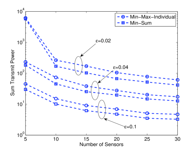
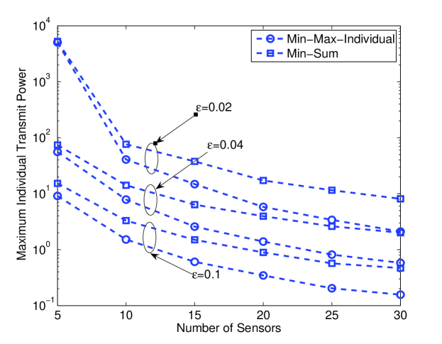
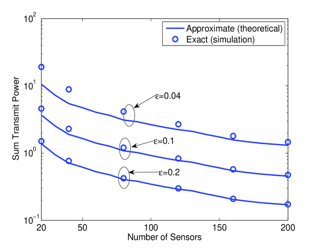
Figs. 2 and 3 respectively examine sum and peak transmit powers required to achieve MSE values of 0.02, 0.04 and 0.1 for varying numbers of sensors. As expected, individual power constraints lead to higher sum power requirements, while sum power constraints result in higher peak power. Interestingly, the individual power constraints lead to roughly a doubling of the required total sum power to achieve the same MSE regardless of the number of sensors, whereas the increase in peak power for the sum constraint relative to individual power constraints grows with N𝑁N, reaching a factor of 4 to 5 on average when N=30𝑁30N=30. Fig. 4 compares the minimum required sum transmit power to achieve various MSE values in (29) with the approximate expression obtained in (31). When ϵ0.1italic-ϵ0.1\epsilon\geq 0.1, the approximation is reasonably good even when N𝑁N is on the order of only 20 to 40. The approximation is less accurate for tighter requirements on ϵitalic-ϵ\epsilon, and requires a larger value of N𝑁N for the approximation to be valid.

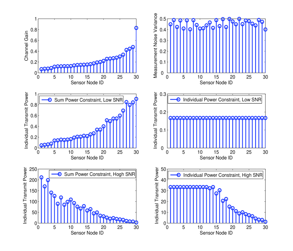
The impact of the SNR at the FC on the sensor power allocation is illustrated in Fig. 5 for a given channel realization and N=30𝑁30N=30 sensors. The x-axis of each plot is ordered according to the channel gain of the sensors, which is shown in the upper left subfigure. The upper right subfigure shows the variance of the measurement noise for each sensor, which for this example was uniformly drawn from the interval [0.4,0.5]0.40.5[0.4,0.5] to better illustrate the effect of the channel gain. The optimal power allocation for this scenario was found assuming both sum and individual power constraints under both low and high SNRs at the FC. The middle subfigures show the power allocation for minimizing MSE assuming a low SNR case with PT=5subscript𝑃𝑇5P_{T}=5, while the bottom subfigures show the allocation for high SNR with PT=1000subscript𝑃𝑇1000P_{T}=1000. Note that, as predicted by (9), the power allocated to the sensors under the sum power constraint for low SNR tends to grow with the channel gain, while as predicted by (8), the allocated power is reduced with increasing sensor gain. The explanation for the different behavior at low and high SNR can be explained as follows: when the SNR is high, the measurement noise will dominate the estimation error at the FC, and the higher the channel gain, the more the measurement noise is amplified, so the sensor nodes with higher channel gains will be allocated less power. When the SNR is low, the additive noise at the FC will dominate the estimation error, the effect of the measurement noise can be neglected, so the nodes with higher channel gains will be allocated more power to increase the power of the desired signal. For individual power constraints, we see that all of the sensors transmit with a maximum power of PT/N=5/30subscript𝑃𝑇𝑁530P_{T}/N=5/30 at low SNR, while at high SNR only the sensors with small channel gains use maximum power (in this case PT/N=1000/30subscript𝑃𝑇𝑁100030P_{T}/N=1000/30), and the power allocated to sensors with large channel gains decreases, as with the sum power constraint.

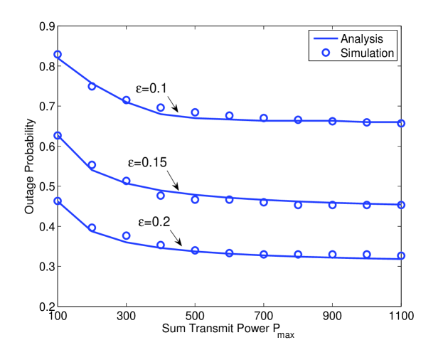
Finally, in Fig. 6, we show that our analytical expression in (42) for the outage probability under equal power allocation closely follows the simulation results for various transmit power levels for a case with N=10𝑁10N=10 sensors. While these outage probabilities represent upper bounds for the optimal (and generally unequal) transmission gains, we note that these bounds are not particularly tight. The outage probabilities achieved by the optimal algorithms are typically much lower than predicted by (42).

VII Conclusion

In this paper, we considered the problem of optimally allocating power in an analog sensor network attempting to track a dynamic parameter via a coherent multiple access channel. We analyzed problems with either constraints on power or constraints on achieved MSE, and we also examined cases involving global sum and individual sensor power constraints. While prior work had been published for minimizing MSE under a sum power constraint and minimizing sum power under an MSE constraint, we were able to derive closed-form solutions that were simpler and more direct. Going beyond the prior work, we derived new asymptotic expressions for the transmission gains that illustrated their limiting behavior for both low and high SNR at the fusion center, and we found a simple expression for the required sum transmit power when the number of sensors is large. Furthermore, we showed how to minimize MSE under individual power constraints, or minimize peak sensor power under MSE constraints, cases that had not been previously considered. In particular, we demonstrated that solutions to these problems could be found by solving a rank-relaxed SDP using standard convex optimization methods. Finally, we derived an exact expression for the MSE outage probability for the special case where the sensors transmit with equal power, and presented a number of simulation results that confirmed our analysis and the performance of the proposed algorithms.

Appendix A Proof of Theorem 2

Proof.

Since 𝐃12𝐄n𝐃12superscript𝐃12subscript𝐄𝑛superscript𝐃12\mathbf{D}^{-\frac{1}{2}}\mathbf{E}_{n}\mathbf{D}^{-\frac{1}{2}} is the sum of a rank-one and a diagonal matrix, we have the following bounds for λmax{𝐃12𝐄n𝐃12}subscript𝜆superscript𝐃12subscript𝐄𝑛superscript𝐃12\lambda_{\max}\{\mathbf{D}^{-\frac{1}{2}}\mathbf{E}_{n}\mathbf{D}^{-\frac{1}{2}}\}:

λmax{𝐃12𝐄n𝐃12}subscript𝜆superscript𝐃12subscript𝐄𝑛superscript𝐃12\displaystyle\lambda_{\max}\{\mathbf{D}^{-\frac{1}{2}}\mathbf{E}_{n}\mathbf{D}^{-\frac{1}{2}}\} <\displaystyle< Pn|n1𝐡nH𝐃1𝐡n(Pn|n1ϵ1)mini{|hi,n|2σv,i2σθ2+σv,i2}subscript𝑃conditional𝑛𝑛1superscriptsubscript𝐡𝑛𝐻superscript𝐃1subscript𝐡𝑛subscript𝑃conditional𝑛𝑛1italic-ϵ1subscript𝑖superscriptsubscript𝑖𝑛2superscriptsubscript𝜎𝑣𝑖2superscriptsubscript𝜎𝜃2superscriptsubscript𝜎𝑣𝑖2\displaystyle P_{n|n-1}\mathbf{h}_{n}^{H}\mathbf{D}^{-1}\mathbf{h}_{n}-\left(\frac{P_{n|n-1}}{\epsilon}-1\right)\min_{i}\left\{\frac{|h_{i,n}|^{2}\sigma_{v,i}^{2}}{\sigma_{\theta}^{2}+\sigma_{v,i}^{2}}\right\} (43)
=\displaystyle= Pn|n1𝐡nH𝐃1𝐡nξ,subscript𝑃conditional𝑛𝑛1superscriptsubscript𝐡𝑛𝐻superscript𝐃1subscript𝐡𝑛𝜉\displaystyle P_{n|n-1}\mathbf{h}_{n}^{H}\mathbf{D}^{-1}\mathbf{h}_{n}-\xi\;,
λmax{𝐃12𝐄n𝐃12}subscript𝜆superscript𝐃12subscript𝐄𝑛superscript𝐃12\displaystyle\lambda_{\max}\{\mathbf{D}^{-\frac{1}{2}}\mathbf{E}_{n}\mathbf{D}^{-\frac{1}{2}}\} >\displaystyle> Pn|n1𝐡nH𝐃1𝐡n(Pn|n1ϵ1)maxi{|hi,n|2σv,i2σθ2+σv,i2}subscript𝑃conditional𝑛𝑛1superscriptsubscript𝐡𝑛𝐻superscript𝐃1subscript𝐡𝑛subscript𝑃conditional𝑛𝑛1italic-ϵ1subscript𝑖superscriptsubscript𝑖𝑛2superscriptsubscript𝜎𝑣𝑖2superscriptsubscript𝜎𝜃2superscriptsubscript𝜎𝑣𝑖2\displaystyle P_{n|n-1}\mathbf{h}_{n}^{H}\mathbf{D}^{-1}\mathbf{h}_{n}-\left(\frac{P_{n|n-1}}{\epsilon}-1\right)\max_{i}\left\{\frac{|h_{i,n}|^{2}\sigma_{v,i}^{2}}{\sigma_{\theta}^{2}+\sigma_{v,i}^{2}}\right\} (44)
=\displaystyle= Pn|n1𝐡nH𝐃1𝐡n(1ζ),subscript𝑃conditional𝑛𝑛1superscriptsubscript𝐡𝑛𝐻superscript𝐃1subscript𝐡𝑛1𝜁\displaystyle P_{n|n-1}\mathbf{h}_{n}^{H}\mathbf{D}^{-1}\mathbf{h}_{n}(1-\zeta)\;,

where we define

ξ𝜉\displaystyle\xi =\displaystyle= (Pn|n1ϵ1)mini{|hi,n|2σv,i2σθ2+σv,i2},subscript𝑃conditional𝑛𝑛1italic-ϵ1subscript𝑖superscriptsubscript𝑖𝑛2superscriptsubscript𝜎𝑣𝑖2superscriptsubscript𝜎𝜃2superscriptsubscript𝜎𝑣𝑖2\displaystyle\left(\frac{P_{n|n-1}}{\epsilon}-1\right)\min_{i}\left\{\frac{|h_{i,n}|^{2}\sigma_{v,i}^{2}}{\sigma_{\theta}^{2}+\sigma_{v,i}^{2}}\right\}\;,
ζ𝜁\displaystyle\zeta =\displaystyle= (Pn|n1ϵ1)maxi{|hi,n|2σv,i2σθ2+σv,i2}Pn|n1𝐡nH𝐃1𝐡n.subscript𝑃conditional𝑛𝑛1italic-ϵ1subscript𝑖superscriptsubscript𝑖𝑛2superscriptsubscript𝜎𝑣𝑖2superscriptsubscript𝜎𝜃2superscriptsubscript𝜎𝑣𝑖2subscript𝑃conditional𝑛𝑛1superscriptsubscript𝐡𝑛𝐻superscript𝐃1subscript𝐡𝑛\displaystyle\frac{\left(\frac{P_{n|n-1}}{\epsilon}-1\right)\max_{i}\left\{\frac{|h_{i,n}|^{2}\sigma_{v,i}^{2}}{\sigma_{\theta}^{2}+\sigma_{v,i}^{2}}\right\}}{P_{n|n-1}\mathbf{h}_{n}^{H}\mathbf{D}^{-1}\mathbf{h}_{n}}\;.

For any positive constant ν𝜈\nu, we have

Pr{ξν}Pr𝜉𝜈\displaystyle\textrm{Pr}\left\{\xi\geq\nu\right\} \displaystyle\leq Pr{ηmini{|h~i,n|2}ν~}Pr𝜂subscript𝑖superscriptsubscript~𝑖𝑛2~𝜈\displaystyle\textrm{Pr}\left\{\eta\min_{i}\left\{|\tilde{h}_{i,n}|^{2}\right\}\geq\tilde{\nu}\right\}
=\displaystyle= Pr{mini{|h~i,n|2}ν~η}Prsubscript𝑖superscriptsubscript~𝑖𝑛2~𝜈𝜂\displaystyle\textrm{Pr}\left\{\min_{i}\left\{|\tilde{h}_{i,n}|^{2}\right\}\geq\frac{\tilde{\nu}}{\eta}\right\}
=\displaystyle= (1Pr{|h~i,n|2ν~η})Nsuperscript1Prsuperscriptsubscript~𝑖𝑛2~𝜈𝜂𝑁\displaystyle\left(1-\textrm{Pr}\left\{|\tilde{h}_{i,n}|^{2}\leq\frac{\tilde{\nu}}{\eta}\right\}\right)^{N}
=(b)𝑏\displaystyle\overset{(b)}{=} eNν~η,superscript𝑒𝑁~𝜈𝜂\displaystyle e^{-\frac{N\tilde{\nu}}{\eta}}\;,

where

ν~~𝜈\displaystyle\tilde{\nu} =\displaystyle= νPn|n1ϵ1,𝜈subscript𝑃conditional𝑛𝑛1italic-ϵ1\displaystyle\frac{\nu}{\frac{P_{n|n-1}}{\epsilon}-1}\;,
η𝜂\displaystyle\eta =\displaystyle= maxi{σv,i2(σv,i2+σθ2)di,nγ},subscript𝑖superscriptsubscript𝜎𝑣𝑖2superscriptsubscript𝜎𝑣𝑖2superscriptsubscript𝜎𝜃2superscriptsubscript𝑑𝑖𝑛𝛾\displaystyle\max_{i}\left\{\frac{\sigma_{v,i}^{2}}{(\sigma_{v,i}^{2}+\sigma_{\theta}^{2})d_{i,n}^{\gamma}}\right\}\;,

and (b)𝑏(b) is due to the fact that 2|h~i,n|22superscriptsubscript~𝑖𝑛22|\tilde{h}_{i,n}|^{2} is a chi-square random variable with degree 2. When N𝑁N\to\infty, we have

limNPr{ξν}subscript𝑁Pr𝜉𝜈\displaystyle\lim_{N\to\infty}\textrm{Pr}\left\{\xi\geq\nu\right\} \displaystyle\leq limNeNν~ηsubscript𝑁superscript𝑒𝑁~𝜈𝜂\displaystyle\lim_{N\to\infty}e^{-\frac{N\tilde{\nu}}{\eta}}
=\displaystyle= 0,0\displaystyle 0\;,

and thus ξ𝜉\xi converges to 00 in probability.

From the definition of ζ𝜁\zeta,

ζ𝜁\displaystyle\zeta =\displaystyle= (Pn|n1ϵPn|n1ϵ)maxi{|hi,n|2σv,i2σθ2+σv,i2k=1N|hk,n|2σθ2+σv,k2}subscript𝑃conditional𝑛𝑛1italic-ϵsubscript𝑃conditional𝑛𝑛1italic-ϵsubscript𝑖superscriptsubscript𝑖𝑛2superscriptsubscript𝜎𝑣𝑖2superscriptsubscript𝜎𝜃2superscriptsubscript𝜎𝑣𝑖2superscriptsubscript𝑘1𝑁superscriptsubscript𝑘𝑛2superscriptsubscript𝜎𝜃2superscriptsubscript𝜎𝑣𝑘2\displaystyle\left(\frac{P_{n|n-1}-\epsilon}{P_{n|n-1}\epsilon}\right)\max_{i}\left\{\frac{\frac{|h_{i,n}|^{2}\sigma_{v,i}^{2}}{\sigma_{\theta}^{2}+\sigma_{v,i}^{2}}}{\sum_{k=1}^{N}\frac{|h_{k,n}|^{2}}{\sigma_{\theta}^{2}+\sigma_{v,k}^{2}}}\right\}
<\displaystyle< (Pn|n1ϵPn|n1ϵ)maxi{|hi,n|2σv,i2σθ2+σv,i2k=1,kiN|hk,n|2σθ2+σv,k2}subscript𝑃conditional𝑛𝑛1italic-ϵsubscript𝑃conditional𝑛𝑛1italic-ϵsubscript𝑖superscriptsubscript𝑖𝑛2superscriptsubscript𝜎𝑣𝑖2superscriptsubscript𝜎𝜃2superscriptsubscript𝜎𝑣𝑖2superscriptsubscriptformulae-sequence𝑘1𝑘𝑖𝑁superscriptsubscript𝑘𝑛2superscriptsubscript𝜎𝜃2superscriptsubscript𝜎𝑣𝑘2\displaystyle\left(\frac{P_{n|n-1}-\epsilon}{P_{n|n-1}\epsilon}\right)\max_{i}\left\{\frac{\frac{|h_{i,n}|^{2}\sigma_{v,i}^{2}}{\sigma_{\theta}^{2}+\sigma_{v,i}^{2}}}{\sum_{k=1,k\neq i}^{N}\frac{|h_{k,n}|^{2}}{\sigma_{\theta}^{2}+\sigma_{v,k}^{2}}}\right\}
<\displaystyle< τmaxi{|h~i,n|2k=1,kiN|h~k,n|2},𝜏subscript𝑖superscriptsubscript~𝑖𝑛2superscriptsubscriptformulae-sequence𝑘1𝑘𝑖𝑁superscriptsubscript~𝑘𝑛2\displaystyle\tau\max_{i}\left\{\frac{|\tilde{h}_{i,n}|^{2}}{\sum_{k=1,k\neq i}^{N}|\tilde{h}_{k,n}|^{2}}\right\},

where

τ=(Pn|n1ϵPn|n1ϵ)maxi{σv,i2(σθ2+σv,i2)di,nγ}mini{1(σθ2+σv,i2)di,nγ}.𝜏subscript𝑃conditional𝑛𝑛1italic-ϵsubscript𝑃conditional𝑛𝑛1italic-ϵsubscript𝑖superscriptsubscript𝜎𝑣𝑖2superscriptsubscript𝜎𝜃2superscriptsubscript𝜎𝑣𝑖2superscriptsubscript𝑑𝑖𝑛𝛾subscript𝑖1superscriptsubscript𝜎𝜃2superscriptsubscript𝜎𝑣𝑖2superscriptsubscript𝑑𝑖𝑛𝛾\tau=\left(\frac{P_{n|n-1}-\epsilon}{P_{n|n-1}\epsilon}\right)\frac{\max_{i}\left\{\frac{\sigma_{v,i}^{2}}{(\sigma_{\theta}^{2}+\sigma_{v,i}^{2})d_{i,n}^{\gamma}}\right\}}{\min_{i}\left\{\frac{1}{(\sigma_{\theta}^{2}+\sigma_{v,i}^{2})d_{i,n}^{\gamma}}\right\}}\;.

For any positive constant μ𝜇\mu, we have

Pr{ζμ}Pr𝜁𝜇\displaystyle\textrm{Pr}\left\{\zeta\geq\mu\right\} =\displaystyle= 1Pr{ζμ}1Pr𝜁𝜇\displaystyle 1-\textrm{Pr}\left\{\zeta\leq\mu\right\} (46)
\displaystyle\leq 1Pr{maxi{|h~i,n|2k=1,kiN|h~k,n|2}μ~}1Prsubscript𝑖superscriptsubscript~𝑖𝑛2superscriptsubscriptformulae-sequence𝑘1𝑘𝑖𝑁superscriptsubscript~𝑘𝑛2~𝜇\displaystyle 1-\textrm{Pr}\left\{\max_{i}\left\{\frac{|\tilde{h}_{i,n}|^{2}}{\sum_{k=1,k\neq i}^{N}|\tilde{h}_{k,n}|^{2}}\right\}\leq\tilde{\mu}\right\}
=\displaystyle= 1(Pr{|h~i,n|2k=1,kiN|h~k,n|2μ~})N1superscriptPrsuperscriptsubscript~𝑖𝑛2superscriptsubscriptformulae-sequence𝑘1𝑘𝑖𝑁superscriptsubscript~𝑘𝑛2~𝜇𝑁\displaystyle 1-\left(\textrm{Pr}\left\{\frac{|\tilde{h}_{i,n}|^{2}}{\sum_{k=1,k\neq i}^{N}|\tilde{h}_{k,n}|^{2}}\leq\tilde{\mu}\right\}\right)^{N}
=\displaystyle= 1(Pr{k=1,kiN|h~k,n|2|h~i,n|21μ~})N1superscriptPrsuperscriptsubscriptformulae-sequence𝑘1𝑘𝑖𝑁superscriptsubscript~𝑘𝑛2superscriptsubscript~𝑖𝑛21~𝜇𝑁\displaystyle 1-\left(\textrm{Pr}\left\{\frac{\sum_{k=1,k\neq i}^{N}|\tilde{h}_{k,n}|^{2}}{|\tilde{h}_{i,n}|^{2}}\geq\frac{1}{\tilde{\mu}}\right\}\right)^{N}
=\displaystyle= 1(Pr{k=1,kiN|h~k,n|2(N1)|h~i,n|21(N1)μ~})N,1superscriptPrsuperscriptsubscriptformulae-sequence𝑘1𝑘𝑖𝑁superscriptsubscript~𝑘𝑛2𝑁1superscriptsubscript~𝑖𝑛21𝑁1~𝜇𝑁\displaystyle 1-\left(\textrm{Pr}\left\{\frac{\sum_{k=1,k\neq i}^{N}|\tilde{h}_{k,n}|^{2}}{(N-1)|\tilde{h}_{i,n}|^{2}}\geq\frac{1}{(N-1)\tilde{\mu}}\right\}\right)^{N},

where μ~=μ/τ~𝜇𝜇𝜏\tilde{\mu}=\mu/\tau.

In (46), the random variable X=k=1,kiN|h~k,n|2(N1)|h~i,n|2𝑋superscriptsubscriptformulae-sequence𝑘1𝑘𝑖𝑁superscriptsubscript~𝑘𝑛2𝑁1superscriptsubscript~𝑖𝑛2X=\frac{\sum_{k=1,k\neq i}^{N}|\tilde{h}_{k,n}|^{2}}{(N-1)|\tilde{h}_{i,n}|^{2}} has an F-distribution with parameters N1𝑁1N-1 and 222. Thus, the cumulative density function of X𝑋X is given by [21]

F(x)=((N1)x(N1)x+1)N1,𝐹𝑥superscript𝑁1𝑥𝑁1𝑥1𝑁1F(x)=\left(\frac{(N-1)x}{(N-1)x+1}\right)^{N-1}\;,

and thus

(Pr{X1(N1)μ~})NsuperscriptPr𝑋1𝑁1~𝜇𝑁\displaystyle\left(\textrm{Pr}\left\{X\geq\frac{1}{(N-1)\tilde{\mu}}\right\}\right)^{N} =\displaystyle= (1Pr{X1(N1)μ~})Nsuperscript1Pr𝑋1𝑁1~𝜇𝑁\displaystyle\left(1-\textrm{Pr}\left\{X\leq\frac{1}{(N-1)\tilde{\mu}}\right\}\right)^{N}
=\displaystyle= (11(1+μ~)N1)Nsuperscript11superscript1~𝜇𝑁1𝑁\displaystyle\left(1-\frac{1}{(1+\tilde{\mu})^{N-1}}\right)^{N}
=\displaystyle= (11(1+μ~)N1)(1+μ~)N1N(1+μ~)N1.superscript11superscript1~𝜇𝑁1superscript1~𝜇𝑁1𝑁superscript1~𝜇𝑁1\displaystyle\left(1-\frac{1}{(1+\tilde{\mu})^{N-1}}\right)^{(1+\tilde{\mu})^{N-1}\frac{N}{(1+\tilde{\mu})^{N-1}}}.

Since μ~>0~𝜇0\tilde{\mu}>0 and hence limN(1+μ~)N1=subscript𝑁superscript1~𝜇𝑁1\lim_{N\to\infty}(1+\tilde{\mu})^{N-1}=\infty, we have

limN(Pr{X1(N1)u~})Nsubscript𝑁superscriptPr𝑋1𝑁1~𝑢𝑁\displaystyle\lim_{N\to\infty}\left(\textrm{Pr}\left\{X\geq\frac{1}{(N-1)\tilde{u}}\right\}\right)^{N} =\displaystyle= limN(11(1+μ~)N1)(1+u~)N1N(1+μ~)N1subscript𝑁superscript11superscript1~𝜇𝑁1superscript1~𝑢𝑁1𝑁superscript1~𝜇𝑁1\displaystyle\lim_{N\to\infty}\left(1-\frac{1}{(1+\tilde{\mu})^{N-1}}\right)^{(1+\tilde{u})^{N-1}\frac{N}{(1+\tilde{\mu})^{N-1}}}
=\displaystyle= limNeN(1+u~)N1.subscript𝑁superscript𝑒𝑁superscript1~𝑢𝑁1\displaystyle\lim_{N\to\infty}e^{\frac{N}{(1+\tilde{u})^{N-1}}}.

Furthermore,

limNN(1+μ~)N1=limN1(1+μ~)N1ln(1+μ~)=0,subscript𝑁𝑁superscript1~𝜇𝑁1subscript𝑁1superscript1~𝜇𝑁11~𝜇0\lim_{N\to\infty}\frac{N}{(1+\tilde{\mu})^{N-1}}=\lim_{N\to\infty}\frac{1}{(1+\tilde{\mu})^{N-1}\ln(1+\tilde{\mu})}=0\;,

and thus

limN(Pr{X1(N1)μ~})N=1.subscript𝑁superscriptPr𝑋1𝑁1~𝜇𝑁1\lim_{N\to\infty}\left(\textrm{Pr}\left\{X\geq\frac{1}{(N-1)\tilde{\mu}}\right\}\right)^{N}=1\;. (47)

Substituting (47) into (46) yields

limNPr{ζμ}=0,subscript𝑁Pr𝜁𝜇0\lim_{N\to\infty}\textrm{Pr}\left\{\zeta\geq\mu\right\}=0\;, (48)

and we conclude that when N𝑁N\to\infty, ζ𝜁\zeta converges to 00 in probability. The proof of the theorem is completed by substituting the results of (43), (44), (A) and (48) into (29). ∎

References

  • [1] M. Gastpar and M. Vetterli, “Source channel communication in sensor networks,” in Proc. ACM/IEEE IPSN 2003, Apr. 2003, pp. 162–177.
  • [2] ——, “Power, spatio-temporal bandwidth, and distortion in large sensor networks,” IEEE J. Sel. Areas Commun., vol. 23, no. 4, pp. 745–754, Apr. 2005.
  • [3] M. Gastpar, “Uncoded transmission is exactly optimal for a simple Gaussian “sensor” network,” IEEE Trans. Info. Theory, vol. 54, no. 11, pp. 5247–5251, Nov. 2008.
  • [4] S. Cui, J.-J. Xiao, A. J. Goldsmith, Z.-Q. Luo, and H. V. Poor, “Estimation diversity and energy efficiency in distributed sensing,” IEEE Trans. Signal Process., vol. 55, no. 9, pp. 4683–4695, Sep. 2007.
  • [5] J.-J. Xiao, S. Cui, Z.-Q. Luo, and A. J. Goldsmith, “Linear coherent decentralized estimation,” IEEE Trans. Signal Process., vol. 56, no. 2, pp. 757–770, Feb. 2008.
  • [6] I. Bahceci and A. K. Khandani, “Linear estimation of correlated data in wireless sensor network with optimum power allocation and analog modulation,” IEEE Trans. Commun., vol. 56, no. 7, pp. 1146–1156, Jul. 2008.
  • [7] J. Matamoros and C. Anton-Haro, “Scaling law of an opportunistic power allocation scheme for amplify-and-forward wireless sensor networks,” IEEE Commun. Letter, vol. 15, no. 2, pp. 169–171, Feb. 2011.
  • [8] J. Fang and H. Li, “Power constrained distributed estimation with correlated sensor data,” IEEE Trans. Signal Process., vol. 57, no. 8, pp. 3292–3297, Aug. 2009.
  • [9] A. S. Leong and S. Dey, “On scaling laws of diversity schemes in decentralized estimation,” IEEE Trans. Info. Theory, vol. 57, no. 7, pp. 4740–4759, Jul. 2011.
  • [10] H. Senol and C. Tepedelenlioglu, “Performance of distributed estimation over unknown parallel fading channels,” IEEE Trans. Signal Process., vol. 56, no. 12, pp. 6057–6068, Dec. 2009.
  • [11] C.-H. Wang, A. S. Leong, and S. Dey, “Distortion outage minimization and diversity order analysis for coherent multiaccess,” IEEE Trans. Signal Process., vol. 59, no. 12, pp. 6144–6159, Jan. 2011.
  • [12] S. Kar and P. K. Varshney, “Linear coherent estimation with spatial collaboration,” IEEE Trans. Info. Theory, vol. 59, no. 6, pp. 3532–3553, Jun. 2013.
  • [13] F. Jiang, J. Chen, and A. L. Swindlehurst, “Estimation in phase-shift and forward wireless sensor networks,” IEEE Trans. Signal Process., vol. 61, no. 15, pp. 3840–3851, Aug. 2013.
  • [14] M. K. Banavar, C. Tepedelenlioglu, and A. Spanias, “Estimation over fading channels with limited feedback using distributed sensing,” IEEE Trans. Signal Process., vol. 58, no. 1, pp. 414–425, Jan. 2010.
  • [15] A. S. Leong, S. Dey, and J. S. Evans, “Asymptotics and power allocation for state estimation over fading channels,” IEEE Trans. Aero. and Elec. Sys., vol. 47, no. 1, pp. 611–633, Jan. 2011.
  • [16] A. S. Leong, S. Dey, G. N. Nair, and P. Sharma, “Power allocation for outage minimization in state estimation over fading channels,” IEEE Trans. Signal Process., vol. 59, no. 7, pp. 3382–3397, July 2011.
  • [17] F. Jiang, J. Chen, and A. L. Swindlehurst, “Parameter tracking via optimal distributed beamforming in an analog sensor network,” in Proc. Asilorma Conference on Signals, Systems and Computers 2012, Nov. 2012, pp. 1397–1401.
  • [18] S. M. Kay, Fundamentals of Statistical Signal Processing: Estimation Theory.   NJ: Prentice Hall, 1993.
  • [19] A. Beck and M. Teboulle, “On minimizing quadratically constrained ratio of two quadratic functions,” Journal of Convex Analysis, vol. 17, no. 3 and 4, pp. 789–804, 2010.
  • [20] W.-C. Liao, T.-H. Chang, W.-K. Ma, and C.-Y. Chi, “QoS-based transmit beamforming in the presence of eavesdroppers: An optimized artificial-noise-aided approach,” IEEE Trans. Signal Process., vol. 59, no. 3, pp. 1202–1216, Mar. 2011.
  • [21] Y. Zhang and A. M.-C. So, “Optimal spectrum sharing in MIMO cognitive radio networks via semidefinite programming,” IEEE J. Sel. Areas Commun., vol. 29, no. 2, pp. 362–373, Feb. 2011.
  • [22] J. E. Gentle, Matrix Algebra: Theory, Computations, and Applications in Statistics.   New York: Springer, 2007.
  • [23] T. Y. Al-Naffouri and B. Hassibi, “On the distribution of indefinite quadratic forms in Gaussian random variables,” in Proc. IEEE ISIT 2009, Jun. 2009, pp. 1744–1748.
  • [24] W. So, “Rank one perturbation and its application to the Laplacian spectrum of a graph,” Linear and Multilinear Algebra, vol. 46, no. 3, pp. 193–198, 1999.
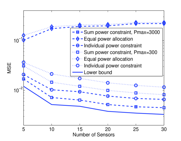
Refer to caption
Figure 1: MSE vs. number of sensors for Pmax=300subscript𝑃300P_{\max}=300 or 300030003000.
Refer to caption
Figure 2: Required sum transmit power vs. number of sensors for various MSE constraints.
Refer to caption
Figure 3: Maximum individual transmit power vs. number of sensors for various MSE constraints.
Refer to caption
Figure 4: Exact and approximate sum transmit power vs. number of sensors.
Refer to caption
Figure 5: Stem plot for the channel gain, measurement noise variance and the individual transmit power allocated to the sensor nodes. The x-axis denotes the sensor node ID and the sensor nodes are indexed according to their channel gain, in ascending order. For the high SNR case the total transmit power is set to PT=1000subscript𝑃𝑇1000P_{T}=1000 and for the low SNR case the total transmit power is PT=5subscript𝑃𝑇5P_{T}=5.
Refer to caption
Figure 6: MSE outage probability for equal power allocation vs. sum transmit power for N=10𝑁10N=10 sensors.