Transmuted Generalized Inverse Weibull Distribution

Abstract.

A generalization of the generalized inverse Weibull distribution so-called transmuted generalized inverse Weibull distribution is proposed and studied. We will use the quadratic rank transmutation map (QRTM) in order to generate a flexible family of probability distributions taking generalized inverse Weibull distribution as the base value distribution by introducing a new parameter that would offer more distributional flexibility. Various structural properties including explicit expressions for the moments, quantiles, and moment generating function of the new distribution are derived.We proposed the method of maximum likelihood for estimating the model parameters and obtain the observed information matrix. A real data set are used to compare the flexibility of the transmuted version versus the generalized inverse Weibull distribution.

Keywords: Generalized Inverse Weibull Distribution, Order Statistics,Transmutation map, Maximum Likelihood Estimation, Reliability Function.

1. Introduction

The inverse Weibull distribution is another life time probability distribution which can be used in the reliability engineering discipline. The inverse Weibull distribution can be used to model a variety of failure characteristics such as infant mortality, useful life and wear- out periods. It can also be used to determine the cost effectiveness , maintenance periods of reliability centered maintenance activities and applications in medicine, reliability and ecology. Keller (1985) obtained the inverse Weibull model by investigating failures of mechanical components subject to degradation. Drapella (1993), Mudholkar and Kollia (1994) and Gusmão et al. (2011) introduced the generalized inverse Weibull distribution, among others. The cumulative distribution function (cdf) of the generalized inverse Weibull (GIW) distribution can be defined by

(1) $$G(x,\alpha,\gamma,\theta)=e^{-\gamma(\alpha x)^{-\beta}},\alpha>0,\gamma>0,\beta>0\text{ and }x\geq 0.$$

where $\alpha$ is scale parameter and $\beta,\gamma$ are shape parameters respectively. The corresponding probability density function (pdf) is given by

(2) $$g(x,\alpha,\gamma,\theta)=\alpha\beta\gamma(\alpha x)^{-\beta-1}e^{-\gamma(\alpha x)^{-\beta}}.$$

In this article we present a new generalization of generalized inverse Weibull distribution called the transmuted generalized inverse Weibull distribution. We will derive the subject distribution using the quadratic rank transmutation map studied by Shaw et al. (2007). A random variable $X$ is said to have transmuted distribution if its cumulative distribution function(cdf) is given by

(3) $$F(x)=(1+\lambda)G(x)-\lambda G(x)^{2},\left|\lambda\right|\leq 1,$$

where $G(x)$ is the cdf of the base distribution, which on differentiation yields,

(4) $$f(x)=g(x)\left[(1+\lambda)-2\lambda G(x)\right]$$

where $f(x)$ and $g(x)$ are the corresponding pdfs associated with cdf $F(x)$ and $G(x)$ respectively. An extensive information about the quadratic rank transmutation map is given in Shaw et al. (2007). Observe that at $\lambda=0$ we have the distribution of the base random variable.

Many authors dealing with the generalization of some well- known distributions. Aryal and Tsokos (2009) defined the transmuted generalized extreme value distribution and they studied some basic mathematical characteristics of transmuted Gumbel probability distribution and it has been observed that the transmuted Gumbel can be used to model climate data. Also Aryal and Tsokos (2011) presented a new generalization of Weibull distribution called the transmuted Weibull distribution . Recently, Aryal (2013) proposed and studied the various structural properties of the transmuted Log- Logistic distribution. and Khan and King (2013) introduced the transmuted modified Weibull distribution which extended recent development on transmuted Weibull distribution by Aryal et al. (2011), and they studied the mathematical properties and maximum likelihood estimation of the unknown parameters. In the present study we will provide mathematical formulation of the transmuted generalized inverted exponential distribution and some of its properties. We will also provide possible area of applications.

The rest of the paper is organized as follows. In Section 3 we demonstrate transmuted probability distribution. In Section 4 , we find the reliability functions of the subject model. The statistical properties include quantile functions, moments and moment generating functions are derived in Section 5.The minimum, maximum and median order statistics models are discussed in Section 6. Least Squares and Weighted Least Squares Estimators are discused in section 7.Section 8 we demonstrate the maximum likelihood estimates and the asymptotic confidence intervals of the unknown parameters. In section 9, the TGIW distribution is applied to a real data set. Finally, in Section 10, we provide some conclusion.

2. Transmutation Map

In this section we demonstrate transmuted probability distribution. Let $F_{1}$ and $F_{2}$ be the cumulative distribution functions, of two distributions with a common sample space. The general rank transmutation as given in (2007) is defined as

$$G_{R12}(u)=F_{2}(F_{1}^{-1}(u))\text{ \ and }G_{R21}(u)=F_{1}(F_{2}^{-1}(u)).$$

Note that the inverse cumulative distribution function also known as quantile function is defined as

$$F^{-1}(y)=\text{ inf}_{x\in R}\left\{F(x)\geq y\right\}\text{ for }y\in\left[0,1\right].$$

The functions $G_{R12}(u)$ and $G_{R21}(u)$ both map the unit interval $I=$ $\left[0,1\right]$ into itself, and under suitable assumptions are mutual inverses and they satisfy $G_{Rij}(0)=0$ and $G_{Rij}(0)=1.$ A quadratic Rank Transmutation Map (QRTM) is defined as

(5) $$G_{R12}(u)=u+\lambda u(1-u),\left|\lambda\right|\leq 1,$$

from which it follows that the cdf’s satisfy the relationship

(6) $$F_{2}(x)=(1+\lambda)F_{1}(x)-\lambda F_{1}(x)^{2}$$

which on differentiation yields,

(7) $$f_{2}(x)=f_{1}(x)\left[(1+\lambda)-2\lambda F_{1}(x)\right]$$

where $f_{1}(x)$ and $f_{2}(x)$ are the corresponding pdfs associated with cdf $F_{1}(x)$ and $F_{2}(x)$ respectively. An extensive information about the quadratic rank transmutation map is given in Shaw et al. (2007). Observe that at $\lambda=0$ we have the distribution of the base random variable. The function $f_{2}(x)$ in given (7) satisfies the property of probability density function.

3. Transmuted Generalized Inverse Weibull Distribution

In this section we studied the transmuted generalized inverse weibull (TGIW) Distribution and the sub-models of this distribution. Now using (1) and (2) we have the cdf of transmuted generalized inverted exponential distribution

(8) $$F_{TGIW}(x)=e^{-\gamma(\alpha x)^{-\beta}}\left[1+\lambda-\lambda e^{-\gamma(\alpha x)^{-\beta}}\right]$$

where $\alpha$ is scale parameter and $\beta,\gamma$ are shape parameters representing the different patterns of the transmuted generalized inverse weibull distribution and $\lambda$ is the transmuted parameter.The corresponding probability density function (pdf) of the transmuted generalized inverse Weibull distribution is given by

(9) $$f_{TGIW}(x)=\alpha\beta\gamma(\alpha x)^{-\beta-1}e^{-\gamma(\alpha x)^{-\beta}}\left[1+\lambda-2\lambda e^{-\gamma(\alpha x)^{-\beta}}\right].$$

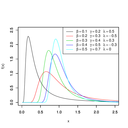
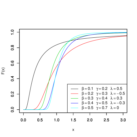
Figure 1 and 2 illustrates some of the possible shapes of the pdf and cdf of TGIW distribution for selected values of the parameters $\beta,\gamma$ and $\lambda,$ by keeping $alpha=1$, respectively.

Figure 1. The pdf’s of various TGIW distributions.

Figure 2. The cdf of various TGIW distributions.

The transmuted generalized inverse Weibull distribution is very flexible model that approaches to different distributions when its parameters are changed. The flexibility of the transmuted generalized inverse Weibull distribution is explained in the following . If $X$ is a random variable with pdf (9), then we have the following cases.

1. If $\gamma=1,$we get the transmuted inverse Weibull.

2. If $\lambda=0$ and $\gamma=1,$we get the inverse Weibull.

3. If $\beta=1$ , $\gamma=1$we get the transmuted inverse exponential distribution.

4. If $\beta=1$ , $\gamma=1$ and $\lambda=0$ we get the inverse exponential distribution.

5. If $\beta=2$ , $\gamma=1$ we get transmuted inverse Rayleigh distribution.

6. If $\beta=2$ , $\gamma=1$ and $\lambda=0$ we get the inverse Rayleigh distribution.

7. If $\alpha=1$ we get the transmuted Frechet distribution.

8. If $\alpha=1$ and and $\lambda=0$ we get Frechet distribution.

4. Reliability Analysis

The reliability function $R(x)$, which is the probability of an item not failing prior to some time $t$, is defined by $R(x)=1-F(x)$. The reliability function of a transmuted generalized inverse Weibull distribution $R_{TGIW}(x)$, it can be a useful characterization of life time data analysis.

$$R_{TGIW}(x) =1-F_{TGIW}(x)$$

(10) $$=1-e^{-\gamma(\alpha x)^{-\beta}}\left[1+\lambda-\lambda e^{-\gamma(\alpha x)^{-\beta}}\right].$$

It is important to note that $R_{TGIW}(x)+F_{TGIW}(x)=1$ . The other characteristic of interest of a random variable is the hazard rate function defined by $h_{TGIW}(x)=\frac{f_{TGIW}(x)}{1-F_{TGIW}(x)}$ which is an important quantity characterizing life phenomenon. It can be loosely interpreted as the conditional probability of failure, given it has survived to the time $t$. The hazard rate function for a transmuted generalized inverse Weibull distribution is defined by

$$h_{TGIW}(x) =\frac{f_{TGIW}(x)}{1-F_{TGIW}(x)}$$

(11) $$=\frac{\alpha\beta\gamma(\alpha x)^{-\beta-1}e^{-\gamma(\alpha x)^{-\beta}}\left[1+\lambda-2\lambda e^{-\gamma(\alpha x)^{-\beta}}\right]}{1-e^{-\gamma(\alpha x)^{-\beta}}\left[1+\lambda-\lambda e^{-\gamma(\alpha x)^{-\beta}}\right].}$$

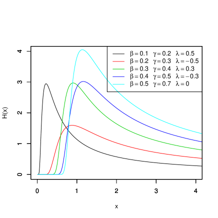
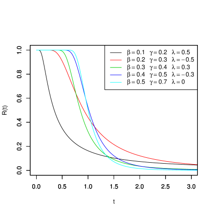
Figure 3 and 4 illustrates some of the possible shapes of the hazard rate function and survival function of TGIW distribution for selected values of the parameters $\beta,\gamma$ and $\lambda,$ by keeping $alpha=1$, respectively.

Figure 3. The hazard function of various TGIW distributions

Figure 4. The survival function of various TGIW distributions

It is important to note that the units for $h_{TGIW}(x)$ is the probability of failure per unit of time, distance or cycles. These failure rates are defined with different choices of parameters.The cumulative hazard function of the transmuted generalized inverse Weibull distribution is denoted by

(12) $$H_{TGIW}(x)=-\ln\left|e^{-\gamma(\alpha x)^{-\beta}}\left[1+\lambda-\lambda e^{-\gamma(\alpha x)^{-\beta}}\right]\right|$$

It is important to note that the units for $H_{TGIW}(x)$ is the cumulative probability of failure per unit of time, distance or cycles.

5. Statistical Properties

In this section we discuss the statistical properties of the transmuted generalized inverse Weibull distribution. Specifically quantile and random number generation function, moments and moment generating function.

5.1. Quantile and Median

The quantile $x_{q}$ of the $T_{GIW}$ $(\alpha,\beta,\gamma,\lambda,x)$ is real solution of the following equation

(13) $$x_{q}=\left\{\frac{-1}{\gamma}\ln\left(\frac{(\lambda+1)+\sqrt{(\lambda+1)^{2}-4\lambda q}}{2\lambda}\right)\right\}^{\frac{-1}{\beta}}$$

The above equation has no closed form solution in $x_{q}$, so we have to use a numerical technique such as a Newton- Raphson method to get the quantile. If we put $q=0.5$ in equation (13) one gets the median of $T_{GIW}(\alpha,\beta,\gamma,\lambda,x)$

5.2. Random Number Generation

The random number generation as $x$ of the $T_{GIW}(\alpha,\beta,\gamma,\lambda,x)$ is defined by the following relation

(14) $$x_{q}=\left\{\frac{-1}{\gamma}\ln\left(\frac{(\lambda+1)+\sqrt{(\lambda+1)^{2}-4\lambda\phi}}{2\lambda}\right)\right\}^{\frac{-1}{\beta}}\text{\ where }\phi\sim U(0,1).$$

5.3. Moments

The following theorem gives the $r_{th}$ moment $(\mu_{r}^{{}^{\prime}})$ of the $T_{GIW}$ $(\alpha,\beta,\gamma,\lambda,x).$

Theorem (4.1). If $X$ has the $T_{GIW}(\alpha,\beta,\gamma,\lambda,x)$ with $\left|\lambda\right|\leq 1$, then the $r_{th}$ non central moments are given by

(15) $$\mu_{r}^{{}^{\prime}}(x)=E(X^{r})=\frac{\gamma^{\frac{r}{\beta}}\Gamma(1-\frac{r}{\beta})}{\alpha^{r}}\left[1+\lambda-\lambda(2)^{\frac{r}{\beta}}\right].$$

Proof:
Starting with

$$\mu_{r}^{{}^{\prime}}(x) =\int\nolimits_{0}^{\infty}x^{r}f_{TGIW}(\alpha,\beta,\gamma,\lambda,x)dx$$

$$=\int\limits_{0}^{\infty}x^{r}\alpha\beta\gamma(\alpha x)^{-\beta-1}e^{-\gamma(\alpha x)^{-\beta}}\left[1+\lambda-2\lambda e^{-\gamma(\alpha x)^{-\beta}}\right]$$

$$=\left\{\frac{\alpha\beta\gamma}{\alpha^{r}}\left(1+\lambda\right)\int\nolimits_{0}^{\infty}(\alpha x)^{r-\beta-1}e^{-\gamma(\alpha x)^{-\beta}}dx\right.$$

(16) $$-\left.\frac{2\lambda\alpha\beta\gamma}{\alpha^{r}}\int\limits_{0}^{\infty}(\alpha x)^{r-\beta-1}e^{-2\gamma(\alpha x)^{-\beta}}dx\right\}$$

let $\gamma(\alpha x)^{-\beta}=t$ then $x=\frac{1}{\alpha}\gamma^{\frac{1}{\beta}}t^{\frac{-1}{\beta}},$ therefore

$$\mu_{r}^{{}^{\prime}}(x) =\frac{\left(1+\lambda\right)}{\alpha^{r}}\gamma^{\frac{r}{\beta}}\Gamma(1-\frac{r}{\beta})-\frac{\lambda}{\alpha^{r}}(2\gamma)^{\frac{r}{\beta}}\Gamma(1-\frac{r}{\beta})$$

(17) $$=\frac{\gamma^{\frac{r}{\beta}}\Gamma(1-\frac{r}{\beta})}{\alpha^{r}}\left[1+\lambda-\lambda(2)^{\frac{r}{\beta}}\right].$$

Which completes the proof.

Based on Theorem (4.1) the coefficient of variation, coefficient of skewness and coefficient of kurtosis of $T_{GIW}$ $(\alpha,\beta,\gamma,\lambda,x)$ distribution can be obtained according to the following relation

$$CV_{TMIW} =\sqrt{\frac{\mu_{2}}{\mu_{1}}-1},$$

$$CS_{TMIW} =\frac{\mu_{3}-3\mu_{2}\mu_{1}+2\mu_{1}^{3}}{(\mu_{2}-\mu_{1})^{\frac{3}{2}}}$$

$$\text{and}CK_{TMIW} =\frac{\mu_{4}-4\mu_{3}\mu_{1}+6\mu_{2}\mu_{1}^{2}}{(\mu_{2}-\mu_{1}^{2})^{2}}.$$

5.4. Moment Generating Function

In this subsection we derived the moment generating function (mgf) of transmuted generalized inverse Weibull distribution.
Theorem (4.2): If $X$ has the$T_{GIW}$ $(\alpha,\beta,\gamma,\lambda,x)$ with $\left|\lambda\right|\leq 1$, then the the moment generating function (mgf) of $X$  is given as follows

(18) $$M_{X}(t)=\sum\limits_{r=0}^{\infty}\frac{t^{r}\gamma^{\frac{r}{\beta}}\Gamma(1-\frac{r}{\beta})}{r!\alpha^{r}}\left[1+\lambda-\lambda(2)^{\frac{r}{\beta}}\right].$$

Proof:

$$M_{X}(t) =\int\nolimits_{0}^{\infty}e^{tx}f_{T_{GIW}}(\alpha,\beta,\gamma,\lambda,x)dx$$

$$=\sum\nolimits_{r=0}^{\infty}\frac{t^{r}}{r!}\text{ }x^{r}f_{T_{GIW}}(\alpha,\beta,\gamma,\lambda,x)dx$$

(19) $$=\sum\nolimits_{r=0}^{\infty}\frac{t^{r}}{r!}\mu_{r}^{{}^{\prime}}(x)$$

using equations (15) into relation (5.4) we get the following

$$M_{X}(t)=\sum\limits_{r=0}^{\infty}\frac{t^{r}\gamma^{\frac{r}{\beta}}\Gamma(1-\frac{r}{\beta})}{r!\alpha^{r}}\left[1+\lambda-\lambda(2)^{\frac{r}{\beta}}\right].$$

Which completes the proof.

6. Order Statistics

In fact, the order statistics have many applications in reliability and life testing. The order statistics arise in the study of reliability of a system. Let $X_{1},X_{2},...,X_{n}$ be a simple random sample from $T_{GIW}$ $(\alpha,\beta,\gamma,\lambda,x)$ with cumulative distribution function and probability density function as in (8) and (9), respectively. Let $X_{(1:n)}\leq X_{(2:n)}\leq\ldots\leq X_{(n:n)}$ denote the order statistics obtained from this sample. In reliability literature, $X_{(i:n)}$ denote the lifetime of an $(n-i+1)-$ out$-$ of$-$ $n$ system which consists of $n$ independent and identically components. Then the pdf of $X_{(i:n)}$ $,1\leq i\leq n$ is given by

(20) $$f_{i::n}(x)=\frac{1}{\beta(i,n-i+1)}\left[F(x,\Phi)\right]^{i-1}\left[1-F(x,\Phi)\right]^{n-i}f(x,\Phi)$$

where $\Phi=((\alpha,\beta,\gamma,\lambda)$. Also, the joint pdf of $X_{(i:n)},X_{(j:n)}$ and $1\leq i\leq j\leq n$ is

(21) $$f_{i:j:n}(x_{i},x_{j})=C\text{ }\left[F(x_{i})\right]^{i-1}\left[F(x_{j})-F(x_{i})\right]^{j-i-1}\left[1-F(x_{j})\right]^{n-j}f(x_{i})f(x_{j})$$

where

$$C=\frac{n!}{(i-1)!(j-i-1)!(n-j)!}$$

We defined the first order statistics $X_{(1)}=Min(X_{1},X_{2},\ldots,X_{n}),$ the last order statistics as $X_{(n)}=Max(X_{1},X_{2},\ldots,X_{n})$ and median order $X_{m+1}$ .

6.1. Distribution of Minimum , Maximum and Median

Let $X_{1},X_{2},\ldots,X_{n}$ be independently identically distributed order random variables from the transmuted generalized inverse weibull distribution having first , last and median order probability density function are given by the following

$$f_{1:n}(x) =n\left[1-F(x,\Phi)\right]^{n-1}f(x,\Phi)$$

$$=n\left\{1-e^{-\gamma(\alpha x_{(1)})^{-\beta}}\left[1+\lambda-\lambda e^{-\gamma(\alpha x_{(1)})^{-\beta}}\right]\right\}^{n-1}$$

(22) $$\times\alpha\beta\gamma(\alpha x_{(1)})^{-\beta-1}e^{-\gamma(\alpha x_{(1)})^{-\beta}}\left[1+\lambda-2\lambda e^{-\gamma(\alpha x_{(1)})^{-\beta}}\right]$$

$$f_{n:n}(x) =n\left[F(x_{(n)},\Phi)\right]^{n-1}f(x_{(n)}),\Phi)$$

$$=n\left\{e^{-\gamma(\alpha x_{(n)})^{-\beta}}\left[1+\lambda-\lambda e^{-\gamma(\alpha x_{(n)})^{-\beta}}\right]\right\}^{n-1}$$

(23) $$\times\alpha\beta\gamma(\alpha x_{(n)})^{-\beta-1}e^{-\gamma(\alpha x_{(n)})^{-\beta}}\left[1+\lambda-2\lambda e^{-\gamma(\alpha x_{(n)})^{-\beta}}\right]$$

and

$$f_{m+1:n}(\widetilde{x}) =\frac{(2m+1)!}{m!m!}(F(\widetilde{x}))^{m}(1-F(\widetilde{x}))^{m}f(\widetilde{x})$$

$$=\frac{(2m+1)!}{m!m!}\left\{e^{-\gamma(\alpha x_{(m+1)})^{-\beta}}\left[1+\lambda-\lambda e^{-\gamma(\alpha x_{(m+1)})^{-\beta}}\right]\right\}^{m}$$

$$\times\left\{1-e^{-\gamma(\alpha x_{(m+1)})^{-\beta}}\left[1+\lambda-\lambda e^{-\gamma(\alpha x_{(m+1)})^{-\beta}}\right]\right\}^{m}$$

(24) $$\times\alpha\beta\gamma(\alpha x_{(m+1)})^{-\beta-1}e^{-\gamma(\alpha x_{(m+1)})^{-\beta}}\left[1+\lambda-2\lambda e^{-\gamma(\alpha x_{(m+1)})^{-\beta}}\right]$$

6.2. Joint Distribution of the i_th and j_th order Statistics

The joint distribution of the the $i_{th}$ and $j_{th}$ order statistics from transmuted generalized inverse Weibull is

$$f_{i:j:n}(x_{i},x_{j}) =C\text{ }\left[F(x_{i})\right]^{i-1}\left[F(x_{j})-F(x_{i})\right]^{j-i-1}\left[1-F(x_{j})\right]^{n-j}f(x_{i})f(x_{j})$$

$$=C\left\{h_{(i)}\left[1+\lambda-\lambda h_{(i)}\right]\right\}^{i-1}$$

$$\times\left\{h_{(j)}\left[1+\lambda-\lambda h_{(j)}\right]-h_{(i)}\left[1+\lambda-\lambda h_{(i)}\right]\right\}^{j-i-1}$$

$$\times\left\{1-h_{(j)}\left[1+\lambda-\lambda h_{(j)}\right]\right\}^{n-j}$$

$$\alpha\beta\gamma(\alpha x_{(1)})^{-\beta-1}e^{-\gamma(\alpha x_{(1)})^{-\beta}}\left[1+\lambda-2\lambda e^{-\gamma(\alpha x_{(1)})^{-\beta}}\right]$$

$$\times\alpha\beta\gamma(\alpha x_{(i)})h_{(i)}\left[1+\lambda-2\lambda h_{(i)}\right]$$

(25) $$\times\alpha\beta\gamma(\alpha x_{(j)})h_{(j)}\left[1+\lambda-2\lambda h_{(j)}\right]$$

where

$$h_{(i)}=e^{-\gamma(\alpha x_{(i)})^{-\beta}}$$

special case if $i=1$ and $j=n$ we get the joint distribution of the minimum and maximum of order statistics

$$f_{1::n:n}(x_{i},x_{j}) =n(n-1)\text{ }\left[F(x_{(n)})-F(x_{(1)})\right]^{n-2}f(x_{(1)})f(x_{(n)})$$

$$=n(n-1)\left\{h_{(n)}\left[1+\lambda-\lambda h_{(n)}\right]-h_{(1)}\left[1+\lambda-\lambda h_{(1)}\right]\right\}^{n-2}$$

$$\times\alpha\beta\gamma(\alpha x_{(1)})h_{(1)}\left[1+\lambda-2\lambda h_{(i1}\right]$$

(26) $$\times\alpha\beta\gamma(\alpha x_{(n)})h_{(n)}\left[1+\lambda-2\lambda h_{(n)}\right].$$

7. Least Squares and Weighted Least Squares Estimators

In this section we provide the regression based method estimators of the unknown parameters of the transmuted generalized inverse Weibull distribution, which was originally suggested by Swain, Venkatraman and Wilson (1988) to estimate the parameters of beta distributions. It can be used some other cases also. Suppose $Y_{1},...,Y_{n}$ is a random sample of size $n$ from a distribution function $G(.)$ and suppose $Y_{(i)};i=1,2,...,n$ denotes the ordered sample. The proposed method uses the distribution of $G(Y_{(i)})$. For a sample of size $n$, we have

$$E\left(G(Y_{(j)})\right) =\frac{j}{n+1},V\left(G(Y_{(j)})\right)=\frac{j(n-j+1)}{(n+1)^{2}(n+2)}$$

$$\text{and }Cov\left(G(Y_{(j)}),G(Y_{(k)})\right)=\frac{j(n-k+1)}{(n+1)^{2}(n+2)};\text{for\ }j<k\text{,}$$

see Johnson, Kotz and Balakrishnan (1995). Using the expectations and the variances, two variants of the least squares methods can be used.

Method 1 (Least Squares Estimators) . Obtain the estimators by minimizing

(27) $$\sum\nolimits_{j=1}^{n}\left(G(Y_{(j)}-\frac{j}{n+1}\right)^{2},$$

with respect to the unknown parameters. Therefore in case of $TGIW$ distribution the least squares estimators of $\alpha,\beta$ and $\lambda$ , say $\widehat{\alpha}_{LSE},\widehat{\beta}_{LSE}$ and $\widehat{\lambda}_{LSE}$ respectively, can be obtained by minimizing

$$\sum\limits_{j=1}^{n}\left[e^{-\gamma(\alpha x_{(i)})^{-\beta}}\left[1+\lambda-\lambda e^{-\gamma(\alpha x_{(i)})^{-\beta}}\right]-\frac{j}{n+1}\right]^{2}$$

with respect to $\alpha,$ $\beta$ and $\lambda$ .

Method 2 (Weighted Least Squares Estimators). The weighted least squares estimators can be obtained by minimizing

(28) $$\sum\limits_{j=1}^{n}w_{j}\left(G(Y_{(j)}-\frac{j}{n+1}\right)^{2},$$

with respect to the unknown parameters, where

$$w_{j}=\frac{1}{V\left(G(Y_{(j)})\right)}=\frac{(n+1)^{2}(n+2)}{j(n-j+1)}.$$

Therefore, in case of $TGIW$ distribution the weighted least squares estimators of $\alpha,\beta$ and $\lambda$ , say $\widehat{\alpha}_{WLSE},\widehat{\beta}_{WLSE}$ and $\widehat{\lambda}_{WLSE}$ respectively, can be obtained by minimizing

$$\sum\limits_{j=1}^{n}w_{j}\left[e^{-\gamma(\alpha x_{(i)})^{-\beta}}\left[1+\lambda-\lambda e^{-\gamma(\alpha x_{(i)})^{-\beta}}\right]-\frac{j}{n+1}\right]^{2}$$

with respect to the unknown parameters only.

8. Maximum Likelihood Estimators

In this section we discuss the maximum likelihood estimators (MLE’s) and inference for the $T_{GIW}$ $(\alpha,\beta,\gamma,\lambda,x)$ distribution. Let $x_{1},...,x_{n}$ be a random sample of size $n$ from $T_{GIW}$ $(\alpha,\beta,\gamma,\lambda,x)$ then the likelihood function can be written as

(29) $$L(\alpha,\beta,\gamma,\lambda,x_{{}_{(i)}})=\prod\limits_{i=1}^{n}\alpha\beta\gamma(\alpha x_{(i)})^{-\beta-1}e^{-\gamma(\alpha x_{(i)})^{-\beta}}\left[1+\lambda-2\lambda e^{-\gamma(\alpha x_{(i)})^{-\beta}}\right]dx$$

By accumulation taking logarithm of equation (6.1) , and the log- likelihood function can be written as

$$\log L =n\ln\alpha+n\ln\beta+n\ln\gamma-(\beta+1)\sum\nolimits_{i=1}^{n}\ln(\alpha x_{(i)})$$

(30) $$-\gamma\sum\nolimits_{i=1}^{n}(\alpha x_{(i)})^{-\beta}+\sum\nolimits_{i=1}^{n}\ln\left[1+\lambda-2\lambda e^{-\gamma(\alpha x_{(i)})^{-\beta}}\right]$$

Differentiating equation (8) with respect to $\alpha,\beta,\gamma,$ and $\lambda$ then equating it to zero. The normal equations become

$$\frac{\partial\log L}{\partial\alpha} =\frac{n}{\alpha}-(\beta+1)\sum\limits_{i=1}^{n}(\frac{1}{\alpha})+\gamma\beta\sum\limits_{i=1}^{n}x_{(i)}(\alpha x_{(i)})^{-\beta-1}$$

(31) $$-\sum\limits_{i=1}^{n}\frac{2\lambda\alpha x_{(i)}(\alpha x_{(i)})^{-\beta-1}e^{-\gamma(\alpha x_{(i)})^{-\beta}}}{\left[1+\lambda-2\lambda e^{-\gamma(\alpha x_{(i)})^{-\beta}}\right]}=0,$$

$$\frac{\partial\log L}{\partial\beta} =\frac{n}{\beta}-\sum\limits_{i=1}^{n}\ln(\alpha x_{(i)})+\gamma\sum\limits_{i=1}^{n}(\alpha x_{(i)})^{-\beta}\ln(\alpha x_{(i)})$$

(32) $$+\sum\limits_{i=1}^{n}\frac{-2\lambda\gamma e^{-\gamma(\alpha x_{(i)})^{-\beta}}(\alpha x_{(i)})^{-\beta}\ln(\alpha x_{(i)})}{\left[1+\lambda-2\lambda e^{-\gamma(\alpha x_{(i)})^{-\beta}}\right]}=0,$$

(33) $$\frac{\partial\log L}{\partial\gamma}=\frac{n}{\gamma}-\sum\limits_{i=1}^{n}(\alpha x_{(i)})^{-\beta}+\sum\nolimits_{i=1}^{n}\frac{2\lambda e^{-\gamma(\alpha x_{(i)})^{-\beta}}(\alpha x_{(i)})^{-\beta}}{\left[1+\lambda-2\lambda e^{-\gamma(\alpha x_{(i)})^{-\beta}}\right]}=0,$$

and

(34) $$\frac{\partial\log L}{\partial\lambda}=\sum\limits_{i=1}^{n}\frac{1-2e^{-\gamma(\alpha x_{(i)})^{-\beta}}}{\left[1+\lambda-2\lambda e^{-\gamma(\alpha x_{(i)})^{-\beta}}\right]}.$$

We can find the estimates of the unknown parameters by maximum likelihood method by setting these above nonlinear system of equations (8) - (34) to zero and solve them simultaneously. These solutions will yield the ML estimators for $\widehat{\alpha}$,$\widehat{\theta}$ , and $\widehat{\lambda}.$ For the three parameters transmuted generalized inverted Weibull distribution $T_{GIW}$ $(\alpha,\beta,\gamma\lambda,x)$ pdf, all the second order derivatives exist. Thus we have the inverse dispersion matrix is given by

(35) $$\left(\begin{array}[]{c}\widehat{\alpha}\\ \widehat{\beta}\\ \widehat{\gamma}\\ \widehat{\lambda}\end{array}\right)\sim N\left[\left(\begin{array}[]{c}\alpha\\ \beta\\ \gamma\\ \lambda\end{array}\right),\left(\begin{array}[]{cccc}\widehat{V_{\alpha\alpha}}&\widehat{V_{\alpha\beta}}&\widehat{V_{\alpha\gamma}}&\widehat{V_{\alpha\lambda}}\\ \widehat{V_{\beta\alpha}}&\widehat{V_{\beta\beta}}&\widehat{V_{\beta\gamma}}&\widehat{V_{\beta\lambda}}\\ \widehat{V_{\gamma\alpha}}&\widehat{V_{\gamma\beta}}&\widehat{V_{\gamma\gamma}}&\widehat{V_{\gamma\lambda}}\\ \widehat{V_{\lambda\alpha}}&\widehat{V_{\lambda\beta}}&\widehat{V_{\lambda\gamma}}&\widehat{V_{\lambda\lambda}}\end{array}\right)\right].$$

$$V^{-1}=-E\left[\begin{tabular}[]{cccc}$V_{\alpha\alpha}$&$V_{\alpha\beta}$&$V_{\alpha\gamma}$&$V_{\alpha\lambda}$\\ &$V_{\beta\beta}$&$V_{\beta\gamma}$&$V_{\beta\lambda}$\\ &&$V_{\gamma\gamma}$&$V_{\gamma\lambda}$\\ &&&$V_{\lambda\lambda}$\\ \end{tabular}\right]$$

where

$$V_{\alpha\alpha} =\frac{\partial^{2}L}{\partial\alpha^{2}},V_{\beta\beta}=\frac{\partial^{2}L}{\partial\beta^{2}},V_{\lambda\lambda}=\frac{\partial^{2}L}{\partial\lambda^{2}},V_{\alpha\beta}=\frac{\partial^{2}L}{\partial\alpha\partial\beta}$$

$$V_{\lambda\alpha} =\frac{\partial^{2}L}{\partial\alpha\partial\lambda},$$

By solving this inverse dispersion matrix these solutions will yield asymptotic variance and covariances of these ML estimators for $\widehat{\alpha}$,$\widehat{\beta}$ , $\widehat{\gamma}$ and $\widehat{\lambda}.$ Using (35), we approximate $100(1-\delta)\%$ confidence intervals for $\alpha,\beta,\gamma$ and $\lambda$ are determined respectively as

$$\widehat{\alpha}\pm z_{\frac{\delta}{2}}\sqrt{\widehat{V_{\alpha\alpha}}},\text{ }\widehat{\beta}\pm z_{\frac{\delta}{2}}\sqrt{\widehat{V_{\beta\beta}}}\text{\ , }\widehat{\gamma}\pm z_{\frac{\delta}{2}}\sqrt{\widehat{V_{\gamma\gamma}}}\text{and }\widehat{\lambda}\pm z_{\frac{\delta}{2}}\sqrt{\widehat{V_{\lambda\lambda}}}$$

where $z_{\delta}$ is the upper $100\delta_{the}$ percentile of the standard normal distribution.

We can compute the maximized unrestricted and restricted log-likelihood functions to construct the likelihood ratio (LR) test statistic for testing on some transmuted GIW sub-models. For example, we can use the LR test statistic to check whether the TGIW distribution for a given data set is statistically superior to the GIW distribution. In any case, hypothesis tests of the type $H_{0}:\theta=\theta_{0}$ versus $H_{0}:\theta\neq\theta_{0}$ can be performed using a LR test. In this case, the LR test statistic for testing $H_{0}$ versus $H_{1}$ is $\omega=2(\ell(\hat{\theta};x)-\ell(\hat{\theta}_{0};x))$, where $\hat{\theta}$ and $\hat{\theta}_{0}$ are the MLEs under $H_{1}$ and $H_{0}$, respectively. The statistic $\omega$ is asymptotically (as $n\to\infty$) distributed as $\chi^{2}_{k}$, where $k$ is the length of the parameter vector $\theta$ of interest. The LR test rejects $H_{0}$ if $\omega>\chi^{2}_{k;\gamma}$, where $\chi^{2}_{k;\gamma}$ denotes the upper $100\gamma\%$ quantile of the $\chi^{2}_{k}$ distribution.

9. Aplication

In this section, we use a real data set to show that the TGIW distribution can be a better model than one based on the GIW distribution. The data set given in Table 1 taken from [14] page 180 represents 50 items put into use at $t=0$ and failure times are in weeks.

Table 1. 50 items put into use at $t=0$ and failure times are in weeks.

0.013	0.065	0.111	0.111	0.163	0.309	0.426	0.535	0.684	0.747
0.997	1.284	1.304	1.647	1.829	2.336	2.838	3.269	3.977	3.981
4.520	4.789	4.849	5.202	5.291	5.349	5.911	6.018	6.427	6.456
6.572	7.023	7.087	7.291	7.787	8.596	9.388	10.261	10.713	11.658
13.006	13.388	13.842	17.152	17.283	19.418	23.471	24.777	32.795	48.105

Table 2. Estimated parameters of the GIW and TGIW distribution for 50 items put into use at $t=0$ and failure times are in weeks.

Model	Parameter Estimate	$-\ell(\cdot;x)$
GIW	$\hat{\alpha}=0.8537419$,$\hat{\beta}=0.4790610$	168.638
	$\hat{\gamma}=1.043654$
TGIW	$\hat{\alpha}=2.382715$, $\hat{\beta}=0.5297876$	166.387
	$\hat{\gamma}=1.1428575$, $\hat{\lambda}=-0.7472070$

Table 3. Criteria for comparison.

Model	K-S	$-2\ell$	AIC	AICC
GIW	0.1992	337.276	343.276	343.797
TGIW	0.1917	332.774	340.774	341.662

The LR test statistic to test the hypotheses $H_{0}:\lambda=0$ versus $H_{1}:\lambda\not=0$ is $\omega=4.502>3.841=\chi^{2}_{1;0.05}$, so we reject the null hypothesis. In order to compare the two distribution models, we consider criteria like K-S, $-2\ell$, AIC (Akaike information criterion)and AICC (corrected Akaike information criterion) for the data set. The better distribution corresponds to smaller $-2\ell$, AIC and AICC values:‘

$$\mbox{AIC}=2k-2\ell\,,\quad\textrm{and}\mbox{AICC}=\mbox{AIC}+\frac{2k(k+1)}{n-k-1}\,,$$

where $k$ is the number of parameters in the statistical model, $n$ the sample size and $\ell$ is the maximized value of the log-likelihood function under the considered model. Table 2 shows the MLEs under both distributions, table 3 shows the values of K-S, $-2\ell$, AIC and AICC values. The values in table 3 indicate that the TGIW distribution leads to a better fit than the GIW distribution .

10. Conclusion

Here we propose a new model, the so-called the transmuted generalized inverse Weibull distribution which extends the generalized inverse Weibull distribution in the analysis of data with real support. An obvious reason for generalizing a standard distribution is because the generalized form provides larger flexibility in modeling real data. We derive expansions for moments and for the moment generating function. The estimation of parameters is approached by the method of maximum likelihood, also the information matrix is derived. An application of TGIW distribution to real data show that the new distribution can be used quite effectively to provide better fits than GIW distribution.

References

• [1] Aryal, G. R., and Tsokos, C. P. (2009). On the transmuted extreme value distribution with application. Nonlinear Analysis: Theory, Methods and Applications, 71(12), e1401-e1407.
• [2] Aryal, G. R., and Tsokos, C. P. (2011). Transmuted Weibull Distribution: A Generalization of theWeibull Probability Distribution. European Journal of Pure and Applied Mathematics, 4(2), 89-102.
• [3] Barlow R. E., and Proschan F. (1981). Statistical Theory of Reliability and Life Testing, Begin With, Silver Spring, MD,.
• [4] Drapella, A. (1993). The complementary weibull distribution: Unknown or just forgotten?. Quality and Reliability Engineering International, 9(4), 383-385.
• [5] Gusmão, F. R., Ortega, E. M., and Cordeiro, G. M. (2011). The generalized inverse Weibull distribution. Statistical Papers, 52(3), 591-619.
• [6] Gradshteyn, I. S., and Ryzhik, I. M. (2000). Table of Integrals, Series, and Products 6th edn (New York: Academic).
• [7] Johnson, N. L., Kotz, S., and Balakrishnan N.(1995). Continuous Univariate Distributions-1, Second Edition, John Wiley and Sons.
• [8] Khan, M. S., and King, R. (2013). Transmuted Modified Weibull Distribution: A Generalization of the Modified Weibull Probability Distribution. European Journal of Pure and Applied Mathematics, 6(1), 66-88.
• [9] Merovci, F.,(2013). Transmuted Rayleigh distribution. Austrian Journal of Statistics, Volume 42, Number 1, 21–31.
• [10] Merovci, F.,(2013). Transmuted generalized Rayleigh distribution. Journal of Statistics Applications and Probability, Volume 2,No. 3, 1-12.
• [11] Merovci, F.,(2013). Transmuted Lindley distribution. International Journal of Open Problems in Computer Science and Mathematics, Volume 6, No. 2, 63-72.
• [12] Mudholkar, G. S., and Kollia, G. D. (1994). Generalized Weibull family: a structural analysis. Communications in statistics-theory and methods, 23(4), 1149-1171.
• [13] Miller Jr, R. G. (2011). Survival analysis (Vol. 66). John Wiley and Sons.
• [14] Murthy, D. P., Xie, M., and Jiang, R. (2004). Weibull models (Vol. 505). John Wiley and Sons.
• [15] Swain, J. J., Venkatraman, S., and Wilson, J. R. (1988). Least-squares estimation of distribution functions in Johnson’s translation system. Journal of Statistical Computation and Simulation, 29(4), 271-297.
• [16] Shaw, W. T., Buckley, I. R. (2009). The alchemy of probability distributions: beyond Gram-Charlier expansions, and a skew-kurtotic-normal distribution from a rank transmutation map. arXiv preprint arXiv:0901.0434 .