Wave turbulence in shallow water models
Abstract
We study wave turbulence in shallow water flows in numerical simulations using two different approximations: the shallow water model, and the Boussinesq model with weak dispersion. The equations for both models were solved using periodic grids with up to points. In all simulations, the Froude number varies between and , while the Reynolds number and level of dispersion are varied in a broader range to span different regimes. In all cases, most of the energy in the system remains in the waves, even after integrating the system for very long times. For shallow flows, non-linear waves are non-dispersive and the spectrum of potential energy is compatible with scaling. For deeper (Boussinesq) flows, the non-linear dispersion relation as directly measured from the wave and frequency spectrum (calculated independently) shows signatures of dispersion, and the spectrum of potential energy is compatible with predictions of weak turbulence theory, . In this latter case, the non-linear dispersion relation differs from the linear one and has two branches, which we explain with a simple qualitative argument. Finally, we study probability density functions of the surface height and find that in all cases the distributions are asymmetric. The probability density function can be approximated by a skewed normal distribution as well as by a Tayfun distribution.
I Introduction
Turbulence and non-linear wave interactions in the ocean surface are related to important processes in atmospheric sciences and oceanography, such as the exchange of energy between the atmosphere and the ocean Iafrati et al. (2013); D’Asaro et al. (2011). This exchange, in turn, plays an important role in the dynamics of the planetary and oceanic boundary layers, with consequences on the transport and mixing of momentum, CO2, and heat Ivey et al. (2008). The incorrect modeling of these phenomena affects climate evolution predictions Rose et al. (2010); Cavaleri et al. (2012). Ocean surface waves are also of interest in the search of renewable energies Falnes (2007).
There are several ocean surface models which provide an excellent framework for studying weak turbulence theory Hasselmann (1962, 1963a, 1963b); Zakharov et al. (1992). This theory was developed to describe the out-of-equilibrium behavior of systems of dispersive and weakly non-linear waves (see, e.g., Newell and Rumpf (2011); Nazarenko (2011)). Unlike theories of strong turbulence, for waves and under the assumption of weak nonlinearities, the equations for two-point correlations can be closed and exact solutions with constant flux can be found. Besides this assumption, it is also assumed that wave fields are homogeneous, and that free waves are uncorrelated.
Weak turbulence theory has been applied to capillary and gravito-capillary waves Zakharov et al. (1992), vibrations on a plate Düring et al. (2006), rotating flows Galtier (2003), and magnetohydrodynamic waves Galtier et al. (2000); Nazarenko (2011); Schekochihin et al. (2012). For some of these systems, the predictions of the theory are compatible with results obtained from experiments or from numerical simulations. For example, see Refs. Deike et al. (2012); Falcón et al. (2009); Kolmakov et al. (2004) for capillary waves, Cobelli et al. (2011) for gravitocapillary waves, Mordant (2008); Boudaoud et al. (2008); Cobelli et al. (2009) for vibrations on a plate, and Leerink et al. (2012); Mininni and Pouquet (2007) for magnetohydrodynamic waves. Although agreement has been found between theory, numerical simulations and experiments, there are also discrepancies. In some of these cases the compatibility is limited to the spectrum of certain fields (see, e.g., Mininni and Pouquet (2007)), or to specific configurations used to generate the excitations. Moreover, for many systems it is also not clear whether the weak turbulence approximation holds for all times, as the solutions are not homogeneous in wavenumber space and at sufficiently small scales eddies may become faster than waves resulting in strong turbulence Chen et al. (2005).
One of the most important applications of weak turbulence is in surface gravity waves. In oceanography, the Phillips’ spectrum Phillips (1958), derived using dimensional arguments from strong turbulence and considering the coupling between waves, was long considered to be correct. However, different observational and experimental data Toba (1973); Donelan et al. (1985), as well as numerical simulations Badulin et al. (2007), suggest that the actual spectrum is closer to that of weak turbulence. In fact, Phillips himself suggested that his spectrum may not be valid in the ocean Phillips (1985). Nonetheless, a scaling compatible with Phillips’ spectrum is still observed in numerical simulations Korotkevich (2008) when the forcing is strong. This suggests that while weak turbulence provides an elegant theoretical way to study wave turbulence in the ocean, more considerations are necessary to appropriately describe the diversity of regimes found in these flows Newell and Rumpf (2011).
Most of the work done in ocean surface waves under the weak turbulence approximation concerns deep water flows. But the theory can also be applied to the shallow water case, i.e., for gravity waves whose wavelengths are large compared to the height of the fluid column at rest (see Zakharov (1999); Onorato et al. (2009)). In this case, the theory leads to the prediction that the energy spectrum follows a behavior. Behavior compatible with this prediction was found both experimentally and observationally Smith and Vincent (2003); Kaihatu et al. (2007); Falcon and Laroche (2011). It was also found that an inertial range with a dependency can develop in the shallower regions of the fluid. The comparison between different shallow water models, with different degree of shallowness (and of dispersion) is therefore of interest, e.g., for the study of waves in basins with inhomogeneous depth.
In the shallow water regime there are several models that can be considered to describe the ocean surface. There is the linear theory (see, e.g., Landau and Lifshitz (2004)) which can predict the dispersion relation of small amplitude waves, but which is insufficient to study turbulence. There are also non-linear theories, such as the shallow water model Pedlosky (1987) for non-dispersive waves, as well as the Boussinesq model Whitham (1974) for weakly dispersive waves which is the one used in some of the most recent works on the subject Onorato et al. (2009). While the former non-linear model is valid in the strict shallow water limit, the latter can be used in cases in which the wavelengths are closer to (albeit still larger than) the depth of the basin.
In the present work, we study turbulent solutions of the shallow water model and of the Boussinesq equations using direct numerical simulations. Previous numerical studies considered the Hamiltonian equations for a potential flow with a truncated non-linear term, or the kinetic equations resulting from weak turbulence theory at moderate spatial resolution Dyachenko et al. (2004); Korotkevich (2008) (with the notable exception of Yokoyama (2004)). Here, we solve the primitive equations, without truncating the non-linear terms, potentially allowing for the development of vortical motions and of strong interactions between waves, and with spatial resolutions up to grid points.
The paper is organized as follows. In section II we introduce both models, show the assumptions made in order to obtain them, derive their energy balance equations, and briefly discuss the predictions obtained in the framework of weak turbulence theory. In section III we describe the numerical methods employed and the simulations. Then, in section IV we introduce several dimensionless numbers defined to characterize the flows, and present the numerical analysis and results. We present wavenumber energy spectra and fluxes, time resolved spectra (as a function of the wavenumber and frequency), frequency spectra, and probability density functions of the fluid free surface height. Finally, in section V we present the conclusions. The most important results are: (a) As in previous experimental and observational studies Smith and Vincent (2003); Kaihatu et al. (2007) we find now in simulations that different regimes arise depending on the fluid depth and the degree of nonlinearity of the system. (b) We obtain a power spectrum of the surface height compatible (within statistical uncertainties) with in the shallow water (non-dispersive) case, and one compatible with a spectrum as the fluid depth is increased using the Boussinesq (weakly dispersive) model. The latter spectrum is also compatible with predictions of weak turbulence theory Onorato et al. (2009). (c) Dispersion in the Boussinesq model results in more prominent small scale features and the development of rapidly varying waves. (d) In the weakly dispersive regime, the non-linear dispersion relation obtained from the simulations has two branches in a range of wavenumbers, one branch corresponding to non-dispersive waves, and another corresponding to dispersive waves. We interpret this as the result of short wavelength waves seeing an effectively deeper flow resulting from the interaction with waves with very long wavelength. (e) The probability density function of surface height can be approximated by both skewed normal and Tayfun distributions. In the latter case, the parameters of the distribution are compatible with those previously found in observations and experiments Falcon and Laroche (2011).
II The shallow water and Boussinesq equations
Let us consider a volume of an incompressible fluid with uniform and constant (in time) density, with its bottom surface in contact with a flat and rigid boundary, and free surface at pressure . A sketch illustrating the configuration is shown in Fig. 1; and are the horizontal coordinates, is the vertical one, is the height of the fluid column (i.e., the value at the free surface), is the height of the fluid column at rest, is a characteristic horizontal length, gravity acts on the direction and its value is given by . It is assumed that as we are interested in shallow flows.

In the inviscid case, both the Euler equation and the incompressibility condition hold in the fluid body,
| (1) | ||||
| (2) |
Under certain assumptions, to be discussed in the following paragraphs, the evolution of the free surface can be adequately described by means of a vector equation for the two horizontal components of the velocity at the interface, plus an equation for the local height of the fluid column.
II.1 Linear dispersion relation
Considering the case of very small amplitude waves, one can linearize the system of Eqs. (1) and (2) (see, e.g., Landau and Lifshitz (2004)). The solutions of the resulting equations are gravity waves with the following dispersion relation
| (3) |
We are interested in the shallow water case, i.e., when . In that limit the following dispersion relation results
| (4) |
where is the phase velocity. Note in this case waves are not dispersive, unlike the general case given by Eq. (3).
II.2 Shallow water model
It is possible to derive a set of non-linear equations for the surface height and the horizontal velocity at the surface by using the fact that the fluid layer is shallow. Considering the characteristic magnitudes of all quantities in Eq. (1) (, , , , etc.), and using the fact that in a shallow flow with , one obtains hydrostatic balance in the vertical direction (for further details, see Pedlosky (1987)), which results in the pressure profile
| (5) |
As is not a function of , neither will be the horizontal pressure gradient and the horizontal components of the velocity (as long as they do not depend initially on ). In this way, the horizontal components of Eq. (1) can be written as
| (6) |
where is the horizontal velocity, and is now the horizontal gradient.
Using the fact that and are independent of we can integrate the incompressibility condition, obtaining
| (7) |
Finally, by taking the appropriate boundary conditions and setting , Eq. (7) provides an equation for the evolution of the height of the fluid column, namely
| (8) |
Note that we do not have to assume irrotationality to derive neither Eq. (6) nor Eq. (8).
If we linearize these equations, we find again the dispersion relation given by Eq. (4), as expected. In the presence of external forcing , and viscosity , the equations can be written as
| (9) | ||||
| (10) |
We will refer to this set of equations as the shallow water model, or SW model. In these equations the viscosity was added to the horizontal velocity field , which behaves as a compressible flow (i.e., it has non-zero divergence, see Marche (2007)). This choice of the viscous term ensures conservation of the momentum , and also that energy dissipation is always negative, as in Sec. II.4.
II.3 Boussinesq model
As the depth of the fluid increases, dispersion becomes important. There are several models that introduce weak dispersive effects perturbatively, but many are built to study waves propagating in only one direction. The Boussinesq equations for surface waves (see, e.g., Whitham (1974); Choi (1995)) provide a model to study weakly dispersive waves propagating in any direction. This model not only broadens the range of physical phenomena encompassed by the SW model, but adding dispersive effects also makes it more enticing to weak turbulence theory, for which dispersion effects are of the utmost importance.
Let us take a look at the first terms in the Taylor expansion of the dispersion relation in Eq. (3),
| (11) |
where the first term is the non-dispersive shallow water term. The idea is to add terms to Eqs. (9) and (10) such that the linear dispersion relation of the new system coincides, up to the fourth order, with the expansion in Eq. (11). This can be done by adding the term to Eq. (9), resulting in the following system,
| (12) | ||||
| (13) |
We will refer to this system as the Boussinesq model, or BQ model. For and , the dispersion relation obtained by linearizing these equations is
| (14) |
which, up to the fourth order, coincides with Eq. (3).
Note that there are other choices for the extra term in Eq. (9) that result in many formulations of the Boussinesq model, all compatible up to fourth order in a Taylor expansion in terms of Whitham (1974). The formulation we use here was employed in previous studies of wave turbulence Onorato et al. (2009), and is also easy to solve numerically using pseudospectral methods by writing Eq. (12) as
| (15) |
where , and where is the Helmholtz operator. This operator can be easily inverted in Fourier space Mininni et al. (2005a, b), and the resulting equations can be efficiently solved by means of pseudospectral codes. It is interesting that the same operator appears in Lagrangian-averaged models Foias et al. (2001). In these models, and in regularized versions of the shallow water equations Camassa and Holm (1993), it introduces dispersion that results in an accumulation of energy at small scales Graham et al. (2007).
II.4 Energy balance
An exact energy balance can be easily derived for the SW model. The equation is useful to verify conservation in pseudospectral codes. By taking the dot product of Eq. (9) and , setting , and using Eq. (10), we obtain
| (16) | ||||
Integrating in and over an area and taking periodic boundary conditions yields
| (17) |
where
| (18) |
is the mean total energy, and
| (19) |
is a mean pseudo-enstrophy, such that is the mean energy dissipation rate. As is always positive, the energy dissipation is always negative. The total energy is conserved when .
Now we can define
| (20) |
as the mean kinetic energy, and
| (21) |
as the mean potential energy, such that the sum of both gives the mean total energy .
The dispersive term present in the BQ model changes the balance given by Eq. (17). However, since the extra term is of order , as long as we are in a sufficiently shallow flow it will be very small, and therefore, negligible for the conservation of energy. We verified this is the case in our numerical simulations.
II.5 Weak Turbulence prediction
We briefly present some results obtained in the framework of weak turbulence theory for the BQ model (as the derivation is a bit cumbersome, only a general outline will be given here; please see Onorato et al. (2009) for details). Weak turbulence is studied in the BQ model assuming the fluid is inviscid and irrotational, so that the velocity can be written in terms of a velocity potential. To obtain a statistical description of the wave field, it is also assumed that it is homogeneous and that the free modes are uncorrelated.
At first sight, the quadratic nonlinear terms in Eqs. (12) and (13) indicate modes interact in triads, with the wave vectors of the three interacting modes lying over a triangle, and the three frequencies satisfying the resonant condition (see, e.g., Nazarenko (2011))
| (22) | ||||
| (23) |
However, as there are no three wave vectors that satisfy these two conditions when the dispersion relation is given by Eq. (11), three wave interactions are forbidden. Thus, only four wave interactions are present (which do satisfy their corresponding condition).
After a transformation of the fields, it is possible to write an equation for the evolution of the two-point correlator of the transformed fields. This is the so-called kinetic equation, and has the following form
| (24) |
where is the wave action spectral density (i.e., the two-point correlator of the wave action, the latter being a quantity proportional to the surface height), the deltas express the fact that interactions are between four wave vectors and their associated frequencies, is the coupling coefficient between the four modes, and . From this equation, dimensional analysis yields the following expression for the energy spectrum
| (25) |
From this spectrum and using dimensional analysis, it is easy to show that in the presence of dissipation, the dissipation wavenumber in such a flow is , where is the mean energy injection rate.
A scaling compatible with a spectrum was observed in laboratory and field datasets Smith and Vincent (2003); Kaihatu et al. (2007), where a spectrum compatible with was also found in shallower regions of the fluid.
The prediction in Eq. (25) applies to the BQ model, when dispersion is not negligible. Before proceeding, we should comment on some peculiarities of the SW model regarding wave turbulence. First, an inspection of its dispersion relation, Eq. (4), indicates that three wave interactions are possible in this model, and as a result the arguments above for four-wave interactions do not apply. Weak turbulence theory can be used in systems with three-waves interactions (with the case of deep water flows being a paradigmatic one, but see also the case of rotating Galtier (2003) and of magnetohydronamic Galtier et al. (2000) flows). However, the SW model is non-dispersive, and as a result the resonance condition is only satisfied for collinear wave vectors. Resonant interactions can then only couple modes that propagate in the same direction (i.e., along the ray of the wave), and non-resonant interactions must be taken into account to consider other couplings. But more importantly, dispersion is crucial in weak turbulence theory to have decorrelation between different waves: without dispersion, all modes propagate with the same velocity, and the modes initially correlated remain correlated for all times (see, e.g., L’vov et al. (1997) for a discussion of these effects in the context of acoustic turbulence).
III Numerical simulations
| Simulation | Re | Fr | ||||||
|---|---|---|---|---|---|---|---|---|
| 260 | 0.005 | 0.27 | 0.76 | [3,8] | 1024 | |||
| 370 | 0.0059 | 0.22 | 0.71 | [3,8] | 1024 | |||
| 820 | 0.0075 | 0.33 | 0.64 | [3,8] | 2048 | |||
| 760 | 0.0067 | 0.36 | 0.69 | [3,8] | 2048 | |||
| 760 | 0.007 | 0.33 | 0.69 | [3,8] | 2048 | |||
| 360 | 0.0066 | 0.33 | 0.73 | [3,8] | 2048 | |||
| 570 | 0.0091 | 0.43 | 0.92 | [3,8] | 2048 | |||
| 350 | 0.0083 | 0.43 | 1 | [3,8] | 2048 | |||
| 290 | 0.0086 | 0.43 | 0.98 | [3,8] | 2048 | |||
| 420 | 0.012 | 0.43 | 1.4 | [3,8] | 2048 |
| Simulation | Re | Fr | ||||||
|---|---|---|---|---|---|---|---|---|
| 5600 | 0.022 | 0.14 | 0.45 | [1,5] | 512 | |||
| 3700 | 0.015 | 0.14 | 0.34 | [1,5] | 512 | |||
| 5000 | 0.012 | 0.14 | 0.29 | [1,5] | 512 | |||
| 7100 | 0.013 | 0.11 | 0.24 | [1,5] | 1024 | |||
| 830 | 0.005 | 0.11 | 0.8 | [3,8] | 1024 | |||
| 1200 | 0.011 | 0.11 | 0.57 | [3,8] | 1024 | |||
| 120 | 0.0046 | 0.14 | 0.82 | [3,8] | 512 | |||
| 980 | 0.012 | 0.17 | 0.54 | [3,8] | 2048 | |||
| 2500 | 0.038 | 0.27 | 0.31 | [3,8] | 1024 | |||
| 670 | 0.0042 | 0.17 | 0.79 | [3,8] | 2048 | |||
| 100 | 0.0039 | 0.14 | 0.96 | [3,8] | 512 | |||
| 470 | 0.013 | 0.11 | 0.24 | [1,5] | 1024 |
| Simulation | Re | Fr | ||||||
|---|---|---|---|---|---|---|---|---|
| 1400 | 0.0067 | 0.27 | 0.56 | [3,8] | 1024 | |||
| 1400 | 0.0073 | 0.24 | 0.55 | [3,8] | 1024 | |||
| 1900 | 0.0092 | 0.31 | 0.54 | [3,8] | 2048 | |||
| 1400 | 0.0057 | 0.43 | 0.74 | [3,8] | 2048 | |||
| 470 | 0.0067 | 0.54 | 1.1 | [3,8] | 2048 |
We performed several numerical simulations of both the shallow water and the Boussinesq models. These were done using the GHOST code Gómez et al. (2005a, b); Mininni et al. (2011), which uses a pseudospectral method with periodic boundary conditions on a sized box (with the box length), the “ rule” for the dealiasing Canuto et al. (1988), explicit second order Runge-Kutta for time stepping, and is parallelized using MPI and OpenMP. Almost all simulations shown here were done on grids of points, with a few on grids of or points (with the linear resolution). As a result of dealiasing, the maximum resolved wavenumber is
| (26) |
Note all magnitudes in the code are dimensionless, with the smallest wavenumber , and the largest wavenumber being associated with the minimum resolved scale .
All runs are direct numerical simulations, with all relevant space and time scales resolved explicitly. The pseudospectral method with the rule is equivalent to a purely spectral method Canuto et al. (1988): it converges exponentially fast, it conserves all quadratic invariants of the equations (i.e., there is no numerical dissipation introduced by the method), and it also has no numerical dispersion. All this was verified explicitly during the development of the code, using several test problems for the SW and BQ equations.
Most previous numerical studies on wave turbulence in gravity waves were done at lower resolutions, with the exception of Yokoyama (2004). But the key difference between previous simulations and the ones presented here (besides the fact that these are for shallow flows, not for deep flows) is that the physical model we use does not assume potential flow, and, more importantly, we do not truncate the non-linear term, thus retaining all high order non-linearities. Another difference is that we do not introduce an artificial dissipation term as it is usually done, but one based on physical grounds. The key motivation for these choices is to be able to compare with experiments in the future, where vortical motions can develop, and where dissipation also plays a non-negligible role. To achieve higher resolutions than the ones studied here becomes increasingly more expensive as the BQ model is dispersive.
All the simulations were started from the fluid at rest. An external mechanical forcing injected energy in the system, allowing it to reach for sufficiently long times an out-of-equilibrium turbulent steady state, after an initial transient. To excite waves, and prevent external injection of energy into vortical motions, the forcing had the following form
| (27) |
where is a randomly generated scalar function, with a time correlation of one time unit, amplitude , and applied in a band of wavenumbers in Fourier space between and (see Tables 1, 2, and 3). Note that having a mechanical forcing in the momentum equation adds an extra term to the right hand side of Eq. (17),
| (28) |
where the mean energy injection rate can be computed as
| (29) |
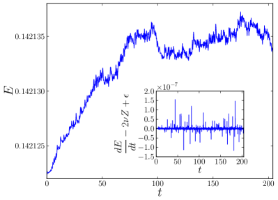
Under the procedure described above, the typical evolution of the energy in a numerical simulation is shown in Fig. 2. The energy starts from the value corresponding to the fluid at rest (i.e., all the energy is the potential energy associated with the equilibrium height ). The total energy then grows under the action of the external mechanical forcing, and after the system reaches a turbulent steady state in which the energy fluctuates around a mean value, and in which the energy injection and dissipation are equilibrated on the average. Even though pseudospectral methods are known to introduce no numerical dissipation, in the inset of Fig. 2 we also show explicitly that the energy balance (Eq. (28)) is satisfied with an error of order , which remains stable and does not grow even after integrating for very long times.
To ensure that the flow in the simulations remained shallow for all excited wavenumbers, we enforced the following condition
| (30) |
where is, as already mentioned, the shortest wavelength resolved by the code in virtue of the condition given by Eq. (26).
IV Results
IV.1 Description and classification of the simulations
The spectral behavior of the flow in the simulations depends on the external parameters. We can independently control the height of the fluid at rest , the viscosity , the gravity acceleration , the amplitude of the forcing , the range of wavenumbers in which the force is applied, and the linear resolution . However, all these parameters can be reduced to a smaller set of dimensionless controlling parameters.
One of these parameters is the Froude number
| (31) |
which measures the ratio of inertia to gravity acceleration in the momentum equation, and where is the r.m.s. velocity.
Another dimensionless parameter is the non-linear number, . In order to be in the regime of weak turbulence, nonlinearities should be small. The effect of nonlinearities can be measured by how large perturbations in are compared to , so we define as
| (32) |
where is the r.m.s. value of .
The two remaining dimensionless numbers are the Reynolds number,
| (33) |
where is the forcing scale (defined as ), and what we will call the dispersivity, , defined as
| (34) |
following Eq. (30). This last number, only relevant for the Boussinesq model, measures how strong the dispersion is at the smallest scales, and for sufficiently small we can expect the solutions of the Boussinesq model to converge to the solutions of the shallow water model. In fact, it is easy to show from the weak turbulence spectrum in Eq. (25) that when the maximum resolved wavenumber is associated with the dissipation wavenumber , then
| (35) |
Decreasing below the value given by this relation should result in negligible dispersion at all resolved wavenumbers. Note that the level of dispersion in a given Boussinesq run depends on the wavenumber, and actually quantifies the strongest possible dispersion at the smallest scales in the flow.
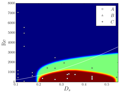
By qualitatively assessing each run, we can classify them into three sets, , , and . In tables 1, 2, 3 the different dimensionless parameters, along with a few other useful quantities, are given for each simulation in each set, respectively. How and why these three sets differ from each other will be made clear in the following sections, when we discuss the actual results. But, for the moment, it is fruitful to analyze the behavior of the values of Re and in each set, so as to keep them in mind for later on.
The values of Re and for all the Boussinessq runs are shown in Fig. 3. As a reference, Fig. 3 also shows the curve given by Eq. (35) with estimated from the values from the simulations in set . Points below that curve are expected to have non-negligible dispersion. Runs in set have relatively small Re (), and varying between and . In other words, dispersion effects in runs in set are important. Runs in set have smaller values of (except for one run with , all other runs have ), and Re varying between and . These runs have small or negligible dispersion, and note all the SW runs we performed belong to this set. The runs in set are intermediate between these two regimes.
Finally, although the mechanical forcing we use introduces no vorticity in the horizontal velocity field, some vorticity is spontaneously generated as the flow evolves. This is probably also the case in experiments. In order to quantify the presence of vortical structures, we calculated the ratio of vorticity to divergence in the horizontal velocity field
| (36) |
which turns out to be for all simulations. As a result, although the flow is not perfectly irrotational, the amplitude of vortical modes is small compared with the amplitude of modes associated with the waves.
IV.2 Energy spectra
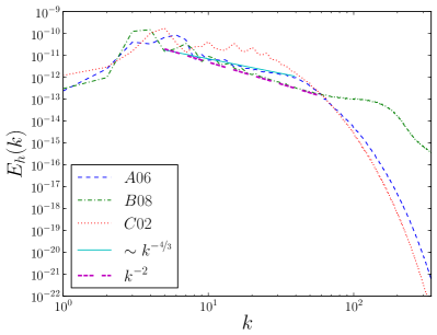
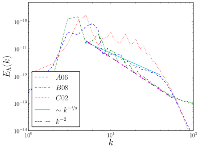
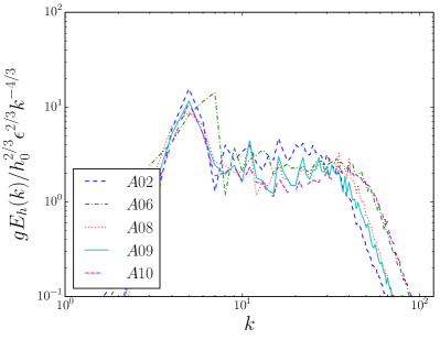
The power spectrum of (proportional to the spectrum of the potential energy) as a function of the wave number is shown in Fig. 4 for runs , , and . Figure 5 shows a close-up of the same spectrum in the inertial range. It is clearly seen that runs in each set show a different behavior. On the one hand, the run belonging to group has an inertial range compatible with scaling, which is the spectra predicted by weak turbulence. On the other hand, the run in set displays an inertial range compatible with dependency. While this spectrum is not predicted by weak turbulence, it was observed before in experiments and observations Kaihatu et al. (2007). The run in group shows a shallower spectrum with no clear inertial range. We think of runs in this set as transitional between the other two.
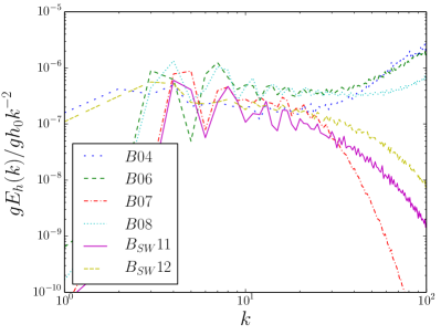
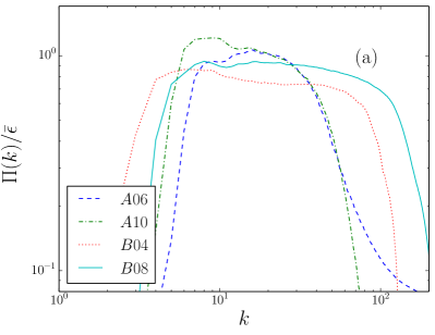
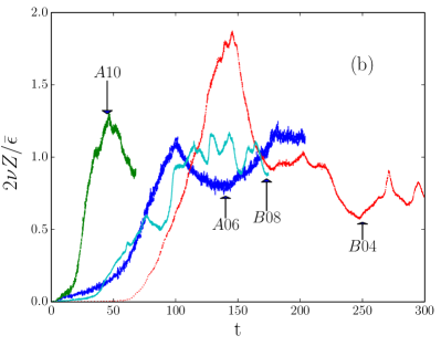
The other runs in sets , , and show similar power spectra for . To show this, we present the compensated spectra for the simulations in sets and in Figs. 6 and 7 respectively (simulations from set do not have a clearly defined inertial range and are therefore not shown). The simulations from set are compensated by (which is the weak turbulence spectrum, using the height of the fluid column at rest, , and the energy injection rate, , as prefactors), while the ones in set are compensated by (more details on the choice of the prefactor are given below). These figures indicate that, within statistical uncertainties, all spectra in each set collapse to the same power laws, and that the simulations are well converged from the point of view of spatial resolution. Furthermore, we verified that the energy flux is approximately constant in the scales corresponding to the inertial range of each simulation. Within the limitations of spatial resolution and the drop in the flux for large wavenumbers caused by viscous dissipation, an incipient inertial range can be identified in the flux of each simulation. Figure 8 shows the instantaneous energy flux (normalized by the energy injection rate averaged over time) as a function of for several simulations in sets and . The energy flux was calculated from the energy balance equation in Fourier space, as is usually done for turbulent flows. Figure 8 also shows the normalized energy dissipation rate as a function of time (equivalent to the normalized energy flux as a function of time) for the same runs, to show that this quantity fluctuates around a mean value in the turbulent steady state.
The kinetic energy spectrum is similar to the power spectrum of , and in approximate equipartition with the potential energy spectrum once the system reaches a turbulent steady state. It is interesting to analyse this in the light of the values of the dimensionless parameters in the runs as shown in Fig. 3. As was explained in the previous section, set corresponds to runs with lower Reynolds number and larger dispersivity (, and varying between and ). As a result, these runs can be expected to display weak turbulence behavior as described in Section II.5, because the nonlinearities are not so large as to break the weak turbulence hypothesis Onorato et al. (2009), and the dispersion is not so low as to render the higher order terms of Eq. (14) negligible (in which case four-wave interactions would no longer be dominant, and the hypothesis used to derive Eq. (24) would not be satisfied). In contrast, runs in set have larger Re and lower (except for one run with , all other runs have , and Re varying between and ). In this case dispersion is smaller or negligible, while nonlinearities can be expected to be larger, two conditions that render the derivation resulting in Eq. (25) invalid.
Moreover, the spectra observed in the simulations in set include those runs that solve the SW model. Therefore, these spectra cannot be explained by weak turbulence, as SW simulations have no dispersion and the arguments in Section II.5 do not apply. Also, note that in the non-dispersive limit, for constant and fixed , the SW equations can be reduced to the two-dimensional Burgers equations, which amplify negative field gradients by strong nonlinearities resulting in sharp fronts in the velocity. Such a field would actually have a spectrum (note this is also the behavior expected for two-dimensional non-dispersive acoustic turbulence L’vov et al. (1997), that also develops sharp fronts). The spectrum can be obtained from dimensional analysis and the scaling that results for the energy is equivalent to Phillips’ spectrum Phillips (1958) but in two dimensions. In the presence of strong nonlinearities, we can assume that the nonlinear and gravity terms are of the same order,
| (37) |
It is also reasonable to assume that the kinetic and potential energies will be of the same order (i.e., in equipartition) in the turbulent steady state. This implies that is the only dimensional constant the spectra can depend on. This is precisely how Phillips derived his spectrum.
With these assumptions in mind, it is easy to obtain the observed spectra. The energy spectrum has units of energy in the fluid column per unit surface per wavenumber, , and assuming , from dimensional analysis the only possible solution is
| (38) |
The independence of the spectrum on the energy injection rate suggests that the energy transfer between the different scales must take place by a mechanism such as wave breaking in the case of Phillips’ spectrum, which occurs when the slope of the surface is larger than a critical value, or by nonlinear wave steepening in our case (which is finally regularized by the viscosity). Such a mechanism is independent of the power injected by external forces. Of course, this can only hold in a region of parameter space, as in the presence of weak forcing and dispersion, the solution in Eq. (25) is expected instead.
In summary, based on the numerical results, the simulations with weaker forcing and higher dispersion develop a spectrum compatible with the predictions from weak turbulence theory, while the runs with stronger forcing or with less (or no) dispersion are compatible with dimensional analysis based on strong turbulence arguments.
IV.3 Comparison between SW and BQ models
All simulations of the SW model belong to set , as that is the set of runs that has negligible or no dispersion. All other sets have moderate dispersion, and as a result the flow dynamics cannot be captured by the SW model. Note that runs in set are also the runs with an inertial range compatible with scaling. However, the BQ and SW runs in set are not identical. In this subsection we discuss the differences between these runs.
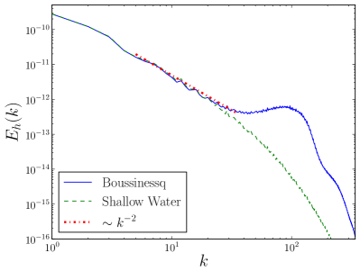
As an example of two runs with and without dispersive effects, the power spectra of for runs and are shown in Fig. 9. Both simulations have the same parameters, except for the viscosity which is larger in the simulation using the SW model. At small wavenumbers, where dispersion is negligible, the spectra of the BQ and SW models coincides. For wavenumbers larger than , dispersion in the BQ model becomes important and a bump (an accumulation of energy at small scales) develops. This accumulation in the BQ model results in an increased dissipation (as dissipation is proportional to ), thus allowing us to simulate the system with smaller viscosity. This difference at large wavenumbers is the most distinct feature in the two spectra in Fig. 9.
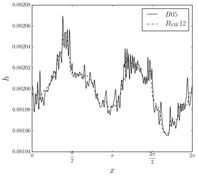
As a result of the extra power at larger wavenumbers, dispersion in the BQ model results in more prominent small scale features, and in rapidly varying waves. As an example, Fig. 10 shows a transversal cut in the elevation field for runs and . The cuts are taken at the same place and at the same time in both runs. Even though both simulations have the same behavior at large scales, at short length scales the BQ model presents fast fluctuations. These fluctuations are well resolved (the cut corresponds to grid points), and there is no indication that resolution is insufficient to resolve the sharp gradients. In the BQ model, while the large scales may correspond to a shallow flow, as long as there is enough scale separation, there will always be a wavenumber where the finite depth effects can be seen. Thus, the Boussinesq equations provide an interesting model to study weakly dispersive waves.
Regarding the accumulation of energy that leads to a flatter spectrum for high wavenumbers in some of the BQ simulations (for several runs in set as can be seen in Fig. 7, but specially in the runs in set ), such an accumulation has been observed before in turbulent flows. As mentioned above, we verified that this accumulation is not the result of insufficient resolution (e.g., by comparing the runs with different grid points ). The accumulation of energy in the spectrum near the dissipative range is often termed “bottleneck”, and bottlenecks can have dissipative Falkovich (1994) or dispersive Graham et al. (2007); Krstulovic and Brachet (2011) origins. In the former case, the accumulation results from the viscous damping of the triads at small scales, resulting in a decrease of the energy flux. Such a viscous bottleneck should be visible also in the non-dispersive simulations, and its absence in those runs indicates a dispersive origin. In the latter case, the bottleneck arises from the increasingly harder to satisfy resonant condition for the wave frequencies, as the waves become faster at smaller scales. Models with a field filtered by the Helmholtz operator (as is the case for the BQ model, see Eq. 15) tend to develop a bottleneck (see Graham et al. (2007) for a detailed description of its origin). A qualitative way to explain the tendency towards a flatter spectrum in the BQ model can be obtained by assuming that dispersion is strong enough for the dispersive term to be balanced with the buoyancy and with the non-linear terms in the BQ equations (i.e., all terms are of the same order). Then the energy spectra can depend only on both and , and a possible solution is . A detailed study of the origin of this bottleneck is left for future work.
At this point it is worth pointing out that when and dispersion becomes too strong, the Boussinesq approximation breaks down as more terms in the Taylor expansion in Eq. (11) should be preserved. As a result, the Boussinesq approximation is useful as long as at the smallest excited scales in the system. On the other hand, from Fig. 3, if the behavior of the system in the inertial range is that of a shallow water flow for all Reynolds numbers studied.
IV.4 Time-resolved spectra and non-linear dispersion relations
Wavenumber spectra, as the spectra discussed so far, give information of how energy is distributed in spatial scales, but do not provide a quantitative estimate of how much energy in the system is associated with wave motions. A frequency spectrum is often obtained from the wavenumber spectrum using the dispersion relation (or vice versa). However, in systems that can sustain both wave and vortical motions there is no clear justification to use the dispersion relation to go from one spectrum to the other.
A quantification of the amount of energy in waves, and on whether non-linear effects change the dispersion relation of the system from the linear one, can be directly obtained from the frequency and wavenumber spectrum without any assumption. The spectrum can be computed by storing the Fourier coefficients of the height as a function of time (as well as the Fourier coefficients of the velocity field), then computing the Fourier transform in time, and finally computing the isotropic power spectrum by averaging in the -plane. To this end, several large-scale wave periods and turnover times must be stored (to resolve the slowest frequencies in the system), with sufficient time resolution to resolve the fastest frequencies. In the analysis we show below, time series spanning at least three periods of the slowest waves were used, and with time resolution .
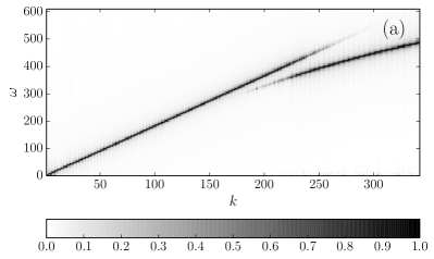
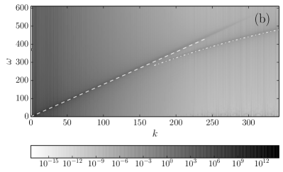
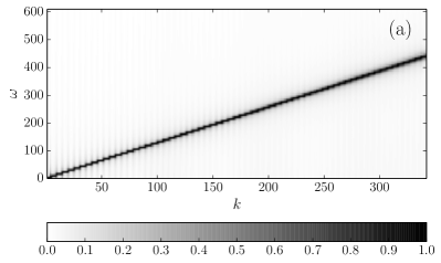
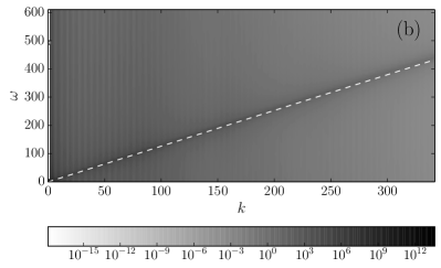
Figures 11 and 12 show the power spectrum of the flow height for simulations and respectively. The linear dispersion relations for shallow water flows (Eq. 4) and for Boussinesq flows (Eq. 14) are also shown as references, using the parameters from each run. Note both runs present an energy accumulation near the dispersion relation. This indicates most of the energy is in the waves, and remains there as time evolves. As we are not solving the equations for a potential flow, and the system can develop vortical motions, this tells us that the non-linear energy transfer is mostly done between waves, and that the energy injected at large scales in wave motions is mostly transferred towards wave motions at smaller scales and faster frequencies. This is needed for weak turbulence to hold, but is also observed in run that has a spectrum compatible with strong turbulence phenomenological arguments. There is also a turbulent broadening of the dispersion relation, also visible in cross sections of the spectrum at different wavenumbers in Fig. 13. From this broadening, the characteristic time of non-linear wave interactions can be obtained, as was done in Miquel and Mordant (2011).

Some of the most important results in this paper are associated with these two figures. First, note that in run most of the energy is concentrated near a dispersion relation that, as dispersion is negligible, corresponds in practice to the non-dispersive shallow-water case (Eq. 4). All runs in set have the same spectral behavior in , and confirm that the spectrum is observed when dispersion is negligible or absent (i.e., when the flow is sufficiently shallow). Second, note that the spectrum in run presents clear signs of dispersive effects (i.e., most of the energy for large enough is concentrated over a curve that deviates from a linear relation between and ), and this run displays a scaling in compatible with the weak turbulence prediction . This behavior was observed in the other runs in set .
However, for runs in set presents yet another interesting feature. As expected, for small the dispersion is negligible and the energy is concentrated over a straight line in space. At large , as already mentioned, the effective dispersion relation is compatible with that of the linearized Boussinesq equations. But at intermediate wavenumbers two branches of the dispersion relation can be observed, one that is compatible with non-dispersive waves and another compatible with dispersive waves. When both branches are present, their amplitudes are of the same order, as can be seen in Fig. 13.
At first sight, the existence of these two branches could be attributed to bound waves. Bound waves are small amplitude waves which are bounded to a parent wave of larger amplitude. The waves are bounded in the sense that they follow the parent wave, i.e., they travel with the same phase velocity as the parent, and thus they follow an anomalous dispersion relation (see, e.g., a discussion of bound waves in the context of gravito-capillary waves in Longuet-Higgins (1963); Herbert et al. (2010)). The condition that they have the same phase velocity as the parent wave implies that they must follow a modified dispersion relation which verifies , where is the wavenumber of the parent wave. Bound waves result in multiple branches in the spectrum (and in multiple peaks in the frequency spectrum). Indeed, it is easy to show that for , , these multiple branches satisfy
| (39) |
(see, e.g., the discussion in Herbert et al. (2010)). Extending the analysis in Herbert et al. (2010) to our case, bound waves in the BQ model should satisfy the following dispersion relation,
| (40) |
which verifies Eq. (39). However, the second branch in Fig. 12 cannot be described by this dispersion relation for any value of up to 4, and thus they are not bound waves in the sense often used in oceanography.
Another explanation for the existence of these two branches can be given by keeping in mind that at intermediate wavenumbers slight variations in the fluid depth may trigger a transition in the waves from dispersive to non-dispersive (as the level of dispersion depends on the product of the wavenumber with the surface height). Indeed, in the turbulent flow there are waves with short wavelengths which ride over long ones, that have a larger amplitude. For sufficient scale separation, the fast waves see an effective depth that can be larger or smaller than depending on whether the wave is on a crest or a valley of the slow wave, generating in one case dispersive waves, and in the other non-dispersive waves.
We can estimate the variation in the effective dispersion at a given wavenumber . In simulation , and the longer waves have an amplitude (as can be estimated, e.g., from the maximum value of the power spectrum of ). From the system dispersion relation,
| (41) |
dispersion is controlled by the amplitude of the term. Assuming that fast waves experience an effective depth (where the sign depends on whether they are on a valley or a crest), the variation in the dispersion is proportional to the difference between and . So, for this simulation, the variation is around , and when multiplied by , it is sufficient to explain the two branches in for between and .
IV.5 Time frequency energy spectra
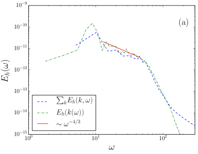
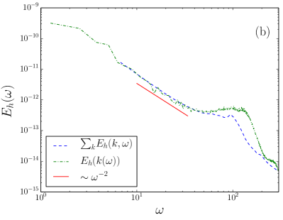
From the spectra in Figs. 11 and 12 the frequency spectrum can be easily obtained, simply by summing over all wavenumbers,
| (42) |
As already mentioned, in experiments and simulations is sometimes estimated instead from by using the dispersion relation in the form . Figure 14 shows the power spectrum of as a function of for simulations and . In both cases, the spectrum was calculated explicitly using Eq. (42), and also estimated using the dispersion relation. For each run, the two spectra show a very good agreement, which can be expected as most of the energy is in the waves. The behavior of the inertial range in each run is also in good agreement with the one found previously for in Sec. IV.2.
IV.6 Probability density functions
We calculated the probability density function (PDF) of the free surface height for different simulations. Figure 15 shows the PDF of for run , where is the standard deviation of the surface height. The probability distribution is asymmetric, with a larger probability of measuring large values of than of small values. The shape can be adjusted by two distributions: We consider a skewed normal distribution Azzalini (1985),
| (43) |
where is the so-called scale parameter (associated with the variance of the distribution), is the location parameter (associated with the mean value), is the shape parameter (associated with the skewness), and
| (44) | ||||
| (45) |
We also consider a Tayfun distribution
| (46) |
with and where is the mean steepness of the wavesTayfun (1980).
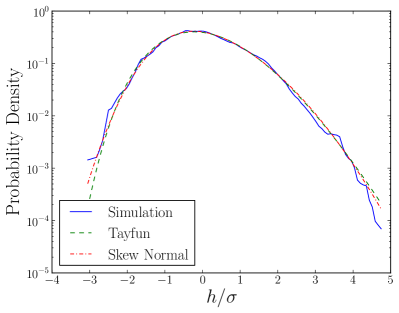
For run , and from a Maximum Likelihood Estimation method for the skewed normal distribution, the location parameter is , the scale parameter is , and the shape parameter is . For the same run, and for the Tayfun distribution, the mean steepness of the waves is . This latter value is more relevant as the Tayfun distribution is often used in oceanography and in experiments of surface waves. In this context, it is interesting to point out that experiments in Falcon and Laroche (2011) found similar values for .
This behavior (a PDF of described correctly by both a skewed normal distribution and a Tayfun distribution with asymmetry to the left) was observed in all simulations, no matter what set they belonged to.
V Conclusions
We studied wave turbulence in shallow water flows in numerical simulations using the shallow water and Boussinesq models. The equations were solved using grids up to points, and the parameters were varied to study different regimes, including regimes with larger and smaller Reynolds number, and larger and smaller dispersion, while keeping the Froude number approximately the same. We summarize below the main conclusions following the same ordering as in the introduction:
(a) As in previous experimental and observational studies Smith and Vincent (2003); Kaihatu et al. (2007), we found that the flows can be classified in different sets depending on the value of the Reynolds number (i.e., on the strength of the nonlinearities) and on the level of dispersion (associated with the fluid depth). A first set () has smaller Reynolds numbers and stronger dispersion, a second set () has larger Reynolds numbers and weaker or negligible dispersion, and a third set of runs seems to be transitional between the two.
(b) Runs in sets and have different power spectra of the surface height. Runs in set , with stronger dispersion, present a spectrum compatible (within statistical uncertainties) with . This is the spectrum predicted by weak turbulence theory for the Boussinesq equations Onorato et al. (2009). Runs in set with negligible or zero dispersion (i.e., for a shallower flow) show a spectrum compatible within error bars with . This spectrum can be obtained from phenomenological arguments coming from strong turbulence Phillips (1958). The runs in set have no discernible inertial range.
(c) The Boussinesq (dispersive) model tends to develop more power in waves with short wavelengths than the shallow water model. This is associated with the development of a bottleneck for large wavenumbers in the energy spectrum.
(d) Inspection of the wave and frequency spectrum confirms that most of the energy is in the waves in all the simulations. In runs in set , most of the energy is concentrated in the vicinity the linear dispersion relation for shallow water waves, which are non-dispersive. In runs in set , the resulting non-linear dispersion relation obtained from has two branches: one that corresponds to non-dispersive waves, and another corresponding to dispersive waves. The two branches can be explained as the result of the superposition of rapidly varying waves which ride over slowly varying waves, the latter with sufficient amplitude to change whether the former see a shallower or deeper fluid.
(e) Independently of the differences between the runs, the probability distribution functions of for the runs in all sets is asymmetric, with larger probabilities of finding larger values of than smaller values. The probability distribution functions can be approximated by both a skewed normal distribution and a Tayfun distribution Tayfun (1980). In the latter case, the only parameter of the distribution, the mean steepness of the waves, has values compatible with those found in observations and experimental studies (see Falcon and Laroche (2011)). The obtained probability density functions also indicate limitations in the hypothesis of Gaussianity of the fields assumed in early theories of weak turbulence. However, extensions of the theory to allow for non-Gaussian distributions exist and can be found for example in Choi et al. (2004) and Lvov and Nazarenko (2004); Choi et al. (2005).
All the results presented here were obtained solving numerically equations that do not assume that the flow is inviscid or irrotational, and with realistic terms for the viscous dissipation. We believe this approach can be useful to compare with experiments, as in experiments vorticity can develop in the flow, and viscosity cannot be neglected.
Acknowledgements.
The authors would like to thank Prof. Oliver Buhler and the anonymous referees for their useful comments. The authors acknowledge support from grants No. PIP 11220090100825, UBACYT 20020110200359, and PICT 2011-1529 and 2011-1626. PDM and PJC acknowledge support from the Carrera del Investigador Científico of CONICET, and PCdL acknowledges support from CONICET.References
- Iafrati et al. (2013) A. Iafrati, A. Babanin, and M. Onorato, Physical Review Letters 110, 184504 (2013).
- D’Asaro et al. (2011) E. D’Asaro, C. Lee, L. Rainville, R. Harcourt, and L. Thomas, Science 332, 318 (2011).
- Ivey et al. (2008) G. Ivey, K. Winters, and J. Koseff, Annual Review of Fluid Mechanics 40, 169 (2008).
- Rose et al. (2010) K. A. Rose, E. L. Sikes, T. P. Guilderson, P. Shane, T. M. Hill, R. Zahn, and H. J. Spero, Nature 466, 1093 (2010).
- Cavaleri et al. (2012) L. Cavaleri, B. Fox-Kemper, and M. Hemer, Bulletin of the American Meteorological Society 93, 1651 (2012).
- Falnes (2007) J. Falnes, Marine Structures 20, 185 (2007).
- Hasselmann (1962) K. Hasselmann, Journal of Fluid Mechanics 12, 481 (1962).
- Hasselmann (1963a) K. Hasselmann, Journal of Fluid Mechanics 15, 385 (1963a).
- Hasselmann (1963b) K. Hasselmann, Journal of Fluid Mechanics 15, 273 (1963b).
- Zakharov et al. (1992) V. E. Zakharov, V. S. Lvov, and G. Falkovic, Kolmogorov Spectra of Turbulence I – Wave Turbulence (Springer, Berlin [u.a.], 1992).
- Newell and Rumpf (2011) A. C. Newell and B. Rumpf, Annual Review of Fluid Mechanics 43, 59 (2011).
- Nazarenko (2011) S. Nazarenko, Wave Turbulence, 2011th ed. (Springer, 2011).
- Düring et al. (2006) G. Düring, C. Josserand, and S. Rica, Physical review letters 97, 025503 (2006).
- Galtier (2003) S. Galtier, Physical Review E 68, 015301 (2003).
- Galtier et al. (2000) S. Galtier, S. V. Nazarenko, A. C. Newell, and A. Pouquet, Journal of Plasma Physics 63, 447–488 (2000).
- Schekochihin et al. (2012) A. A. Schekochihin, S. V. Nazarenko, and T. A. Yousef, Physical Review E 85, 036406 (2012).
- Deike et al. (2012) L. Deike, M. Berhanu, and E. Falcon, Physical Review E 85, 066311 (2012).
- Falcón et al. (2009) C. Falcón, E. Falcon, U. Bortolozzo, and S. Fauve, EPL (Europhysics Letters) 86, 14002 (2009).
- Kolmakov et al. (2004) G. V. Kolmakov, A. A. Levchenko, M. Y. Brazhnikov, L. P. Mezhov-Deglin, A. N. Silchenko, and P. V. E. McClintock, Physical review letters 93, 074501 (2004).
- Cobelli et al. (2011) P. Cobelli, A. Przadka, P. Petitjeans, G. Lagubeau, V. Pagneux, and A. Maurel, Physical Review Letters 107, 214503 (2011).
- Mordant (2008) N. Mordant, Physical review letters 100, 234505 (2008).
- Boudaoud et al. (2008) A. Boudaoud, O. Cadot, B. Odille, and C. Touzé, Physical Review Letters 100, 234504 (2008).
- Cobelli et al. (2009) P. Cobelli, P. Petitjeans, A. Maurel, V. Pagneux, and N. Mordant, Physical Review Letters 103, 204301 (2009).
- Leerink et al. (2012) S. Leerink, V. V. Bulanin, A. D. Gurchenko, E. Z. Gusakov, J. A. Heikkinen, S. J. Janhunen, S. I. Lashkul, A. B. Altukhov, L. A. Esipov, M. Y. Kantor, T. P. Kiviniemi, T. Korpilo, D. V. Kuprienko, and A. V. Petrov, Physical Review Letters 109, 165001 (2012).
- Mininni and Pouquet (2007) P. D. Mininni and A. Pouquet, Physical Review Letters 99, 254502 (2007).
- Chen et al. (2005) Q. Chen, S. Chen, G. L. Eyink, and D. Holm, Journal of Fluid Mechanics 542, 139–164 (2005).
- Phillips (1958) O. M. Phillips, Journal of Fluid Mechanics 4, 426 (1958).
- Toba (1973) Y. Toba, Journal of the Oceanographical Society of Japan 29, 209 (1973).
- Donelan et al. (1985) M. A. Donelan, J. Hamilton, and W. H. Hui, Philosophical Transactions of the Royal Society of London. Series A, Mathematical and Physical Sciences 315, 509 (1985).
- Badulin et al. (2007) S. I. Badulin, A. V. Babanin, V. E. Zakharov, and D. Resio, Journal of Fluid Mechanics 591 (2007).
- Phillips (1985) O. M. Phillips, Journal of Fluid Mechanics 156, 505 (1985).
- Korotkevich (2008) A. Korotkevich, Physical Review Letters 101 (2008).
- Zakharov (1999) V. Zakharov, European journal of mechanics. B, Fluids 18, 327–344 (1999).
- Onorato et al. (2009) M. Onorato, A. R. Osborne, P. A. E. M. Janssen, and D. Resio, Journal of Fluid Mechanics 618, 263 (2009).
- Smith and Vincent (2003) J. M. K. Smith and C. L. Vincent, Journal of geophysical research 108, 3366 (2003).
- Kaihatu et al. (2007) J. M. Kaihatu, J. Veeramony, K. L. Edwards, and J. T. Kirby, Journal of geophysical research 112, C06016 (2007).
- Falcon and Laroche (2011) E. Falcon and C. Laroche, EPL (Europhysics Letters) 95, 34003 (2011).
- Landau and Lifshitz (2004) L. D. Landau and E. M. Lifshitz, Fluid mechanics (Elsevier/Butterworth-Heinemann, Amsterdam, 2004).
- Pedlosky (1987) J. Pedlosky, Geophysical fluid dynamics, 2nd ed. (Springer-Verlag, New York, 1987).
- Whitham (1974) G. B. Whitham, Linear and nonlinear waves (Wiley, New York [u.a.], 1974).
- Dyachenko et al. (2004) A. I. Dyachenko, A. O. Korotkevich, and V. E. Zakharov, Physical Review Letters 92 (2004).
- Yokoyama (2004) N. Yokoyama, Journal of Fluid Mechanics 501, 169 (2004).
- Marche (2007) F. Marche, European Journal of Mechanics - B/Fluids 26, 49 (2007).
- Choi (1995) W. Choi, Journal of Fluid Mechanics 295, 381 (1995).
- Mininni et al. (2005a) P. D. Mininni, D. C. Montgomery, and A. G. Pouquet, Physics of Fluids 17, 035112 (2005a).
- Mininni et al. (2005b) P. D. Mininni, D. C. Montgomery, and A. Pouquet, Physical Review E 71, 046304 (2005b).
- Foias et al. (2001) C. Foias, D. D. Holm, and E. S. Titi, Physica D Nonlinear Phenomena 152-153, 505 (2001).
- Camassa and Holm (1993) R. Camassa and D. D. Holm, Physical Review Letters 71, 1661 (1993).
- Graham et al. (2007) J. P. Graham, D. D. Holm, P. D. Mininni, and A. Pouquet, Physical Review E 76, 056310 (2007).
- L’vov et al. (1997) V. S. L’vov, Y. L’vov, A. C. Newell, and V. Zakharov, Physical Review E 56, 390–405 (1997).
- Gómez et al. (2005a) D. O. Gómez, P. D. Mininni, and P. Dmitruk, Advances in Space Research 35, 899 (2005a).
- Gómez et al. (2005b) D. O. Gómez, P. D. Mininni, and P. Dmitruk, Physica Scripta , 123 (2005b).
- Mininni et al. (2011) P. Mininni, D. Rosenberg, R. Reddy, and A. Pouquet, Parallel Computing 37, 316 (2011).
- Canuto et al. (1988) C. Canuto, M. Hussaini, A. Quarteroni, and T. Zang, Spectral methods in fluid dynamics, corr. 3rd print ed. (Springer-Verlag, Berlin ; New York, 1988).
- Falkovich (1994) G. Falkovich, Physics of Fluids 6, 1411 (1994).
- Krstulovic and Brachet (2011) G. Krstulovic and M. Brachet, Physical Review Letters 106 (2011).
- Miquel and Mordant (2011) B. Miquel and N. Mordant, Physical Review E 84 (2011).
- Longuet-Higgins (1963) M. S. Longuet-Higgins, Journal of Fluid Mechanics 16, 138 (1963).
- Herbert et al. (2010) E. Herbert, N. Mordant, and E. Falcon, Physical Review Letters 105, 144502 (2010).
- Azzalini (1985) A. Azzalini, Scandinavian Journal of Statists 12, 171 (1985).
- Tayfun (1980) M. A. Tayfun, Journal of Geophysical Research: Oceans 85, 1548–1552 (1980).
- Choi et al. (2004) Y. Choi, Y. V. Lvov, and S. Nazarenko, Physics Letters A 332, 230 (2004).
- Lvov and Nazarenko (2004) Y. Lvov and S. Nazarenko, Physical Review E 69 (2004).
- Choi et al. (2005) Y. Choi, Y. V. Lvov, and S. Nazarenko, Physica D: Nonlinear Phenomena 201, 121 (2005).