Abstract

Diffusion processes have been applied with great success to model the dynamics of large populations throughout science, in particular biology. One advantage is that they bridge two different scales: the microscopic and the macroscopic one. Diffusion is a mathematical idealisation, however: it assumes vanishingly small state changes at the microscopic level. In real biological systems this is often not the case. The differential Chapman-Kolmogorov equation is more appropriate to model population dynamics that is not well described by drift and diffusion alone.

Here, the method of characteristics is used to transform deterministic dynamics away and find a coordinate frame where this equation reduces to a Master equation. There is no longer a drift term, and solution methods there are insensitive to density gradients, making the method suitable for jump processes with arbitrary jump sizes. Moreover, its solution is universal: it no longer depends explicitly on the deterministic system.

We demonstrate the technique on simple models of neuronal populations. Surprisingly, it is suitable for fast neural dynamics, even though in the new coordinate frame state space may expand rapidly towards infinity. We demonstrate universality: the method is applicable to any one dimensional neural model and show this on populations of leaky- and quadratic-integrate-and-fire neurons. In the diffusive limit, excellent approximations of Fokker-Planck equations are achieved. Nothing in the approach is particular to neuroscience, and the neural models are simple enough to serve as an example of dynamical systems that demonstrates the method.

Author Summary

Biological systems stand out by their complexity and multi-scale interactions. Modeling techniques that can explain the behavior of systems - the macroscopic level - in terms of their individual components - the microscopic level - are very valuable. Diffusion models do that, so, unsurprisingly, they pervade biology. One key assumption underlying the validity of the diffusion approach is that state changes of individuals are minuscule. In real biological systems this can often not be justified. The method presented here dispenses with the assumption and broadens the application range of population modelling considerably. Moreover, the method reduces the mathematically difficult problem of solving a partial differential equation to a simpler one: understanding the noise process that gave rise to it.

We demonstrate the approach on neuronal populations. We envisage that the study of networks of such populations will elucidate brain function, as large-scale networks can be simulated with unprecedented realistic neural dynamics. This may help explain imaging signals, which after all are the observable collective signal of large groups of neurons, or it may help researchers to develop their ideas on neural coding. We also expect that the technique will find broad application outside of neuroscience and biology, in particular in finance.

Introduction

Diffusion models are of crucial importance to biological modeling; literally, text books have been filled on the subject, e.g. [1, 2]. The application domain is enormous: fluid dynamics, chemotaxis [3], animal population movement [4, 5], neural populations e.g. [6, 7, 8, 9, 10, 11, 12, 13, 14, 15, 16, 17] are just a few examples (see [18] for a recent review and further references). Diffusion models allow an understanding of group behaviour in terms of that of its constituents, i.e. they link macroscopic and microscopic behaviour. In general diffusion models emerge as follows: microscopic deterministic laws describing individual behavior in the absence of interactions are determined. Interactions among individuals and between individuals and the outside world are described by a stochastic process (’noise’). Diffusion arises if one assumes that changes in the microscopic state as a consequence of an interaction are vanishingly small. Sometimes, this assumption is well justified: for example, in Brownian motion these interactions are due to the collisions of individual molecules, interactions that are indeed minuscule compared to the macroscopic state. Often, this assumption is not appropriate, but made in order to use the familiar mathematical machinery of diffusion equations. For example, in computational neuroscience the diffusion approximation hinges on the assumption that synaptic efficacies - a measure for how strongly neurons influence each other - are small. This is simply not the case in many brain areas, e.g. [19], and leads to sizable corrections to diffusion results [20]. Nevertheless, the diffusion approximation predominates in computational neuroscience. Given the widespread distribution of diffusion models in biology, it stands to reason that this situation is common.

Experience from computational neuroscience [20] and finance - a field that has put considerable effort into understanding jump diffusion equations e.g. [21, 22, 23] - has shown that results valid beyond the diffusion limit are very hard to obtain, limited to a specific study and often require a perturbation approach [20]. Due to their nature, jump diffusion processes may lead to very jagged, locally discontinuous probability density profiles [24]. For this reason numerical solution schemes that are well established for diffusion processes may be unsuitable for finite size jumps. Some solution schemes are applicable for finite jumps if it can be assumed that the underlying density profile is smooth. Brennan and Schwartz [25] demonstrated that an implicit scheme for solving the Black-Scholes equation is equivalent to a generalized jump process. The assumption must be justified, however. In contrast, the method presented here makes no assumptions about the structure of the underlying structure of the density profile at all. Below, we will present an example that can be easily modeled by the method presented here, but where we are not aware of more conventional discretization schemes that would apply.

Standard text books such as [24, 26] demonstrate how deterministic laws of motion for individuals and a Master equation describing the noise process under consideration can be combined. This results in the so-called differential Chapman-Kolmogorov equation, a partial integro-differential equation in probability density (it is derived in the context of neuronal populations in “Methods: Derivation of the population density equation”). When the assumption is made that the transitions due to the stochastic processes induce very small state transitions, this equation reduces to a partial differential equation of the Fokker-Planck type [24, 26]. Diffusion models ultimately derive from this equation. Clearly, a solution method for the Chapman-Kolmogorov equation is highly valuable: it would still allow the study of diffusion processes, but also processes with large jumps. Below, we will give an example of the gradual breakdown of diffusion. This opens up an important application area: it will be possible to re-examine results already obtained in the diffusion limit and to investigate the consequences of finite jump sizes.

Many expositions immediately proceed to the diffusion regime. Here we follow a radically different approach: we use the method of characteristics to define a coordinate frame that co-moves with the flow of the deterministic system. In this frame the differential Chapman-Kolmogorov equation reduces to the Master equation of the stochastic process under consideration. This approach neatly sidesteps the need for solving a partial (integro-) differential equation as the Master equation is a set of ordinary differential equations, and can be solved by relatively simple numerical methods.

This simplicity comes at a price, however: the probability density is represented in an interval that is moving with respect to the new coordinate frame. How this interval behaves becomes dependent on the topology of the flow of the deterministic system. We will illustrate the problem on two neuron models that represent two ends of the dynamic spectrum. Leaky-integrate-and-fire neurons have slow underlying deterministic dynamics. Quadratic-integrate-and-fire neurons model the rapid onset of a spike. The dynamics is so fast that the original interval representing the probability density profile moves to infinity in finite time in the new coordinate frame.

We find that these neural models are a demonstration of the broad applicability of the technique. Not only are they simple examples of dynamical systems that can easily be understood without a background in computational neuroscience. They also provide boundary conditions that any good solution method must be able to handle: absorbing boundaries. In general neurons spike and then return to pre-spike conditions. In one dimensional neural models this is simulated by resetting the neuronal state as soon as an absorbing boundary (the ’threshold’) is reached. The reintroduction of a neuron once it has hit the threshold (a ’reset’) is particular to neural systems. It is a marked difference from financial derivatives - as options become worthless after their expiration date - and one reason why results from finance do not carry over to neuroscience despite similarities.

The method is manifestly stable, and the jump size is immaterial. The method can be considered a generalization of the diffusion approach: for a stochastic process characterized by small jumps diffusion results are recovered, as one would expect. However, it is not always practical to study diffusion by a small finite jump process as the convergence to diffusion results is not always uniform and a direct application of the Fokker-Planck equation may then give better results. We believe the main application of the method is for processes with truly finite jumps, or to study deviations from the diffusion limit.

Results

We obtained the following results.

1. The method of characteristics was employed to define a new coordinate frame that moves along the flow of deterministic dynamical system. In the new coordinate frame the differential Chapman-Kolmogorov equations transforms to the time dependent Master equation of the noise process. This result was used earlier in the limited setting of leaky-integrate-and-fire neurons [27, 28]. It is restated here for convenience.

2. The characteristics themselves were used to define a representation of the probability density. This is a key new insight as it allows an accurate probability representation even when the deterministic process is fast. This is explained in some detail below.

3. The density representation is dependent on the topology of the deterministic flow. Although the number of topologies is typically limited, potentially this could require a novel implementation of the algorithm. Somewhat surprisingly, we found that the simplest implementation of the density is for a deterministic process that corresponds to periodically spiking neurons. Importantly, we found that under broad conditions it is possible to ’switch topology’ by a process we dubbed ’current compensation’. It is possible to modify the topology of the deterministic neural dynamics by adding a DC current to the neurons. We compensate by renormalizing the noise input such that its mean is lower by an amount equal to the DC current. Therefore, often a single topology suffices.

4. The algorithm that results from the application of the technique is independent of the neural model. Exploring different models does not require recoding of the algorithm, but merely the recalculation of a grid representation. The algorithm can be considered to be a universal population density solver for one dimensional neural models whenever current compensation is appropriate. We delivered an implementation of the algorithm in C++ that is publicly available (http://miind.sf.net). We used this implementation in the examples that illustrate the use of this algorithm.

Transforming away neural dynamics

Assume that a neuron is characterised by a vector $\vec{v}\in M$ summarising its state, where $M$ is a open subset of $\mathbb{R}^{n}$. Further, assume that a smooth vector field $\vec{F}(\vec{v})$ exists everywhere on $M$ and that a density function $\rho(\vec{v},t)$ is defined for every $\vec{v}\in M$. Now consider a large population of neurons. $\rho(\vec{v})d\vec{v}$ is the probability for a neuron to have its state vector in $d\vec{v}$. It is also assumed that the population is homogeneous in the sense that interactions between neurons and the outside world can be accounted for by the same stochastic process for all neurons (although individual neurons each see different realisations of this process). In the absence of noise, neurons follow trajectories through state space determined by the flow of vector field $\vec{F}(\vec{v})$:

$$\tau\frac{d\vec{v}}{dt}=\vec{F}(\vec{v}),$$ (1)

where $\tau$ is the neuron’s time constant. We must allow for the possibility of $v$ being driven across $\partial M$, the edge of $M$, at which time it must be reset, immediately or after a refractive period at $v=V_{reset}$.

As explained in “Methods: Derivation of the Population Density Equation”, conventional balance arguments lead to an advection equation for the density. When a noise process is also taken into consideration, this equation becomes:

$$\frac{\partial\rho}{\partial t}+\frac{\partial}{\partial\vec{v}}\cdot(\frac{\vec{F}\rho}{\tau})=\int_{M}d\vec{w}\left\{W(\vec{v}\mid\vec{w})\rho(\vec{w})-W(\vec{w}\mid\vec{v})\rho(\vec{v})\right\}$$ (2)

$W(\vec{w}\mid\vec{v})$ is the probability per unit time for a noise event that will cause a state transition from $d\vec{v}$ to $d\vec{w}$. This equation is known as the differential Chapman-Kolmogorov equation [24].

Figure 1: Solutions to Eq. 1 for LIF neurons ($V_{th}=20$ mV, $\tau=10$ ms) for $I=0$ mV (left) or $I=30$ mV (right).

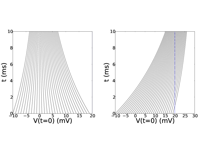
Under the usual assumptions that guarantee the existence and uniqueness of solutions of Eq. 1 on $M$, one can find integral curves $\vec{v}^{\prime}(t,\vec{v_{0}}(t_{0}))$. If $\vec{v_{0}}$ and $t_{0}$ are suitably chosen on $\partial M$, these curves cover the entire manifold $M$ and every point of $M$ is uniquely defined by a coordinate pair $(\vec{v}^{\prime},t)$.

These curves are the characteristics of Eq. 2. Applying the method of characteristics one finds that the total time derivative of the density in the $(\vec{v}^{\prime},t)$ system is given by:

$$\frac{d\rho^{\prime}}{dt}=\int_{M^{\prime}}d\vec{w^{\prime}}\left\{W(\vec{v^{\prime}}\mid\vec{w^{\prime}})\rho^{\prime}(\vec{w^{\prime}})-W(\vec{w^{\prime}}\mid\vec{v^{\prime}})\rho^{\prime}(\vec{v^{\prime}})\right\}$$ (3)

where $\rho^{\prime}(\vec{v}^{\prime},t)=e^{\int^{t}\frac{\partial F(\vec{v}^{\prime})}{\tau\partial\vec{v}^{\prime}}dt^{\prime}}\rho(\vec{v}^{\prime},t)$.

For simplicity, the remainder of the paper will consider one dimensional neuronal models subject to external Poisson distributed spike trains, each spike causing an instantaneous jump in the membrane potential (the case of more than one input, or step sizes $h$ that originate from a distribution of synaptic efficacies can be handled easily):

$$W(v^{\prime}\mid v)=\nu\delta(v^{\prime}-h-v),$$ (4)

leading to:

$$\frac{d\rho}{dt}=\nu\left\{\rho(v^{\prime}-v^{\prime}_{h},t)-\rho(v^{\prime},t)\right\}+r(t)\delta(v^{\prime}-v^{\prime}_{reset}),$$ (5)

Here $r(t)=\int^{v^{\prime}_{th}}_{v^{\prime}_{th,h}}\rho(w,t)dw$; the $\delta$ peak reflects the reset of neurons that spiked to their reset potential.

Equation 5 is the Master equation of an inhomogeneous Poisson process. When considered over a sufficiently short time scale, the solution of this process can be approximated by a homogeneous one, for which efficient numerical and analytic methods are available [28]. The main technical problem associated with solving Eq. 5 is to find a grid that adequately represents the density, not only at $t=0$, but also at later times. Note that in $v^{\prime}$-space all evolution is due to synaptic input, as in the absence of noise $\frac{d\rho(v^{\prime},t)}{dt}=0$.

This idea works well for leaky-integrate-and-fire neurons [27]:

$$\tau\frac{dV}{dt}=-V+I,$$ (6)

where $V$ is the membrane potential and $I$ an external (non-stochastic) current. Here $v^{\prime}$-space slowly expands, which can be accommodated for by adding points to the grid representing the density profile during simulation. Occasionally one must rebin to curb the resulting growth of the grid (see [27] for details).

Figure 2: Characteristics for the values of $I$: $I=-10$ (top), $I=0$ (middle) and $I=10$ (bottom), on an interval $D=[-10,10]$.

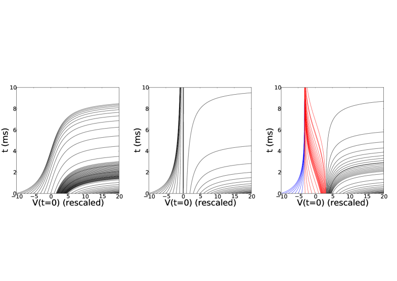
In general neuronal dynamics is not slow compared to synaptic input, e.g. consider the quadratic-integrate-and-fire model given by:

$$\tau\frac{dV}{dt}=V^{2}+I,$$ (7)

where $V$ is a rescaled dimensionless variable. The characteristics can be calculated analytically (Table 1), and are shown in Fig. 2. Their topology depends on the value of $I$. It is clear that some curves run away to infinity in finite time: these neurons are intrinsically spiking. Upon reaching infinity, or some threshold potential $V_{th}$, these neurons are reintroduced in the system at $V=V_{reset}$.

$I>0$	$t=\frac{\tau}{\sqrt{I}}\left\{\arctan\frac{V}{\sqrt{I}}-\arctan\frac{V_{0}}{\sqrt{I}}\right\}$	$V(t)=\sqrt{I}\tan\left\{\sqrt{I}\frac{t}{\tau}+\arctan(\frac{V_{0}}{\sqrt{I}})\right\}$
$I=0$	$t=\frac{\tau}{V_{0}}-\frac{1}{V}$	$V(t)=\frac{V_{0}}{1-V_{0}\frac{t}{\tau}}$
$I<0$	$t=\frac{\tau}{2\sqrt{I}}\ln\left\{(\frac{V-\sqrt{I}}{V+\sqrt{I}})(\frac{V_{0}+\sqrt{I}}{V_{0}-\sqrt{I}})\right\}$	$V(t)=\sqrt{I}\frac{(\sqrt{I}+V_{0})e^{-2\sqrt{I}\frac{t}{\tau}}-(\sqrt{I}-V_{0})}{(\sqrt{I}+V_{0})e^{-2\sqrt{I}\frac{t}{\tau}}+(\sqrt{I}-V_{0})}$

Table 1: QIF Characteristics

The solutions to Eq. 1, for different values of $I$.

At first sight, it seems hard to find an adequate density representation without being forced to rapid and expensive rebinning operations that must be applied in brief succession. However, by adopting a grid whose bin limits are defined by the characteristics rebinning operations can be avoided altogether. Fast dynamics will result in large bins, slow dynamics in small ones. Large bins, however, do not introduce inaccuracy, because all density within the same bin will share a common fate. This is true even after reset. This observation is crucial and applies quite generally. For this reason we will explain it in some detail in the next section.

Representing fast dynamics

Figure 3: Modelling advection requires only a pointer update. Top: At time $t$ each probability bin is associated with a density interval. Bottom: Update at $t+1$.

Starting with a model of the form of Eq. 1, we assume that $\frac{dV}{dt}>0$ everywhere on $(V_{min},V_{th})$, considering more general cases later on.

Consider now the initial value problem, posed by Equation 1 with boundary condition $V(t=0)=V_{0}$. Assuming $V_{0}=V_{min}$, the neuron will reach threshold $V_{th}$ in finite time $t_{period}$. The neuron will then be reintroduced at $V_{reset}$. For simplicity $V_{reset}=V_{min}$ will be assumed, for a practical implementation of the algorithm this is immaterial. Consider now a division of time interval $t_{period}$ into $N$ time steps:

$$t_{step}\equiv\frac{t_{period}}{N}$$ (8)

The density profile $\rho(v)$ for given time $t$ will be represented in a grid consisting of $N$ bins. We define the bin limits as follows: each bin $i$ ($i=0,\cdots,N-1$) corresponds to a potential interval $[v_{i},v_{i+1})$ in the following way: $v_{0}=V_{min}$, and when $V(t=0)=V_{min}$, $v_{i}$ is given by:

$$v_{i}\equiv V(it_{step}),i=0,\cdots,N,$$ (9)

where $V(t)$ is the solution of Eq. 1. Note that there are $N+1$ bin limits and that by definition $V_{N}\equiv V_{th}$. In general, the binning is non-equidistant. When a neuron spikes, for example, it traverses a considerable potential difference in a short period of time and the bins covering this traversal will be very large. The evolution of a population density profile defined on $(V_{min},V_{th})$ can now be modeled as follows. A probability grid $\mathcal{P}$ is created of size $N$. An array $\mathcal{V}$ contains the bin limits of $\mathcal{P}$. We define element $i$ of $\mathcal{V}$, $\mathcal{V}_{i}\equiv v_{i}$. Assume an initial density profile $\rho(v,0)$ is defined at $t=0$. We represent this profile by setting $P_{i}$ to:

$$P_{i}\equiv\rho(v_{i},0)(v_{i+1}-v_{i}),$$ (10)

so that $P_{i}$ approximates the total probability between $V=v_{i}$ and $V=v_{i+1}$. Remarkably, having defined the contents of $\mathcal{V}$ and $\mathcal{P}$, they can remain constant, yet describe advection: the evolution of the density in the absence of synaptic input. To see this, consider the evolution over a period of time $t_{step}$. All neurons that previously had a potential between $V=v_{i}$ and $V=v_{i+1}$, will now have a potential between $V=v_{i+1}$ and $V=v_{i+2}$, except for those that had a potential between $V=v_{N-1}$ and $V_{th}$ who now have a potential between $V=V_{min}$ and $V=v_{1}$. So, the relationship between $\mathcal{V}$ and $\mathcal{P}$ changes, but not the actual array contents themselves. Specifically, the density profile at simulation time $t_{sim}=jt_{step}$ is given by:

$$\rho(v_{i},t_{sim})=\frac{P_{(i-j)\bmod N}}{v_{i+1}-v_{i}}$$ (11)

This is all that is required to represent the density profile in $v^{\prime}$-space; the computational overhead is negligible as an implementation of this idea only requires a pointer update without any need for shuffling data around (see Fig. 3).

Equation 5 can be solved by assuming that during $t_{step}$ neurons only leave their bin due synaptic input. It is also assumed that, although the magnitude of $h$ is dependent on $v^{\prime}$, it is constant during the small time $t_{step}$. The solution method is not really different from that described in [29, 27, 28], but is complicated by the non-equidistance of the probability grid $\mathcal{P}$. Where in the original implementation only the magnitude of the synaptic efficacy had to be recalculated in $v^{\prime}$-space to find the transition matrix of the Poisson process, here a search is needed to locate the density bin that will receive probability from a given density bin, as the jump size $h^{\prime}$ becomes dependent on $v^{\prime}$ in $v^{\prime}$-space. This issue is rather technical and is be explained in detail in “Methods: Synaptic Input: Solving the Master Equation”.

Figure 4: Density profile of QIF population decorrelated by large synapses. Line: population density; markers: Monte Carlo simulation.

Switching Topologies: Current Compensation

The idea is most easily illustrated for a Poisson process. In one dimension, for a single synaptic input with postsynaptic efficacy $h$ receiving a single Poisson distributed input rate $\nu$, the population density equation is given by [8]:

$$\frac{\partial\rho}{\partial t}+\frac{\partial}{\partial v}(\frac{F(v)\rho(v)}{\tau})=\nu\left\{\rho(v-h)-\rho(v)\right\}$$ (12)

Consider the limit $h\rightarrow 0$, such that $\nu h=\mbox{constant}$. A Taylor expansion of the right hand side up to order $h^{2}$ then gives:

$$\frac{\partial\rho}{\partial t}+\frac{\partial}{\partial v}\left\{\frac{F(v)\rho}{\tau}+\rho h\nu-\frac{\nu h^{2}}{2}\frac{\partial\rho}{\partial v}\right\}=0$$ (13)

Now define:

$$\mu \equiv\nu h\tau$$

$$\sigma^{2} \equiv\nu h^{2}\tau$$ (14)

and Eq. 13 becomes a Fokker-Planck equation:

$$\frac{\partial\rho}{\partial t}+\frac{\partial}{\partial v}\left\{\rho\frac{F(v)+\mu}{\tau}-\frac{\sigma^{2}}{2\tau}\frac{\partial\rho}{\partial v}\right\}=0$$ (15)

This equation describes the evolution of the density due to the deterministic dynamics, determined by $F(v)$ and an additive Gaussian white noise with parameters $\mu$ and $\sigma$.

It is clear that Eq. 15 is invariant under the transformation:

$$\left\{\begin{array}[]{rl}F(v)&\rightarrow F(v)+I_{c}\\ \mu&\rightarrow\mu-I_{c}\end{array}\right.$$ (16)

for any constant current value $I_{c}$, i.e. one add a DC component to a neuron when a similar mean contribution is subtracted from its input. This result is valid beyond the diffusion approximation, as it still holds when higher than second order derivatives are considered in the procedure used to derive Eq. 15.

Table 2: Default simulation parameters for QIF neurons.

$N$	300
$\tau$	$10^{-2}$ s
$\tau_{ref}$	0 s
$V_{min}$	-10
$V_{max}$	10
$V_{reset}$	-10
$I_{c}$	0.2
$\sigma_{c}$	0.01
$h_{diff}$	0.03

Examples

We will give a number of examples. For quadratic-integrate-and-fire neurons the default simulation parameters are given Tab. 2. In the remainder only deviations will be listed.

Example 1: quadratic-integrate-and-fire neurons with extremely large synapses
Figure 4 demonstrates the validity of the method beyond the diffusion limit. A periodically firing group of neurons, firing in synchrony at the start of the simulation, is decorrelated by a low frequency (5 Hz) high impact ($h=5$, this is half of the entire interval!) input. The density profile is a slowly collapsing delta-peak, travelling along the characteristics of a periodically firing quadratic-integrate-and-fire neuron for several seconds, before reaching its steady state profile. We show the density profile in Fig. 4 at $t=0.02,0.12$ and $9.9$ s.

At no moment the population density is well described by a diffusion process, and the steady state firing rate deviates considerably from that predicted by numerical calculations based on the diffusion approximation. At $t=0.12$ s, the density profile shows a fine structure that is indeed borne out by large-scale Monte Carlo simulations. We are not aware of a method sensitive to the density gradient that could have modeled this accurately.

Figure 5: Examples of the evolution of the density of a population of QIF neurons under the influence of Gaussian white noise input.

Example 2: quadratic-integrate-and-fire neurons in the diffusion limit
A single Poisson input, or a combination of one excitatory and one inhibitory Poisson input, can emulate a Gaussian white noise (see “Methods: Emulation of Gaussian white noise”). We will study both the density transient density profiles and the resulting firing rate response of the population (a neuron reaching threshold will emit a spike and reset to reset potential. The population firing rate is fraction of neurons that in a time interval, divided by that time interval).

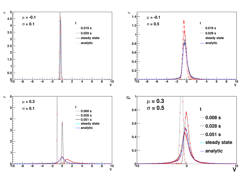
In Fig. 5 the transient density profiles are shown for four different $(\mu,\sigma)$ combinations. The negative input, small noise distribution ($\mu=-0.1,\sigma=0.1$) peaks at the stable equilibrium point. Almost no neurons are pushed across the second, instable equilibrium point and this population does not fire in response to its input (see Fig. 7). For higher noise values, the peak is smeared and some neurons are pushed across the unstable, leading to an appreciable firing rate; a deterministic current with similar mean would evoke no response (see Fig. 7).

Figure 6: Steady state density profiles in response to Gaussian white noise.

Figure 7: Transient firing rates inresponse to Gaussian white noise.

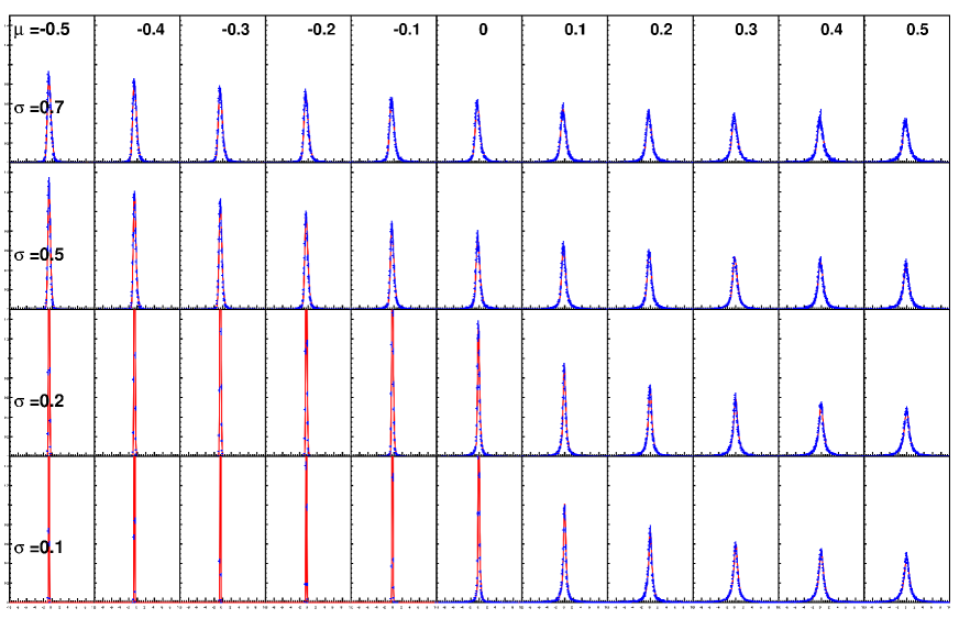
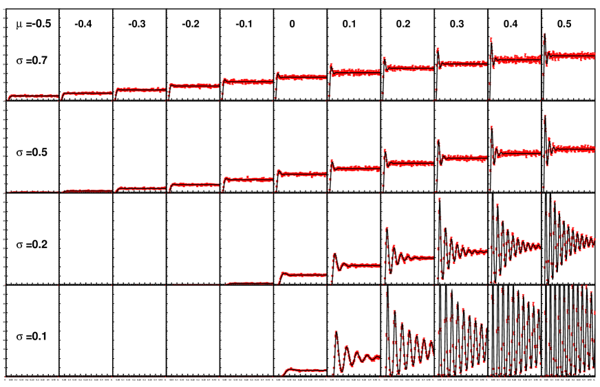
A larger mean $\mu=0.3$ evokes a clear response, and the peak of the density is clearly driven across $V=0$. Unlike in Example 1, this peak will soon collapse. It will approach its steady state distribution but demonstrate small oscillations that are clearly visible in the firing rate for a long time. At higher noise, the steady state is reached faster and the firing rates transients die out much faster (Fig. 7).

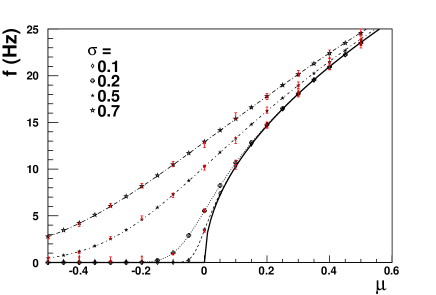
Figures 6 and 7 provide a summary of the diffusion results for $\mu\in[-0.5,0.5]$ and $\sigma=0.1,0.2,0.5,0.7$. Figure 7 shows the transient firing rates are shown and compared to Monte Carlo simulations (red markers). Figure 6 shows the density profiles for large time $t=9.9$ s, when profiles should assume their steady state (grey line, but barely visible since Monte Carlo and analytic results agree and are overlaid). Markers show Monte Carlo results, red lines are calculated directly from the diffusion approximation, using the integration scheme from [15]. Figure 8 shows the so-called gain curves, the steady state firing rates that can be read of Fig. 7 in black markers. Monte Carlo results are indicated by red markers, lines are calculated analytically from the diffusion approximation [30]. All results are in excellent agreement with each other.

Figure 8: Gain curves. Lines: analytic steady state firing rates. Red error bars: Monte Carlo simulation, black markers: population density results.

Example 3: The gain curve is changed by large synapses.
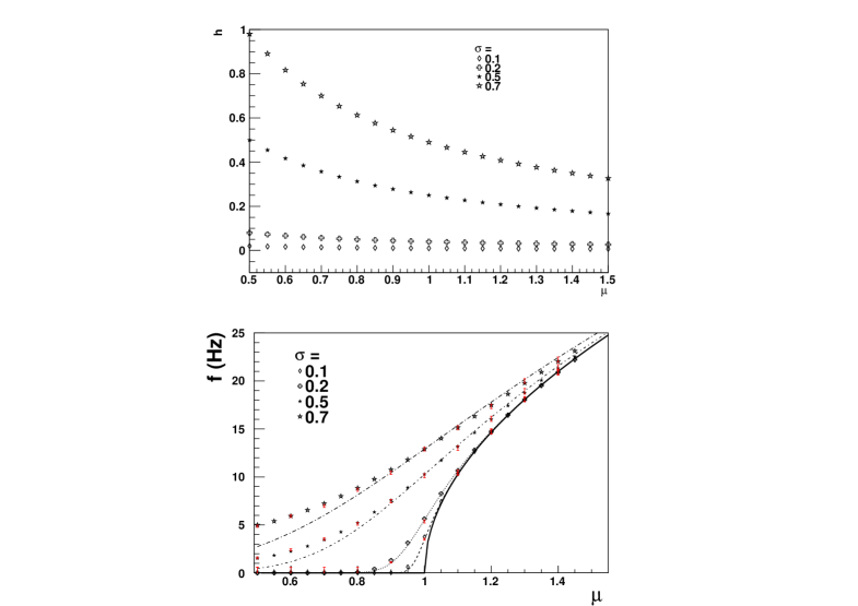
A single Poisson input can only approximate Gaussian white noise as long as the variability is much smaller than the mean of the signal. Figure 9 (top) shows the efficacy $h$ as a function of $\mu$ for different $\sigma$ values, and hence indicate where deviations can be expected (namely for large $h$).

Figure 9 shows a population receiving input from a single Poisson input with firing rate and efficacy calculated using Eq. 30. $\mu$ must not be interpreted as the DC contribution of a Gaussian white noise input.

A value of $I=-1(I_{c}=1.1)$ was chosen and simulated both in Monte Carlo and using the population density approach. Here, one expects the population to fire when the neurons’ negative $I$ value is overcome, i.e. for $\mu>1$.

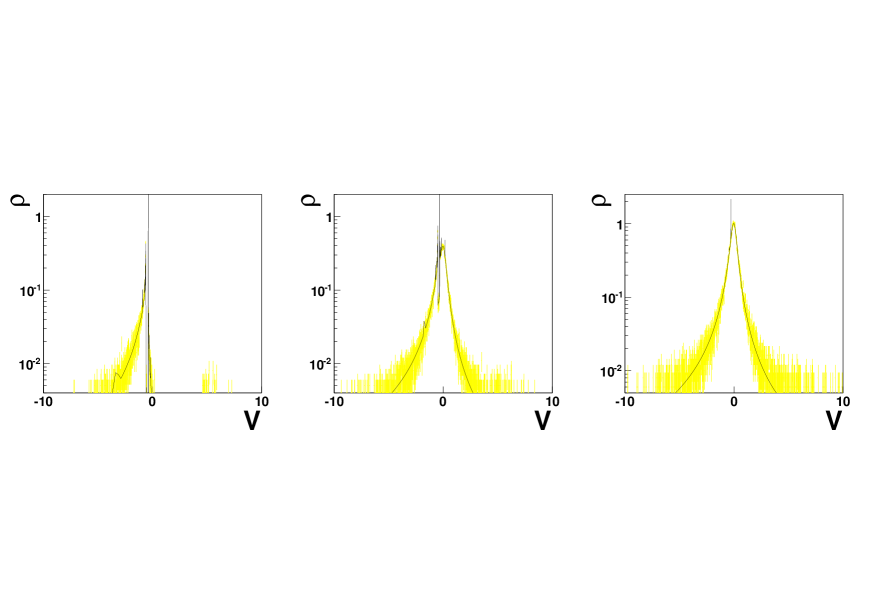
The steady state values of the population density approach are in excellent agreement with the Monte Carlo, but both deviate from the gain curves that are calculated in the diffusion approximation (Fig. 9 (bottom)), precisely where this would have been expected according to Fig. 9 (top). Note, however, that for the first time it was necessary to smear the synaptic efficacies slightly ($\sigma=0.01$). In the absence of smearing, there would have been a disagreement between Monte Carlo and data for low $\sigma$. This is due to the fact that the variability of the compensation current $I_{c}$ cannot be chosen arbitrarily low as this would entail artificially high firing rates that would render the solution of the Master equation inefficient. A reasonable minimum value is $\sigma=0.01$.

As can be seen from Fig. 9, the jumps are really large for $\sigma=0.7$ and low $\mu$. Indeed, there the deviation from the diffusion approximation is substantial, but there is no visible disagreement between Monte Carlo and population density approach. This is all the more impressive because to model negative $I$ values, current compensation with $I_{c}=1.1$ had to be used, and demonstrates the viability of the current compensation approach.

When the steady state density profile obtained with the population density method is compared to that obtained from the Monte Carlo, again good agreement is found, while a small but significant deviation from the density profile calculated from the steady state, of the Fokker-Planck equation Eq. 15 can be seen for large $\sigma$ and low $\mu$ (Fig. 9 (top)).

Figure 9: For large synapses the gain curve changes. Top: Jump size for a single Poisson input emulating Gaussian white noise. Bottom: Monte Carlo (red markers), population density results (black markers) and diffusion prediction (lines).

Example 4: Universality: quadratic- and leaky-integrate-and-fire neurons are handled by the same algorithm.
We use current compensation to turn leaky-integrate-and-fire neurons into spiking neurons. We add a small constant current $I_{c}=1.1$ as in Eq. 6. Without this current the characteristics move away from threshold, with this current they cross threshold (compare Fig. 1 left and right).

A Gaussian white noise current emulated by Poisson input with mean $\mu=-1.1$ and small variability ($\sigma=0.05$) is presented as input. This is combined with a single Poisson input of 800 Hz with synaptic efficacy $h=0.03$. This example was used in earlier studies as a benchmark [8, 27]. In Fig. 10 the steady state density profile and the firing rate of the population are shown. They are compared to the simulation without current compensation, described earlier [27], using a density representation tailored to leaky-integrate-and-fire characteristics (red line).

Figure 10: Algorithm works for both QIF and LIF neurons. Top: steady state density profile for current compensation (black), dedicated LIF neuron implementation (red). Bottom: output firing rates.

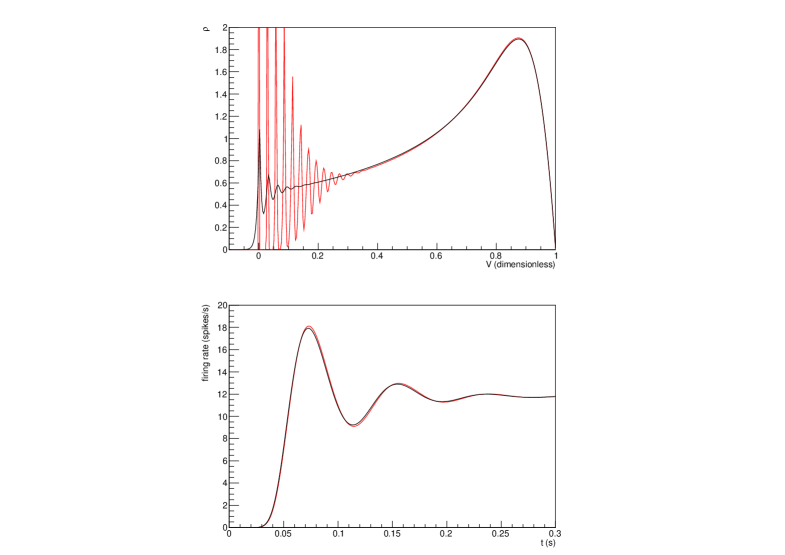
The results are almost identical. In the original simulation the steep peaks are the consequence of a single synaptic efficacy. Sirovich [29] has shown analytically that for the first peak the density profile is discontinuous, for the second peak the first derivative is discontinuous, and so on. This is not necessarily realistic in terms of neuroscience, but it demonstrates once more that the method can handle the jagged density profiles that result from finite size jump processes.

In the current compensation version of the simulation, the small variability of the compensation current smears these peaks. The noise also slightly reduce the extremes of the firing rate (Fig. 10), but otherwise the agreement is excellent. The effect of the smearing due to the compensation current is equivalent to effects caused by spread in the synaptic efficacies [30]. Moreover, many brain systems receive an unspecific background that must be modeled as noise anyway, so current compensation can be applied quite generally in neuroscience.

Importantly, the only change that had to made to change over from quadratic- to leaky-integrate-and-fire neurons is in the calculation of array $\mathcal{V}$, which is done during the initialization of the algorithm.

Figure 11: High level overview of the approach. Neural model (red) only enters explicitly is in $\mathcal{V}$.

Discussion

We presented a method for numerically solving the differential Chapman-Kolmogorov equation for large jumps. We demonstrated the validity of the approach by comparing population density results for neuronal populations receiving input from large synapses to Monte Carlo simulations, and neurons receiving input from small synapses to analytic or numerical results obtained in a diffusion approach. We presented two examples (Example 1 and 4) that demonstrate that the method can handle arbitrary jump sizes and the extremely jagged density profiles that result.

We also demonstrated that the algorithm is universal: it can handle any one dimensional neural, subject to the condition that a (pseudo) diffusive background of small variability is allowed. This point is obvious mathematically, the transformation from the differential Chapman-Kolmogorov equation to the Master equation of the noise process can always be performed [27]. The challenge is to find a suitable density representation. Periodically spiking neurons yield a particularly simple density representation, and using current compensation a non spiking neural model can be made to spike. In practice the compensation current will always introduce some variability. Where variability is present already, for example because the input is noise or because synaptic efficacies are variable, this extra variability can be absorbed and has no bearing on the simulation results.

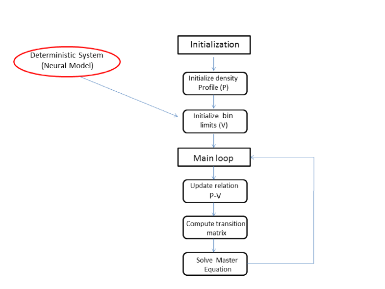
The universality of the algorithm is reflected in the implementation. Although the neuronal model defines the grid boundaries of the density representation - the content of grid $\mathcal{V}$, it does so before simulation starts. This means that neuronal models can be exchanged with great simplicity. To provide a neural model is to provide the contents of grid $\mathcal{V}$. This is the only place were the neuronal model enters the method explicitly. This important point is emphasized in Fig. 11, which provides a high level overview of the method.

We demonstrated the method using a Poisson process and showed that if the jump size becomes small, diffusion results are recovered. The use of Poisson statistics is appropriate in neural simulations. An individual neuron will receive at most of the order of $10^{5}$ spikes per seconds. At such rates, a Poisson Master equation can solved efficiently. We found that 1 simulation second could be handled in between a 0.5 and 2.0 s real time, which is an order of magnitude faster than Monte Carlo - based on comparisons to leaky-integrate-and-fire simulations in NEST [31] where a 10000 neuron population achieves real time ratios of approximately 30. We found an excellent recovery of diffusion results whenever the jump size is 5 % of the interval for low noise and of the order of 10 % for high noise conditions (Fig. 9).

It is conceivable that in other applications jump sizes are smaller. Artificially small jump sizes would lead to very high firing rates for a Poisson master equation. We find that adopting a jump size of less than 1 % of the interval leads to inconveniently high firing rates. The method is clearly best used for finite jump sizes.

To study diffusion, it would be interesting to consider a finite difference scheme for solving Eq. 15 with $F(v)=0$. This would allow a direct comparison to diffusion results, while still benefitting from the universality of this approach. For example, it would still be possible to compare diffusion in different neural models without the need to derive a separate Fokker-Planck equation for each case. Cox and Ross [32] have shown that explicit finite difference schemes for solving equations of the type 15 correspond to a jump process with three possibilities: a move left, right or no move in the grid. Brennan and Schwartz [25] have shown that implicit finite difference scheme corresponds to a jump process where jumps to every other position are allowed. For suitable parameters and in the limit of an infinitely fine grid both schemes converge to a diffusion process, where the implicit scheme is unconditionally stable. These results are interesting because they suggest suitable Master equations to arrive at good diffusion approximations. In the context of neural systems this discussion is to some extent academic as true diffusion conditions are not realized in the brain, but most analytic results on population densities have been derived in the diffusion approximation, and a comparison is valuable.

The ideas presented here constitute an approach rather than an algorithm. There is an endless variation of noise processes and dynamical systems that can be combined. Colored noise can be handled by a two-step approach: the Master equation of a colored noise process can be simulated by leaky-integrate-and-fire population receiving white noise.

The technique was demonstrated on one dimensional neural populations. Such models are simple enough to demonstrate the applicability of the technique to a wider audience. Whether it can be successfully employed to more complex neural models is an open question. Fortunately, there is a tendency to move from complex conductance-based models to simpler low dimensional effective model neurons, see e.g. [33]. The population density approach still is competitive in two dimensions [14].

We hope that the technique will find widespread application. Depending on the application area, the methods described here may need adaptation. The current compensation technique may not work for all applications as the extra variability introduced by the compensation current might not always be acceptable. However, this is no fundamental objection to using this approach. Applying a combination of techniques described here and earlier [27, 28] useful density representations may still be found, although their implementation may be limited to a specific topology of the deterministic flow.

Methods

Solutions in absence of synaptic input

Consider a neuron in the absence of synaptic input, but receiving a constant input current $I$. In general Equation 1 can be used to evolve the state of a neuron that has potential $V_{0}$ at $t=0$. For some cases analytic solutions exist. For leaky-integrate-and-fire neurons:

$$V(t)=I-(I-V_{0})e^{-\frac{t}{\tau}}$$ (17)

For quadratic-integrate-and-fire neurons, the solutions of Eq. 7 depend on the sign of $I$, and there are clear topological differences between solutions for different $I$. They are given in Tab. 1 and shown in Fig. 2.

Derivation of the population density equation

The population density approach can be motivated as follows and is not restricted to one dimensional neuronal models. To reflect that, this section will consider the more general model:

$$\tau\frac{d\vec{v}}{dt}=\vec{F}(\vec{v})$$ (18)

Assume that $\mathcal{M}$ is an open subset of $\mathbb{R}^{n}$, where $n$ is the dimensionality of the neuronal point model defined by Eq. 18. Assume that the neuronal state is given by point $\vec{v}$ in $\mathcal{M}$. Further, assume that a density function $\rho(\vec{v},t)$ is defined on $\mathcal{M}$ and that $\rho(\vec{v},t)d\vec{v}$ represents the probability for a given neuron to be in the state space element $d\vec{v}$ at time $t$. Consider the evolution of neuronal states for neurons in $d\vec{v}$ during a short period of time $dt$. If external input is ignored, then under the influence of neuronal dynamics all neurons, and no others, that were in $d\vec{v}$ at time $t$ are in volume element $d\vec{v}^{\prime}$ at time $t^{\prime}$, with $\vec{v}^{\prime}$ and $t^{\prime}$ defined by:

$$\left\{\begin{array}[]{rl}t\rightarrow&t^{\prime}=t+dt\\ \vec{v}\rightarrow&\vec{v}^{\prime}=\vec{v}+\vec{dv}=\vec{v}+\frac{\vec{F}}{\tau}dt\end{array}\right.$$ (19)

Conservation of probability requires:

$$\rho(\vec{v},t)d\vec{v}=\rho(\vec{v}^{\prime},t^{\prime})d\vec{v}^{\prime}.$$ (20)

Using:

$$\rho(\vec{v}^{\prime},t^{\prime})=\rho(\vec{v},t)+dt\frac{\partial\rho(\vec{v},t)}{\partial t}+d\vec{v}\cdot\frac{\partial\rho(\vec{v},t)}{\partial\vec{v}},$$ (21)

Equation 20 becomes:

$$\left\{\rho(\vec{v},t)+d\vec{v}\cdot\frac{\partial\rho(\vec{v},t)}{\partial\vec{v}}+dt\frac{\partial\rho(\vec{v},t)}{\partial t}\right\}d\vec{v}^{\prime}=\rho(\vec{v},t)d\vec{v}$$ (22)

Since

$$d\vec{v}^{\prime}=\mid J\mid d\vec{\vec{v}},$$ (23)

with:

$$\mid J\mid=\mid\frac{\partial\vec{v}^{\prime}}{\partial\vec{v}}\mid=\mid\mathbb{I}+\frac{1}{\tau}\frac{\partial\vec{F}(\vec{v})}{\partial\vec{v}}dt\mid+O(dt^{2}),$$ (24)

so that, collecting all terms up to $O(dt)$:

$$\left\{\frac{1}{\tau}\frac{\partial\vec{F}(\vec{v})}{\partial\vec{v}}\rho+\frac{\partial\rho}{\partial t}+\frac{\vec{F}(\vec{v})}{\tau}\cdot\frac{\partial\rho}{\partial\vec{v}}\right\}d\vec{v}=0.$$ (25)

Since this equation must hold for infinitesimal but arbitrary volumes $d\vec{v}$, it follows that:

$$\frac{\partial\rho}{\partial t}+\frac{1}{\tau}\frac{\partial}{\partial\vec{v}}\cdot(\vec{F}\rho)=0$$ (26)

Equation 26 is an advection equation for probability flow under the influence of neuronal dynamics. When noise is also considered the equation becomes:

$$\frac{\partial\rho}{\partial t}+\frac{1}{\tau}\frac{\partial}{\partial\vec{v}}\cdot(\vec{F}\rho)=\int_{M}d\vec{w}\left\{W(\vec{v}\mid\vec{w})\rho(\vec{w})-W(\vec{w}\mid\vec{v})\rho(\vec{v})\right\}.$$ (27)

This is an example of what Gardiner calls the differential Chapman-Kolmogorov equation [24]. In the remainder only Poisson processes will be considered, but the method is applicable to any noise process that can be modeled by a Master equation. For a single Poisson input $W(\vec{v}^{\prime}\mid\vec{v})$ is given by:

$$W(\vec{v^{\prime}}\mid\vec{v})=\nu\delta(v^{\prime}_{0}-v_{0}-h)$$ (28)

Here $\nu$ is the rate of the Poisson process, it is assumed that one of the neuronal state variables, $v_{0}$ instantaneously transitions from $v_{0}$ to $v_{0}+h$, where $h$ is the synaptic efficacy. In a one dimensional neuronal model $v_{0}$ is $V$, the membrane potential. Clearly, not all synapses in a population have a single value, and often one assumes:

$$W(\vec{v^{\prime}}\mid\vec{v})=\nu\int dhp(h)\delta(v^{\prime}_{0}-v_{0}-h),$$ (29)

where $p(h)$ is often assumed to be Gaussian [8, 30]. In a network where many populations connect to any given population, multiple contributions of the form Eq. 29 must be included - one for each separate input. In principle, each input must be modeled separately, but often many inputs can be subsumed into a single one using the central limit theorem, leading to a Gaussian white noise input contribution. Sometimes kernels $p(h)$ of separate inputs overlap and can be integrated into one input contribution.

Figure 12: Emulation of a Gaussian white noise with Poisson inputs. Left: isoline of $h=0.01V_{th},h=0.1V_{th}$. Right: synaptic efficacies are fixed at 3 % of $V_{th}$. Blue (red) lines are isolines of frequency of excitatory (inhibitory) inputs.

Figure 13: The Master equation follows from translating the contents of grid $\mathcal{V}$ the synaptic efficacy.

Emulation of Gaussian white noise and the breakdown of the diffusion approximation

It is evident that by choosing a small efficacy $h$ and large input rate $\nu$, the Poisson input approximates additive Gaussian white noise. These parameters must be chosen such that they provide the correct $\mu$ and $\sigma$. Inverting Eq. 14 gives:

$$h =\frac{\sigma^{2}}{\mu}$$

$$\nu =\frac{\mu^{2}}{\tau\sigma^{2}}$$ (30)

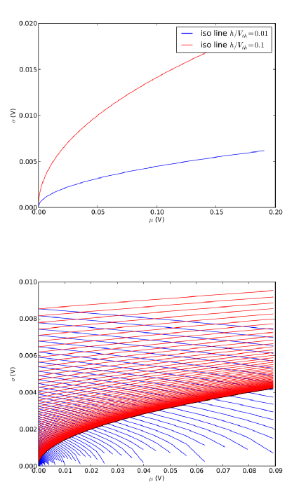
A single Poisson input can only emulate a Gaussian white noise when $h$ is small compared to the relevant potential difference, e.g. for leaky-integrate-and-fire neurons when $\mid h\mid\ll V_{th}$, or $\mid h\mid\ll I$ for quadratic-integrate-and-fire neurons, i.e. not for all values of ($\mu$,$\sigma$) can values for $h$ and $\nu$ be found so that the diffusion regime is reliably reproduced. This is borne out by Fig. 12 (left). Here a neuron is considered with $\tau=10$ ms, $V_{th}(\equiv\theta)=20$ mV. For a $(\mu,\sigma)$ plane isolines of $h$ are plotted: one where $h$ is precisely at 1% of the threshold potential, one where it is at 10%.

It is clear that a single Poisson input can emulate a broad range of $\mu$ values, but only at low $\sigma$. Using two inputs, one excitatory and one inhibitory, one can fix the synaptic efficacies at a low value compared to $V_{th}$. If this value is $J$ one finds:

$$\mu =\tau J\nu(\nu_{e}-\nu_{i})$$

$$\sigma^{2} =\tau\nu J^{2}(\nu_{e}+\nu_{i})$$ (31)

One then has two frequencies $\nu_{e}$ and $\nu_{i}$ as free parameters. This setup covers most of the $(\mu,\sigma)$ plane, except for values at low $\sigma$, where the input frequency of the inhibitory input falls below 0. In Fig. 12 only frequency isolines for positive input frequencies are shown. The boundary where the inhibitory input rate falls below 0 is forbidden for two inputs, but this is precisely the area covered by a single input (clearly if $\nu_{i}=0$, we have a single excitatory input). The arguments presented here cover a positive range of $\mu$, similar arguments can be made for a net inhibitory input.

In summary, one needs either one or two Poisson inputs to emulate a Gaussian white noise. In particular, this implies that we can use a single excitatory input as a model for the gradual breakdown of the diffusion limit: if we increase $\sigma$ and calculate the synaptic efficacy using Eq. 30, we should see deviations from the diffusion limit as $h$ can no longer be considered to be small.

This is shown in Fig. 9 which shows the step size for a single Poisson input given $\mu$, $\sigma$. For $\sigma$ comparable to $\mu$ this step size is not necessarily small compared to the potential scale on which the neuronal model is defined and deviations of the diffusion approximation can be expected.

Whenever a Gaussian white noise with very small variability is required, this must be delivered by a single Poisson input. The firing rate is then inversely proportional to the jump size. For very low variability a numerical solution of the Poisson process may become inefficient.

Synaptic input: solving the master equation

Now consider a single Poisson input. The evolution of the density profile is straightforward in principle but complicated by the bins being non-equidistant. Formally the noise process can be represented as a transition matrix. Figure 13 how this matrix can be determined: the contents of grid $\mathcal{V}$ are shifted by an amount $h$, where $h$ is the synaptic efficacy. Probability moves from potential $V-h$ to $V$ as consequence of an input spike. In large bins this means that neurons stay mostly within the same bin. Neurons that are in small bins may end up several bins higher. Below we will examine this process in detail.

Figure 14: Transition matrices for QIF (top) and LIF neurons (bottom). Loss of probability is indicated by black, gain by white.

To determine the Poisson Master equation for excitatory input $(h>0)$, consider that every neuron arriving in the interval $D_{i}=[v_{i},v_{i+1})$ must have come from $D_{i,h}=[\max(v_{i}-h,V_{min}),v_{i+1}-h)$. Consider, the $N+1$ integers defined by:

$$p_{i}\equiv\left\{\begin{tabular}[]{ll}$v_{i}-h<v_{0}$:&-1\\ $v_{i}-h\geq v_{0}$:&$\underset{k}{\operatorname*{arg\,min}}\ v_{k}\leq v_{i}-h<v_{k+1}$\end{tabular}\right.$$ (32)

Now consider $i=0\cdots N-1$; if $p_{i}=p_{i+1}$, $\alpha_{i,p_{i}}$ is given by:

$$\alpha_{i,p_{i}}\equiv\frac{v_{i+1}-v_{i}}{v_{p_{i}+1}-v_{p_{i}}};$$ (33)

For $p_{i}=-1$, $\alpha_{i,l}=0$. If $p_{i}<p_{i+1}$, $\alpha_{i,l}$ is given by:

$$\alpha_{il}\equiv\left\{\begin{tabular}[]{rl}$l=p_{i}$:&$\theta_{l}\frac{v_{p_{i}+1}-(v_{i}-h)}{v_{p_{i}+1}-v_{p_{i}}}$\\ $p_{i}<l<p_{i+1}$:&1\\ $l=p_{i+1}$:&$\frac{v_{i+1}-h-v_{p_{i+1}}}{v_{p_{i+1}+1}-v_{p_{i+1}}}$\end{tabular}\right.$$ (34)

with:

$$\theta_{l}\equiv\left\{\begin{tabular}[]{rl}$l<0$:&0\\ $l\geq 0$:&1\end{tabular}\right.$$ (35)

Finally,

$$\beta_{i}\equiv\left\{\begin{tabular}[]{rl}$i<p_{N}$:&0\\ $i=p_{N}$:&$\frac{v_{p_{N}+1}-v_{N}+h}{v_{p_{N}+1}-v_{p_{N}}}$\\ $i>p_{N}$:&1.\end{tabular}\right.$$ (36)

From this the Master equation at $t=kt_{step}$ follows:

$$\frac{dP_{i-k\bmod N}}{dt}= -P_{i-k\bmod N}+\sum^{p_{i+1}}_{l=p_{i}}\alpha_{i,l}P_{l-k\bmod N}$$ (37)

$$+ \delta_{iR}(\sum^{N-1}_{l=0}\beta_{l}P_{l-k\bmod N}),$$ (38)

where $R$ is defined by:

$$R\equiv\underset{k}{\operatorname*{arg\,min}}\ v_{k}\leq V_{reset}\leq v_{k+1}$$ (39)

and $\delta$ is the Kronecker $\delta$. The term including it reflects the re-entry of neurons at the reset potential once they have spiked.

For inhibitory input $(h<0)$, the formulae are almost identical as now $v-h$ refers to a higher potential. Again, define

$$\tilde{p}_{i}\equiv\left\{\begin{tabular}[]{ll}$v_{i}-h>v_{N}$:&$N$\\ $v_{i}-h\leq v_{N}$:&$\underset{k}{\operatorname*{arg\,min}}\ v_{k}\leq v_{i}-h<v_{k+1}$\end{tabular}\right.$$ (40)

Again consider $i=0\cdots N-1$; if $\tilde{p_{i}}=\tilde{p}_{i+1}$, $\tilde{\alpha}_{i,\tilde{p}_{i}}$ is given by:

$$\tilde{\alpha}_{i,p_{i}}\equiv\frac{v_{i+1}-v_{i}}{v_{\tilde{p}_{i}+1}-v_{\tilde{p}_{i}}};$$ (41)

if $p_{i}<p_{i+1}$, $\tilde{\alpha}_{i,l}$ is given by:

$$\tilde{\alpha}_{il}\equiv\left\{\begin{tabular}[]{rl}$l=\tilde{p}_{i}$:&$\frac{v_{\tilde{p}_{i}+1}-(v_{i}+h)}{v_{\tilde{p}_{i}+1}-v_{\tilde{p}_{i}}}$\\ $\tilde{p}_{i}<l<\tilde{p}_{i+1}$:&1\\ $l=\tilde{p}_{i+1}$:&$\theta_{N-1-\tilde{p}_{i}+1}\frac{v_{i+1}+h-v_{\tilde{p}_{i+1}}}{v_{\tilde{p}_{i+1}+1}-v_{\tilde{p}_{i+1}}}$\end{tabular}\right.$$ (42)

Finally, $\gamma_{i}$ is defined as follows:

$$\gamma_{i}\equiv\left\{\begin{tabular}[]{rl}$i<p_{0}$:&1\\ $i=p_{0}$:&$\frac{v_{p_{0}+1}-(v_{0}+h)}{v_{p_{0}+1}-v_{p_{0}}}$\\ $i>p_{0}$:&0\end{tabular}\right.$$ (43)

The Master equation for an inhibitory input is:

$$\frac{dP_{i-k\bmod N}}{dt}=-(1-\gamma_{i})P_{i-k\bmod N}+\sum^{\tilde{p}_{i+1}}_{l=\tilde{p}_{i}}\tilde{\alpha}_{i,l}P_{l-k\bmod N}$$ (44)

Note that Eqs. 38 and 44 are of the form:

$$\frac{d\vec{P}}{dt}=\mathcal{M}^{(k)}\vec{P},$$ (45)

where $\mathcal{M}^{(e)}$ is the transition matrix resulting from adding individual input contributions of the form 38 and 44.

Solving the master equation

Equation 38 and 44 were solved numerically using Runge-Kutta-Fehlberg integration. This is not optimal, but is very straightforward to implement, and yields a performance that is faster than Monte Carlo simulation by at least one order of magnitude. Note that in Eq. 38 one simply ignores the zero elements of $\mathcal{M}^{(e)}$. The calculation of the time derivatives then scales as $O(N)O(N_{input})$, where $N_{input}$ is the number of inputs that need to considered. In many neural systems, such as cortex it can be assumed that most inputs deliver a background that can be treated as a single noisy input [14, 30]

Different neuronal models: different transition matrices

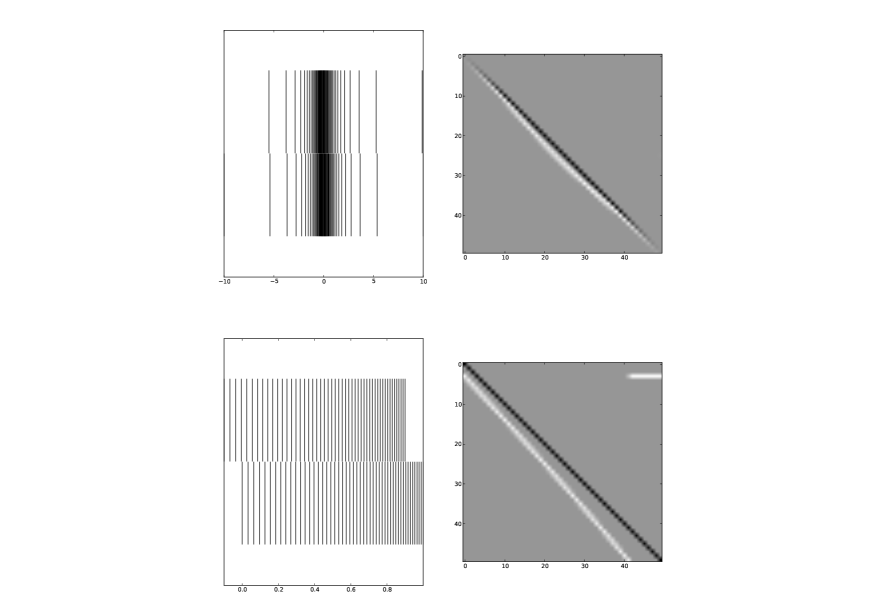
Although the noise process and the neuronal dynamics are independent, the neuronal dynamics determines the representation of the density profile. The bin boundaries of the density profile in $v$-space, $\mathcal{V}$ are given by the evolution of the neuronal state, and therefore the transition matrix is directly dependent on the neuronal model. This is illustrated in Fig. 14, which shows the transition matrix for identical $h,\nu$ for quadratic-integrate-and-fire and leaky-integrate-and-fire neurons. First, it should be observed that to accommodate for spiking behaviour, the state space of the quadratic-integrate-and-fire neuron is much larger, for the leaky-integrate-and-fire neuron it is limited by the threshold, $V_{th}$. Second, the quadratic-integrate-and-fire neuron is a truly spiking model: once it spikes, its state runs away to infinity in finite time. The leaky-integrate-and-fire neuron runs over threshold towards the externally applied current in infinite time.

It is clear that probability lost from a bin will end up in a higher bin, i.e. a bin corresponding to a higher potential, as expected for an excitatory event. For leaky-integrate-and-fire neurons the same is done. The differences between a spiking neuron model and a non-spiking model are clearly visible. The outer bins of the quadratic-integrate-and-fire grid are huge, because the potential difference bridged during a simulation step $t_{step}$ is large during a spike. Relative to their size the outer bins are barely shifted with respect to each other, meaning that most probability originating from this bin during a synaptic event will end up there again. This makes intuitive sense: during a spike the influence of synaptic input is negligible. Indeed the transition matrix shows that no probability transfer takes place in the outer bins for quadratic-integrate-and-fire neurons. For leaky-integrate-and-fire neurons, the picture is different: neurons will mainly pass threshold due to synaptic input. After crossing threshold, their potential will be reset. The influence of the reset is clearly visible in the leaky-integrate-and-fire transition matrix as a horizontal line in the row corresponding to the reset bin.

References

- 1. Ricciardi LM (1977) Diffusion Processes and Related Topics in Biology (Lecture Notes in Biomathematics). Springer-Verlag.
- 2. Murray JD (2007) Mathematical Biology: I. An Introduction (Interdisciplinary Applied Mathematics) (Pt. 1). Interdisciplinary applied mathematics. Springer, 3rd edition.
- 3. Alt W (1980) Biased random walk models for chemotaxis and related diffusion approximations. Journal of Mathematical Biology 9: 147–177.
- 4. Skellam JG (1951) Random dispersal in theoretical populations. Biometrika 38: 147–218.
- 5. Skellam J (1973) The Formulation and Interpretation of Mathematical Models of Diffusionary Processes in Population Biology. In: Bartlett MS, Hiorns RW, editors, The Mathematical Theory of the Dynamics of Biological Populations, New York: Academic Press.
- 6. Stein RB (1965) A Theoretical Analysis of Neuronal Variability. Biophysical Journal 5: 173–194.
- 7. Knight BW (1972) The Relationship between the Firing Rate of a Single Neuron and the Level of Activity in a Population of Neurons. The Journal of General Physiology 59: 767–778.
- 8. Omurtag A, Knight BW, Sirovich L (2000) On the simulation of large populations of neurons. Journal of Computational Neuroscience 8: 51–63.
- 9. Brunel N, Chance F, Fourcaud N, Abbott L (2001) Effects of synaptic noise and filtering on the frequency response of spiking neurons. Physical Review Letters 86: 2186–2189.
- 10. Haskell E, Nykamp DQ, Tranchina D (2001) Population density methods for large-scale modelling of neuronal networks with realistic synaptic kinetics: cutting the dimension down to size. Network 12: 141–174.
- 11. Casti ARR, Omurtag A, Sornborger A, Kaplan E, Knight B, et al. (2002) A Population Study of Integrate-and-Fire-or-Burst Neurons. Neural Computation 14: 957–986.
- 12. Fourcaud-Trocmé N, Hansel D, van Vreeswijk C, Brunel N (2003) How spike generation mechanisms determine the neuronal response to fluctuating inputs. The Journal of Neuroscience 23: 11628–11640.
- 13. Mattia M, Del Giudice P (2004) Finite-size dynamics of inhibitory and excitatory interacting spiking neurons. Physical Review E 70: 052903+.
- 14. Apfaltrer F, Ly C, Tranchina D (2006) Population density methods for stochastic neurons with realistic synaptic kinetics: Firing rate dynamics and fast computational methods. Network 17: 373–418.
- 15. Richardson MJE (2007) Firing-rate response of linear and nonlinear integrate-and-fire neurons to modulated current-based and conductance-based synaptic drive. Physical Review E 76: 021919+.
- 16. Helias M, Deger M, Rotter S, Diesmann M (2011) Finite Post Synaptic Potentials Cause a Fast Neuronal Response. Frontiers in Neuroscience 5.
- 17. Dumont G, Henry J (2013) Population density models of integrate-and-fire neurons with jumps: well-posedness. Journal of Mathematical Biology 67: 453–481.
- 18. Codling EA, Plank MJ, Benhamou S (2008) Random walk models in biology. Journal of The Royal Society Interface 5: 813–834.
- 19. Sirovich L (2007) Populations of Tightly Coupled Neurons: The RGC/LGN System. Neural Computation 20: 1179–1210.
- 20. Helias M, Deger M, Rotter S, Diesmann M (2010) Instantaneous Non-Linear Processing by Pulse-Coupled Threshold Units. PLoS Comput Biol 6: e1000929+.
- 21. Merton R (1976) Option pricing when underlying stock returns are discontinuous. Journal of Financial Economics 3: 125–144.
- 22. Kou SG (2002) A Jump-Diffusion Model for Option Pricing. Management Science 48: 1086–1101.
- 23. Cont R, Voltchkova E (2005) A Finite Difference Scheme for Option Pricing in Jump Diffusion and Exponential Lévy Models. SIAM Journal on Numerical Analysis 43: 1596–1626.
- 24. Gardiner CW (1997) Handbook of Stochastic Methods. Springer, 2 edition.
- 25. Brennan MJ, Schwartz ES (1978) Finite Difference Methods and Jump Processes Arising in the Pricing of Contingent Claims: A Synthesis. The Journal of Financial and Quantitative Analysis 13: 461+.
- 26. Van Kampen NG (1992) Stochastic Processes in Physics and Chemistry, Volume 1, Second Edition (North-Holland Personal Library). North Holland, 2 edition.
- 27. de Kamps M (2003) A simple and stable numerical solution for the population density equation. Neural Computation 15: 2129–2146.
- 28. de Kamps M (2006) An analytic solution of the reentrant Poisson master equation and its application in the simulation of large groups of spiking neurons. In: International Joint Conference on Neural Networks, 2006. pp. 102–109.
- 29. Sirovich L (2003) Dynamics of neuronal populations: eigenfunction theory; some solvable cases. Network (Bristol, England) 14: 249–272.
- 30. Amit DJ, Brunel N (1997) Model of global spontaneous activity and local structured activity during delay periods in the cerebral cortex. Cerebral cortex (New York, NY : 1991) 7: 237–252.
- 31. Gewaltig MO, Diesmann M (2007) Nest (neural simulation tool). Scholarpedia 2: 1430.
- 32. Cox JC, Ross SA (1976) The valuation of options for alternative stochastic processes. Journal of Financial Economics 3: 145–166.
- 33. Brette R, Gerstner W (2005) Adaptive exponential integrate-and-fire model as an effective description of neuronal activity. Journal of Neurophysiology 94: 3637–3642.