Primal and Dual Approximation Algorithms for Convex Vector Optimization Problems

Andreas Löhne Martin-Luther-Universität Halle-Wittenberg, NWF II, Departement of Mathematics, 06099 Halle (Saale), andreas.loehne@mathematik.uni-halle.de    Birgit Rudloff Princeton University, Department of Operations Research and Financial Engineering; and Bendheim Center for Finance, Princeton, NJ 08544, USA, brudloff@princeton.edu. Research supported by NSF award DMS-1007938.    Firdevs Ulus Princeton University, Department of Operations Research and Financial Engineering, Princeton, NJ 08544, USA, fulus@princeton.edu
Abstract

Two approximation algorithms for solving convex vector optimization problems (CVOPs) are provided. Both algorithms solve the CVOP and its geometric dual problem simultaneously. The first algorithm is an extension of Benson’s outer approximation algorithm, and the second one is a dual variant of it. Both algorithms provide an inner as well as an outer approximation of the (upper and lower) images. Only one scalar convex program has to be solved in each iteration. We allow objective and constraint functions that are not necessarily differentiable, allow solid pointed polyhedral ordering cones, and relate the approximations to an appropriate ϵitalic-ϵ\epsilon-solution concept. Numerical examples are provided.

Keywords: Vector optimization, multiple objective optimization, convex programming, duality, algorithms, outer approximation.

MSC 2010 Classification: 90C29, 90C25, 90-08, 91G99

1 Introduction

A variety of methods have been developed in the last decades to solve or approximately solve vector optimization problems. As in scalar optimization, only special problem classes are tractable. One of the most studied classes consists of linear vector optimization problems (LVOPs). There are many solution methods for LVOPs in the literature, see e.g. the survey paper by Ehrgott and Wiecek [8] and the references therein. The multi-objective simplex method, for instance, evaluates the set of all efficient solutions in the variable space (or decision space). Interactive methods, for instance, compute a sequence of efficient solutions depending on the decision maker’s preferences. Benson [2] proposed an outer approximation algorithm in order to generate the set of all efficient values in the objective space. He motivates this method by observing that typically the dimension of the objective space is much smaller than the dimension of the variable space, decision makers tend to choose a solution based on objective values rather than variable values, and often many efficient solutions are mapped to a single efficient point in the objective space. A solution concept for LVOPs which takes into account these ideas has been introduced in [18]. Several variants of Benson’s algorithm for LVOPs have been developed, see e.g. [23, 24, 18, 6], having in common that at least two LPs need to be solved in each iteration. Independently in [11] and [4], an improved variant for LVOPs has been proposed where only one LP has to be solved in each iteration.

Convex vector optimization problems (CVOPs) are more difficult to solve than LVOPs. There are methods which deal with CVOPs, and specific subclasses of it. We refer the reader to the survey paper by Ruzika and Wiecek [22] for a classification of approximation methods for a CVOP. Recently, Ehrgott, Shao, and Schöbel [7] developed a Benson type algorithm for bounded CVOPs, motivated by the same arguments as given above for LVOPs. They extended Benson’s algorithm to approximate the set of all efficient values in the objective space from LVOPs to CVOPs. In this paper, we generalize and simplify this approximation algorithm and we introduce a dual variant of it. To be more detailed, compared to [7], we

  1. (i)

    allow objective and constraint functions that are not necessarily differentiable (provided certain non-differentiable scalar problems can be solved),

  2. (ii)

    allow more general ordering cones,

  3. (iii)

    use a different measure for the approximation error (as in [11]), which allows the algorithms to be applicable to a larger class of problems,

  4. (iv)

    obtain at no additional cost a finer approximation by including suitable points in the primal and dual inner approximations throughout the algorithm,

  5. (v)

    reduce the overall cost by simplifying the algorithm in the sense that only one convex optimization problem has to be solved in each iteration instead of two,

  6. (vi)

    relate the approximation to an ϵitalic-ϵ\epsilon-solution concept involving infimum attainment,

  7. (vii)

    present additionally a dual algorithm that provides an alternative approximation/ ϵitalic-ϵ\epsilon-solution.

This paper is structured as follows. Section 2 is dedicated to basic concepts and notation. In Section 3, the convex vector optimization problem, its geometric dual, and solution concepts are introduced. Furthermore, the geometric duality results for CVOPs are stated and explained. In Section 4, an extension of Benson’s algorithm for CVOPs and a dual variant of the algorithm are provided. Numerical examples are given in Section 5.

2 Preliminaries

For a set Aq𝐴superscript𝑞A\subseteq\mathbb{R}^{q}, we denote by intAint𝐴{\rm int\,}A, clAcl𝐴{\rm cl\,}A, bdAbd𝐴{\rm bd\,}A, convAconv𝐴{\rm conv\,}A, coneAcone𝐴{\rm cone\,}A, respectively the interior, closure, boundary, convex hull and the conic hull of A𝐴A. A polyhedral convex set Aq𝐴superscript𝑞A\subseteq\mathbb{R}^{q} can be defined as the intersection of finitely many half spaces, that is,

A=i=1r{yq:(wi)Tyγi}𝐴superscriptsubscript𝑖1𝑟conditional-set𝑦superscript𝑞superscriptsuperscript𝑤𝑖𝑇𝑦subscript𝛾𝑖\displaystyle A=\bigcap_{i=1}^{r}\{y\in\mathbb{R}^{q}:(w^{i})^{T}y\geq\gamma_{i}\} (1)

for some r𝑟r\in\mathbb{N}, w1,,wrq{0}superscript𝑤1superscript𝑤𝑟superscript𝑞0w^{1},\ldots,w^{r}\in\mathbb{R}^{q}\setminus\{0\}, and γ1,,γrsubscript𝛾1subscript𝛾𝑟\gamma_{1},\ldots,\gamma_{r}\in\mathbb{R}. Every non-empty polyhedral convex set A𝐴A can also be written as

A=conv{x1,,xs}+cone{k1,,kt},𝐴convsuperscript𝑥1superscript𝑥𝑠conesuperscript𝑘1superscript𝑘𝑡\displaystyle A={\rm conv\,}\{x^{1},\ldots,x^{s}\}+{\rm cone\,}\{k^{1},\ldots,k^{t}\}, (2)

where s{0},tformulae-sequence𝑠0𝑡s\in\mathbb{N}\setminus\{0\},t\in\mathbb{N}, each xiqsuperscript𝑥𝑖superscript𝑞x^{i}\in\mathbb{R}^{q} is a point, and each kjq{0}superscript𝑘𝑗superscript𝑞0k^{j}\in\mathbb{R}^{q}\setminus\{0\} is a direction of A𝐴A. Note that kq{0}𝑘superscript𝑞0k\in\mathbb{R}^{q}\setminus\{0\} is called a direction of A𝐴A if A+{αkq:α>0}A𝐴conditional-set𝛼𝑘superscript𝑞𝛼0𝐴A+\{\alpha k\in\mathbb{R}^{q}:\alpha>0\}\subseteq A. The set of points {x1,,xs}superscript𝑥1superscript𝑥𝑠\{x^{1},\ldots,x^{s}\} together with the set of directions {k1,,kr}superscript𝑘1superscript𝑘𝑟\{k^{1},\ldots,k^{r}\} are called the generators of the polyhedral convex set A𝐴A. Representation (2) of A is called the V-representation (or generator representation) whereas representation (1) of A by half-spaces is called H-representation (or inequality representation). A subset F𝐹F of a convex set A𝐴A is called an exposed face of A𝐴A if there exists a supporting hyperplane H𝐻H to A𝐴A, with F=AH𝐹𝐴𝐻F=A\cap H.

A convex cone C𝐶C is said to be solid, if it has a non-empty interior; pointed if it does not contain any line; and non-trivial if {0}Cq0𝐶superscript𝑞\{0\}\subsetneq C\subsetneq\mathbb{R}^{q}. A non-trivial convex pointed cone C defines a partial ordering Csubscript𝐶\leq_{C} on qsuperscript𝑞\mathbb{R}^{q}: vCwsubscript𝐶𝑣𝑤v\leq_{C}w if and only if wvC𝑤𝑣𝐶w-v\in C. Let Cq𝐶superscript𝑞C\subseteq\mathbb{R}^{q} be a non-trivial convex pointed cone and Xn𝑋superscript𝑛X\subseteq\mathbb{R}^{n} a convex set. A function Γ:Xq:Γ𝑋superscript𝑞\Gamma:X\rightarrow\mathbb{R}^{q} is said to be C𝐶C-convex if Γ(αx+(1α)y)CαΓ(x)+(1α)Γ(y)subscript𝐶Γ𝛼𝑥1𝛼𝑦𝛼Γ𝑥1𝛼Γ𝑦\Gamma(\alpha x+(1-\alpha)y)\leq_{C}\alpha\Gamma(x)+(1-\alpha)\Gamma(y) holds for all x,yX𝑥𝑦𝑋x,y\in X, α[0,1]𝛼01\alpha\in[0,1], see e.g. [20, Definition 6.1]. A point yA𝑦𝐴y\in A is called C𝐶C-minimal element of A if ({y}C{0})A=𝑦𝐶0𝐴\left(\{y\}-C\setminus\{0\}\right)\cap A=\emptyset. If the cone C𝐶C is solid, then a point yA𝑦𝐴y\in A is called weakly C𝐶C-minimal element if ({y}intC)A=𝑦int𝐶𝐴\left(\{y\}-{\rm int\,}C\right)\cap A=\emptyset. The set of all (weakly) C𝐶C-minimal elements of A𝐴A is denoted by (w)MinC(A)wsubscriptMin𝐶𝐴{\rm(w)Min}_{C}\,(A). The set of (weakly) C𝐶C-maximal elements is defined by (w)MaxC(A):=(w)MinC(A)assignwsubscriptMax𝐶𝐴wsubscriptMin𝐶𝐴{\rm(w)Max}_{C}\,(A):={\rm(w)Min}_{-C}\,(A). The (positive) dual cone of C𝐶C is the set C+:={zq|yC:zTy0}assignsuperscript𝐶conditional-set𝑧superscript𝑞:for-all𝑦𝐶superscript𝑧𝑇𝑦0C^{+}:=\left\{z\in\mathbb{R}^{q}|\;\forall y\in C:z^{T}y\geq 0\right\}.

3 Convex Vector Optimization

3.1 Problem Setting and Solution Concepts

A convex vector optimization problem (CVOP) with polyhedral ordering cone C𝐶C is to

minimize Γ(x) with respect to C subject to g(x)D0,subscript𝐶minimize Γ𝑥 with respect to  subject to 𝑔𝑥subscript𝐷0\displaystyle\text{minimize~{}}\Gamma(x)\text{~{}with respect to~{}}\leq_{C}\text{~{}subject to~{}}g(x)\leq_{D}0, (P)

where Cq𝐶superscript𝑞C\subseteq\mathbb{R}^{q}, and Dm𝐷superscript𝑚D\subseteq\mathbb{R}^{m} are non-trivial pointed convex ordering cones with nonempty interior, Xn𝑋superscript𝑛X\subseteq\mathbb{R}^{n} is a convex set, the vector-valued objective function Γ:Xq:Γ𝑋superscript𝑞\Gamma:X\rightarrow\mathbb{R}^{q} is C𝐶C-convex, and the constraint function g:Xm:𝑔𝑋superscript𝑚g:X\rightarrow\mathbb{R}^{m} is D𝐷D-convex (see e.g. [20]). Note that the feasible set 𝒳:={xX:g(x)D0}Xnassign𝒳conditional-set𝑥𝑋subscript𝐷𝑔𝑥0𝑋superscript𝑛\mathcal{X}:=\{x\in X:g(x)\leq_{D}0\}\subseteq X\subseteq\mathbb{R}^{n} of (P) is convex. Throughout we assume that (P) is feasible, i.e., 𝒳𝒳\mathcal{X}\neq\emptyset. The image of the feasible set is defined as Γ(𝒳)={Γ(x)q:x𝒳}Γ𝒳conditional-setΓ𝑥superscript𝑞𝑥𝒳\Gamma(\mathcal{X})=\{\Gamma(x)\in\mathbb{R}^{q}:x\in\mathcal{X}\}. The set

𝒫:=cl(Γ(𝒳)+C)assign𝒫clΓ𝒳𝐶\mathcal{P}:={\rm cl\,}(\Gamma(\mathcal{X})+C) (3)

is called the upper image of (P) (or upper closed extended image of (P), see [13]). Clearly, 𝒫𝒫\mathcal{P} is convex and closed.

Definition 3.1.

(P) is said to be bounded if 𝒫{y}+C𝒫𝑦𝐶\mathcal{P}\subseteq\{y\}+C for some yq𝑦superscript𝑞y\in\mathbb{R}^{q}.

The following definition describes a solution concept for complete-lattice-valued optimization problems which was introduced in [15]. It applies to the special case of vector optimization (to be understood in a set-valued framework). The solution concept consists of two components, minimality and infimum attainment. Here we consider the special case based on the complete lattice 𝒢(q,C):={Aq:A=clco(A+C)}assign𝒢superscript𝑞𝐶conditional-set𝐴superscript𝑞𝐴clco𝐴𝐶\mathcal{G}(\mathbb{R}^{q},C):=\{A\in\mathbb{R}^{q}:A={\rm cl\,}{\rm co\,}(A+C)\} with respect to the ordering superset-of-or-equals\supseteq, see e.g. [10], which stays in the background in order to keep the notation simple.

Definition 3.2 ([10, 15]).

A point x¯𝒳¯𝑥𝒳\bar{x}\in\mathcal{X} is said to be a (weak) minimizer for (P) if Γ(x¯)Γ¯𝑥\Gamma(\bar{x}) is a (weakly) C𝐶C-minimal element of Γ(𝒳)Γ𝒳\Gamma(\mathcal{X}). A nonempty set 𝒳¯𝒳¯𝒳𝒳\mathcal{\bar{X}}\subseteq\mathcal{X} is called an infimizer of (P) if clconv(Γ(𝒳¯)+C)=𝒫clconvΓ¯𝒳𝐶𝒫{\rm cl\,}{\rm conv\,}(\Gamma(\mathcal{\bar{X}})+C)=\mathcal{P}. An infimizer 𝒳¯¯𝒳\mathcal{\bar{X}} of (P) is called (weak) solution to (P) if it consists of only (weak) minimizers.

In [18] this concept was adapted to linear vector optimization problems, where one is interested in solutions which consist of only finitely many minimizers. In the unbounded case, this requires to work with both points and directions in qsuperscript𝑞\mathbb{R}^{q}. For a (bounded) CVOP, the requirement that a solution consists of only finitely many minimizers is not adequate, since it is not possible in general to represent the upper image by finitely many points (and directions). However, a finite representation is possible in case of approximate solutions. To this end, we extend the idea of (finitely generated) ϵitalic-ϵ\epsilon-solutions of LVOPs, which was introduced in Remark 4.104.104.10 in [11], to the setting of bounded CVOPs. An infimizer has to be replaced by a finite ϵitalic-ϵ\epsilon-infimizer. As we only consider bounded problems here, we do not need to deal with directions. It is remarkable that an ϵitalic-ϵ\epsilon-solution provides both an inner and an outer polyhedral approximation of the upper image by finitely many minimizers. Throughout this paper let cintC𝑐int𝐶c\in{\rm int\,}C be fixed.

Definition 3.3.

For a bounded problem (P), a nonempty finite set 𝒳¯𝒳¯𝒳𝒳\mathcal{\bar{X}}\subseteq\mathcal{X} is called a finite ϵitalic-ϵ\epsilon-infimizer of (P) if

convΓ(𝒳¯)+Cϵ{c}𝒫.𝒫convΓ¯𝒳𝐶italic-ϵ𝑐{\rm conv\,}\Gamma(\mathcal{\bar{X}})+C-\epsilon\{c\}\supseteq\mathcal{P}. (4)

A finite ϵitalic-ϵ\epsilon-infimizer 𝒳¯¯𝒳\mathcal{\bar{X}} of (P) is called a finite (weak) ϵitalic-ϵ\epsilon-solution to (P) if it consists of only (weak) minimizers.

Note that if 𝒳¯¯𝒳\bar{\mathcal{X}} is a finite (weak) ϵitalic-ϵ\epsilon-solution, we have the following inner and outer approximation of the upper image

convΓ(𝒳¯)+Cϵ{c}𝒫convΓ(𝒳¯)+C.superset-of-or-equalsconvΓ¯𝒳𝐶italic-ϵ𝑐𝒫superset-of-or-equalsconvΓ¯𝒳𝐶\displaystyle{\rm conv\,}\Gamma(\bar{\mathcal{X}})+C-\epsilon\{c\}\supseteq\mathcal{P}\supseteq{\rm conv\,}\Gamma(\bar{\mathcal{X}})+C.

For some parameter vector wq𝑤superscript𝑞w\in\mathbb{R}^{q}, the convex program

min{wTΓ(x):xX,g(x)0}:superscript𝑤𝑇Γ𝑥formulae-sequence𝑥𝑋𝑔𝑥0\displaystyle\min\left\{w^{T}\Gamma(x):x\in X,\;g(x)\leq 0\right\} (P(w)1{}_{1}(w))

is the well-known weighted sum scalarization of (P). Using the Lagrangian

Lw:X×m,Lw(x,u):=wTΓ(x)+uTg(x):subscript𝐿𝑤formulae-sequence𝑋superscript𝑚assignsubscript𝐿𝑤𝑥𝑢superscript𝑤𝑇Γ𝑥superscript𝑢𝑇𝑔𝑥L_{w}:X\times\mathbb{R}^{m}\to\mathbb{R},\qquad L_{w}(x,u):=w^{T}\Gamma(x)+u^{T}g(x)

we define the dual program

max{ϕw(u):u+m}:subscriptitalic-ϕ𝑤𝑢𝑢subscriptsuperscript𝑚\displaystyle\max\left\{\phi_{w}(u):u\in\mathbb{R}^{m}_{+}\right\} (D(w)1{}_{1}(w))

with the dual objective function ϕw(u):=infxXLw(x,u)assignsubscriptitalic-ϕ𝑤𝑢subscriptinfimum𝑥𝑋subscript𝐿𝑤𝑥𝑢\phi_{w}(u):=\inf_{x\in X}L_{w}(x,u). We close this section with a well-known scalarization result, see e.g. [16, 20].

Proposition 3.4.

Let wC+{0}𝑤superscript𝐶0w\in C^{+}\setminus\{0\}. An optimal solution xwsuperscript𝑥𝑤x^{w} of (P(w)1{}_{1}(w)) is a weak minimizer of (P).

3.2 Geometric Duality

Geometric duality for vector optimization problems has first been introduced for LVOPs in [14]. The idea behind geometric duality in the linear case is to consider a dual problem with a lower image being dual to the upper image 𝒫𝒫\mathcal{P} in the sense of duality of convex polyhedra. Recently, Heyde [13] extended geometric duality to the case of CVOPs.

We next define the geometric dual problem of (P). Recall that cintC𝑐int𝐶c\in{\rm int\,}C is fixed. Further, we fix c1,,cq1qsuperscript𝑐1superscript𝑐𝑞1superscript𝑞c^{1},\ldots,c^{q-1}\in\mathbb{R}^{q} such that the vectors c1,,cq1,csuperscript𝑐1superscript𝑐𝑞1𝑐c^{1},\ldots,c^{q-1},c are linearly independent. Using the nonsingular matrix T:=(c1,,cq1,c)assign𝑇superscript𝑐1superscript𝑐𝑞1𝑐T:=(c^{1},\ldots,c^{q-1},c), we define

w(t):=((t1,,tq1,1)T1)Tassign𝑤𝑡superscriptsubscript𝑡1subscript𝑡𝑞11superscript𝑇1𝑇\displaystyle w(t):=\left(\left(t_{1},\ldots,t_{q-1},1\right)T^{-1}\right)^{T}

for tq𝑡superscript𝑞t\in\mathbb{R}^{q}. For arbitrary w,tq𝑤𝑡superscript𝑞w,t\in\mathbb{R}^{q} we immediately obtain the useful statement

(w(t)=w,tq=1)(t=TTw,cTw=1).iffformulae-sequence𝑤𝑡𝑤subscript𝑡𝑞1formulae-sequence𝑡superscript𝑇𝑇𝑤superscript𝑐𝑇𝑤1(w(t)=w,\;t_{q}=1)\;\iff\;(t=T^{T}w,\;c^{T}w=1). (5)

The geometric dual of (P) is given by

maximize D(t) with respect to K subject to w(t)C+,subscript𝐾maximize superscript𝐷𝑡 with respect to  subject to 𝑤𝑡superscript𝐶\displaystyle\text{maximize~{}}D^{*}(t)\text{~{}~{}~{}~{}with respect to~{}~{}}\leq_{K}\text{~{}~{}subject to~{}}w(t)\in C^{+}, (D)

where the objective function is

D(t):=(t1,,tq1,infx𝒳[w(t)TΓ(x)])T,assignsuperscript𝐷𝑡superscriptsubscript𝑡1subscript𝑡𝑞1subscriptinfimum𝑥𝒳delimited-[]𝑤superscript𝑡𝑇Γ𝑥𝑇D^{*}(t):=(t_{1},\ldots,t_{q-1},\inf_{x\in\mathcal{X}}\left[w(t)^{T}\Gamma(x)\right])^{T},

and the ordering cone is K:=+(0,0,,0,1)T=+eqassign𝐾subscriptsuperscript0001𝑇subscriptsuperscript𝑒𝑞K:=\mathbb{R}_{+}(0,0,\ldots,0,1)^{T}=\mathbb{R}_{+}e^{q}.

Similar to the upper image for the primal problem (P), we define the lower image for (D) as 𝒟:=D(𝒯)Kassign𝒟superscript𝐷𝒯𝐾\mathcal{D}:=D^{*}(\mathcal{T})-K, where 𝒯:={tq:w(t)C+}assign𝒯conditional-set𝑡superscript𝑞𝑤𝑡superscript𝐶\mathcal{T}:=\{t\in\mathbb{R}^{q}:w(t)\in C^{+}\} is the feasible region of (D). The lower image can be written as

𝒟:={tq:w(t)C+,tqinfx𝒳[w(t)TΓ(x)]}.assign𝒟conditional-set𝑡superscript𝑞formulae-sequence𝑤𝑡superscript𝐶subscript𝑡𝑞subscriptinfimum𝑥𝒳delimited-[]𝑤superscript𝑡𝑇Γ𝑥\displaystyle\mathcal{D}:=\left\{t\in\mathbb{R}^{q}:w(t)\in C^{+},t_{q}\leq\inf_{x\in\mathcal{X}}\left[w(t)^{T}\Gamma(x)\right]\right\}.
Proposition 3.5.

Let t𝒯𝑡𝒯t\in\mathcal{T} and w:=w(t)assign𝑤𝑤𝑡w:=w(t). If (P(w)1{}_{1}(w)) has a finite optimal value ywsuperscript𝑦𝑤y^{w}\in\mathbb{R}, then D(t)superscript𝐷𝑡D^{*}(t) is K𝐾K-maximal in 𝒟𝒟\mathcal{D} and D(t)=(t1,,tq1,yw)bd𝒟superscript𝐷𝑡subscript𝑡1subscript𝑡𝑞1superscript𝑦𝑤bd𝒟D^{*}(t)=(t_{1},\ldots,t_{q-1},y^{w})\in{\rm bd\,}\mathcal{D}.

Proof.

Since t𝒯𝑡𝒯t\in\mathcal{T}, we have w(t)C+{0}𝑤𝑡superscript𝐶0w(t)\in C^{+}\setminus\{0\}. We obtain D(t)qsuperscript𝐷𝑡superscript𝑞D^{*}(t)\in\mathbb{R}^{q} and D(t)superscript𝐷𝑡D^{*}(t) is K𝐾K-maximal in 𝒟𝒟\mathcal{D} since w(t)𝑤𝑡w(t) does not depend on tqsubscript𝑡𝑞t_{q}. The remaining statements are obvious. ∎

Remark 3.6.

Another possibility is to define the dual objective function as

D(u,t):=(t1,,tq1,infxXLw(t)(x,u))T.assignsuperscript𝐷𝑢𝑡superscriptsubscript𝑡1subscript𝑡𝑞1subscriptinfimum𝑥𝑋subscript𝐿𝑤𝑡𝑥𝑢𝑇D^{*}(u,t):=(t_{1},\ldots,t_{q-1},\inf_{x\in X}L_{w(t)}(x,u))^{T}.

By this variant the special structure of the feasible set is taken into account. As this definition leads to the same lower image 𝒟𝒟\mathcal{D}, very similar results can be obtained.

The lower image 𝒟𝒟\mathcal{D} is a closed convex set. To show convexity, let t1,t2𝒟superscript𝑡1superscript𝑡2𝒟t^{1},t^{2}\in\mathcal{D}, α[0,1]𝛼01\alpha\in[0,1], and set t:=αt1+(1α)t2assign𝑡𝛼superscript𝑡11𝛼superscript𝑡2t:=\alpha t^{1}+(1-\alpha)t^{2}. Then, w(t)=αw(t1)+(1α)w(t2)C+𝑤𝑡𝛼𝑤superscript𝑡11𝛼𝑤superscript𝑡2superscript𝐶w(t)=\alpha w(t^{1})+(1-\alpha)w(t^{2})\in C^{+}, as C+superscript𝐶C^{+} is convex. It holds t𝒟𝑡𝒟t\in\mathcal{D} as we have

tq=αtq1+(1α)tq2subscript𝑡𝑞𝛼subscriptsuperscript𝑡1𝑞1𝛼subscriptsuperscript𝑡2𝑞\displaystyle t_{q}=\alpha t^{1}_{q}+(1-\alpha)t^{2}_{q} αinfx𝒳[w(t1)TΓ(x)]+(1α)infx𝒳[w(t2)TΓ(x)]absent𝛼subscriptinfimum𝑥𝒳delimited-[]𝑤superscriptsuperscript𝑡1𝑇Γ𝑥1𝛼subscriptinfimum𝑥𝒳delimited-[]𝑤superscriptsuperscript𝑡2𝑇Γ𝑥\displaystyle\leq\alpha\inf_{x\in\mathcal{X}}[w(t^{1})^{T}\Gamma(x)]+(1-\alpha)\inf_{x\in\mathcal{X}}[w(t^{2})^{T}\Gamma(x)]
infx𝒳[w(t)TΓ(x)].absentsubscriptinfimum𝑥𝒳delimited-[]𝑤superscript𝑡𝑇Γ𝑥\displaystyle\leq\inf_{x\in\mathcal{X}}[w(t)^{T}\Gamma(x)].

Taking into account [13, Proposition 5.5 and Remark 2] we see that 𝒟𝒟\mathcal{D} is closed (since it can be expressed as 𝒟=epif𝒟episuperscript𝑓\mathcal{D}=-{\rm epi\,}f^{*} for some function f𝑓f, cf. [13]).

In [13] it was proven that there is a one-to-one correspondence between the set of K𝐾K-maximal exposed faces of 𝒟𝒟\mathcal{D}, and the set of all weakly C𝐶C-minimal exposed faces of 𝒫𝒫\mathcal{P}. Recall that the K𝐾K-maximal elements of 𝒟𝒟\mathcal{D} are defined as elements of the set MaxK(𝒟):={t𝒟:({t}+K{0})𝒟=}assignsubscriptMax𝐾𝒟conditional-set𝑡𝒟𝑡𝐾0𝒟{\rm Max}_{K}\,(\mathcal{D}):=\{t\in\mathcal{D}:(\{t\}+K\setminus\{0\})\cap\mathcal{D}=\emptyset\}. For y,yq𝑦superscript𝑦superscript𝑞y,y^{*}\in\mathbb{R}^{q} we define:

φ:q×q,:𝜑superscript𝑞superscript𝑞\displaystyle\varphi:\mathbb{R}^{q}\times\mathbb{R}^{q}\rightarrow\mathbb{R},\>\>\> φ(y,y):=(y1,,yq1,1)T1yyq,assign𝜑𝑦superscript𝑦subscriptsuperscript𝑦1subscriptsuperscript𝑦𝑞11superscript𝑇1𝑦subscriptsuperscript𝑦𝑞\displaystyle\varphi(y,y^{*}):=(y^{*}_{1},\ldots,y^{*}_{q-1},1)T^{-1}y-y^{*}_{q},
H:qq,:𝐻superscript𝑞superscript𝑞\displaystyle H:\mathbb{R}^{q}\rightrightarrows\mathbb{R}^{q},\>\>\> H(y):={yq:φ(y,y)=0},assign𝐻superscript𝑦conditional-set𝑦superscript𝑞𝜑𝑦superscript𝑦0\displaystyle H(y^{*}):=\{y\in\mathbb{R}^{q}:\varphi(y,y^{*})=0\},
H:qq,:superscript𝐻superscript𝑞superscript𝑞\displaystyle H^{*}:\mathbb{R}^{q}\rightrightarrows\mathbb{R}^{q},\>\>\> H(y):={yq:φ(y,y)=0}.assignsuperscript𝐻𝑦conditional-setsuperscript𝑦superscript𝑞𝜑𝑦superscript𝑦0\displaystyle H^{*}(y):=\{y^{*}\in\mathbb{R}^{q}:\varphi(y,y^{*})=0\}.

The duality map Ψ:2q2q:Ψsuperscript2superscript𝑞superscript2superscript𝑞\Psi:2^{\mathbb{R}^{q}}\rightarrow 2^{\mathbb{R}^{q}} is constructed as

Ψ(F):=yFH(y)𝒫.assignΨsuperscript𝐹subscriptsuperscript𝑦superscript𝐹𝐻superscript𝑦𝒫\displaystyle\Psi(F^{*}):=\bigcap_{y^{*}\in F^{*}}H(y^{*})\cap\mathcal{P}.

The following geometric duality theorem states that ΨΨ\Psi is a duality map between 𝒫𝒫\mathcal{P} and 𝒟𝒟\mathcal{D}.

Theorem 3.7 ([13, Theorem 5.6]).

ΨΨ\Psi is an inclusion reversing one-to-one mapping between the set of all K𝐾K-maximal exposed faces of 𝒟𝒟\mathcal{D} and the set of all weakly C𝐶C-minimal exposed faces of 𝒫𝒫\mathcal{P}. The inverse map is given by

Ψ1(F)=yFH(y)𝒟.superscriptΨ1𝐹subscript𝑦𝐹superscript𝐻𝑦𝒟\displaystyle\Psi^{-1}(F)=\bigcap_{y\in F}H^{*}(y)\cap\mathcal{D}.

Similar to Definition 3.2 and following the pattern of the linear case in [11, 18], we introduce a solution concept for the dual problem (D).

Definition 3.8.

A point t¯𝒯¯𝑡𝒯\bar{t}\in\mathcal{T} is a maximizer for (D), if there is no t𝒯𝑡𝒯t\in\mathcal{T} with D(t)KD(t¯)subscript𝐾superscript𝐷𝑡superscript𝐷¯𝑡D^{*}(t)\geq_{K}D^{*}(\bar{t}) and D(t)D(t¯)superscript𝐷𝑡superscript𝐷¯𝑡D^{*}(t)\neq D^{*}(\bar{t}), that is, D(t¯)superscript𝐷¯𝑡D^{*}(\bar{t}) is a K𝐾K-maximal element of D(𝒯)superscript𝐷𝒯D^{*}(\mathcal{T}). A nonempty set 𝒯¯𝒯¯𝒯𝒯\bar{\mathcal{T}}\subseteq\mathcal{T} is called a supremizer of (D) if clconv(D(𝒯¯)K)=𝒟clconvsuperscript𝐷¯𝒯𝐾𝒟{\rm cl\,}{\rm conv\,}(D^{*}(\bar{\mathcal{T}})-K)=\mathcal{D}. A supremizer 𝒯¯¯𝒯\bar{\mathcal{T}} of (D) is called a solution to (D) if it consists of only maximizers.

As for the primal problem, we also consider an ϵitalic-ϵ\epsilon-solution of (D) consisting of only finitely many maximizers. This concept is an extension of ϵitalic-ϵ\epsilon-solutions for LVOPs introduced in [11, Remark 4.10] to the convex setting.

Definition 3.9.

For the geometric dual problem (D), a nonempty finite set 𝒯¯𝒯¯𝒯𝒯\bar{\mathcal{T}}\subseteq\mathcal{T} is called a finite ϵitalic-ϵ\epsilon-supremizer of (D) if

convD(𝒯¯)K+ϵ{eq}𝒟.𝒟convsuperscript𝐷¯𝒯𝐾italic-ϵsuperscript𝑒𝑞{\rm conv\,}D^{*}(\bar{\mathcal{T}})-K+\epsilon\{e^{q}\}\supseteq\mathcal{D}. (6)

A finite ϵitalic-ϵ\epsilon-supremizer 𝒯¯¯𝒯\bar{\mathcal{T}} of (D) is called a finite ϵitalic-ϵ\epsilon-solution to (D) if it consists of only maximizers.

Note that if 𝒯¯¯𝒯\bar{\mathcal{T}} is a finite ϵitalic-ϵ\epsilon-solution of (D), one obtains the following inner and outer polyhedral approximation of the lower image

convD(𝒯¯)K+ϵ{eq}𝒟convD(𝒯¯)K.superset-of-or-equalsconvsuperscript𝐷¯𝒯𝐾italic-ϵsuperscript𝑒𝑞𝒟superset-of-or-equalsconvsuperscript𝐷¯𝒯𝐾\displaystyle{\rm conv\,}D^{*}(\bar{\mathcal{T}})-K+\epsilon\{e^{q}\}\supseteq\mathcal{D}\supseteq{\rm conv\,}D^{*}(\bar{\mathcal{T}})-K.

We next show that an approximation of the upper image of (P) can be used to obtain an approximation of the lower image of (D) and vise versa. We have the following duality relations, which will be used to prove the correctness of the algorithms, see Theorems 4.9 and 4.14 below.

Proposition 3.10.

Let 𝒫¯q¯𝒫superscript𝑞\emptyset\neq\bar{\mathcal{P}}\subsetneq\mathbb{R}^{q} be a closed and convex set such that 𝒫¯=𝒫¯+C¯𝒫¯𝒫𝐶\bar{\mathcal{P}}=\bar{\mathcal{P}}+C and let 𝒟¯¯𝒟\bar{\mathcal{D}} be defined by

𝒟¯={yq:y𝒫¯,φ(y,y)0}.¯𝒟conditional-setsuperscript𝑦superscript𝑞formulae-sequencefor-all𝑦¯𝒫𝜑𝑦superscript𝑦0\displaystyle\bar{\mathcal{D}}=\{y^{*}\in\mathbb{R}^{q}:\forall y\in\bar{\mathcal{P}},\varphi(y,y^{*})\geq 0\}. (7)

Then,

𝒫¯={yq:y𝒟¯,φ(y,y)0}.¯𝒫conditional-set𝑦superscript𝑞formulae-sequencefor-allsuperscript𝑦¯𝒟𝜑𝑦superscript𝑦0\displaystyle\bar{\mathcal{P}}=\{y\in\mathbb{R}^{q}:\forall y^{*}\in\bar{\mathcal{D}},\varphi(y,y^{*})\geq 0\}. (8)
Proof.

The inclusion \subseteq is obvious. Assume that the inclusion superset-of-or-equals\supseteq does not hold. Then there exists y¯q𝒫¯¯𝑦superscript𝑞¯𝒫\bar{y}\in\mathbb{R}^{q}\setminus\bar{\mathcal{P}} such that φ(y¯,y)0𝜑¯𝑦superscript𝑦0\varphi(\bar{y},y^{*})\geq 0 for all y𝒟¯superscript𝑦¯𝒟y^{*}\in\bar{\mathcal{D}}. By usual separation arguments, we get ηC+{0}𝜂superscript𝐶0\eta\in C^{+}\setminus\{0\} with ηTy¯<infy𝒫¯ηTy=:γ\eta^{T}\bar{y}<\inf_{y\in\bar{\mathcal{P}}}\eta^{T}y=:\gamma. Since cintC𝑐int𝐶c\in{\rm int\,}C we can assume ηTc=1superscript𝜂𝑇𝑐1\eta^{T}c=1. Setting y¯:=(η1,,ηq1,γ)Tassignsuperscript¯𝑦subscript𝜂1subscript𝜂𝑞1𝛾𝑇\bar{y}^{*}:=(\eta_{1},\dots,\eta_{q-1},\gamma)T, we get φ(y,y¯)=ηTyγ𝜑𝑦superscript¯𝑦superscript𝜂𝑇𝑦𝛾\varphi(y,\bar{y}^{*})=\eta^{T}y-\gamma. For all y𝒫¯𝑦¯𝒫y\in\bar{\mathcal{P}}, we have ηTyγ0superscript𝜂𝑇𝑦𝛾0\eta^{T}y-\gamma\geq 0, i.e., y¯𝒟¯superscript¯𝑦¯𝒟\bar{y}^{*}\in\bar{\mathcal{D}}. But φ(y¯,y¯)=ηTy¯γ<0𝜑¯𝑦superscript¯𝑦superscript𝜂𝑇¯𝑦𝛾0\varphi(\bar{y},\bar{y}^{*})=\eta^{T}\bar{y}-\gamma<0, a contradiction. ∎

Proposition 3.11.

Let 𝒟¯q¯𝒟superscript𝑞\emptyset\neq\bar{\mathcal{D}}\subsetneq\mathbb{R}^{q} be a closed and convex set such that 𝒟¯=𝒟¯K¯𝒟¯𝒟𝐾\bar{\mathcal{D}}=\bar{\mathcal{D}}-K, 𝒟¯𝒟¯+K¯𝒟¯𝒟𝐾\bar{\mathcal{D}}\neq\bar{\mathcal{D}}+K and let 𝒫¯¯𝒫\bar{\mathcal{P}} be defined by (8). Then (7) holds.

Proof.

The inclusion \subseteq is obvious. Assume the inclusion superset-of-or-equals\supseteq does not hold. Then, there exists y¯q𝒟¯superscript¯𝑦superscript𝑞¯𝒟\bar{y}^{*}\in\mathbb{R}^{q}\setminus\bar{\mathcal{D}} with φ(y,y¯)0𝜑𝑦superscript¯𝑦0\varphi(y,\bar{y}^{*})\geq 0 for all y𝒫¯𝑦¯𝒫y\in\bar{\mathcal{P}}. Applying a separation argument, we obtain ηK+{0}𝜂superscript𝐾0\eta\in K^{+}\setminus\{0\} with ηTy¯>supy𝒟¯ηTy=:γ(η)\eta^{T}\bar{y}^{*}>\sup_{y^{*}\in\bar{\mathcal{D}}}\eta^{T}y^{*}=:\gamma(\eta). Using the assumption 𝒟¯𝒟¯+K¯𝒟¯𝒟𝐾\bar{\mathcal{D}}\neq\bar{\mathcal{D}}+K, we get γ(eq)<𝛾superscript𝑒𝑞\gamma(e^{q})<\infty. Set α(η):=ηTy¯γ(η)>0assign𝛼𝜂superscript𝜂𝑇superscript¯𝑦𝛾𝜂0\alpha(\eta):=\eta^{T}\bar{y}^{*}-\gamma(\eta)>0 and let β>0𝛽0\beta>0 such that β(γ(eq)y¯q)<α(η)𝛽𝛾superscript𝑒𝑞subscriptsuperscript¯𝑦𝑞𝛼𝜂\beta(\gamma(e^{q})-\bar{y}^{*}_{q})<\alpha(\eta). For η¯:=η+βeqintK+assign¯𝜂𝜂𝛽superscript𝑒𝑞intsuperscript𝐾\bar{\eta}:=\eta+\beta e^{q}\in{\rm int\,}K^{+} we have

η¯Ty¯=ηTy¯+βy¯q>ηTy¯α(η)+βγ(eq)=γ(η)+βγ(eq)γ(η¯).superscript¯𝜂𝑇superscript¯𝑦superscript𝜂𝑇superscript¯𝑦𝛽subscriptsuperscript¯𝑦𝑞superscript𝜂𝑇superscript¯𝑦𝛼𝜂𝛽𝛾superscript𝑒𝑞𝛾𝜂𝛽𝛾superscript𝑒𝑞𝛾¯𝜂\bar{\eta}^{T}\bar{y}^{*}=\eta^{T}\bar{y}^{*}+\beta\bar{y}^{*}_{q}>\eta^{T}\bar{y}^{*}-\alpha(\eta)+\beta\gamma(e^{q})=\gamma(\eta)+\beta\gamma(e^{q})\geq\gamma(\bar{\eta}).

Without loss of generality we can assume that η¯q=1subscript¯𝜂𝑞1\bar{\eta}_{q}=1. Setting y¯=T(η¯1,,η¯q1,γ(η¯))T¯𝑦𝑇superscriptsubscript¯𝜂1subscript¯𝜂𝑞1𝛾¯𝜂𝑇\bar{y}=T(-\bar{\eta}_{1},\ldots,-\bar{\eta}_{q-1},\gamma(\bar{\eta}))^{T}, we have φ(y¯,y)=γ(η¯)η¯Ty0𝜑¯𝑦superscript𝑦𝛾¯𝜂superscript¯𝜂𝑇superscript𝑦0\varphi(\bar{y},y^{*})=\gamma(\bar{\eta})-\bar{\eta}^{T}y^{*}\geq 0 for all y𝒟¯superscript𝑦¯𝒟y^{*}\in\bar{\mathcal{D}} which implies y¯𝒫¯¯𝑦¯𝒫\bar{y}\in\bar{\mathcal{P}}. But, φ(y¯,y¯)=γ(η¯)η¯Ty¯<0𝜑¯𝑦superscript¯𝑦𝛾¯𝜂superscript¯𝜂𝑇superscript¯𝑦0\varphi(\bar{y},\bar{y}^{*})=\gamma(\bar{\eta})-\bar{\eta}^{T}\bar{y}^{*}<0, a contradiction. ∎

Both duality relations (7) and (8) hold for the upper and lower images of (P) and (D).

Proposition 3.12.

Equations (7) and (8) are satisfied for 𝒫¯=𝒫¯𝒫𝒫\bar{\mathcal{P}}=\mathcal{P} and 𝒟¯=𝒟¯𝒟𝒟\bar{\mathcal{D}}=\mathcal{D}.

Proof.

We have φ(y,y)0𝜑𝑦superscript𝑦0\varphi(y,y^{*})\geq 0 for y𝒫𝑦𝒫y\in\mathcal{P} and y𝒟superscript𝑦𝒟y^{*}\in\mathcal{D}, which implies \subseteq in (7). Let yqsuperscript𝑦superscript𝑞y^{*}\in\mathbb{R}^{q} such that φ(y,y)=w(y)Tyyq0𝜑𝑦superscript𝑦𝑤superscriptsuperscript𝑦𝑇𝑦subscriptsuperscript𝑦𝑞0\varphi(y,y^{*})=w(y^{*})^{T}y-y^{*}_{q}\geq 0 for all y𝒫𝑦𝒫y\in\mathcal{P}. Then, Dq(y)yqsubscriptsuperscript𝐷𝑞superscript𝑦subscriptsuperscript𝑦𝑞D^{*}_{q}(y^{*})\geq y^{*}_{q}. Using 𝒫+C=𝒫𝒫𝐶𝒫\mathcal{P}+C=\mathcal{P}, we get w(y)C+𝑤superscript𝑦superscript𝐶w(y^{*})\in C^{+}. Hence y𝒟superscript𝑦𝒟y^{*}\in\mathcal{D}, i.e., (7) holds. Proposition 3.10 yields (8). ∎

4 Algorithms for CVOPs

Let us consider the convex vector optimization problem (P) with polyhedral ordering cones C𝐶C and D𝐷D. Then, we can assume without loss of generality that D=+m={ym:y10,,ym0}𝐷subscriptsuperscript𝑚conditional-set𝑦superscript𝑚formulae-sequencesubscript𝑦10subscript𝑦𝑚0D=\mathbb{R}^{m}_{+}=\{y\in\mathbb{R}^{m}:y_{1}\geq 0,\ldots,y_{m}\geq 0\}, which means that g𝑔g is component-wise convex. Indeed, whenever D𝐷D is polyhedral, the feasible set 𝒳={xX:g(x)D0}𝒳conditional-set𝑥𝑋subscript𝐷𝑔𝑥0\mathcal{X}=\{x\in X:g(x)\leq_{D}0\} can be written as {xX:h(x)=(h1(x),,hl(x))+l0}conditional-set𝑥𝑋𝑥subscript1𝑥subscript𝑙𝑥subscriptsubscriptsuperscript𝑙0\{x\in X:h(x)=(h_{1}(x),\ldots,h_{l}(x))\leq_{\mathbb{R}^{l}_{+}}0\}, where d1,,dlmsubscript𝑑1subscript𝑑𝑙superscript𝑚d_{1},\ldots,d_{l}\in\mathbb{R}^{m} are the l𝑙l generating vectors of the dual cone D+superscript𝐷D^{+} of D𝐷D, and h:Xl:𝑋superscript𝑙h:X\rightarrow\mathbb{R}^{l} is defined by hi(x):=diTg(x)assignsubscript𝑖𝑥superscriptsubscript𝑑𝑖𝑇𝑔𝑥h_{i}(x):=d_{i}^{T}g(x) for i=1,,l𝑖1𝑙i=1,\ldots,l. Moreover, g𝑔g is D𝐷D-convex if and only if hh is +lsubscriptsuperscript𝑙\mathbb{R}^{l}_{+}-convex.

In addition to the assumptions made in the problem formulation of (P) in the beginning of Section 3.1, we will assume the following throughout the rest of the paper.

Assumption 4.1.

Let the following hold true.

  1. (a)

    The feasible region 𝒳𝒳\mathcal{X} is a compact subset of nsuperscript𝑛\mathbb{R}^{n}.

  2. (b)

    𝒳𝒳\mathcal{X} has non-empty interior.

  3. (c)

    The objective function Γ:Xq:Γ𝑋superscript𝑞\Gamma:X\rightarrow\mathbb{R}^{q} is continuous.

  4. (d)

    The ordering cone C𝐶C is polyhedral, and D=+m𝐷subscriptsuperscript𝑚D=\mathbb{R}^{m}_{+}.

Assumption 4.1 implies that problem (P) is bounded. Indeed, as 𝒳𝒳\mathcal{X} is compact and ΓΓ\Gamma is continuous, Γ(𝒳)Γ𝒳\Gamma(\mathcal{X}) is compact, in particular, bounded. Thus, there exists aq𝑎superscript𝑞a\in\mathbb{R}^{q} and r>0𝑟0r>0 such that the open ball B(a,r)𝐵𝑎𝑟B(a,r) around a𝑎a with radius r𝑟r contains Γ(𝒳)Γ𝒳\Gamma(\mathcal{X}). Furthermore, as cintC𝑐int𝐶c\in{\rm int\,}C, there exists ρ>0𝜌0\rho>0 such that B(a,ρ)ac+C𝐵𝑎𝜌𝑎𝑐𝐶B(a,\rho)\subseteq a-c+C. Now one can check that y:=arρcassign𝑦𝑎𝑟𝜌𝑐y:=a-\frac{r}{\rho}c satisfies {y}+CB(a,r)Γ(𝒳)superset-of-or-equals𝑦𝐶𝐵𝑎𝑟superset-of-or-equalsΓ𝒳\{y\}+C\supseteq B(a,r)\supseteq\Gamma(\mathcal{X}).

Another consequence of Assumption 4.1 is that Γ(𝒳)+CΓ𝒳𝐶\Gamma(\mathcal{X})+C is closed, i.e. the upper image 𝒫𝒫\mathcal{P} as defined in (3) can be expressed as 𝒫=Γ(𝒳)+C𝒫Γ𝒳𝐶\mathcal{P}=\Gamma(\mathcal{X})+C. Assumption 4.1 guaranties the existence of solutions and finite ϵitalic-ϵ\epsilon-solutions to (P).

Proposition 4.2.

Under Assumption 4.1, a solution to (P) exists.

Proof.

This is a consequence of the vectorial Weierstrass Theorem ([15, Theorem 6.2] or [18, Theorem 2.40]). A solution in the sense of Definition 3.2 corresponds to a ‘mild convexity solution’ in [18, Definition 2.48], see [18, Propositions 1.58, 1.59]. The vectorial Weierstrass Theorem [18, Theorem 2.40] implies the existence of a ‘solution’ in the sense of [18, Definition 2.20], obviously being a ‘mild solution’ in the sense of [18, Definition 2.41] and being a ‘mild convexity solution’ by [18, Corollary 2.51]. ∎

Proposition 4.3.

Under Assumptions 4.1, for any ϵ>0italic-ϵ0\epsilon>0, there exists a finite ϵitalic-ϵ\epsilon-solution to problem (P).

Proof.

As already mentioned in the proof of Proposition 4.2, there exists a ‘solution’ 𝒳¯¯𝒳\bar{\mathcal{X}} in the sense of [18, Definition 2.41], that is, 𝒳¯¯𝒳\bar{\mathcal{X}}\neq\emptyset is the set of all minimizers for (P) and we have cl(Γ(𝒳¯)+C)=cl(Γ(𝒳)+C)clΓ¯𝒳𝐶clΓ𝒳𝐶{\rm cl\,}(\Gamma(\bar{\mathcal{X}})+C)={\rm cl\,}(\Gamma(\mathcal{X})+C). For arbitrary fixed ϵ>0italic-ϵ0\epsilon>0, {Γ(x)ϵc+intC:x𝒳¯}conditional-setΓ𝑥italic-ϵ𝑐int𝐶𝑥¯𝒳\{\Gamma(x)-\epsilon c+{\rm int\,}C:x\in\bar{\mathcal{X}}\} is an open cover of Γ(𝒳)Γ𝒳\Gamma(\mathcal{X}), which is a compact set by Assumptions 4.1. Hence there is a finite subcover {Γ(x)ϵc+intC:x𝒳^}conditional-setΓ𝑥italic-ϵ𝑐int𝐶𝑥^𝒳\{\Gamma(x)-\epsilon c+{\rm int\,}C:x\in\hat{\mathcal{X}}\} and 𝒳^^𝒳\hat{\mathcal{X}} is a finite ϵitalic-ϵ\epsilon-solution. ∎

4.1 Primal Algorithm

Benson’s algorithm has been extended to approximate the upper image 𝒫𝒫\mathcal{P} of a convex vector optimization problem in [7]. In this section, we will generalize and simplify this algorithm as detailed in the introduction. The algorithm can be explained as follows. Start with an initial outer approximation 𝒫0subscript𝒫0\mathcal{P}_{0} of 𝒫𝒫\mathcal{P} and compute iteratively a sequence 𝒫0𝒫1𝒫2𝒫superset-of-or-equalssubscript𝒫0subscript𝒫1superset-of-or-equalssubscript𝒫2superset-of-or-equalssuperset-of-or-equals𝒫\mathcal{P}_{0}\supseteq\mathcal{P}_{1}\supseteq\mathcal{P}_{2}\supseteq...\supseteq\mathcal{P} of better outer approximations.

The first step in the kthsuperscript𝑘thk^{\text{th}} iteration is to compute the vertices of 𝒫ksubscript𝒫𝑘\mathcal{P}_{k}. During the algorithm, whenever 𝒫ksubscript𝒫𝑘\mathcal{P}_{k} is updated, it is given by an H-representation. To convert an H-representation into a V-representation (and vise versa) one uses vertex enumeration, see e.g. [3]. For a vertex v𝑣v of 𝒫ksubscript𝒫𝑘\mathcal{P}_{k}, a point y𝑦y on the boundary of the upper image, which is in ‘minimum distance’ to v𝑣v, is determined. Note that y=Γ(x)+c𝑦Γ𝑥𝑐y=\Gamma(x)+c for some x𝒳𝑥𝒳x\in\mathcal{X}, and cC𝑐𝐶c\in C. We add all those x𝑥x to a set 𝒳¯¯𝒳\bar{\mathcal{X}}, where 𝒳¯¯𝒳\bar{\mathcal{X}} has to be initialized appropriately. This set will be shown to be a finite weak ϵitalic-ϵ\epsilon-solution to (P) at termination. If the minimum distance is less than or equal to an error level ϵ>0italic-ϵ0\epsilon>0, which is determined by the user, the algorithm proceeds to check another vertex of 𝒫ksubscript𝒫𝑘\mathcal{P}_{k} in a similar way. If the minimum distance is greater than the error level ϵitalic-ϵ\epsilon, a cutting plane, i.e., a supporting hyperplane of the upper image 𝒫𝒫\mathcal{P} at the point y𝑦y and its corresponding halfspace Hksubscript𝐻𝑘H_{k} containing the upper image are calculated. The new approximation is obtained as 𝒫k+1=𝒫kHksubscript𝒫𝑘1subscript𝒫𝑘subscript𝐻𝑘\mathcal{P}_{k+1}=\mathcal{P}_{k}\cap H_{k}. The algorithm continues in the same manner, until all vertices of the current approximation are in ‘ϵitalic-ϵ\epsilon-distance’ to the upper image. The details of the algorithm are explained below.

To compute 𝒫0subscript𝒫0\mathcal{P}_{0}, let Z𝑍Z be the matrix, whose columns z1,,zJsuperscript𝑧1superscript𝑧𝐽z^{1},\ldots,z^{J} are the generating vectors of the dual cone C+superscript𝐶C^{+} of the ordering cone C𝐶C and let zjsuperscript𝑧𝑗z^{j} be normalized in the sense that cTzj=1superscript𝑐𝑇superscript𝑧𝑗1c^{T}z^{j}=1 for all j=1,,J𝑗1𝐽j=1,\ldots,J (recall that cintC𝑐int𝐶c\in{\rm int\,}C is fixed). Denote xjXsuperscript𝑥𝑗𝑋x^{j}\in X (i=1,,J𝑖1𝐽i=1,\dots,J) the optimal solutions of (P(zj)1{}_{1}(z^{j})), which always exist by Assumptions 4.1 (a) and (c). Define the halfspace

Hj:={yq:(zj)Ty(zj)TΓ(xj)}.assignsubscript𝐻𝑗conditional-set𝑦superscript𝑞superscriptsuperscript𝑧𝑗𝑇𝑦superscriptsuperscript𝑧𝑗𝑇Γsuperscript𝑥𝑗H_{j}:=\{y\in\mathbb{R}^{q}:(z^{j})^{T}y\geq(z^{j})^{T}\Gamma(x^{j})\}.

Note that tj:=TTzjassignsuperscript𝑡𝑗superscript𝑇𝑇superscript𝑧𝑗t^{j}:=T^{T}z^{j} belongs to the feasible set 𝒯𝒯\mathcal{T} of (D) since cTzj=1superscript𝑐𝑇superscript𝑧𝑗1c^{T}z^{j}=1 and w(tj)=zjC+𝑤superscript𝑡𝑗superscript𝑧𝑗superscript𝐶w(t^{j})=z^{j}\in C^{+}, compare (5). We have D(tj)=(t1j,,tq1j,(zj)TΓ(xj))superscript𝐷superscript𝑡𝑗subscriptsuperscript𝑡𝑗1subscriptsuperscript𝑡𝑗𝑞1superscriptsuperscript𝑧𝑗𝑇Γsuperscript𝑥𝑗D^{*}(t^{j})=(t^{j}_{1},\ldots,t^{j}_{q-1},(z^{j})^{T}\Gamma(x^{j})), which implies

Hj={yq:φ(y,D(TTzj))0}.subscript𝐻𝑗conditional-set𝑦superscript𝑞𝜑𝑦superscript𝐷superscript𝑇𝑇superscript𝑧𝑗0\displaystyle H_{j}=\{y\in\mathbb{R}^{q}:\varphi(y,D^{*}(T^{T}z^{j}))\geq 0\}. (9)

It is easy to check that for all j𝑗j, Hjsubscript𝐻𝑗H_{j} contains the upper image 𝒫𝒫\mathcal{P} (‘weak duality’). We define the initial outer approximation as the intersection of these halfspaces, that is,

𝒫0:=j=1JHj.assignsubscript𝒫0superscriptsubscript𝑗1𝐽subscript𝐻𝑗\displaystyle\mathcal{P}_{0}:=\bigcap_{j=1}^{J}H_{j}. (10)

Since C𝐶C is pointed and (P) is bounded, 𝒫0subscript𝒫0\mathcal{P}_{0} contains no lines. By [21, Corollary 18.5.3] we conclude that 𝒫0subscript𝒫0\mathcal{P}_{0} has at least one vertex. Vertex enumeration yields the set of all vertices.

We will use the following convex program which depends on a parameter vector vq𝑣superscript𝑞v\in\mathbb{R}^{q}, which typically does not belong to int𝒫int𝒫{\rm int\,}\mathcal{P},

min{z:g(x)0,ZT(Γ(x)zcv)0}.:𝑧formulae-sequence𝑔𝑥0superscript𝑍𝑇Γ𝑥𝑧𝑐𝑣0\displaystyle\min\left\{z\in\mathbb{R}:\;\;g(x)\leq 0,\;\;Z^{T}(\Gamma(x)-zc-v)\leq 0\right\}. (P(v)2{}_{2}(v))

The second part of constraints can be expressed as Γ(x)zcvCΓ𝑥𝑧𝑐𝑣𝐶\Gamma(x)-zc-v\in-C. Hence, the Lagrangian

Lv:(X×)×(m×q),Lv(x,z,u,w):=z+uTg(x)+wTΓ(x)wTczwTv,:subscript𝐿𝑣formulae-sequence𝑋superscript𝑚superscript𝑞assignsubscript𝐿𝑣𝑥𝑧𝑢𝑤𝑧superscript𝑢𝑇𝑔𝑥superscript𝑤𝑇Γ𝑥superscript𝑤𝑇𝑐𝑧superscript𝑤𝑇𝑣L_{v}:(X\times\mathbb{R})\times(\mathbb{R}^{m}\times\mathbb{R}^{q})\to\mathbb{R},\;\;L_{v}(x,z,u,w):=z+u^{T}g(x)+w^{T}\Gamma(x)-w^{T}cz-w^{T}v, (11)

yields the dual problem

max{infxX,zLv(x,z,u,w):u0,wC+},:subscriptinfimumformulae-sequence𝑥𝑋𝑧subscript𝐿𝑣𝑥𝑧𝑢𝑤formulae-sequence𝑢0𝑤superscript𝐶\displaystyle\max\left\{\inf_{x\in X,z\in\mathbb{R}}L_{v}(x,z,u,w):\;\;u\geq 0,w\in C^{+}\right\},

which can be equivalently expressed as

max{infxX{uTg(x)+wTΓ(x)}wTv:u0,wTc=1,YTw0},:subscriptinfimum𝑥𝑋superscript𝑢𝑇𝑔𝑥superscript𝑤𝑇Γ𝑥superscript𝑤𝑇𝑣formulae-sequence𝑢0formulae-sequencesuperscript𝑤𝑇𝑐1superscript𝑌𝑇𝑤0\displaystyle\max\left\{\inf_{x\in X}\{u^{T}g(x)+w^{T}\Gamma(x)\}-w^{T}v:\;\;u\geq 0,\;w^{T}c=1,\;Y^{T}w\geq 0\right\}, (D(v)2{}_{2}(v))

where Y𝑌Y is the matrix whose columns are the generating vectors of the cone C𝐶C.

The following propositions will be used later to prove the correctness of the algorithm.

Proposition 4.4.

For every vq𝑣superscript𝑞v\in\mathbb{R}^{q}, there exist optimal solutions (xv,zv)superscript𝑥𝑣superscript𝑧𝑣(x^{v},z^{v}) and (uv,wv)superscript𝑢𝑣superscript𝑤𝑣(u^{v},w^{v}) to problems (P(v)2{}_{2}(v)) and (D(v)2{}_{2}(v)), respectively, and the optimal values coincide.

Proof.

𝒳𝒳\mathcal{X} is compact by Assumption 4.1 (a). The set 𝒳2:={xX:ZT(Γ(x)zcv)0}assignsubscript𝒳2conditional-set𝑥𝑋superscript𝑍𝑇Γ𝑥𝑧𝑐𝑣0\mathcal{X}_{2}:=\{x\in X:Z^{T}(\Gamma(x)-zc-v)\leq 0\} is closed as ΓΓ\Gamma is continuous by Assumption 4.1 (c). Thus the feasible set 𝒳𝒳2𝒳subscript𝒳2\mathcal{X}\cap\mathcal{X}_{2} for (P(v)2{}_{2}(v)) is compact, which implies the existence of an optimal solution (xv,zv)superscript𝑥𝑣superscript𝑧𝑣(x^{v},z^{v}) of (P(v)2{}_{2}(v)). By Assumption 4.1 (b) there exists x0Xsuperscript𝑥0𝑋x^{0}\in X with g(x0)<0𝑔superscript𝑥00g(x^{0})<0. Since cintC𝑐int𝐶c\in{\rm int\,}C, we have ZTc>0superscript𝑍𝑇𝑐0Z^{T}c>0. Taking z0superscript𝑧0z^{0} large enough, we obtain ZTv+z0ZTc>ZTΓ(x0)superscript𝑍𝑇𝑣superscript𝑧0superscript𝑍𝑇𝑐superscript𝑍𝑇Γsuperscript𝑥0Z^{T}v+z^{0}Z^{T}c>Z^{T}\Gamma(x^{0}). Hence, (x0,z0)superscript𝑥0superscript𝑧0(x^{0},z^{0}) satisfies Slater’s condition. Convex programming duality implies the existence of a solution (uv,wv)superscript𝑢𝑣superscript𝑤𝑣(u^{v},w^{v}) of (D(v)2{}_{2}(v)) and coincidence of the optimal values. ∎

Proposition 4.5.

Let (xv,zv)superscript𝑥𝑣superscript𝑧𝑣(x^{v},z^{v}) be an optimal solution of (P(v)2{}_{2}(v)) for vq𝑣superscript𝑞v\in\mathbb{R}^{q}. Then, xvsuperscript𝑥𝑣x^{v} is a weak minimizer of (P), and yv:=v+zvcwMinC(𝒫)assignsuperscript𝑦𝑣𝑣superscript𝑧𝑣𝑐subscriptwMin𝐶𝒫y^{v}:=v+z^{v}c\in{\rm wMin}_{C}\,(\mathcal{P}). Moreover, vwMinC(𝒫)𝑣subscriptwMin𝐶𝒫v\in{\rm wMin}_{C}\,(\mathcal{P}) if and only if zv=0superscript𝑧𝑣0z^{v}=0.

Proof.

Suppose xvsuperscript𝑥𝑣x^{v} is not a weak minimizer of (P), i.e., Γ(x¯)<CΓ(xv)subscript𝐶Γ¯𝑥Γsuperscript𝑥𝑣\Gamma(\bar{x})<_{C}\Gamma(x^{v}) for some x¯𝒳¯𝑥𝒳\bar{x}\in\mathcal{X}. We have Γ(x¯)=Γ(xv)c¯Γ¯𝑥Γsuperscript𝑥𝑣¯𝑐\Gamma(\bar{x})=\Gamma(x^{v})-\bar{c} for some c¯intC¯𝑐int𝐶\bar{c}\in{\rm int\,}C and there exists ε>0𝜀0\varepsilon>0 such that c¯εcC¯𝑐𝜀𝑐𝐶\bar{c}-\varepsilon c\in C, hence

Γ(x¯)=Γ(xv)c¯CΓ(xv)εcC(zvε)c+v.Γ¯𝑥Γsuperscript𝑥𝑣¯𝑐subscript𝐶Γsuperscript𝑥𝑣𝜀𝑐subscript𝐶superscript𝑧𝑣𝜀𝑐𝑣\Gamma(\bar{x})=\Gamma(x^{v})-\bar{c}\leq_{C}\Gamma(x^{v})-\varepsilon c\leq_{C}(z^{v}-\varepsilon)c+v.

Multiplying by the matrix Z𝑍Z whose columns are the generating vectors of C+superscript𝐶C^{+}, we get ZTΓ(x¯)ZT((zvε)c+v)superscript𝑍𝑇Γ¯𝑥superscript𝑍𝑇superscript𝑧𝑣𝜀𝑐𝑣Z^{T}\Gamma(\bar{x})\leq Z^{T}((z^{v}-\varepsilon)c+v), which implies that (x¯,zvε)¯𝑥superscript𝑧𝑣𝜀(\bar{x},z^{v}-\varepsilon) is feasible for (P(v)2{}_{2}(v)) but generates a smaller value than the optimal value zvsuperscript𝑧𝑣z^{v}, a contradiction.

To show that yvwMinC(𝒫)superscript𝑦𝑣subscriptwMin𝐶𝒫y^{v}\in{\rm wMin}_{C}\,(\mathcal{P}), first note that ZT(zvc+vΓ(xv))0superscript𝑍𝑇superscript𝑧𝑣𝑐𝑣Γsuperscript𝑥𝑣0Z^{T}(z^{v}c+v-\Gamma(x^{v}))\geq 0. Since C𝐶C is given by Z𝑍Z as C={yq:ZTy0}𝐶conditional-set𝑦superscript𝑞superscript𝑍𝑇𝑦0C=\{y\in\mathbb{R}^{q}:Z^{T}y\geq 0\}, we have zvc+vΓ(xv)Csuperscript𝑧𝑣𝑐𝑣Γsuperscript𝑥𝑣𝐶z^{v}c+v-\Gamma(x^{v})\in C, i.e., Γ(xv)Cyvsubscript𝐶Γsuperscript𝑥𝑣superscript𝑦𝑣\Gamma(x^{v})\leq_{C}y^{v} and thus yv𝒫superscript𝑦𝑣𝒫y^{v}\in\mathcal{P}. Suppose that yv𝒫+intCsuperscript𝑦𝑣𝒫int𝐶y^{v}\in\mathcal{P}+{\rm int\,}C. Then v+zvc𝒫+intC=int𝒫𝑣superscript𝑧𝑣𝑐𝒫int𝐶int𝒫v+z^{v}c\in\mathcal{P}+{\rm int\,}C={\rm int\,}\mathcal{P} (see e.g. [18, Corollary 1.48 (iii)] for the last equation). There exists ε>0𝜀0\varepsilon>0 with v+(zvε)c𝒫𝑣superscript𝑧𝑣𝜀𝑐𝒫v+(z^{v}-\varepsilon)c\in\mathcal{P}, i.e., there is x¯𝒳¯𝑥𝒳\bar{x}\in\mathcal{X} with v+(zvε)cΓ(x¯)+C𝑣superscript𝑧𝑣𝜀𝑐Γ¯𝑥𝐶v+(z^{v}-\varepsilon)c\in\Gamma(\bar{x})+C. This means that (x¯,zvε)¯𝑥superscript𝑧𝑣𝜀(\bar{x},z^{v}-\varepsilon) is feasible for (P(v)2{}_{2}(v)) and has a smaller value than the optimal value zvsuperscript𝑧𝑣z^{v}, a contradiction. ∎

Proposition 4.6.

Let vq𝑣superscript𝑞v\in\mathbb{R}^{q} and let (xv,zv)superscript𝑥𝑣superscript𝑧𝑣(x^{v},z^{v}) and (uv,wv)superscript𝑢𝑣superscript𝑤𝑣(u^{v},w^{v}) be optimal solutions to (P(v)2{}_{2}(v)) and (D(v)2{}_{2}(v)), respectively. Then, tv:=TTwvassignsuperscript𝑡𝑣superscript𝑇𝑇superscript𝑤𝑣t^{v}:=T^{T}w^{v} is a maximizer for (D) and

Dq(tv)=(wv)TΓ(xv)+(uv)Tg(xv)=(wv)Tv+zv.subscriptsuperscript𝐷𝑞superscript𝑡𝑣superscriptsuperscript𝑤𝑣𝑇Γsuperscript𝑥𝑣superscriptsuperscript𝑢𝑣𝑇𝑔superscript𝑥𝑣superscriptsuperscript𝑤𝑣𝑇𝑣superscript𝑧𝑣\displaystyle D^{*}_{q}(t^{v})=(w^{v})^{T}\Gamma(x^{v})+(u^{v})^{T}g(x^{v})=(w^{v})^{T}v+z^{v}. (12)
Proof.

As (uv,wv)superscript𝑢𝑣superscript𝑤𝑣(u^{v},w^{v}) is feasible for (D(v)2{}_{2}(v)), we have wvC+superscript𝑤𝑣superscript𝐶w^{v}\in C^{+} and cTwv=1superscript𝑐𝑇superscript𝑤𝑣1c^{T}w^{v}=1. By (5), we obtain wv=w(tv)C+superscript𝑤𝑣𝑤superscript𝑡𝑣superscript𝐶w^{v}=w(t^{v})\in C^{+}. Hence tvsuperscript𝑡𝑣t^{v} is a maximizer of (D) by Proposition 3.5 and the fact that (P(w)1{}_{1}(w)) has an optimal solution by Assumption 4.1. It remains to show (12). Since (xv,zv,uv,wv)superscript𝑥𝑣superscript𝑧𝑣superscript𝑢𝑣superscript𝑤𝑣(x^{v},z^{v},u^{v},w^{v}) is a saddle point of the Lagrangian Lvsubscript𝐿𝑣L_{v} in (11), and taking into account that cTwv=1superscript𝑐𝑇superscript𝑤𝑣1c^{T}w^{v}=1, we get

zv=(uv)Tg(xv)+(wv)TΓ(xv)(wv)Tv=infxX{(uv)Tg(x)+(wv)TΓ(x)}(wv)Tv.superscript𝑧𝑣superscriptsuperscript𝑢𝑣𝑇𝑔superscript𝑥𝑣superscriptsuperscript𝑤𝑣𝑇Γsuperscript𝑥𝑣superscriptsuperscript𝑤𝑣𝑇𝑣subscriptinfimum𝑥𝑋superscriptsuperscript𝑢𝑣𝑇𝑔𝑥superscriptsuperscript𝑤𝑣𝑇Γ𝑥superscriptsuperscript𝑤𝑣𝑇𝑣z^{v}=(u^{v})^{T}g(x^{v})+(w^{v})^{T}\Gamma(x^{v})-(w^{v})^{T}v=\inf_{x\in X}\left\{(u^{v})^{T}g(x)+(w^{v})^{T}\Gamma(x)\right\}-(w^{v})^{T}v.

This yields (12) if we can show that

infx𝒳(wv)TΓ(x)=infxX{(uv)Tg(x)+(wv)TΓ(x)}.subscriptinfimum𝑥𝒳superscriptsuperscript𝑤𝑣𝑇Γ𝑥subscriptinfimum𝑥𝑋superscriptsuperscript𝑢𝑣𝑇𝑔𝑥superscriptsuperscript𝑤𝑣𝑇Γ𝑥\inf_{x\in\mathcal{X}}(w^{v})^{T}\Gamma(x)=\inf_{x\in X}\left\{(u^{v})^{T}g(x)+(w^{v})^{T}\Gamma(x)\right\}.

But, if wvsuperscript𝑤𝑣w^{v} is considered to be a parameter, uvsuperscript𝑢𝑣u^{v} is an optimal solution for (D(wv)1{}_{1}(w^{v})) and the desired statement follows from strong duality between (P(wv)1{}_{1}(w^{v})) and (D(wv)1{}_{1}(w^{v})). ∎

The next step is to show that a supporting hyperplane of 𝒫𝒫\mathcal{P} at yv=v+zvcsuperscript𝑦𝑣𝑣superscript𝑧𝑣𝑐y^{v}=v+z^{v}c can be found using an optimal solution of (D(v)2{}_{2}(v)).

Proposition 4.7.

Let vq𝑣superscript𝑞v\in\mathbb{R}^{q} and let (xv,zv)superscript𝑥𝑣superscript𝑧𝑣(x^{v},z^{v}) and (uv,wv)superscript𝑢𝑣superscript𝑤𝑣(u^{v},w^{v}) be optimal solutions for (P(v)2{}_{2}(v)) and (D(v)2{}_{2}(v)), respectively. For tv:=TTwvassignsuperscript𝑡𝑣superscript𝑇𝑇superscript𝑤𝑣t^{v}:=T^{T}w^{v}, :=H(D(tv))={yq:φ(y,D(tv))=0}assign𝐻superscript𝐷superscript𝑡𝑣conditional-set𝑦superscript𝑞𝜑𝑦superscript𝐷superscript𝑡𝑣0\mathcal{H}:=H(D^{*}(t^{v}))=\{y\in\mathbb{R}^{q}:\varphi(y,D^{*}(t^{v}))=0\} is a supporting hyperplane of 𝒫𝒫\mathcal{P} at yv=v+zvcsuperscript𝑦𝑣𝑣superscript𝑧𝑣𝑐y^{v}=v+z^{v}c.

Proof.

By Proposition 4.5 and (5), yv𝒫superscript𝑦𝑣𝒫y^{v}\in\mathcal{P}\cap\mathcal{H}. Since w(D(tv))=w(tv)0𝑤superscript𝐷superscript𝑡𝑣𝑤superscript𝑡𝑣0w(D^{*}(t^{v}))=w(t^{v})\neq 0, \mathcal{H} is a hyperplane. Let y𝒫𝑦𝒫y\in\mathcal{P} and let (x¯,z¯)¯𝑥¯𝑧(\bar{x},\bar{z}) be feasible for (P(y)2{}_{2}(y)). Then, we have z¯0¯𝑧0\bar{z}\leq 0. Of course, (uv,wv)superscript𝑢𝑣superscript𝑤𝑣(u^{v},w^{v}) is feasible for (D(y)2{}_{2}(y)). Using weak duality for (P(y)2{}_{2}(y))/(D(y)2{}_{2}(y)) and strong duality for (P(v)2{}_{2}(v))/(D(v)2{}_{2}(v)), we obtain

0z¯infxX{(uv)Tg(x)+(wv)TΓ(x)}(wv)Tv+(wv)T(vy)=zv+(wv)T(vy).0¯𝑧subscriptinfimum𝑥𝑋superscriptsuperscript𝑢𝑣𝑇𝑔𝑥superscriptsuperscript𝑤𝑣𝑇Γ𝑥superscriptsuperscript𝑤𝑣𝑇𝑣superscriptsuperscript𝑤𝑣𝑇𝑣𝑦superscript𝑧𝑣superscriptsuperscript𝑤𝑣𝑇𝑣𝑦0\geq\bar{z}\geq\inf_{x\in X}\left\{(u^{v})^{T}g(x)+(w^{v})^{T}\Gamma(x)\right\}-(w^{v})^{T}v+(w^{v})^{T}(v-y)=z^{v}+(w^{v})^{T}(v-y).

Using (12) and (5) we conclude that φ(y,D(tv))=(wv)TyDq(tv)0𝜑𝑦superscript𝐷superscript𝑡𝑣superscriptsuperscript𝑤𝑣𝑇𝑦subscriptsuperscript𝐷𝑞superscript𝑡𝑣0\varphi(y,D^{*}(t^{v}))=(w^{v})^{T}y-D^{*}_{q}(t^{v})\geq 0. ∎

Proposition 4.8.

For ϵ>0italic-ϵ0\epsilon>0, let 𝒳¯¯𝒳\bar{\mathcal{X}} be a finite (weak) ϵitalic-ϵ\epsilon-solution of (P), and define 𝒫ϵ:=convΓ(𝒳¯)+Cϵ{c}assignsubscript𝒫italic-ϵconvΓ¯𝒳𝐶italic-ϵ𝑐\mathcal{P}_{\epsilon}:={\rm conv\,}\Gamma(\bar{\mathcal{X}})+C-\epsilon\{c\}. Then, 𝒟ϵ:={yq:φ(y,y)0,y𝒫ϵ}assignsubscript𝒟italic-ϵconditional-setsuperscript𝑦superscript𝑞formulae-sequence𝜑𝑦superscript𝑦0for-all𝑦subscript𝒫italic-ϵ{\mathcal{D}}_{\epsilon}:=\{y^{*}\in\mathbb{R}^{q}:\varphi(y,y^{*})\geq 0,\forall y\in\mathcal{P}_{\epsilon}\} is an inner ϵitalic-ϵ\epsilon-approximation of the lower image 𝒟𝒟\mathcal{D}, that is, 𝒟ϵ+ϵ{eq}𝒟𝒟ϵsuperset-of-or-equalssubscript𝒟italic-ϵitalic-ϵsuperscript𝑒𝑞𝒟superset-of-or-equalssubscript𝒟italic-ϵ{\mathcal{D}}_{\epsilon}+\epsilon\{e^{q}\}\supseteq\mathcal{D}\supseteq{\mathcal{D}}_{\epsilon}.

Similarly, let 𝒯¯¯𝒯\bar{\mathcal{T}} be a finite ϵitalic-ϵ\epsilon-solution of (D), and define 𝒟ϵ:=convD(𝒯¯)K+ϵ{eq}assignsubscript𝒟italic-ϵconvsuperscript𝐷¯𝒯𝐾italic-ϵsuperscript𝑒𝑞\mathcal{D}_{\epsilon}:={\rm conv\,}D^{*}(\bar{\mathcal{T}})-K+\epsilon\{e^{q}\}. Then, 𝒫ϵ:={yq:φ(y,y)0,y𝒟ϵ}assignsubscript𝒫italic-ϵconditional-set𝑦superscript𝑞formulae-sequence𝜑𝑦superscript𝑦0for-allsuperscript𝑦subscript𝒟italic-ϵ{\mathcal{P}}_{\epsilon}:=\{y\in\mathbb{R}^{q}:\varphi(y,y^{*})\geq 0,\forall y^{*}\in\mathcal{D}_{\epsilon}\} is an inner ϵitalic-ϵ\epsilon-approximation of the upper image 𝒫𝒫\mathcal{P}, that is, 𝒫ϵϵ{c}𝒫𝒫ϵsuperset-of-or-equalssubscript𝒫italic-ϵitalic-ϵ𝑐𝒫superset-of-or-equalssubscript𝒫italic-ϵ{\mathcal{P}}_{\epsilon}-\epsilon\{c\}\supseteq\mathcal{P}\supseteq{\mathcal{P}}_{\epsilon}.

Proof.

In the first statement 𝒫ϵsubscript𝒫italic-ϵ\mathcal{P}_{\epsilon} is an outer approximation of the upper image 𝒫𝒫\mathcal{P}. Using (5), we obtain that φ(y,y+zeq)=φ(yzc,y)𝜑𝑦superscript𝑦𝑧superscript𝑒𝑞𝜑𝑦𝑧𝑐superscript𝑦\varphi(y,y^{*}+ze^{q})=\varphi(y-zc,y^{*}) for arbitrary y,yq𝑦superscript𝑦superscript𝑞y,y^{*}\in\mathbb{R}^{q}, z𝑧z\in\mathbb{R}. Now it is straightforward to show that 𝒟ϵ+ϵ{eq}𝒟𝒟ϵsuperset-of-or-equalssubscript𝒟italic-ϵitalic-ϵsuperscript𝑒𝑞𝒟superset-of-or-equalssubscript𝒟italic-ϵ{\mathcal{D}}_{\epsilon}+\epsilon\{e^{q}\}\supseteq\mathcal{D}\supseteq{\mathcal{D}}_{\epsilon}, where Proposition 3.12 is useful. The second statement can be proven similarly. ∎

We are now ready to present the Primal Approximation Algorithm to solve (P) and (D).

Algorithm 1 Primal Approximation Algorithm for (P) and (D)
1:  Compute optimal solutions xjsuperscript𝑥𝑗x^{j} of (P(zj)1{}_{1}(z^{j})) for j=1,,J𝑗1𝐽j=1,\ldots,J;
2:  Store an H-representation 𝒫Hsuperscript𝒫𝐻\mathcal{P}^{H} of 𝒫0subscript𝒫0\mathcal{P}_{0} according to (10);
3:  k0𝑘0k\leftarrow 0; 𝒳¯{x1,,xJ}¯𝒳superscript𝑥1superscript𝑥𝐽\bar{\mathcal{X}}\leftarrow\{x^{1},\ldots,x^{J}\}; 𝒯¯{TTz1,,TTzJ}¯𝒯superscript𝑇𝑇superscript𝑧1superscript𝑇𝑇superscript𝑧𝐽\bar{\mathcal{T}}\leftarrow\{T^{T}z^{1},\ldots,T^{T}z^{J}\};
4:  DD(𝒯¯)𝐷superscript𝐷¯𝒯D\leftarrow D^{*}(\bar{\mathcal{T}}), where Dq(TTzj)=(zj)TΓ(xj)subscriptsuperscript𝐷𝑞superscript𝑇𝑇superscript𝑧𝑗superscriptsuperscript𝑧𝑗𝑇Γsuperscript𝑥𝑗D^{*}_{q}(T^{T}z^{j})=(z^{j})^{T}\Gamma(x^{j}), j=1,,J𝑗1𝐽j=1,\dots,J;
5:  repeat
6:     Mq𝑀superscript𝑞M\leftarrow\mathbb{R}^{q};
7:     Compute the set 𝒫Vsuperscript𝒫𝑉\mathcal{P}^{V} of vertices of 𝒫ksubscript𝒫𝑘\mathcal{P}_{k} from its H-representation 𝒫Hsuperscript𝒫𝐻\mathcal{P}^{H};
8:     for i=1:|𝒫V|:𝑖1superscript𝒫𝑉i=1:\left|\mathcal{P}^{V}\right| do
9:        Let v𝑣v be the ithsuperscript𝑖𝑡i^{th} element of 𝒫Vsuperscript𝒫𝑉\mathcal{P}^{V} (i.e. the ithsuperscript𝑖𝑡i^{th} vertex of 𝒫ksubscript𝒫𝑘\mathcal{P}_{k});
10:        Compute optimal solutions (xv,zv)superscript𝑥𝑣superscript𝑧𝑣(x^{v},z^{v}) to (P(v)2{}_{2}(v)) and (uv,wv)superscript𝑢𝑣superscript𝑤𝑣(u^{v},w^{v}) to (D(v)2{}_{2}(v));
11:        𝒳¯𝒳¯{xv}¯𝒳¯𝒳superscript𝑥𝑣\bar{\mathcal{X}}\leftarrow\bar{\mathcal{X}}\cup\{x^{v}\}; 𝒯¯𝒯¯{TTwv}¯𝒯¯𝒯superscript𝑇𝑇superscript𝑤𝑣\bar{\mathcal{T}}\leftarrow\bar{\mathcal{T}}\cup\{T^{T}w^{v}\}; Update D𝐷D using (12) such that D=D(𝒯¯)𝐷superscript𝐷¯𝒯D=D^{*}(\bar{\mathcal{T}});
12:        if zv>ϵsuperscript𝑧𝑣italic-ϵz^{v}>\epsilon then
13:           MM{yq:φ(y,D(TTwv))0}𝑀𝑀conditional-set𝑦superscript𝑞𝜑𝑦superscript𝐷superscript𝑇𝑇superscript𝑤𝑣0M\leftarrow M\cap\{y\in\mathbb{R}^{q}:\varphi(y,D^{*}(T^{T}w^{v}))\geq 0\};
14:           break; (optional)
15:        end if
16:     end for
17:     if Mq𝑀superscript𝑞M\neq\mathbb{R}^{q} then
18:        Store in 𝒫Hsuperscript𝒫𝐻\mathcal{P}^{H} an H-representation of 𝒫k+1=𝒫kMsubscript𝒫𝑘1subscript𝒫𝑘𝑀\mathcal{P}_{k+1}=\mathcal{P}_{k}\cap M and set kk+1𝑘𝑘1k\leftarrow k+1;
19:     end if
20:  until M=q𝑀superscript𝑞M=\mathbb{R}^{q}
21:  Compute the vertices 𝒱𝒱\mathcal{V} of {yq:φ(y,y)0,yD=D(𝒯¯)}conditional-set𝑦superscript𝑞formulae-sequence𝜑𝑦superscript𝑦0for-allsuperscript𝑦𝐷superscript𝐷¯𝒯\{y\in\mathbb{R}^{q}:\varphi(y,y^{*})\geq 0,\forall y^{*}\in D=D^{*}(\bar{\mathcal{T}})\};
22:  return  {𝒳¯:A finite weak ϵ-solution to (P);𝒯¯:A finite ϵ-solution to (D);𝒱:Vertices of an outer ϵ-approximation of 𝒫;Γ(𝒳¯):Vertices of an inner ϵ-approximation of 𝒫.cases¯𝒳:absentA finite weak italic-ϵ-solution to italic-(Pitalic-)¯𝒯:absentA finite italic-ϵ-solution to italic-(Ditalic-)𝒱:absentVertices of an outer italic-ϵ-approximation of 𝒫Γ¯𝒳:absentVertices of an inner italic-ϵ-approximation of 𝒫\left\{\begin{array}[]{ll}\bar{\mathcal{X}}&:\text{A finite weak~{}}\epsilon\text{-solution to }\eqref{(P)};\\ \bar{\mathcal{T}}&:\text{A finite~{}}\epsilon\text{-solution to }\eqref{(D)};\\ \mathcal{V}&:\text{Vertices of an outer~{}}\epsilon\text{-approximation of ~{}}\mathcal{P};\\ \Gamma(\bar{\mathcal{X}})&:\text{Vertices of an inner~{}}\epsilon\text{-approximation of ~{}}\mathcal{P}.\\ \end{array}\right.
Theorem 4.9.

Under Assumption 4.1 Algorithm 1 works correctly: If the algorithm terminates, it returns a finite weak ϵitalic-ϵ\epsilon-solution 𝒳¯¯𝒳\bar{\mathcal{X}} to (P), and a finite ϵitalic-ϵ\epsilon-solution 𝒯¯¯𝒯\bar{\mathcal{T}} to (D).

Proof.

By Assumption 4.1, each problem (P(zj)1{}_{1}(z^{j})) in line 1 has an optimal solution xjsuperscript𝑥𝑗x^{j}. By Propositions 3.4 and 3.5, xjsuperscript𝑥𝑗x^{j} is a weak minimizer of (P) and TTzjsuperscript𝑇𝑇superscript𝑧𝑗T^{T}z^{j} is a maximizer of (D). Thus, the sets 𝒳¯¯𝒳\bar{\mathcal{X}} and 𝒯¯¯𝒯\bar{\mathcal{T}} are initialized by weak minimizers of (P) and maximizers of (D), respectively. As noticed after (10), 𝒫0subscript𝒫0\mathcal{P}_{0} has at least one vertex. Thus, the set 𝒫Vsuperscript𝒫𝑉\mathcal{P}^{V} in line 7 is nonempty. By Proposition 4.4, optimal solutions to (P(v)2{}_{2}(v)) and (D(v)2{}_{2}(v)) exist. By Proposition 4.5 a weak minimizer of (P) is added to 𝒳¯¯𝒳\bar{\mathcal{X}} in line 11. Proposition 4.6 ensures that a maximizer of (D) is added to 𝒯¯¯𝒯\bar{\mathcal{T}} in line 11. By Proposition 4.7, we know that M𝑀M defined in lines 6 and 13 satisfies M𝒫𝒫𝑀M\supseteq\mathcal{P}. This ensures that 𝒫k𝒫𝒫subscript𝒫𝑘\mathcal{P}_{k}\supseteq\mathcal{P} holds throughout the algorithm. By the same argument as used for 𝒫0subscript𝒫0\mathcal{P}_{0}, we know that 𝒫ksubscript𝒫𝑘\mathcal{P}_{k} has at least one vertex. If the optional break in line 14 is in use, the inner loop (lines 8-16) is left if zv>ϵsuperscript𝑧𝑣italic-ϵz^{v}>\epsilon, and the current outer approximation is updated by setting 𝒫k+1=𝒫kMsubscript𝒫𝑘1subscript𝒫𝑘𝑀\mathcal{P}_{k+1}=\mathcal{P}_{k}\cap M. For the case without the optional break, see Remark 4.10 below. The algorithm stops if zvϵsuperscript𝑧𝑣italic-ϵz^{v}\leq\epsilon for all the vertices v𝑣v of the current outer approximation 𝒫ksubscript𝒫𝑘\mathcal{P}_{k}. Let us assume this is the case after k^^𝑘\hat{k} iterations. We have

𝒫{yq:yD(𝒯¯),φ(y,y)0}𝒫k^.𝒫conditional-set𝑦superscript𝑞formulae-sequencefor-allsuperscript𝑦superscript𝐷¯𝒯𝜑𝑦superscript𝑦0subscript𝒫^𝑘\displaystyle\mathcal{P}\subseteq\{y\in\mathbb{R}^{q}:\forall y^{*}\in D^{*}(\bar{\mathcal{T}}),\,\varphi(y,y^{*})\geq 0\}\subseteq\mathcal{P}_{\hat{k}}. (13)

Indeed, the first inclusion follows from Proposition 4.7 and the second inclusion follows from the construction of the set 𝒫k^subscript𝒫^𝑘\mathcal{P}_{\hat{k}}, see (9), (10) and lines 13 and 18.

We next show that 𝒳¯¯𝒳\bar{\mathcal{X}} is a finite weak ϵitalic-ϵ\epsilon-solution of (P). We know that 𝒳¯¯𝒳\bar{\mathcal{X}} is finite and consists of weak minimizers only. We have to show (4). We know that 𝒫𝒫k^𝒫subscript𝒫^𝑘\mathcal{P}\subseteq\mathcal{P}_{\hat{k}} and we have 𝒫k^convΓ(𝒳¯)ϵ{c}+C=:𝒫ϵ\mathcal{P}_{\hat{k}}\subseteq{\rm conv\,}\Gamma(\bar{\mathcal{X}})-\epsilon\{c\}+C=:\mathcal{P}_{\epsilon}, since zvϵsuperscript𝑧𝑣italic-ϵz^{v}\leq\epsilon for each vertex v𝑣v of 𝒫k^subscript𝒫^𝑘\mathcal{P}_{\hat{k}}.

Finally we show that 𝒯¯¯𝒯\bar{\mathcal{T}} is a finite ϵitalic-ϵ\epsilon-solution of (D). Clearly, 𝒯¯¯𝒯\bar{\mathcal{T}} is nonempty and finite and, as shown above, it consists of maximizers of (D) only. It remains to show (6). Setting 𝒟¯:=convD(𝒯¯)Kassign¯𝒟convsuperscript𝐷¯𝒯𝐾\bar{\mathcal{D}}:={\rm conv\,}D^{*}(\bar{\mathcal{T}})-K, we have

𝒫¯:={yq:y𝒟¯,φ(y,y)0}{yq:yD(𝒯¯),φ(y,y)0}𝒫k^𝒫ϵ.assign¯𝒫conditional-set𝑦superscript𝑞formulae-sequencefor-allsuperscript𝑦¯𝒟𝜑𝑦superscript𝑦0conditional-set𝑦superscript𝑞formulae-sequencefor-allsuperscript𝑦superscript𝐷¯𝒯𝜑𝑦superscript𝑦0subscript𝒫^𝑘subscript𝒫italic-ϵ\bar{\mathcal{P}}:=\{y\in\mathbb{R}^{q}:\forall y^{*}\in\bar{\mathcal{D}},\,\varphi(y,y^{*})\geq 0\}\subseteq\{y\in\mathbb{R}^{q}:\forall y^{*}\in D^{*}(\bar{\mathcal{T}}),\,\varphi(y,y^{*})\geq 0\}\subseteq\mathcal{P}_{\hat{k}}\subseteq\mathcal{P}_{\epsilon}.

Using Proposition 3.11, we conclude

𝒟¯={yq:y𝒫¯,φ(y,y)0}{yq:y𝒫ϵ,φ(y,y)0}=:𝒟ϵ.\bar{\mathcal{D}}=\{y^{*}\in\mathbb{R}^{q}:\forall y\in\bar{\mathcal{P}},\,\varphi(y,y^{*})\geq 0\}\supseteq\{y^{*}\in\mathbb{R}^{q}:\forall y\in\mathcal{P}_{\epsilon},\,\varphi(y,y^{*})\geq 0\}=:\mathcal{D}_{\epsilon}.

By Proposition 4.8, 𝒟ϵ+ϵ{eq}𝒟𝒟subscript𝒟italic-ϵitalic-ϵsuperscript𝑒𝑞{\mathcal{D}}_{\epsilon}+\epsilon\{e^{q}\}\supseteq\mathcal{D}. Altogether we have convD(𝒯¯)K+ϵ{eq}𝒟𝒟convsuperscript𝐷¯𝒯𝐾italic-ϵsuperscript𝑒𝑞{\rm conv\,}D^{*}(\bar{\mathcal{T}})-K+\epsilon\{e^{q}\}\supseteq\mathcal{D}. ∎

Note that in general, 𝒯¯¯𝒯\bar{\mathcal{T}} produces a finer outer approximation of the upper image than 𝒫k^subscript𝒫^𝑘\mathcal{P}_{\hat{k}}, see (13). The reason is that, in contrast to 𝒯¯¯𝒯\bar{\mathcal{T}}, M𝑀M is not necessarily updated in each iteration.

Remark 4.10.

The ‘break’ in line 14 of Algorithm 1 is optional. The algorithm with the break updates the outer approximation right after it detects a vertex v𝑣v with zv>ϵsuperscript𝑧𝑣italic-ϵz^{v}>\epsilon. The algorithm without the break goes over all the vertices of the current outer approximation before updating it. In general, one expects a larger number of vertex enumerations for the first variant (with break), and more optimization problems to solve for the second one (without break).

Remark 4.11 (Alternative Algorithm 1).

We will now discuss a modification of Algorithm 1. It produces ϵitalic-ϵ\epsilon-approximations of 𝒫𝒫\mathcal{P} and 𝒟𝒟\mathcal{D} as well, but with fewer vertices. Thus, the approximations are coarser. This alternative consists of three modifications.

First, set 𝒳¯=¯𝒳\bar{\mathcal{X}}=\emptyset in line 3 of Algorithm 1. Second, replace lines 11-15 of Algorithm 1 with the alternative lines given below. Then, xvsuperscript𝑥𝑣x^{v} is only added to the set 𝒳¯¯𝒳\bar{\mathcal{X}} if there is no cut, while the dual counterpart TTwvsuperscript𝑇𝑇superscript𝑤𝑣T^{T}w^{v} is only added to 𝒯¯¯𝒯\bar{\mathcal{T}} if there is a cut. Third, line 21 of Algorithm 1 can be skipped and the vertices 𝒫Vsuperscript𝒫𝑉\mathcal{P}^{V} of 𝒫k^subscript𝒫^𝑘\mathcal{P}_{\hat{k}} can be returned as the final outer ϵitalic-ϵ\epsilon-approximation of 𝒫𝒫\mathcal{P}. Note that the first two modifications imply 𝒫k^={yq:φ(y,y)0,yD(𝒯¯)}subscript𝒫^𝑘conditional-set𝑦superscript𝑞formulae-sequence𝜑𝑦superscript𝑦0for-allsuperscript𝑦superscript𝐷¯𝒯\mathcal{P}_{\hat{k}}=\{y\in\mathbb{R}^{q}:\varphi(y,y^{*})\geq 0,\forall y^{*}\in D^{*}(\bar{\mathcal{T}})\}, which makes line 21 superfluous.

Under these three modifications, one still finds a finite weak ϵitalic-ϵ\epsilon-solution 𝒳¯¯𝒳\bar{\mathcal{X}} to (P), and a finite ϵitalic-ϵ\epsilon-solution 𝒯¯¯𝒯\bar{\mathcal{T}} to (D); but, in general, 𝒳¯¯𝒳\bar{\mathcal{X}} and 𝒯¯¯𝒯\bar{\mathcal{T}} have less elements compared to the original version of Algorithm 1, so the approximation is coarser. This variant is used in [7]. We propose Algorithm 1 as it yields a finer approximation at no additional cost.

Alternative to lines 11-15 of Algorithm 1
  if zvϵsuperscript𝑧𝑣italic-ϵz^{v}\leq\epsilon then
     𝒳¯𝒳¯{xv}¯𝒳¯𝒳superscript𝑥𝑣\bar{\mathcal{X}}\leftarrow\bar{\mathcal{X}}\cup\{x^{v}\};
  else
     𝒯¯𝒯¯{TTwv}¯𝒯¯𝒯superscript𝑇𝑇superscript𝑤𝑣\bar{\mathcal{T}}\leftarrow\bar{\mathcal{T}}\cup\{T^{T}w^{v}\}; Update D𝐷D using (12) such that D=D(𝒯¯)𝐷superscript𝐷¯𝒯D=D^{*}(\bar{\mathcal{T}});
     MM{yq:φ(y,D(TTwv))0}𝑀𝑀conditional-set𝑦superscript𝑞𝜑𝑦superscript𝐷superscript𝑇𝑇superscript𝑤𝑣0M\leftarrow M\cap\{y\in\mathbb{R}^{q}:\varphi(y,D^{*}(T^{T}w^{v}))\geq 0\};
     break; (optional)
  end if

4.2 Dual Algorithm

A dual variant of Benson’s algorithm for LVOPs based on geometric duality [14] has been introduced in [6]. An extension which approximately solves dual LVOPs was established in [24]. The main idea is to construct approximating polyhedra of the lower image 𝒟𝒟\mathcal{D} of the geometric dual problem (D) analogous to Algorithm 1. Geometric duality is used to recover approximations of the upper image 𝒫𝒫\mathcal{P} of the primal problem (P).

We employ the same idea in order to construct a dual variant of an approximation algorithm for CVOPs. The algorithm starts with an initial outer approximation 𝒟0subscript𝒟0\mathcal{D}_{0} of 𝒟𝒟\mathcal{D} and computes iteratively a sequence 𝒟0𝒟1𝒟2𝒟superset-of-or-equalssubscript𝒟0subscript𝒟1superset-of-or-equalssubscript𝒟2superset-of-or-equalssuperset-of-or-equals𝒟\mathcal{D}_{0}\supseteq\mathcal{D}_{1}\supseteq\mathcal{D}_{2}\supseteq...\supseteq\mathcal{D} of smaller outer approximations. As in the primal algorithm, the vertices of 𝒟ksubscript𝒟𝑘\mathcal{D}_{k} are found using vertex enumeration. Each vertex t𝑡t is added to the set 𝒯¯¯𝒯\bar{\mathcal{T}}, which will be shown to be a finite ϵitalic-ϵ\epsilon-solution to (D). Then, we check the ‘distance’ between t𝑡t and the boundary of the lower image. If it is greater than ϵitalic-ϵ\epsilon, a point t^bd𝒟^𝑡bd𝒟\hat{t}\in{\rm bd\,}\mathcal{D}, and a supporting hyperplane to 𝒟𝒟\mathcal{D} at t^^𝑡\hat{t} are determined. The approximation for the next iteration 𝒟k+1subscript𝒟𝑘1\mathcal{D}_{k+1} is updated as the intersection of 𝒟ksubscript𝒟𝑘\mathcal{D}_{k} and the corresponding halfspace containing the lower image. The algorithm continues in the same manner until all vertices of the current approximation are in ‘ϵitalic-ϵ\epsilon distance’ to the lower image. After this, it returns a finite weak ϵitalic-ϵ\epsilon-solution 𝒳¯¯𝒳\bar{\mathcal{X}} of (P), a finite ϵitalic-ϵ\epsilon-solution 𝒯¯¯𝒯\bar{\mathcal{T}} of (D), as well as outer and inner approximations to the upper image 𝒫𝒫\mathcal{P} (and to the lower image 𝒟𝒟\mathcal{D}, by duality).

The feasible region 𝒯={tq:w(t)C+}𝒯conditional-set𝑡superscript𝑞𝑤𝑡superscript𝐶\mathcal{T}=\{t\in\mathbb{R}^{q}:w(t)\in C^{+}\} of (D) obviously provides an outer approximation of 𝒟𝒟\mathcal{D}. All supporting hyperplanes of 𝒯𝒯\mathcal{T} are vertical, that is, they have a normal vector tq{0}superscript𝑡superscript𝑞0t^{*}\in\mathbb{R}^{q}\setminus\{0\} with tq=0subscriptsuperscript𝑡𝑞0t^{*}_{q}=0.

Recall that Assumption 4.1 was assumed to hold in this section, which leads to the existence of optimal solutions of (P(w)1{}_{1}(w)) and (D(w)1{}_{1}(w)) for every wq𝑤superscript𝑞w\in\mathbb{R}^{q}. Both convex programs play an important role in the following.

Proposition 4.12.

Let t𝒯𝑡𝒯t\in\mathcal{T}, w:=w(t)assign𝑤𝑤𝑡w:=w(t), and ywsuperscript𝑦𝑤y^{w}\in\mathbb{R} be the optimal objective value for (P(w)1{}_{1}(w)). Then,

t𝒟tq>ywandtMaxK(𝒟)tq=yw.𝑡𝒟formulae-sequencesubscript𝑡𝑞subscript𝑦𝑤and𝑡subscriptMax𝐾𝒟subscript𝑡𝑞subscript𝑦𝑤t\notin\mathcal{D}\Longleftrightarrow t_{q}>y_{w}\qquad\text{and}\qquad t\in{\rm Max}_{K}\,(\mathcal{D})\Longleftrightarrow t_{q}=y_{w}.
Proof.

This follows directly from the definition of 𝒟𝒟\mathcal{D}. ∎

Proposition 4.13.

Let t𝒯𝑡𝒯t\in\mathcal{T}, w:=w(t)assign𝑤𝑤𝑡w:=w(t), and xwsuperscript𝑥𝑤x^{w} be an optimal solution to problem (P(w)1{}_{1}(w)). Then :=H(Γ(xw))assignsuperscriptsuperscript𝐻Γsuperscript𝑥𝑤\mathcal{H}^{*}:=H^{*}(\Gamma(x^{w})) is a non-vertical supporting hyperplane to 𝒟𝒟\mathcal{D} at D(t)superscript𝐷𝑡D^{*}(t).

Proof.

By Proposition 3.5, D(t)bd𝒟superscript𝐷𝑡bd𝒟D^{*}(t)\in{\rm bd\,}\mathcal{D}. We have D(t)superscript𝐷𝑡superscriptD^{*}(t)\in\mathcal{H}^{*}, as w(D(t))=w(t)=w𝑤superscript𝐷𝑡𝑤𝑡𝑤w(D^{*}(t))=w(t)=w and (D(t))q=wTΓ(xw)subscriptsuperscript𝐷𝑡𝑞superscript𝑤𝑇Γsuperscript𝑥𝑤(D^{*}(t))_{q}=w^{T}\Gamma(x^{w}) imply φ(Γ(xw),D(t))=w(D(t))TΓ(xw)(D(t))q=0𝜑Γsuperscript𝑥𝑤superscript𝐷𝑡𝑤superscriptsuperscript𝐷𝑡𝑇Γsuperscript𝑥𝑤subscriptsuperscript𝐷𝑡𝑞0\varphi(\Gamma(x^{w}),D^{*}(t))=w(D^{*}(t))^{T}\Gamma(x^{w})-(D^{*}(t))_{q}=0. Since yw(y)maps-tosuperscript𝑦𝑤superscript𝑦y^{*}\mapsto w(y^{*}) is an affine function but does not depend on yqsubscriptsuperscript𝑦𝑞y^{*}_{q}, superscript\mathcal{H}^{*} is a non-vertical hyperplane. For any d𝒟𝑑𝒟d\in\mathcal{D}, we have φ(Γ(xw),d)=w(d)TΓ(xw)dqinfx𝒳[w(d)TΓ(x)]dq0𝜑Γsuperscript𝑥𝑤𝑑𝑤superscript𝑑𝑇Γsuperscript𝑥𝑤subscript𝑑𝑞subscriptinfimum𝑥𝒳delimited-[]𝑤superscript𝑑𝑇Γ𝑥subscript𝑑𝑞0\varphi(\Gamma(x^{w}),d)=w(d)^{T}\Gamma(x^{w})-d_{q}\geq\inf_{x\in\mathcal{X}}\left[w(d)^{T}\Gamma(x)\right]-d_{q}\geq 0, where the last inequality follows from the definition of 𝒟𝒟\mathcal{D}. ∎

The initial outer approximation 𝒟0subscript𝒟0\mathcal{D}_{0} is obtained by solving (P(η)1{}_{1}(\eta)) for

η=1Jj=1JzjintC+,𝜂1𝐽superscriptsubscript𝑗1𝐽superscript𝑧𝑗intsuperscript𝐶\eta=\frac{1}{J}\sum_{j=1}^{J}z^{j}\in{\rm int\,}C^{+}, (14)

where zj,j=1,,Jformulae-sequencesuperscript𝑧𝑗𝑗1𝐽z^{j},j=1,\ldots,J are the generating vectors of C+superscript𝐶C^{+} such that (zj)Tc=1superscriptsuperscript𝑧𝑗𝑇𝑐1(z^{j})^{T}c=1. By Proposition 3.4, an optimal solution xηsuperscript𝑥𝜂x^{\eta} of (P(η)1{}_{1}(\eta)) is a weak minimizer of (P). We have ηTc=1superscript𝜂𝑇𝑐1\eta^{T}c=1 and w(TTη)=η𝑤superscript𝑇𝑇𝜂𝜂w(T^{T}\eta)=\eta by (5). By Proposition 3.5, t:=TTηassign𝑡superscript𝑇𝑇𝜂t:=T^{T}\eta is a maximizer for (D) and D(TTη)=(t1,,tq1,yη)superscript𝐷superscript𝑇𝑇𝜂subscript𝑡1subscript𝑡𝑞1superscript𝑦𝜂D^{*}(T^{T}\eta)=(t_{1},\ldots,t_{q-1},y^{\eta}), where yηsuperscript𝑦𝜂y^{\eta}\in\mathbb{R} denotes the optimal value of (P(η)1{}_{1}(\eta)). By Proposition 4.13, H(Γ(xη))superscript𝐻Γsuperscript𝑥𝜂H^{*}(\Gamma(x^{\eta})) is a non-vertical supporting hyperplane to 𝒟𝒟\mathcal{D}. The initial outer approximation is

𝒟0:=𝒯{yq:φ(Γ(xη),y)0}𝒟.assignsubscript𝒟0𝒯conditional-setsuperscript𝑦superscript𝑞𝜑Γsuperscript𝑥𝜂superscript𝑦0superset-of-or-equals𝒟\mathcal{D}_{0}:=\mathcal{T}\cap\{y^{*}\in\mathbb{R}^{q}:\varphi(\Gamma(x^{\eta}),y^{*})\geq 0\}\supseteq\mathcal{D}. (15)

As 𝒟0subscript𝒟0\mathcal{D}_{0} contains no lines, it has at least one vertex. We now state the dual algorithm.

Algorithm 2 Approximation Algorithm: A Dual Variant
1:  Compute an optimal solution xηsuperscript𝑥𝜂x^{\eta} to (P(η)1{}_{1}(\eta)) for η𝜂\eta in (14);
2:  Store an H-representation 𝒟Hsuperscript𝒟𝐻\mathcal{D}^{H} of 𝒟0subscript𝒟0\mathcal{D}_{0} according to (15);
3:  k0𝑘0k\leftarrow 0; 𝒳¯{xη}¯𝒳superscript𝑥𝜂\bar{\mathcal{X}}\leftarrow\{x^{\eta}\}; 𝒯¯{TTη}¯𝒯superscript𝑇𝑇𝜂\bar{\mathcal{T}}\leftarrow\{T^{T}\eta\}; DD(𝒯¯)𝐷superscript𝐷¯𝒯D\leftarrow D^{*}(\bar{\mathcal{T}}), where Dq(TTη)=ηTΓ(xη)subscriptsuperscript𝐷𝑞superscript𝑇𝑇𝜂superscript𝜂𝑇Γsuperscript𝑥𝜂D^{*}_{q}(T^{T}\eta)=\eta^{T}\Gamma(x^{\eta});
4:  repeat
5:     Mq𝑀superscript𝑞M\leftarrow\mathbb{R}^{q};
6:     Compute the set 𝒟Vsuperscript𝒟𝑉\mathcal{D}^{V} of vertices of 𝒟ksubscript𝒟𝑘\mathcal{D}_{k} from its H-representation 𝒟Hsuperscript𝒟𝐻\mathcal{D}^{H};
7:     for i=1:|𝒟V|:𝑖1superscript𝒟𝑉i=1:\left|\mathcal{D}^{V}\right| do
8:        Let t𝑡t be the ithsuperscript𝑖𝑡i^{th} element of 𝒟Vsuperscript𝒟𝑉\mathcal{D}^{V} (i.e. the ithsuperscript𝑖𝑡i^{th} vertex of 𝒟ksubscript𝒟𝑘\mathcal{D}_{k}) and set ww(t)𝑤𝑤𝑡w\leftarrow w(t);
9:        Compute an optimal solution xwsuperscript𝑥𝑤x^{w} to (P(w)1{}_{1}(w)) and the optimal value yw=wTΓ(xw)superscript𝑦𝑤superscript𝑤𝑇Γsuperscript𝑥𝑤y^{w}=w^{T}\Gamma(x^{w});
10:        𝒳¯𝒳¯{xw}¯𝒳¯𝒳superscript𝑥𝑤\bar{\mathcal{X}}\leftarrow\bar{\mathcal{X}}\cup\{x^{w}\};
11:        if (wbdC+𝑤bdsuperscript𝐶w\notin{\rm bd\,}{C^{+}} or tqywϵsubscript𝑡𝑞superscript𝑦𝑤italic-ϵt_{q}-y^{w}\leq\epsilonthen
12:           𝒯¯𝒯¯{t}¯𝒯¯𝒯𝑡\bar{\mathcal{T}}\leftarrow\bar{\mathcal{T}}\cup\{t\}; Update D𝐷D using D(t)=(t1,,tq1,yw)Tsuperscript𝐷𝑡superscriptsubscript𝑡1subscript𝑡𝑞1superscript𝑦𝑤𝑇D^{*}(t)=(t_{1},\dots,t_{q-1},y^{w})^{T} such that D=D(𝒯¯)𝐷superscript𝐷¯𝒯D=D^{*}(\bar{\mathcal{T}});
13:        end if
14:        if tqyw>ϵsubscript𝑡𝑞superscript𝑦𝑤italic-ϵt_{q}-y^{w}>\epsilon then
15:           MM{yq:φ(Γ(xw),y)0}𝑀𝑀conditional-setsuperscript𝑦superscript𝑞𝜑Γsuperscript𝑥𝑤superscript𝑦0M\leftarrow M\cap\{y^{*}\in\mathbb{R}^{q}:\varphi(\Gamma(x^{w}),y^{*})\geq 0\};
16:           break; (optional)
17:        end if
18:     end for
19:     if Mq𝑀superscript𝑞M\neq\mathbb{R}^{q} then
20:        Store in 𝒟Hsuperscript𝒟𝐻\mathcal{D}^{H} an H-representation of 𝒟k+1=𝒟kMsubscript𝒟𝑘1subscript𝒟𝑘𝑀\mathcal{D}_{k+1}=\mathcal{D}_{k}\cap M and set kk+1𝑘𝑘1k\leftarrow k+1;
21:     end if
22:  until M=q𝑀superscript𝑞M=\mathbb{R}^{q}
23:  Compute the vertices 𝒱𝒱\mathcal{V} of {yq:φ(y,y)0,yD=D(𝒯¯)}conditional-set𝑦superscript𝑞formulae-sequence𝜑𝑦superscript𝑦0for-allsuperscript𝑦𝐷superscript𝐷¯𝒯\{y\in\mathbb{R}^{q}:\varphi(y,y^{*})\geq 0,\forall y^{*}\in D=D^{*}(\bar{\mathcal{T}})\};
24:  return  {𝒳¯:A finite weak ϵ-solution to (P);𝒯¯:A finite ϵ-solution to (D);𝒱:Vertices of an outer ϵ-approximation of 𝒫;Γ(𝒳¯):Vertices of an inner ϵ-approximation of 𝒫.cases¯𝒳:absentA finite weak italic-ϵ-solution to (P);¯𝒯:absentA finite italic-ϵ-solution to (D);𝒱:absentVertices of an outer italic-ϵ-approximation of 𝒫Γ¯𝒳:absentVertices of an inner italic-ϵ-approximation of 𝒫\left\{\begin{array}[]{ll}\bar{\mathcal{X}}&:\text{A finite weak~{}}\epsilon\text{-solution to~{}\eqref{(P)};}\\ \bar{\mathcal{T}}&:\text{A finite~{}}\epsilon\text{-solution to~{}\eqref{(D)};}\\ \mathcal{V}&:\text{Vertices of an outer }\epsilon\text{-approximation of }\mathcal{P};\\ \Gamma(\bar{\mathcal{X}})&:\text{Vertices of an inner }\epsilon\text{-approximation of }\mathcal{P}.\\ \end{array}\right.
Theorem 4.14.

Let Assumption 4.1 be satisfied. Then, Algorithm 2 works correctly: If the algorithm terminates, it returns a finite weak ϵitalic-ϵ\epsilon-solution 𝒳¯¯𝒳\bar{\mathcal{X}} to problem (P), and a finite ϵitalic-ϵ\epsilon-solution 𝒯¯¯𝒯\bar{\mathcal{T}} to the dual problem (D).

Proof.

By Assumption 4.1, (P(w)1{}_{1}(w)) has a solution xwsuperscript𝑥𝑤x^{w} for every wq𝑤superscript𝑞w\in\mathbb{R}^{q}. Note that we have 𝒟k𝒟k1𝒟0𝒯subscript𝒟𝑘subscript𝒟𝑘1subscript𝒟0𝒯\mathcal{D}_{k}\subseteq\mathcal{D}_{k-1}\subseteq\mathcal{D}_{0}\subseteq\mathcal{T} by construction. This ensures that η𝜂\eta in line 1 and w𝑤w in line 8 belong to C+{0}superscript𝐶0C^{+}\setminus\{0\}. Hence, by Proposition 3.4, 𝒳¯¯𝒳\bar{\mathcal{X}} consists of a weak minimizers of (P) only. We know that 𝒟ksubscript𝒟𝑘\mathcal{D}_{k}, k=0,1,2,𝑘012k=0,1,2,... contains no lines and, therefore, it has at least one vertex. Every vertex t𝑡t of 𝒟ksubscript𝒟𝑘\mathcal{D}_{k} in line 8 belongs to D(𝒯)superscript𝐷𝒯D^{*}(\mathcal{T}). By Proposition 3.5, t𝑡t is a maximizer to (D) with D(t)=(t1,,tq1,yw)superscript𝐷𝑡subscript𝑡1subscript𝑡𝑞1superscript𝑦𝑤D^{*}(t)=(t_{1},\ldots,t_{q-1},y^{w}). Proposition 4.13 yields that H(Γ(xw))superscript𝐻Γsuperscript𝑥𝑤H^{*}(\Gamma(x^{w})) is a supporting hyperplane of 𝒟𝒟\mathcal{D} at D(t)superscript𝐷𝑡D^{*}(t). Hence, we have 𝒟k𝒟𝒟subscript𝒟𝑘\mathcal{D}_{k}\supseteq\mathcal{D} for all k𝑘k. The condition in line 11 just excludes some of the t𝑡t’s to prevent that multiple elements are added to 𝒯𝒯\mathcal{T} which yield the same objective value D(t)superscript𝐷𝑡D^{*}(t).

Assume the algorithm stops after k^^𝑘\hat{k} iterations. The vertices t𝑡t of the outer approximation 𝒟k^subscript𝒟^𝑘\mathcal{D}_{\hat{k}} of 𝒟𝒟\mathcal{D} satisfy tqywϵsubscript𝑡𝑞superscript𝑦𝑤italic-ϵt_{q}-y^{w}\leq\epsilon, where ywsuperscript𝑦𝑤y^{w} is the optimal objective value of (P(w)1{}_{1}(w)) for w=w(t)𝑤𝑤𝑡w=w(t).

We next show that 𝒯¯¯𝒯\bar{\mathcal{T}} is a finite ϵitalic-ϵ\epsilon-solution to (D). We know that 𝒯𝒯\mathcal{T} is nonempty and consists of maximizers for (D) only. It remains to show that 𝒯¯¯𝒯\bar{\mathcal{T}} is a finite ϵitalic-ϵ\epsilon-supremizer, i.e., (6) holds. As shown above, we have 𝒟𝒟k^𝒟subscript𝒟^𝑘\mathcal{D}\subseteq\mathcal{D}_{\hat{k}}. By construction, every vertex of 𝒟k^subscript𝒟^𝑘\mathcal{D}_{\hat{k}} belongs to 𝒯¯¯𝒯\bar{\mathcal{T}} and we have tqyw(t)ϵsubscript𝑡𝑞superscript𝑦𝑤𝑡italic-ϵt_{q}-y^{w(t)}\leq\epsilon. By D(t)=(t1,,tq1,yw(t))Tsuperscript𝐷𝑡superscriptsubscript𝑡1subscript𝑡𝑞1superscript𝑦𝑤𝑡𝑇D^{*}(t)=(t_{1},\dots,t_{q-1},y^{w(t)})^{T}, we obtain 𝒟k^convD(𝒯¯)+ϵ{eq}K=:𝒟ϵ\mathcal{D}_{\hat{k}}\subseteq{\rm conv\,}D^{*}(\bar{\mathcal{T}})+\epsilon\{e^{q}\}-K=:\mathcal{D}_{\epsilon}.

Finally, we prove that 𝒳¯¯𝒳\bar{\mathcal{X}} is a finite weak ϵitalic-ϵ\epsilon-solution to (P). We already know that 𝒳¯¯𝒳\bar{\mathcal{X}} is nonempty and finite, and it consists of weak minimizers for (P) only. It remains to show that 𝒳¯¯𝒳\bar{\mathcal{X}} is a finite ϵitalic-ϵ\epsilon-infimizer for (P), i.e., (4) holds. Setting 𝒫¯:=convΓ(𝒳¯)+Cassign¯𝒫convΓ¯𝒳𝐶\bar{\mathcal{P}}:={\rm conv\,}\Gamma(\bar{\mathcal{X}})+C, we have

𝒟¯:={yq:y𝒫¯,φ(y,y)0}{yq:yΓ(𝒳¯),φ(y,y)0}𝒟k^𝒟ϵ.assign¯𝒟conditional-setsuperscript𝑦superscript𝑞formulae-sequencefor-all𝑦¯𝒫𝜑𝑦superscript𝑦0conditional-setsuperscript𝑦superscript𝑞formulae-sequencefor-all𝑦Γ¯𝒳𝜑𝑦superscript𝑦0subscript𝒟^𝑘subscript𝒟italic-ϵ\bar{\mathcal{D}}:=\{y^{*}\in\mathbb{R}^{q}:\forall y\in\bar{\mathcal{P}},\,\varphi(y,y^{*})\geq 0\}\subseteq\{y^{*}\in\mathbb{R}^{q}:\forall y\in\Gamma(\bar{\mathcal{X}}),\,\varphi(y,y^{*})\geq 0\}\subseteq\mathcal{D}_{\hat{k}}\subseteq\mathcal{D}_{\epsilon}.

Using Proposition 3.10, we conclude

𝒫¯={yq:y𝒟¯,φ(y,y)0}{yq:y𝒟ϵ,φ(y,y)0}=:𝒫ϵ.\bar{\mathcal{P}}=\{y\in\mathbb{R}^{q}:\forall y^{*}\in\bar{\mathcal{D}},\,\varphi(y,y^{*})\geq 0\}\supseteq\{y\in\mathbb{R}^{q}:\forall y^{*}\in\mathcal{D}_{\epsilon},\,\varphi(y,y^{*})\geq 0\}=:\mathcal{P}_{\epsilon}.

By Proposition 4.8, 𝒫ϵ+ϵ{c}𝒫𝒫subscript𝒫italic-ϵitalic-ϵ𝑐{\mathcal{P}}_{\epsilon}+\epsilon\{c\}\supseteq\mathcal{P}. Altogether we have convΓ(𝒳¯)+C+ϵ{c}𝒫𝒫convΓ¯𝒳𝐶italic-ϵ𝑐{\rm conv\,}\Gamma(\bar{\mathcal{X}})+C+\epsilon\{c\}\supseteq\mathcal{P}. ∎

Remark 4.15 (Alternative Algorithm 2).

Using similar arguments as in Remark 4.11 for Algorithm 1, we obtain an alternative variant of Algorithm 2. It is possible to replace lines 10-17 of Algorithm 2 by the alternative lines given below. In addition, one can initialize 𝒯¯¯𝒯\bar{\mathcal{T}} as the empty set in line 3. Line 23 can be skipped as the vertices of a coarser outer ϵitalic-ϵ\epsilon-approximation of 𝒫𝒫\mathcal{P} are also given by 𝒟Vsuperscript𝒟𝑉\mathcal{D}^{V}.

Alternative to Lines 10-17 of Algorithm 2
  if tqywϵsubscript𝑡𝑞superscript𝑦𝑤italic-ϵt_{q}-y^{w}\leq\epsilon then
     𝒯¯𝒯¯{t}¯𝒯¯𝒯𝑡\bar{\mathcal{T}}\leftarrow\bar{\mathcal{T}}\cup\{t\};
     Update D𝐷D using D(t)=(t1,,tq1,yw)Tsuperscript𝐷𝑡superscriptsubscript𝑡1subscript𝑡𝑞1superscript𝑦𝑤𝑇D^{*}(t)=(t_{1},\dots,t_{q-1},y^{w})^{T} such that D=D(𝒯¯)𝐷superscript𝐷¯𝒯D=D^{*}(\bar{\mathcal{T}});
  else
     𝒳¯𝒳¯{xw}¯𝒳¯𝒳superscript𝑥𝑤\bar{\mathcal{X}}\leftarrow\bar{\mathcal{X}}\cup\{x^{w}\};
     MM{yq:φ(Γ(xw),y)0}𝑀𝑀conditional-setsuperscript𝑦superscript𝑞𝜑Γsuperscript𝑥𝑤superscript𝑦0M\leftarrow M\cap\{y^{*}\in\mathbb{R}^{q}:\varphi(\Gamma(x^{w}),y^{*})\geq 0\};
     break; (optional)
  end if

4.3 Remarks

1. Algorithms 1 and 2 provide finite ϵitalic-ϵ\epsilon-solutions to (D), but only a finite ‘weak’ ϵitalic-ϵ\epsilon-solution to (P). The reason can be found in Propositions 3.4, and 4.5. Recall that for LVOPs in case of ϵ=0italic-ϵ0\epsilon=0 the situation is different: One can easily find a finite solution to (P). Since 𝒫𝒫\mathcal{P} is polyhedral, the vertices that generate 𝒫𝒫\mathcal{P} are considered, and any vertex of 𝒫𝒫\mathcal{P} is C𝐶C-minimal, see [11].

2. Algorithms 1 and 2 return vertices of inner and outer approximations of 𝒫𝒫\mathcal{P}. However, both inner and outer approximations of 𝒫𝒫\mathcal{P} and 𝒟𝒟\mathcal{D} can be obtained from the ϵitalic-ϵ\epsilon-solution concept: If 𝒳¯¯𝒳\bar{\mathcal{X}} is a finite weak ϵitalic-ϵ\epsilon-solution to (P) and Y𝑌Y is the matrix of generating vectors of C𝐶C, then convΓ(𝒳¯)+cone{yq:y column of Y}convΓ¯𝒳coneconditional-set𝑦superscript𝑞𝑦 column of 𝑌{\rm conv\,}\Gamma(\bar{\mathcal{X}})+{\rm cone\,}\{y\in\mathbb{R}^{q}:y\text{ column of }Y\} is a V-representation of an inner approximation of 𝒫𝒫\mathcal{P} and {yq:yΓ(𝒳¯),φ(y,y)0,YTw(y)0}conditional-setsuperscript𝑦superscript𝑞formulae-sequencefor-all𝑦Γ¯𝒳formulae-sequence𝜑𝑦superscript𝑦0superscript𝑌𝑇𝑤superscript𝑦0\{y^{*}\in\mathbb{R}^{q}:\forall y\in\Gamma(\bar{\mathcal{X}}),\,\varphi(y,y^{*})\geq 0,\;Y^{T}w(y^{*})\geq 0\} is an H-representation of an outer approximation of 𝒟𝒟\mathcal{D}. If 𝒯¯¯𝒯\bar{\mathcal{T}} is a finite ϵitalic-ϵ\epsilon-solution to (D), then convD(𝒯¯)+cone{eq}convsuperscript𝐷¯𝒯conesuperscript𝑒𝑞{\rm conv\,}D^{*}(\bar{\mathcal{T}})+{\rm cone\,}\{-e^{q}\} is a V-representation of an inner approximation of 𝒟𝒟\mathcal{D}, and {yq:yD(𝒯¯),φ(y,y)0)}\{y\in\mathbb{R}^{q}:\forall y^{*}\in D^{*}(\bar{\mathcal{T}}),\,\varphi(y,y^{*})\geq 0)\} is an H-representation of an outer approximation of 𝒫𝒫\mathcal{P}.

3. All algorithms in this paper still work correctly if Assumption 4.1 (a) is replaced by the requirement that optimal solutions of (P(w)1{}_{1}(w)) and (P(v)2{}_{2}(v)) exist for those parameter vectors w𝑤w and v𝑣v that occur during an algorithm is applied to a problem instance. This follows from the fact that compactness was only used to prove existence of the scalar problems. Note that (P) being bounded was not explicitly used in any proof. However, (P) being bounded is equivalent to (P(w)1{}_{1}(w)) being bounded for every wC+𝑤superscript𝐶w\in C^{+}, which is necessary but not sufficient for the existence of a solution to (P(w)1{}_{1}(w)). Problems with non-compact feasible set are solved in Examples 5.3 and 5.4 below.

4. This last remark concerns finiteness of the algorithms presented here. Even though there exists a finite ϵitalic-ϵ\epsilon-solution to (P) for any error level ϵ>0italic-ϵ0\epsilon>0 by Proposition 4.3, and a finite weak ϵitalic-ϵ\epsilon-solution to (P) is found if the algorithm terminates, it is still an open problem to show that the algorithms are finite. If the optional break command in Algorithm 1 is disabled, every vertex of the current approximation of 𝒫𝒫\mathcal{P} is checked before updating the next approximation. Thus, ϵk:=max{zv:v vertex of 𝒫k}0assignsubscriptitalic-ϵ𝑘:superscript𝑧𝑣𝑣 vertex of subscript𝒫𝑘0\epsilon_{k}:=\max\{z^{v}:v\text{ vertex of }\mathcal{P}_{k}\}\geq 0 decreases in each iteration of Algorithm 1. If one stops the algorithms at the k^thsuperscript^𝑘𝑡\hat{k}^{th} iteration, a finite weak ϵk^subscriptitalic-ϵ^𝑘\epsilon_{\hat{k}}- solution to (P) is returned. In order to show that the algorithm is finite, one would need to show that limkϵk=0subscript𝑘subscriptitalic-ϵ𝑘0\lim_{k\rightarrow\infty}\epsilon_{k}=0. The situation in Algorithm 2 is similar.

5 Examples and numerical results

We provide four examples in this section. The first one illustrates how the algorithms work. The second example is [7, Example 6.2], an example with non-differentiable constraint function. This problem can be solved by the algorithms in this paper, where we use a solver which is able to solve some special non-differential scalar problems. The third example has three objectives and is related to generalization (iii) in the introduction. The last example has a four dimensional outcome space and shows that the algorithms provided here can be used for the calculation of set-valued convex risk measures. The corresponding vector optimization problems naturally have ordering cones being strictly larger and having more generating vectors than +qsubscriptsuperscript𝑞\mathbb{R}^{q}_{+}, which was one motivation to extend the algorithms to arbitrary solid convex polyhedral ordering cones.

We provide some computational data for each example with a corresponding table. The second column of the table shows the variant of the algorithm, where ‘break/no break’ corresponds to the optional breaks in line 14 of Algorithm 1, and line 16 of Algorithm 2. The next two columns show the number of scalar optimization problems (##\# opt.) solved, and the number of vertex enumerations (##\# vert. enum.) used during the algorithms. We provide the number of elements in the solution sets |𝒳¯|¯𝒳\left|\bar{\mathcal{X}}\right|, |𝒯¯|¯𝒯\left|\bar{\mathcal{T}}\right| found by Algorithms 1 and 2, as well as the number of the elements of the solution sets |𝒳¯alt|subscript¯𝒳𝑎𝑙𝑡\left|\bar{\mathcal{X}}_{alt}\right|, |𝒯¯alt|subscript¯𝒯𝑎𝑙𝑡\left|\bar{\mathcal{T}}_{alt}\right| found by the alternative versions given by Remarks 4.11 and 4.15. CPU time is measured in seconds. We used MATLAB to implement the algorithms, and we employ CVX, a package for specifying and solving convex programs, as a solver ([5, 9]). We ignore the approximation error of the solver, because it is typically much smaller than the ϵitalic-ϵ\epsilon we fix in the algorithms.

Example 5.1.

Consider the following problem

minimize Γ(x)=(x1,x2)T with respect to +2minimize Γ𝑥superscriptsubscript𝑥1subscript𝑥2𝑇 with respect to subscriptsubscriptsuperscript2absent\displaystyle\text{minimize~{}~{}}\Gamma(x)=(x_{1},x_{2})^{T}\text{~{}~{}with respect to ~{}}\leq_{\mathbb{R}^{2}_{+}}
subject to (x11)2+(x21)21,x1,x20.formulae-sequencesubject to superscriptsubscript𝑥112superscriptsubscript𝑥2121subscript𝑥1subscript𝑥20\displaystyle\text{subject to~{}~{}}(x_{1}-1)^{2}+(x_{2}-1)^{2}\leq 1,\;\;x_{1},x_{2}\geq 0.

We set c1=[0,1]T,c=[1,1]Tformulae-sequencesuperscript𝑐1superscript01𝑇𝑐superscript11𝑇c^{1}=[0,1]^{T},c=[1,1]^{T}. The corresponding upper image 𝒫𝒫\mathcal{P} and the lower image 𝒟𝒟\mathcal{D} can be seen in Figure 1.

Refer to caption
Figure 1: Upper (left) and lower (right) images for Example 5.1.

Algorithm 1 starts with 𝒫0=C=+2subscript𝒫0𝐶subscriptsuperscript2\mathcal{P}_{0}=C=\mathbb{R}^{2}_{+}. We set the approximation error ϵ=0.05italic-ϵ0.05\epsilon=0.05 and use the optional break in line 14. Figure 2 shows the inner and outer approximations for the upper image after the first three iterations k=1,2,3𝑘123k=1,2,3. Remember that the current outer approximation is 𝒫ksubscript𝒫𝑘\mathcal{P}_{k}. The current inner approximation is convΓ(𝒳¯k)+CconvΓsubscript¯𝒳𝑘𝐶{\rm conv\,}\Gamma(\bar{\mathcal{X}}_{k})+C, where 𝒳¯ksubscript¯𝒳𝑘\bar{\mathcal{X}}_{k} denotes the ‘solution’ set 𝒳¯¯𝒳\bar{\mathcal{X}} at the end of iteration step k𝑘k.

Refer to caption
Figure 2: The first three iterations of Algorithm 1 with ‘break’ in line 14.

After the third iteration (k^=3^𝑘3\hat{k}=3), Algorithm 1 stops. It returns 999 vertices of an inner approximation given by Γ(𝒳¯)Γ¯𝒳\Gamma(\bar{\mathcal{X}}), which coincide in this example with the finite weak ϵitalic-ϵ\epsilon-solution 𝒳¯¯𝒳\bar{\mathcal{X}} to (P):

𝒳¯¯𝒳\displaystyle\bar{\mathcal{X}} ={[01],[0.01410.8329],[0.06350.6493],[0.15640.4631],[0.29290.2929],\displaystyle=\bigg{\{}\left[\begin{array}[]{ccc}0\\ 1\end{array}\right],\left[\begin{array}[]{ccc}0.0141\\ 0.8329\end{array}\right],\left[\begin{array}[]{ccc}0.0635\\ 0.6493\end{array}\right],\left[\begin{array}[]{ccc}0.1564\\ 0.4631\end{array}\right],\left[\begin{array}[]{ccc}0.2929\\ 0.2929\end{array}\right],
[0.46310.1564],[0.64930.0635],[0.83290.0141],[10]}.\displaystyle\>\>\>\>\>\>\>\>\>\>\>\>\>\left[\begin{array}[]{ccc}0.4631\\ 0.1564\end{array}\right],\left[\begin{array}[]{ccc}0.6493\\ 0.0635\end{array}\right],\left[\begin{array}[]{ccc}0.8329\\ 0.0141\end{array}\right],\left[\begin{array}[]{ccc}1\\ 0\end{array}\right]\bigg{\}}.

The 888 vertices 𝒱𝒱\mathcal{V} of the final outer approximation are calculated in line 212121 of Algorithm 1, see left picture in Figure 3. If one uses the alternative version of the algorithm explained by Remark 4.11, then the inner and outer approximation would only have four vertices, see right picture in Figure 3, and a finite weak ϵitalic-ϵ\epsilon-solution 𝒳¯¯𝒳\bar{\mathcal{X}} to (P) is calculated as

𝒳¯¯𝒳\displaystyle\bar{\mathcal{X}} ={[0.01410.8329],[0.15640.4631],[0.46310.1564],[0.83290.0141]}.absentdelimited-[]0.0141missing-subexpressionmissing-subexpression0.8329missing-subexpressionmissing-subexpressiondelimited-[]0.1564missing-subexpressionmissing-subexpression0.4631missing-subexpressionmissing-subexpressiondelimited-[]0.4631missing-subexpressionmissing-subexpression0.1564missing-subexpressionmissing-subexpressiondelimited-[]0.8329missing-subexpressionmissing-subexpression0.0141missing-subexpressionmissing-subexpression\displaystyle=\bigg{\{}\left[\begin{array}[]{ccc}0.0141\\ 0.8329\end{array}\right],\left[\begin{array}[]{ccc}0.1564\\ 0.4631\end{array}\right],\left[\begin{array}[]{ccc}0.4631\\ 0.1564\end{array}\right],\left[\begin{array}[]{ccc}0.8329\\ 0.0141\end{array}\right]\bigg{\}}.
Refer to caption
Figure 3: The inner and outer approximations of the upper image provided by Algorithm 1 (left) and its alternative (right).

Now, let us solve the same example using the dual variant of the algorithm. We use the same approximation error ϵ=0.05italic-ϵ0.05\epsilon=0.05 and use the optional break in line 16. Note that 𝒯={t=(t1,t2)2:0t11}𝒯conditional-set𝑡subscript𝑡1subscript𝑡2superscript20subscript𝑡11\mathcal{T}=\{t=(t_{1},t_{2})\in\mathbb{R}^{2}:0\leq t_{1}\leq 1\}. The initial non-vertical supporting hyperplane of 𝒟𝒟\mathcal{D} is found as {t2:t2=0.2929}conditional-set𝑡superscript2subscript𝑡20.2929\{t\in\mathbb{R}^{2}:t_{2}=0.2929\}. The vertices of the initial outer approximation are then (0, 0.2929)Tsuperscript00.2929𝑇(0,\;0.2929)^{T} and (1, 0.2929)Tsuperscript10.2929𝑇(1,\;0.2929)^{T}. Note that the current outer approximation is 𝒟ksubscript𝒟𝑘\mathcal{D}_{k}, while the current inner approximation is convD(𝒯¯k)Kconvsuperscript𝐷subscript¯𝒯𝑘𝐾{\rm conv\,}D^{*}(\bar{\mathcal{T}}_{k})-K, where 𝒯¯ksubscript¯𝒯𝑘\bar{\mathcal{T}}_{k} denotes the ‘solution’ set 𝒯¯¯𝒯\bar{\mathcal{T}} at the end of iteration step k𝑘k. Figure 4 shows the approximations of the lower image after the first four iterations (k=1,2,3,4𝑘1234k=1,2,3,4). The computational data can be seen in Table 1.

Refer to caption
Figure 4: The first four iterations of Algorithm 2 with ‘break’ in line 16.

After the fourth iteration the algorithm stops (k^=4^𝑘4\hat{k}=4). The algorithm calculated the 999 vertices D(𝒯¯)superscript𝐷¯𝒯D^{*}(\bar{\mathcal{T}}) of the inner approximation of 𝒟𝒟\mathcal{D} (see right picture in Figure 4 or left picture in Figure 5). An H-representation of the final outer approximation of 𝒟𝒟\mathcal{D} is given by {yq:yΓ(𝒳¯),φ(y,y)0,YTw(y)0}conditional-setsuperscript𝑦superscript𝑞formulae-sequencefor-all𝑦Γ¯𝒳formulae-sequence𝜑𝑦superscript𝑦0superscript𝑌𝑇𝑤superscript𝑦0\{y^{*}\in\mathbb{R}^{q}:\forall y\in\Gamma(\bar{\mathcal{X}}),\,\varphi(y,y^{*})\geq 0,\;Y^{T}w(y^{*})\geq 0\}, see Section 4.3. Its 101010 vertices can be calculated by vertex enumeration, see left picture in Figure 5. The algorithm returns a finite weak ϵitalic-ϵ\epsilon-solution 𝒳¯¯𝒳\bar{\mathcal{X}} to (P) as follows:

𝒳¯¯𝒳\displaystyle\bar{\mathcal{X}} ={[01],[0.01920.8049],[0.07610.6173],[0.16850.4445],[0.29290.2929],\displaystyle=\bigg{\{}\left[\begin{array}[]{ccc}0\\ 1\end{array}\right],\left[\begin{array}[]{ccc}0.0192\\ 0.8049\end{array}\right],\left[\begin{array}[]{ccc}0.0761\\ 0.6173\end{array}\right],\left[\begin{array}[]{ccc}0.1685\\ 0.4445\end{array}\right],\left[\begin{array}[]{ccc}0.2929\\ 0.2929\end{array}\right],
[0.44450.1685],[0.61730.0761],[0.80490.0192],[10]}.\displaystyle\>\>\>\>\>\>\>\>\>\>\>\>\>\>\>\>\>\>\>\>\>\>\>\>\>\>\>\>\>\>\>\>\>\left[\begin{array}[]{ccc}0.4445\\ 0.1685\end{array}\right],\left[\begin{array}[]{ccc}0.6173\\ 0.0761\end{array}\right],\left[\begin{array}[]{ccc}0.8049\\ 0.0192\end{array}\right],\left[\begin{array}[]{ccc}1\\ 0\end{array}\right]\bigg{\}}.

If one uses the alternative version of the algorithm explained by Remark 4.15, then a finite weak ϵitalic-ϵ\epsilon-solution 𝒳¯¯𝒳\bar{\mathcal{X}} to (P) is found as

𝒳¯={[01],[0.07610.6173],[0.29290.2929],[0.61730.0761],[10]},¯𝒳delimited-[]0missing-subexpressionmissing-subexpression1missing-subexpressionmissing-subexpressiondelimited-[]0.0761missing-subexpressionmissing-subexpression0.6173missing-subexpressionmissing-subexpressiondelimited-[]0.2929missing-subexpressionmissing-subexpression0.2929missing-subexpressionmissing-subexpressiondelimited-[]0.6173missing-subexpressionmissing-subexpression0.0761missing-subexpressionmissing-subexpressiondelimited-[]1missing-subexpressionmissing-subexpression0missing-subexpressionmissing-subexpression\displaystyle\bar{\mathcal{X}}=\bigg{\{}\left[\begin{array}[]{ccc}0\\ 1\end{array}\right],\left[\begin{array}[]{ccc}0.0761\\ 0.6173\end{array}\right],\left[\begin{array}[]{ccc}0.2929\\ 0.2929\end{array}\right],\left[\begin{array}[]{ccc}0.6173\\ 0.0761\end{array}\right],\left[\begin{array}[]{ccc}1\\ 0\end{array}\right]\bigg{\}},

and the final inner and outer approximations of 𝒟𝒟\mathcal{D} are given as in the right picture of Figure 5.
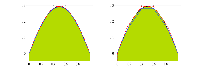
Refer to caption
Figure 5: The inner and outer approximations of the lower image 𝒟𝒟\mathcal{D} provided by Algorithm 2 (left) and its alternative (right).
Table 1: Computational data for Example 5.1
ϵitalic-ϵ\epsilon alg. / variant ##\# opt. ##\# vert. enum. |𝒳¯|¯𝒳\left|\bar{\mathcal{X}}\right| |𝒯¯|¯𝒯\left|\bar{\mathcal{T}}\right| |𝒳¯alt|subscript¯𝒳𝑎𝑙𝑡\left|\bar{\mathcal{X}}_{alt}\right| |𝒯¯alt|subscript¯𝒯𝑎𝑙𝑡\left|\bar{\mathcal{T}}_{alt}\right| time (s)
0.010.010.01 1 / break 171717 999 171717 171717 888 999 8.378.378.37
1 / no break 171717 555 171717 171717 888 999 8.268.268.26
2 / break 191919 111111 171717 171717 888 101010 8.928.928.92
2 / no break 191919 666 171717 171717 888 101010 8.858.858.85
0.0010.0010.001 1 / break 454545 232323 454545 454545 222222 232323 21.1821.1821.18
1 / no break 454545 777 454545 454545 222222 232323 21.4021.4021.40
2 / break 434343 232323 414141 414141 202020 222222 20.2420.2420.24
2 / no break 434343 888 414141 414141 202020 222222 20.0020.0020.00
Example 5.2.

Consider the following problem with non-differentiable constraint function

minimize Γ(x)=((x13)2+(x21)2(x11)2+(x21)2) with respect to +2minimize Γ𝑥binomialsuperscriptsubscript𝑥132superscriptsubscript𝑥212superscriptsubscript𝑥112superscriptsubscript𝑥212 with respect to subscriptsubscriptsuperscript2absent\displaystyle\text{minimize~{}~{}}\Gamma(x)=\binom{(x_{1}-3)^{2}+(x_{2}-1)^{2}}{(x_{1}-1)^{2}+(x_{2}-1)^{2}}\text{~{}with respect to~{}}\leq_{\mathbb{R}^{2}_{+}}
subject to |x1|+2|x2|2.subject to subscript𝑥12subscript𝑥22\displaystyle\text{subject to~{}}|x_{1}|+2|x_{2}|\leq 2.

The ordering cone is C=+2𝐶subscriptsuperscript2C=\mathbb{R}^{2}_{+}, and we fix c1=[1,0]T,c=[1,1]Tformulae-sequencesuperscript𝑐1superscript10𝑇𝑐superscript11𝑇c^{1}=[1,0]^{T},c=[1,1]^{T} as before. This example is taken from [7], and it was used as an example which can not be solved by the algorithm provided in [7]. Since we do not assume differentiability in order to use the algorithms provided here, the example can be solved. Figure 6 shows the approximations of the upper and lower images generated by Algorithm 1, where the approximation error ϵitalic-ϵ\epsilon is taken as 0.010.010.01. Computational data regarding this example can be seen in Table 2.
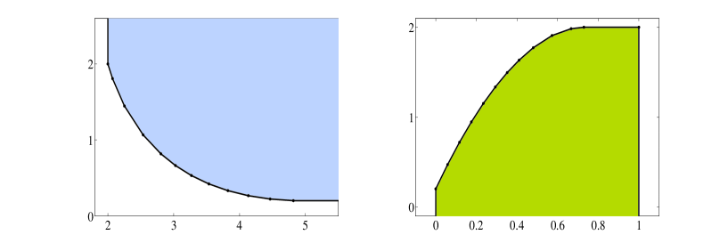
Refer to caption
Figure 6: The outer approximation of the upper image (left) and the inner approximation of the lower image (right) by Algorithm 1 for ϵ=0.01italic-ϵ0.01\epsilon=0.01 for Example 5.2.
Table 2: Computational data for Example 5.2
ϵitalic-ϵ\epsilon alg. / variant ##\# opt. ##\# vert. enum. |𝒳¯|¯𝒳\left|\bar{\mathcal{X}}\right| |𝒯¯|¯𝒯\left|\bar{\mathcal{T}}\right| |𝒳¯alt|subscript¯𝒳𝑎𝑙𝑡\left|\bar{\mathcal{X}}_{alt}\right| |𝒯¯alt|subscript¯𝒯𝑎𝑙𝑡\left|\bar{\mathcal{T}}_{alt}\right| time (s)
0.010.010.01 1 / break 252525 131313 242424 252525 121212 131313 16.5216.5216.52
1 / no break 252525 666 242424 252525 121212 131313 15.1815.1815.18
2 / break 272727 151515 252525 252525 121212 141414 17.5917.5917.59
2 / no break 272727 777 252525 252525 121212 141414 17.3917.3917.39
0.0010.0010.001 1 / break 555555 282828 545454 555555 272727 282828 33.2933.2933.29
1 / no break 555555 777 545454 555555 272727 282828 33.3133.3133.31
2 / break 515151 272727 494949 494949 242424 262626 32.1232.1232.12
2 / no break 515151 888 494949 494949 242424 262626 31.4031.4031.40
Example 5.3.

Consider the following problem

minimize Γ(x)=(ex1+ex4,ex2+ex5,ex3+ex6)T with respect to +3minimize Γ𝑥superscriptsuperscript𝑒subscript𝑥1superscript𝑒subscript𝑥4superscript𝑒subscript𝑥2superscript𝑒subscript𝑥5superscript𝑒subscript𝑥3superscript𝑒subscript𝑥6𝑇 with respect to subscriptsubscriptsuperscript3absent\displaystyle\text{minimize~{}~{}}\Gamma(x)=(e^{x_{1}}+e^{x_{4}},\;e^{x_{2}}+e^{x_{5}},\;e^{x_{3}}+e^{x_{6}})^{T}\text{~{}with respect to }\leq_{\mathbb{R}^{3}_{+}}
subject to x1+x2+x30subject to subscript𝑥1subscript𝑥2subscript𝑥30\displaystyle\text{subject to~{}~{}}x_{1}+x_{2}+x_{3}\geq 0
3x1+6x2+3x3+4x4+x5+4x603subscript𝑥16subscript𝑥23subscript𝑥34subscript𝑥4subscript𝑥54subscript𝑥60\displaystyle\hskip 55.48277pt3x_{1}+6x_{2}+3x_{3}+4x_{4}+x_{5}+4x_{6}\geq 0
3x1+x2+x3+2x4+4x5+4x60.3subscript𝑥1subscript𝑥2subscript𝑥32subscript𝑥44subscript𝑥54subscript𝑥60\displaystyle\hskip 55.48277pt3x_{1}+x_{2}+x_{3}+2x_{4}+4x_{5}+4x_{6}\geq 0.

We fix c1=[1,0,0]Tsuperscript𝑐1superscript100𝑇c^{1}=[1,0,0]^{T}, c2=[0,1,0]Tsuperscript𝑐2superscript010𝑇c^{2}=[0,1,0]^{T}, and c=[1,1,1]T𝑐superscript111𝑇c=[1,1,1]^{T}. Note that Assumptions 4.1 (b)-(d) hold, however the feasible region is not compact. Recall that one can still use the algorithms as long as the scalar problems have optimal solutions and in case the algorithms terminate, compare Remarks 3. and 4. in Section 4.3. We employ the convex optimization solver CVX, which detects whether the scalar problems are infeasible or unbounded, but not necessarily the case where a solution does not exist. If we apply Algorithm 2 to this example, for the unit vectors w=ei𝑤superscript𝑒𝑖w=e^{i} (i=1,2,3𝑖123i=1,2,3), the solver does not detect that (P(w)1{}_{1}(w)) does not have a solution and returns an approximate solution x𝑥x, where Γ(x)normΓ𝑥\left\|\Gamma(x)\right\| is very large. By numerical inaccuracy, we cannot ensure that the hyperplane H(Γ(x))superscript𝐻Γ𝑥H^{*}(\Gamma(x)) according to Proposition 4.13 is non-vertical. This is the reason why the dual algorithm does not work for this example. However we can still use Algorithm 1. Figure 7 shows the outer approximations to the upper image generated by Algorithm 1 with approximation errors 0.10.10.1 and 0.050.050.05. The graphics have been generated by JavaView111by Konrad Polthier, http://www.javaview.de. The numerical results can be seen in Table 3. This is an example where the algorithm proposed in [7] does not terminate for certain ϵ>0italic-ϵ0\epsilon>0 and pint𝒫𝑝int𝒫p\in{\rm int\,}\mathcal{P} (see [7]) due to a different measure for the approximation error.
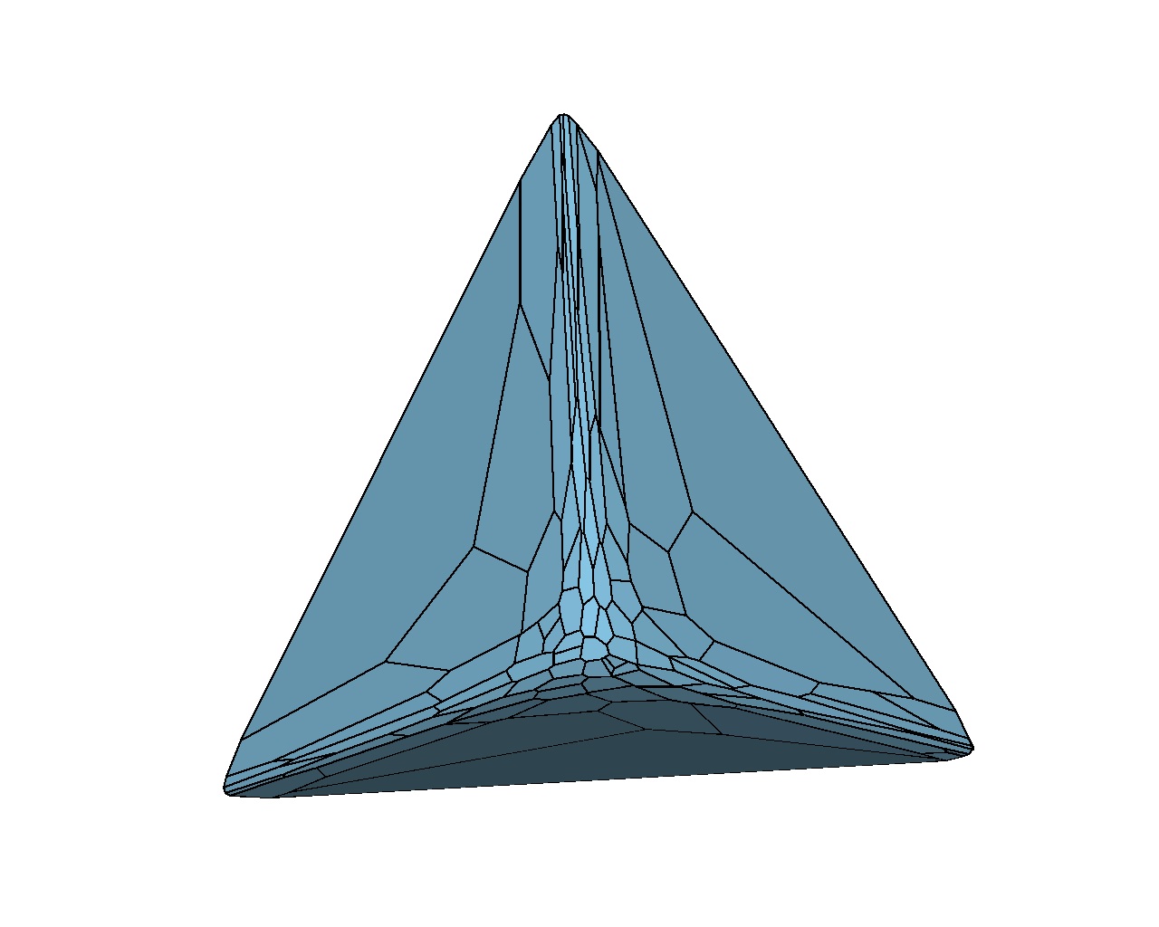
Refer to caption
Refer to caption
Refer to caption
Refer to caption
Figure 7: The outer approximation of the upper image 𝒫𝒫\mathcal{P} for Example 5.3 by Algorithm 1; displayed: y𝒫𝑦𝒫y\in\mathcal{P} with y1+y2+y336subscript𝑦1subscript𝑦2subscript𝑦336y_{1}+y_{2}+y_{3}\leq 36; top left: ‘break’, ϵ=0.1italic-ϵ0.1\epsilon=0.1; top right: ‘no break’, ϵ=0.1italic-ϵ0.1\epsilon=0.1; bottom left: ‘break’, ϵ=0.05italic-ϵ0.05\epsilon=0.05; bottom right: ‘no break’, ϵ=0.05italic-ϵ0.05\epsilon=0.05.
Table 3: Computational data for Example 5.3
ϵitalic-ϵ\epsilon alg. / variant ##\# opt. ##\# vert. enum. |𝒳¯|¯𝒳\left|\bar{\mathcal{X}}\right| |𝒯¯|¯𝒯\left|\bar{\mathcal{T}}\right| |𝒳¯alt|subscript¯𝒳𝑎𝑙𝑡\left|\bar{\mathcal{X}}_{alt}\right| |𝒯¯alt|subscript¯𝒯𝑎𝑙𝑡\left|\bar{\mathcal{T}}_{alt}\right| time (s)
0.10.10.1 1 / break 107107107 343434 107107107 107107107 727272 353535 284.68284.68284.68
1 / no break 133133133 777 133133133 133133133 878787 464646 355.29355.29355.29
0.050.050.05 1 / break 232232232 727272 231231231 232232232 158158158 737373 670.55670.55670.55
1 / no break 328328328 888 328328328 328328328 222222222 106106106 906.91906.91906.91
Example 5.4.

In this example we study the calculation of set-valued convex risk measures. It is known that polyhedral set-valued convex risk measures can be calculated by Benson’s algorithm for LVOPs (see [19, 12, 11]). Here, we show that (non-polyhedral) set-valued convex risk measures can be calculated approximately using the algorithms provided here. Consider a financial market consisting of d𝑑d assets, which can be traded at discrete time t=0,1,,T𝑡01𝑇t=0,1,\ldots,T. Let (Ω,,()t=0T,)Ωsuperscriptsubscript𝑡0𝑇(\Omega,\mathcal{F},(\mathcal{F})_{t=0}^{T},\mathbb{P}) be a finite probability space, where Ω={ω1,,ωN}Ωsubscript𝜔1subscript𝜔𝑁\Omega=\{\omega_{1},\ldots,\omega_{N}\}, (ωi)=pisubscript𝜔𝑖subscript𝑝𝑖\mathbb{P}(\omega_{i})=p_{i} such that pi(0,1]subscript𝑝𝑖01p_{i}\in(0,1], and =Tsubscript𝑇\mathcal{F}=\mathcal{F}_{T}. Assume that the market is defined by the tsubscript𝑡\mathcal{F}_{t} adapted process (Kt)t=0Tsuperscriptsubscriptsubscript𝐾𝑡𝑡0𝑇(K_{t})_{t=0}^{T} of solvency cones, which represent the exchange rates and proportional transaction costs between the d𝑑d assets (see [17]). Note that Kt(ωn)subscript𝐾𝑡subscript𝜔𝑛K_{t}(\omega_{n}) is a polyhedral closed convex cone, with +dKt(ωn)dsubscriptsuperscript𝑑subscript𝐾𝑡subscript𝜔𝑛superscript𝑑\mathbb{R}^{d}_{+}\subseteq K_{t}(\omega_{n})\neq\mathbb{R}^{d} for t=0,,T𝑡0𝑇t=0,\ldots,T, n=1,,N𝑛1𝑁n=1,\ldots,N.

In this setting Ararat, Rudloff, and Hamel [1] consider set-valued shortfall risk measures on Ld=Ld(Ω,T,)subscriptsuperscript𝐿𝑑subscriptsuperscript𝐿𝑑Ωsubscript𝑇L^{\infty}_{d}=L^{\infty}_{d}(\Omega,\mathcal{F}_{T},\mathbb{P}), the linear space of the equivalence classes of Tsubscript𝑇\mathcal{F}_{T}-measurable, \mathbb{P}-a.s. bounded, d𝑑d-dimensional random vectors. Let l=(l1,,ld):Ldd:𝑙subscript𝑙1subscript𝑙𝑑subscriptsuperscript𝐿𝑑superscript𝑑l=(l_{1},\ldots,l_{d}):L^{\infty}_{d}\rightarrow\mathbb{R}^{d} be a loss function such that li:Ld:subscript𝑙𝑖subscriptsuperscript𝐿𝑑l_{i}:L^{\infty}_{d}\rightarrow\mathbb{R} is convex and increasing for i=1,,d𝑖1𝑑i=1,\ldots,d. We consider here the one-period case T=1𝑇1T=1 only. It was shown that the market extension of the set-valued l𝑙l-shortfall risk measure is

Rmar(X)superscript𝑅𝑚𝑎𝑟𝑋\displaystyle R^{mar}(X) ={md:𝔼[l(X+Ym+y)]{x0}A,YLd(K1),yK0},absentconditional-set𝑚superscript𝑑formulae-sequence𝔼delimited-[]𝑙𝑋𝑌𝑚𝑦subscript𝑥0𝐴formulae-sequence𝑌subscriptsuperscript𝐿𝑑subscript𝐾1𝑦subscript𝐾0\displaystyle=\{m\in\mathbb{R}^{d}:\>\mathbb{E}\left[l(-X+Y-m+y)\right]\in\{x_{0}\}-A,\>\>Y\in L^{\infty}_{d}(K_{1}),\>\>y\in K_{0}\},

where XLd𝑋subscriptsuperscript𝐿𝑑X\in L^{\infty}_{d}, Ld(K1):={ZLd:ZK1-a.s.}assignsubscriptsuperscript𝐿𝑑subscript𝐾1conditional-set𝑍subscriptsuperscript𝐿𝑑𝑍subscript𝐾1-a.s.L^{\infty}_{d}(K_{1}):=\{Z\in L^{\infty}_{d}:\;Z\in K_{1}\;\mathbb{P}\text{-a.s.}\}, A𝐴A is a convex upper closed set, that is cl(conv(A++d))=Aclconv𝐴subscriptsuperscript𝑑𝐴{\rm cl\,}({\rm conv\,}(A+\mathbb{R}^{d}_{+}))=A, and 0bdA0bd𝐴0\in{\rm bd\,}A. It is shown in [1] that Rmar(X)=Rmar(X)+K0superscript𝑅𝑚𝑎𝑟𝑋superscript𝑅𝑚𝑎𝑟𝑋subscript𝐾0R^{mar}(X)=R^{mar}(X)+K_{0}. For a given random vector X𝑋X, the set Rmar(X)superscript𝑅𝑚𝑎𝑟𝑋R^{mar}(X) is the upper image of the following vector optimization problem

minimize md with respect to K0minimize 𝑚superscript𝑑 with respect to subscriptsubscript𝐾0absent\displaystyle\text{minimize~{}~{}}m\in\mathbb{R}^{d}\text{~{}~{}~{}with respect to~{}}\leq_{K_{0}}
subject to 𝔼[l(X+Ym+y)]{x0}A,subject to 𝔼delimited-[]𝑙𝑋𝑌𝑚𝑦subscript𝑥0𝐴\displaystyle\text{subject to~{}~{}}\mathbb{E}\left[l(-X+Y-m+y)\right]\in\{x_{0}\}-A,
YLd(K1),yK0,formulae-sequence𝑌subscriptsuperscript𝐿𝑑subscript𝐾1𝑦subscript𝐾0\displaystyle\qquad\qquad\quad Y\in L^{\infty}_{d}(K_{1}),\;y\in K_{0},

and thus can be approximated by the algorithms presented in this paper, whenever the set A𝐴A is polyhedral, say A={zd:(a1)Tzb1,,(as)Tzbs}𝐴conditional-set𝑧superscript𝑑formulae-sequencesuperscriptsuperscript𝑎1𝑇𝑧subscript𝑏1superscriptsuperscript𝑎𝑠𝑇𝑧subscript𝑏𝑠A=\{z\in\mathbb{R}^{d}:(a^{1})^{T}z\geq b_{1},\ldots,(a^{s})^{T}z\geq b_{s}\}. Then, the constraint 𝔼[l(X+Ym+y)]{x0}A𝔼delimited-[]𝑙𝑋𝑌𝑚𝑦subscript𝑥0𝐴\mathbb{E}\left[l(-X+Y-m+y)\right]\in\{x_{0}\}-A can be written as

gi(Y,y,m):=(ai)T[x0+𝔼[l(X+Ym+y)]]bi,i=1,,s.formulae-sequenceassignsubscript𝑔𝑖𝑌𝑦𝑚superscriptsuperscript𝑎𝑖𝑇delimited-[]subscript𝑥0𝔼delimited-[]𝑙𝑋𝑌𝑚𝑦subscript𝑏𝑖𝑖1𝑠g_{i}(Y,y,m):=(a^{i})^{T}\big{[}-x_{0}+\mathbb{E}\left[l(-X+Y-m+y)\right]\big{]}\leq-b_{i},\>\>\>i=1,\ldots,s.

As A𝐴A is upper closed we have ai+dsuperscript𝑎𝑖subscriptsuperscript𝑑a^{i}\in\mathbb{R}^{d}_{+}, which implies that gisubscript𝑔𝑖g_{i} is convex. It is clear that the second and third set of constraints, and the objective function are linear. Thus, the problem is a CVOP with ordering cone K0subscript𝐾0K_{0}. Similar to Example 5.3, Assumptions 4.1 (b)-(d) hold, however the feasible region is not compact as md𝑚superscript𝑑m\in\mathbb{R}^{d} is not bounded. Remarks 3. and 4. in Section 4.3 explain the implications of that for the algorithms.

For a numerical example, set d=4𝑑4d=4, T=1𝑇1T=1, |Ω|=8Ω8|\Omega|=8, and pn=0.125subscript𝑝𝑛0.125p_{n}=0.125 for n=1,,8𝑛18n=1,\ldots,8. We fix K^04×12subscript^𝐾0superscript412\hat{K}_{0}\in\mathbb{R}^{4\times 12}, and K^T(ωn)4×12subscript^𝐾𝑇subscript𝜔𝑛superscript412\hat{K}_{T}(\omega_{n})\in\mathbb{R}^{4\times 12}, whose columns are the generating vectors of corresponding solvency cones K0subscript𝐾0K_{0} and KT(ωn)subscript𝐾𝑇subscript𝜔𝑛K_{T}(\omega_{n}), n=1,,8𝑛18n=1,\ldots,8. Let x0=04subscript𝑥00superscript4x_{0}=0\in\mathbb{R}^{4}, and A={z4:eTz0}𝐴conditional-set𝑧superscript4superscript𝑒𝑇𝑧0A=\{z\in\mathbb{R}^{4}:e^{T}z\geq 0\}, where e𝑒e is the vector of ones. We calculate Rmar(X)superscript𝑅𝑚𝑎𝑟𝑋R^{mar}(X) for XL4𝑋subscriptsuperscript𝐿4X\in L^{\infty}_{4} being the payoff of an outperformance option. The vector-valued loss function is taken as l(x)=(l1,,l4)T𝑙𝑥superscriptsubscript𝑙1subscript𝑙4𝑇l(x)=(l_{1},\ldots,l_{4})^{T}, with li(x)=exi1subscript𝑙𝑖𝑥superscript𝑒subscript𝑥𝑖1l_{i}(x)=e^{x_{i}}-1.

We modeled the problem as a CVOP, where there are 444 objectives, 112112112 decision variables, and 109109109 constraints. The ordering cone is K0+4subscriptsuperscript4subscript𝐾0K_{0}\supsetneq\mathbb{R}^{4}_{+} with 121212 generating vectors, and we fix c1=[1,0,0,0]Tsuperscript𝑐1superscript1000𝑇c^{1}=[1,0,0,0]^{T}, c2=[0,1,0,0]Tsuperscript𝑐2superscript0100𝑇c^{2}=[0,1,0,0]^{T}, c3=[0,0,1,0]Tsuperscript𝑐3superscript0010𝑇c^{3}=[0,0,1,0]^{T}, and c=[1,1,1,1]T𝑐superscript1111𝑇c=[1,1,1,1]^{T}. We try both algorithms to solve the problem for different values of ϵitalic-ϵ\epsilon. It turns out that the solver fails to solve (P(v)2{}_{2}(v)) for some of the vertices of the current outer approximation 𝒫ksubscript𝒫𝑘\mathcal{P}_{k} of the upper image. However, (P(w)1{}_{1}(w)) can be solved for each w=w(t)𝑤𝑤𝑡w=w(t), for the vertices t𝑡t of the outer approximations 𝒟ksubscript𝒟𝑘\mathcal{D}_{k} of the lower image. Thus, Algorithm 2 provides a finite weak ϵitalic-ϵ\epsilon-solution to (P), and a finite ϵitalic-ϵ\epsilon-solution to (D). Also, we only use the variant with ‘break’ as it turns out that it can solve the problem in less time compared to the variant without ‘break’. Table 4 shows some computational data of Algorithm 2.

Table 4: Computational data for Example 5.4
ϵitalic-ϵ\epsilon alg. / variant ##\# opt. ##\# vert. enum. |𝒳¯|¯𝒳\left|\bar{\mathcal{X}}\right| |𝒯¯|¯𝒯\left|\bar{\mathcal{T}}\right| |𝒳¯alt|subscript¯𝒳𝑎𝑙𝑡\left|\bar{\mathcal{X}}_{alt}\right| |𝒯¯alt|subscript¯𝒯𝑎𝑙𝑡\left|\bar{\mathcal{T}}_{alt}\right| time (s)
0.010.010.01 2 / break 152152152 222222 151151151 148148148 191919 132132132 3046.53046.53046.5
0.0050.0050.005 2 / break 255255255 383838 254254254 249249249 353535 219219219 4941.64941.64941.6
0.0010.0010.001 2 / break 143314331433 188188188 142914291429 141014101410 185185185 124712471247 267062670626706
0.00050.00050.0005 2 / break 310931093109 380380380 310731073107 307530753075 377377377 273127312731 583975839758397

References

  • [1] Ç. Ararat, A. H. Hamel, and B. Rudloff. Set-valued shortfall and divergence risk measures. submitted, 2014.
  • [2] H. P. Benson. An outer approximation algorithm for generating all efficient extreme points in the outcome set of a multiple objective linear programming problem. Journal of Global Optimization, 13:1–24, 1998.
  • [3] D. Bremner, K. Fukuda, and A. Marzetta. Primal-dual methods for vertex and facet enumeration. Discrete Computational Geometry, 20(3):333–357, 1998.
  • [4] L. Csirmaz. Using multiobjective optimization to map the entropy region of four random variables. preprint, 2013. http://eprints.renyi.hu/66/2/globopt.pdf.
  • [5] Inc. CVX Research. CVX: Matlab software for disciplined convex programming, version 2.0 beta., September 2012.
  • [6] M. Ehrgott, A. Löhne, and L. Shao. A dual variant of Benson’s outer approximation algorithm. Journal Global Optimization, 52(4):757–778, 2012.
  • [7] M. Ehrgott, L. Shao, and A. Schöbel. An approximation algorithm for convex multi-objective programming problems. Journal of Global Optimization, 50(3):397–416, 2011.
  • [8] M. Ehrgott and M. M. Wiecek. Multiobjective programming. In J. Figueira, S. Greco, and M. Ehrgott, editors, Multicriteria Decision Analysis: State of the Art Surveys, pages 667–722. Springer Science + Business Media, 2005.
  • [9] M. C. Grant and S. P. Boyd. Graph implementations for nonsmooth convex programs. In V. Blondel, S. Boyd, and H. Kimura, editors, Recent Advances in Learning and Control, volume 371 of Lecture Notes in Control and Information Sciences, pages 95–110. Springer, London, 2008.
  • [10] A. H. Hamel and A. Löhne. Lagrange duality in set optimization. Journal of Optimization Theory and Applications, 2013, DOI: 10.1007/s10957-013-0431-4.
  • [11] A. H. Hamel, A. Löhne, and B. Rudloff. A Benson type algorithm for linear vector optimization and applications. Journal of Global Optimization, 2013, DOI: 10.1007/s10898-013-0098-2.
  • [12] A. H. Hamel, B. Rudloff, and M. Yankova. Set-valued average value at risk and its computation. Mathematics and Financial Economics, 7(2):229–246, 2013.
  • [13] F. Heyde. Geometric duality for convex vector optimization problems. Journal of Convex Analysis, 20(3):813–832, 2013.
  • [14] F. Heyde and A. Löhne. Geometric duality in multiple objective linear programming. SIAM Journal of Optimization, 19(2):836–845, 2008.
  • [15] F. Heyde and A. Löhne. Solution concepts in vector optimization: a fresh look at an old story. Optimization, 60(12):1421–1440, 2011.
  • [16] J. Jahn. Vector Optimization - Theory, Applications, and Extensions. Springer, 2004.
  • [17] Y. M. Kabanov. Hedging and liquidation under transaction costs in currency markets. Finance and Stochastics, 3:237–248, 1999.
  • [18] A. Löhne. Vector Optimization with Infimum and Supremum. Springer, 2011.
  • [19] A. Löhne and B. Rudloff. An algorithm for calculating the set of superhedging portfolios in markets with transaction costs. International Journal of Theoretical and Applied Finance, Forthcoming, 2013.
  • [20] D. Luc. Theory of Vector Optimization, volume 319 of Lecture Notes in Economics and Mathematical Systems. Springer Verlag, 1989.
  • [21] R. T. Rockafellar. Convex Analysis. Princeton University Press, 1970.
  • [22] S. Ruzika and M. M. Wiecek. Approximation methods in multiobjective programming. Journal of Optimization Theory and Applications, 126(3):473–501, September 2005.
  • [23] L. Shao and M. Ehrgott. Approximately solving multiobjective linear programmes in objective space and an application in radiotherapy treatment planning. Mathematical Methods of Operations Research, 68(2):257–276, 2008.
  • [24] L. Shao and M. Ehrgott. Approximating the nondominated set of an MOLP by approximately solving its dual problem. Mathematical Methods of Operations Research, 68(3):469–492, 2008.