The Generalized Mean Information Coefficient
Abstract
Objective: Reshef & Reshef recently published a paper in which they present a method called the Maximal Information Coefficient (MIC) that can detect all forms of statistical dependence between pairs of variables as sample size goes to infinity. While this method has been praised by some, it has also been criticized for its lack of power in finite samples. We seek to modify MIC so that it has higher power in detecting associations for limited sample sizes.
Methods: Here we present the Generalized Mean Information Coefficient (GMIC), a generalization of MIC which incorporates a tuning parameter that can be used to modify the complexity of the association favored by the measure. We define GMIC and prove it maintains several key asymptotic properties of MIC. Its increased power over MIC is demonstrated using a simulation of eight different functional relationships at sixty different noise levels. The results are compared to the Pearson correlation, distance correlation, and MIC.
Results: Simulation results suggest that while generally GMIC has slightly lower power than the distance correlation measure, it achieves higher power than MIC for many forms of underlying association. For some functional relationships, GMIC surpasses all other statistics calculated. Preliminary results suggest choosing a moderate value of the tuning parameter for GMIC will yield a test that is robust across underlying relationships.
Conclusion: GMIC is a promising new method that mitigates the power issues suffered by MIC, at the possible expense of equitability. Nonetheless, distance correlation was in our simulations more powerful for many forms of underlying relationships. At a minimum, this work motivates further consideration of maximal information-based nonparametric exploration (MINE) methods as statistical tests of independence.
I. Introduction.
Reshef & Reshef recently published a paper called “Detecting Novel Associations in Large Data Sets”, in which they present the Maximal Information Coefficient (MIC). This statistic is able to detect many forms of association between pairs of variables, including all functional and a wide range of non-functional relationships[1]. Additionally, MIC is a provably equitable statistic, in the senes that it gives approximately equal scores to different relationships at equal noise levels[1, 2]. Nonetheless, the method has its shortcomings. Shortly after publication, Simon & Tibshirani published an analysis which showed that, as a test of association, MIC performed worse in terms of power than several other tests of association for many realistic functional forms[3]. It is even sometimes less powerful than the Pearson correlation. Simon notes that basic statistical experience suggests testing against such a wide range of alternatives should reduce power in many realistic situations. While MIC’s ability to detect the superposition of functions and other complex relationships is a novel and exciting development, most researchers want to detect far simpler relationships in their data. The authors of the original MINE paper responded to the criticism of Simon & Tibshirani and others in a prepared statement on Andrew Gelman’s website by arguing that the main contribution of MIC as a statistic is its equitability, even at the cost of statistical power [4].
In this paper we focus on statistical power rather than equitability. We present the Generalized Mean Information Coefficient (GMIC), a generalization of MIC which incorporates a tuning parameter that can be used to modify the complexity of the association favored by the measure in a controlled way. Our modification falls into the class of maximal information-based nonparametric exploration (MINE) statistics presented in the original publication. Specifically, we aim to:
-
1.
Introduce GMIC.
-
2.
Prove that our generalization asymptotically detects the same class of associations as MIC.
-
3.
Provide intuition as to why our generalization should have higher power in most realistic situations.
-
4.
Provide simulation evidence supporting our claims.
-
5.
Compare GMIC to other association statistics using simulation.
II. Methods.
1. Maximal Information Coefficient.
Using mutual information (MI) as a foundation, Reshef & Reshef propose MIC. Before our discussion of MIC, we review the statistic. Suppose is a set of i.i.d. random variables drawn from some distribution . We let and . Let represent the estimated mutual information obtained by placing into the bins defined by , a grid with columns and rows. That is, . See Fig. 1 in the original publication for a graphical interpretation of this procedure. Then for all integers :
where is an infinite matrix and represents the base 2 logarithm. We start the row and column indexing at for convenience. Reshef & Reshef call the characteristic matrix. Note that for all , and thus . Then MIC is given by:
where , , is the maximal grid size necessary to control the type I error rate asymptotically. Reshef & Reshef suggest letting . Clearly . An additional desirable property of MIC is that it only depends on the rank-order of and . Thus if we compute significance by permutation, we can precompute significance cutoffs for fixed sample sizes and values of .
While exact values of the characteristic matrix can be computed, the space of grids to be searched grows exponentially in . To make running the algorithm feasible on large data sets, Reshef & Reshef propose a dynamic programming algorithm which provides a close approximation to the characteristic matrix. We refer to the measure that results from using this matrix .
In the supplementary materials to the main paper, Reshef & Reshef prove that has a number of desirable properties. Because we will use these results to prove that our generalization has similar properties, we restate the results here. For simplicity, here we assume that to avoid restating conditions on . The original publication shows that:
-
•
If and are statistically independent, then in probability as .
-
•
If and are not statistically independent, then there exists a constant such that almost surely as .
-
•
Let be a nowhere constant function on and be a continuous random variable. Then as almost surely.
- •
Note that we are only guaranteed that the approximate algorithm converges to zero in probability for statistically independent random variables and not that converges to zero in probability.
Thus MIC satisfies many desirable properties for an estimator. In the next section, we briefly discuss one of the MINE statistcs introduced by Reshef & Reshef to motivate our proposal of a generalization of MIC which prefers simpler association relationships.
2. Minimum Cell Number.
To summarize the complexity of an association, Reshef & Reshef propose the minimum cell number (MCN):
Where the parameter is chosen based on the desired level of robustness. Larger values of the MCN indicate a complex association, while smaller values indicate a simpler association. As can be seen in Table S1 in the Supplementary Online Materials of the original paper, many realistic associations will tend to have lower MCN scores. In the next section we propose a method which penalizes complex associations in finite samples while maintaining several of the desirable asymptotic properties of MIC.
A. Generalized Mean Information Coefficient.
1. GMIC Definition.
Before introducing the GMIC statistic, we define the maximal characteristic matrix as:
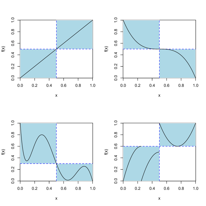
for all . That is, is the maximal normalized mutual information which can be achieved using grid sizes no larger than . This processing step is needed for our theoretical results about asymptotically detecting all forms of statistical dependence to hold. Note that can be computed efficiently from the characteristic matrix returned by the current MIC implementation. See Figure 1 to see how the maximal characteristic matrix differs from the characteristic matrix in two fabricated examples.
We define as:
where is a tuning parameter in and . We use the convention that for all . We take to denote the minimum and to denote the maximum since these values hold in the limit.
Note that is a generalized mean. For we take to denote the geometric mean of because this relation holds in the limit as . The generalized mean inequality then guarantees that for all (see 3.2.4 in [6]). We denote the value of computed on the approximate maximal characteristic resulting from Reshef & Reshef’s algorithm as . The fact that shows that . In the special case of , .
We also denote as MinIC, standing for the Minimal Information Coefficient. When we invoke the generalized mean inequality in the proofs in the appendix we use the more direct to reference this when because it fits naturally into the generalized mean framework. Note that MinIC does not return the minimal value from the characteristic matrix , but rather the minimal value from the maximal characteristic matrix , i.e. .
Examining the definition of shows that the elements of are nondecreasing as increases. The characteristic matrix used by MIC, on the other hand, does not necessarily have this monotonic property (see Figure S7 in the supplementary online materials of[1]).
For , is similar to the MCN in that it takes into account how quickly (in terms of grid size) the characteristic matrix reaches its maximum. Unlike the MCN, also takes into account the overall magnitude of the characteristic matrix entries at grid sizes smaller than the grid size which maximizes . In general, for , can be viewed as a compromise between the value of the maximal mutual information attainable in a grid and the maximal mutual information attainable among all grids of size less than . That is, characteristic matrices with larger values of or which obtain their maximum at smaller grid sizes will in general achieve higher values of .
2. Properties of GMIC.
The monotonic nature of will allow us to prove several desirable asymptotic properties of GMIC. Specifically, we prove the following results:
-
•
Theorem 2. shows that the approximation algorithm for converges in probability to as for statistically independent random variables.
-
•
Theorem 2. shows that approaches some almost surely for statistically dependent random variables.
-
•
Theorem 2. gives a sufficient condition under which that approaches for all .
-
•
Corollary 1 shows that approaches for all noiseless monotonic relationships.
We first show that the approximation algorithm for converges in probability to as for statistically independent random variables. {restatable}apptheoremgmicindepzero Suppose is a set of continuous i.i.d. random variables where has support on and that is statistically independent of . Then in probability as for all . We now show that is bounded away from zero for statistically dependent random variables. {restatable}apptheoremgmicdepzeta Suppose is a set of continuous i.i.d. random variables where has support on and that and are statistically dependent. Then there exists some constant such that almost surely as . We now develop conditions under which approaches for all choices of the tuning parameter . Unsurprisingly, these conditions are stronger than the analogous conditions for . {restatable}apptheoremgmicone Suppose is a set of continuous i.i.d. random variables where has support on . Let and . Then in probability for all if one of the following two conditions holds for some and :
-
1.
and
-
2.
and
Figure 2 gives examples of relationships that satisfy the conditions of Theorem 2.. The next corollary shows that asymptotically approaches for monotonically increasing or decreasing functional relationships.
Corollary 1.
Suppose is a set of continuous i.i.d. random variables where is continuous with support on . Further suppose that almost surely for some noiseless monotonic, nowhere constant function . Then for all .
Sketch of proof.
Note that satisfies the conditions in Theorem 2.. ∎
3. Hypothesis Testing with GMIC.
We now consider hypothesis testing with . Suppose we wish to test the null distribution that and are statistically independent against the alternative that and are statistically dependent. Then a natural test is to reject the null hypothesis for large values of . Note that for the same reasons discussed in the MIC paper, GMIC is a rank-order statistic. For continuous random variables, rank ties occur with probability zero. Thus, as in the original MIC paper, we can compute significance by computing for fixed on draws from the permutation distribution. Trivially, note that we cannot use the null distribution of to compute the significance of for some . Thus we must compute separate empirical null distributions (though perhaps on the same Monte Carlo draws) for each of interest.
For a data set in which many variable pairs are of interest, Reshef & Reshef suggest controlling the false discovery rate [7]. We do not consider the multiple testing problem here.
4. Implementation.
B. Squared Pearson Correlation Coefficient.
We also compare GMIC with two existing association measures that do not belong to the MINE family of statistics. The first of these measures is given by the square of the Pearson correlation coefficient. Although a squared correlation of zero does not necessarily imply that and are independent, we use to test the hypothesis that and are statistically independent against the alternative that they are not because is commonly used to test this hypothesis in practice. Specifically, we reject for large values of . Nonetheless, we recognize that it is in fact inappropriate to use Pearson correlation coefficient to test this hypothesis (e.g. for the quadratic relationship in our simulation, see Section III.A.).
C. Distance Correlation.
The second existing association measure considered is distance correlation as proposed by Székely et al. in [10]. Specifically, they consider the parameter:
Where and are defined in Definition 2 of Székely et al. 2007. While we limit the discussion of distance correlation here, we note that it has the desirable property that if and only if and are independent. Conditions under which dCor is are given in Theorem 3 of the Székely et al. paper. To estimate , we use the empirical distance correlation given in Definition 5 of the Székely et al. paper.
We use the empirical distance correlation to test the null hypothesis that and are statistically independent against the alternative that they are not. Specifically we reject for large values of the empirical distance correlation.
For our simulations we use the R implementation of distance correlation in the energy package [11].
III. Data.
A. Simulation.
A simulation of eight different functional relationship was implemented to compare the power of each statistic considered. Specifically, we considered:
| (1) |
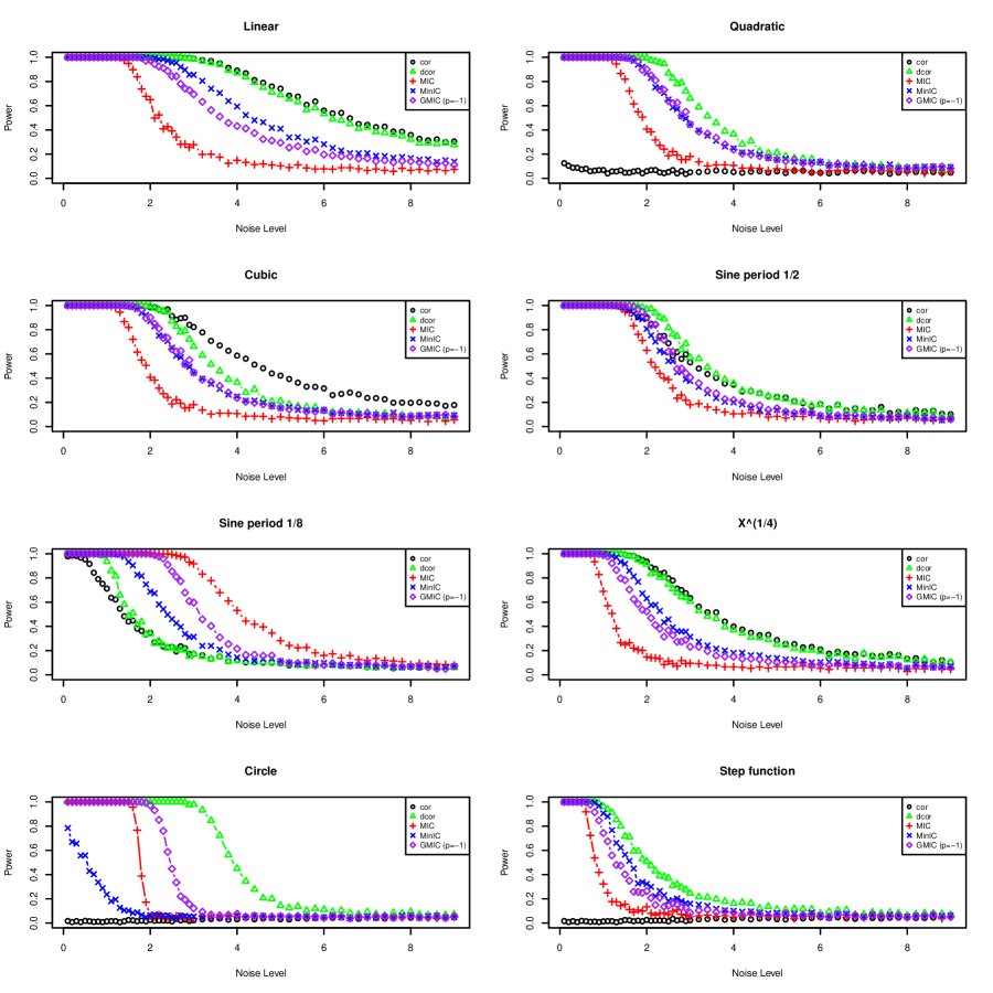
for . These functions were originally considered by Simon & Tibshirani to assess the statistical power of MIC [3]. Plots of all relationships are shown in Figure 3. One thousand runs were used to estimate each null and alternative distribution at observations and different noise levels. Like Simon and Tibshirani, we determined proper cutoffs for a level test using the percentile of from the marginal empirical distributions for each . That is, we sampled i.i.d. from Uniform, generated according to the functions in Equation 1 using , and sampled a separate i.i.d. Uniform. We then computed on both and . Power was calculated as the proportion of runs in the alternative distribution higher than the calculated cutoff from the null distribution . To analyze the performance of the GMIC under different values of the tuning parameter, the simulation was completed under approximately different values of :
In the figures for is referred to as MinIC and is referred to by its original name, MIC. Our consideration of smaller increments as we approached was due to our initial impression that the maximal power would be obtained at this value.
The limiting value approached by GMIC as under different values of the tuning parameter may vary for many noiseless relationships. Futhermore, the limiting value may depend on the form of the relationship. To analyze non-statistical interpretability in practice, we computed the sample mean of GMIC under three different tuning parameter values, namely , , , and compared to these values to the sample means of distance correlation and the squared Pearson’s correlation coefficient.
IV. Results.
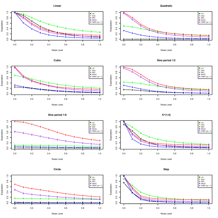
Figure 4 shows the power across noise levels for the various relationships with a sample size of 2000. Note that has higher power than MIC for all relationships except the high-frequency sine wave. MinIC has lower power for the high-frequency sine and circle relationships. Notably, the distance correlation statistic still outperforms both and MinIC for all but one relationship (high-frequency sine). It is also worth noting that while beats MinIC in terms of power for the sine period and circle relationships, the opposite holds true for the linear, , and step function relationships. For the quadratic, cubic, and sine period relationships, MinIC and have only slightly lower power than distance correlation across the various noise levels.
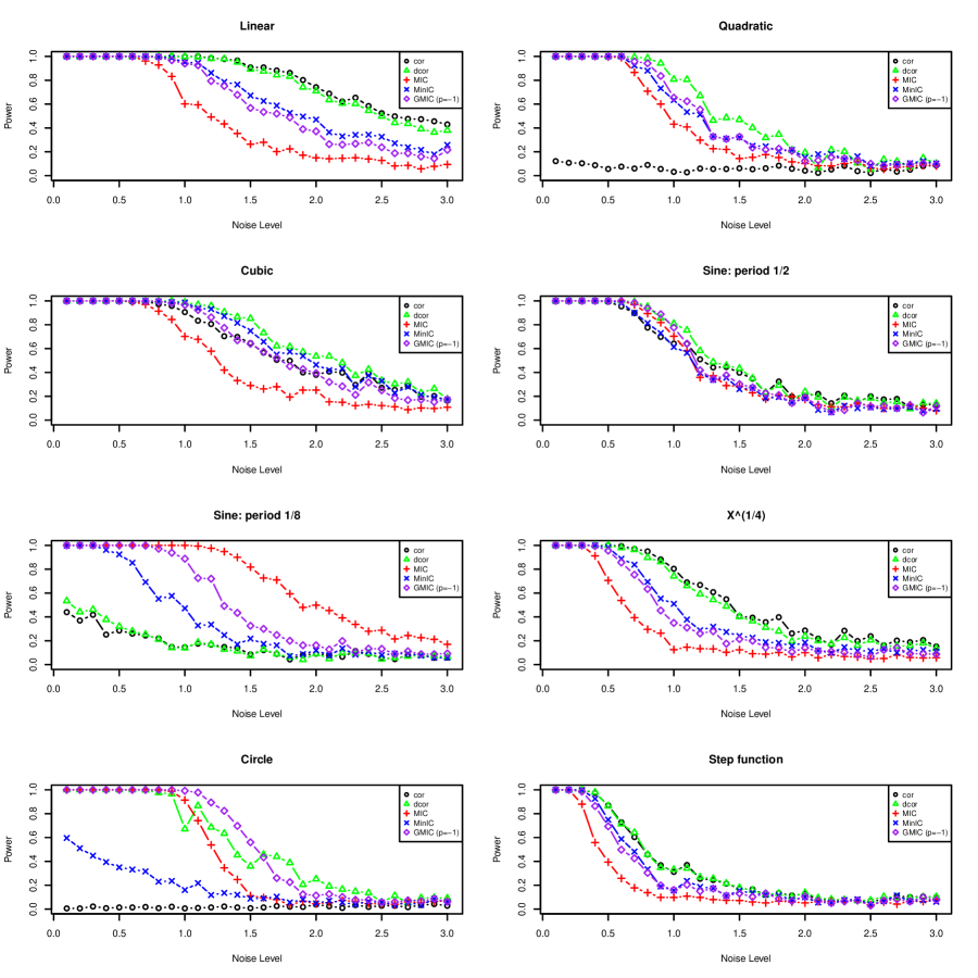
For comparison with the Simon & Tibshirani commentary, we also ran the simulation at a sample size of . The results, which appear in Figure 5, are similar to the results at .
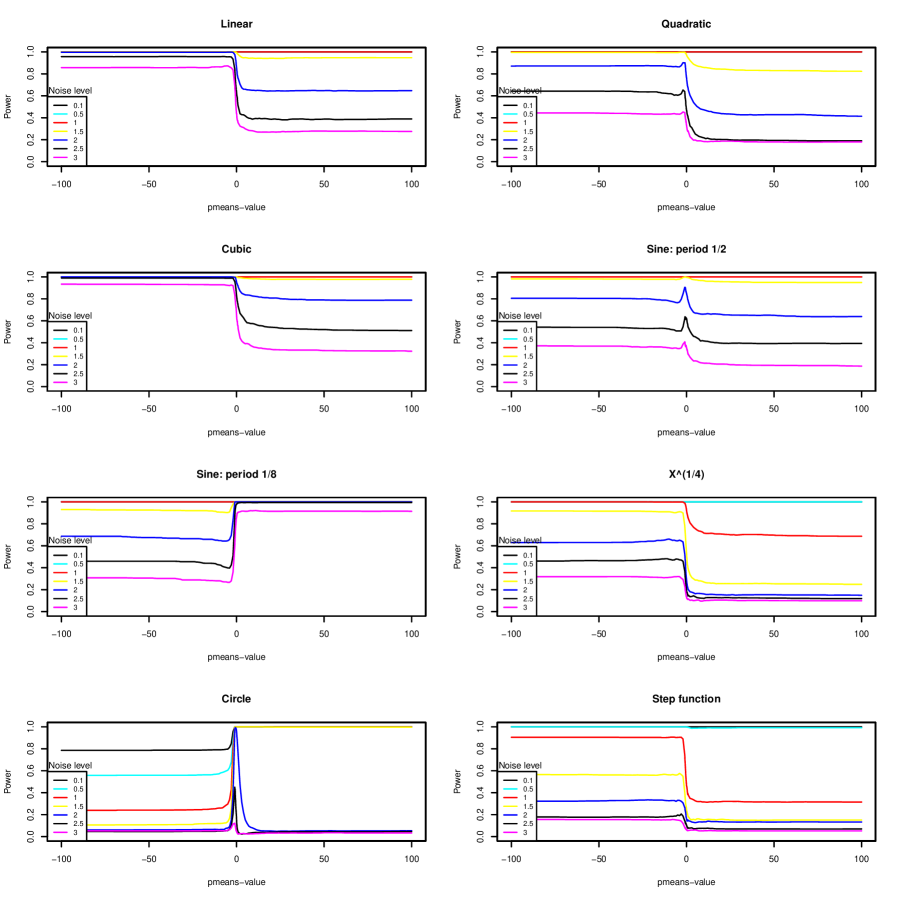
Figure 6 shows the power for GMIC at each of the approximately tuning parameter values, plotted at seven different noise levels. Interestingly, a sharp increase in the power occurs around for every relationship considered except for sine period . This is consistent with the results seen in Figure 4. The power tends to stays relatively constant at non-negative values. Note that a priori we believed that for some small would yield the most robust statistic. The choice to include instead of was made based on the results of Figure 6. We acknowledge that such a procedure may take away from the generalizability of the results to other relationships, and that further work is needed to find the best choice of the tuning parameter . Nonetheless, attained power close to that of in many situations as evidenced in Figure 6. Further work is needed to determine how to choose in a more general setting.
Figure 7 shows the sample mean of each statistic for the eight relationships of interest under the first noise levels as well as without noise. As expected, values for all statistics decrease as noise level increases. Whereas MIC should approach as grows at a noise level of zero for all relationships considered, we have no such guarantee for . Nonetheless, the sample mean of is close to the sample mean of MinIC across all relationships except the high-frequency sine and the circle. MinIC is considerably smaller than MIC and across all relationships except the step function and relationships. Under the linear association, all values approach as the noise level approaches .
Similarly, the distance correlation coefficient is noticeably lower in all the noiseless non-monotonic associations tested. Its sample mean is lower than (or equal to) the expected value of for every functional relationship considered.
V. Discussion.
The objective of this study was to develop and test a modification to MIC to increase its low statistical power. We have defined an alternative with GMIC and shown analytically that maintains many of the same nice properties that MIC possesses. We have also shown by simulation that there are many realistic settings in which our method performs better than MIC in terms of power for various values of the tuning parameter.
As is always the case, the introduction of a tuning parameter naturally leads to the question of which choice of is optimal in terms of some criterion, e.g. statistical power. Our initial belief was that the peak would occur at a value near , thereby approximately returning the geometric mean. The geometric mean was appealing because it (informally) represents the midpoint of , and thus seemed to offer a natural compromise between the extremes of MIC and MinIC. In Figure 6, we see that except for the high frequency sine wave, our power appears to be robust at approximately . Within the generalized mean framework, yields a harmonic mean of the maximal characteristic matrix. A more formal study should be conducted in order to verify that performs well at other sample sizes and for other realistic relationships. As stated earlier, for most of the relationships considered the power drops dramatically at non-negative values.
In simulation, largely outperforms MIC for most of the relationships tested. Nonetheless, distance correlation was clearly superior to all other methods considered in terms of power. Whereas has somewhat similar performance in the quadratic, cubic, and sine (period ) associations, the distance correlation still outperforms both GMIC and MinIC for all relationships except for the high frequency sine wave.
Practitioners may find equitability to be a valuable property. According to Reshef & Reshef, an equitable statistic is one that “should give similar scores to equally noisy relationships of different types” [1]. Equitability allows the user to easily interpret the strength of the bivariate association. Values close to 1 have very low variance in the assocation and values close to 0 have no association. Reshef & Reshef showed that MIC satisfies a particular equitability criterion. As of now, we do not have any equitability results for GMIC, nor do we expect that satisfies an equitability criterion analogous to the one satisfied by MIC.
Without equitability, interpretability may become an issue when testing across large numbers of pairwise associations. A significance level is less useful if one cannot differentiate between the complexity of the relationship and the underlying noise level implied by a coefficient estimate. allows for a natural trade-off between equitability and power, as larger values of the tuning parameter will tend towards MIC. If the desire is to gain power, the practitioner may choose a value for closer to .
While generally has more power than the MIC, there are still further advances needed. We now have a statistic that allows the user to trade equitability for more statistical power. We leave it to the reader to decide whether the trade is profitable. At a minimum, this work motiviates further consideration of MINE methods as statistical tests of independence.
Acknowledgements.
AL and LT would like to thank Sandrine Dudoit for valuable discussions. AL gratefully acknowledges the support of the Department of Defense (DoD) through the National Defense Science & Engineering Graduate Fellowship (NDSEG) Program.
References
- [1] David N. Reshef, Yakir A. Reshef, Hilary K. Finucane, Sharon R. Grossman, Gilean McVean, Peter J. Turnbaugh, Eric S. Lander, Michael Mitzenmacher, and Pardis C. Sabeti. Detecting novel associations in large data sets. Science, 334(6062):1518–1524, 2011.
- [2] David Reshef, Yakir Reshef, Michael Mitzenmacher, and Pardis Sabeti. Equitability analysis of the maximal information coefficient, with comparisons. arXiv preprint arXiv:1301.6314, 2013.
- [3] Simon N and Tibshirani R. Comment on “detecting novel associations in large data sets” by reshef et al. (science 2011), December 2011. http://www-stat.stanford.edu/~tibs/reshef/comment.pdf.
- [4] MINE Authors. Response to critics of mine methods, 2012. http://andrewgelman.com/2012/03/further-thoughts-on-nonparametric-correlation-measures/#comment-77260.
- [5] Justin B Kinney and Gurinder S Atwal. Equitability, mutual information, and the maximal information coefficient. arXiv preprint arXiv:1301.7745, 2013.
- [6] Milton Abramowitz and Irene A. Stegun. Handbook of Mathematical Functions with Formulas, Graphs, and Mathematical Tables. Dover, New York, ninth dover printing, tenth gpo printing edition, 1964.
- [7] Y. Benjamini and Y. Hochberg. Controlling the False Discovery Rate: A Practical and Powerful Approach to Multiple Testing. Journal of the Royal Statistical Society. Series B (Methodological), 57(1):289–300, 1995.
- [8] Davide Albanese, Michele Filosi, Roberto Visintainer, Samantha Riccadonna, Giuseppe Jurman, and Cesare Furlanello. cmine, minerva & minepy: a c engine for the mine suite and its r and python wrappers. 2012.
- [9] Michele Filosi, Roberto Visintainer, and Davide Albanese. minerva: Maximal Information-Based Nonparametric Exploration R package for Variable Analysis, 2012. R package version 1.1.
- [10] G.J. Székely, M.L. Rizzo, and N.K. Bakirov. Measuring and testing dependence by correlation of distances. The Annals of Statistics, 35(6):2769–2794, 2007.
- [11] Maria L. Rizzo and Gabor J. Szekely. energy: E-statistics (energy statistics), 2011. R package version 1.4-0.
Appendix.
*
Proof.
For , we note that , and thus extend the results from Theorem 1 of the original paper. Suppose . The generalized mean inequality shows that . Thus for all , . Thus for all :
because is equivalent to . Thus converges in probability to as . ∎
*
Proof.
We follow the proof of Proposition 6.8 of the supplementary online materials of [1]. Specifically, we use the fact that almost surely for some . Note that , and thus almost surely. By construction of the maximal characteristic matrix , . By the generalized mean inequality, provides a lower bound for for all . The result follows immediately. ∎
*
Proof.
We first show that for all if condition 1 above holds. Suppose there exist some and such that and . Let and . We first show that , where represents the true mutual information on the inderlying distribution . Note that , where represents the Shannon entropy of and represents the conditional entropy of given . But condition 1 implies that because is known with probabilty given . Condition 1 also implies that the marginal distribution of is a Bernoulli distribution with probability of success , and thus . It follows that .
Applying Lemma 6.2 and Lemma 6.19 from the Supplementary Online Materials of the original paper shows that differs from by an additive factor of order , where represents the grid defined by and . Thus , and it follows that in probability. By the generalized mean inequality, in probability for all .
A nearly identical argument shows that for all if condition 2 holds. ∎
VI. Figures.

