Monte Carlo simulations of nonlinear particle acceleration in parallel trans-relativistic shocks

Abstract

We present results from a Monte Carlo simulation of a parallel collisionless shock undergoing particle acceleration. Our simulation, which contains parameterized scattering and a particular thermal leakage injection model, calculates the feedback between accelerated particles ahead of the shock, which influence the shock precursor and “smooth” the shock, and thermal particle injection. We show that there is a transition between nonrelativistic shocks, where the acceleration efficiency can be extremely high and the nonlinear compression ratio can be substantially greater than the Rankine-Hugoniot value, and fully relativistic shocks, where diffusive shock acceleration  is less efficient and the compression ratio remains at the Rankine-Hugoniot value. This transition occurs in the trans-relativistic regime and, for the particular parameters we use, occurs around a shock Lorentz factor $\gamma_{0}=1.5$. We also find that nonlinear shock smoothing dramatically reduces the acceleration efficiency presumed to occur with large-angle scattering in ultra-relativistic shocks. Our ability to seamlessly treat the transition from ultra-relativistic to trans-relativistic to nonrelativistic shocks may be important for evolving relativistic systems, such as gamma-ray bursts and type Ibc supernovae. We expect a substantial evolution of shock accelerated spectra during this transition from soft early on to much harder when the blast-wave shock becomes nonrelativistic.

1. Introduction

Collisionless shocks are known to accelerate particles, and diffusive shock acceleration (DSA) ( also known as the first-order Fermi mechanism) is widely regarded as the most likely mechanism for this acceleration (e.g., Krymskii, 1977; Axford et al., 1977; Bell, 1978; Blandford & Ostriker, 1978; Jones & Ellison, 1991; Malkov & Drury, 2001; Bykov et al., 2012; Schure et al., 2012). Most shocks of astrophysical interest are nonrelativistic, where the speed of the shock $u_{0}$ is a small fraction of the speed of light $c$. Relativistic shocks, where the flow speed Lorentz factor $\gamma_{0}=[1-(u_{0}/c)^{2}]^{-1/2}$ is significantly greater than unity, are both less common and more difficult to study analytically. Because of these differences, and the fact that nonrelativistic shocks are both ubiquitous and known to be efficient accelerators (e.g., Ellison et al., 1990b; Warren et al., 2005), most work on DSA has been directed toward understanding nonrelativistic shocks.

There are some objects, however, where relativistic shocks are likely to be important in accelerating particles (see Bykov & Treumann, 2011; Bykov et al., 2012). These include gamma-ray bursts (GRBs), relativistic supernovae (SNe), pulsar wind nebulae (PWNe), extra-galactic radio jets, and blazars. Relativistic shocks are more difficult to describe analytically because the assumption of particle isotropy breaks down. As long as $u_{0}$ is much less than the individual particle speed $v_{p}$, one can make the diffusion approximation that particles are roughly isotropic in all frames. As the shock becomes relativistic, $v_{p}\sim u_{0}\sim c$ and the diffusion approximation no longer applies (see, however, Kirk et al., 2000; Blasi & Vietri, 2005, and references therein for analytic approaches to the problem of relativistic shocks).

To date the most fruitful approaches to DSA by relativistic shocks have been particle-in-cell (PIC) and Monte Carlo simulations. PIC simulations (e.g., Giacalone & Ellison, 2000; Nishikawa et al., 2007; Spitkovsky, 2008; Sironi & Spitkovsky, 2011) can directly model not only the particle acceleration process but the shock formation process as well. They have a great advantage over analytic and Monte Carlo techniques (e.g., Ostrowski, 1988; Ellison et al., 1990a; Ellison & Double, 2002; Lemoine & Pelletier, 2003; Baring, 2004; Niemiec & Ostrowski, 2006) in that they determine the self-generated magnetic turbulence, and can treat ions and electrons, self-consistently. As is well known, details of the wave-particle interactions are far more important in relativistic shocks than in nonrelativistic ones, so determining the magnetic turbulence self-consistently is critical (e.g., Pelletier et al., 2009; Plotnikov et al., 2013). The biggest disadvantage of PIC simulations is that they are extremely computationally intensive and must be fully three dimensional in order to model the full effects of cross-field diffusion (see Jones, Jokipii, & Baring, 1998, for a derivation of the restricted dimensionality constraint).

The Monte Carlo technique used in this paper treats particle scattering and transport explicitly, which, in effect, solves the Boltzmann equation with collective scattering (e.g., Ellison & Eichler, 1984). It contains a specific thermal injection model whereby some fraction of shock-heated particles are able to re-cross the shock and gain additional energy. This injection process is a direct result of the scattering assumptions and requires no additional parameters.

Once the scattering assumptions are made (as detailed in Section 2.1 below), the shock structure, overall compression ratio $r_{\mathrm{tot}}\equiv u_{0}/u_{2}$, and full particle distribution function $f(x,p)$ at all positions relative to the subshock, are obtained self-consistently. Here and elsewhere the subscript “0” implies far upstream values and the subscript “2” implies downstream values, i.e., $x>0$.

In terms of applicability, the Monte Carlo model lies between analytic techniques and PIC simulations. Analytic techniques are computationally faster but they have difficulty treating thermal particle injection. On the other hand, our Monte Carlo calculations are much faster than PIC simulations and they can provide important results at all shock speeds, including trans-relativistic flows. The main disadvantages of our Monte Carlo technique are that it is intrinsically steady state and plane-parallel, it is computationally intensive compared to semi-analytic techniques, and it assumes a form for the scattering operator and so does not model the magnetic turbulence generation or the shock formation process self-consistently.

While we have emphasized some differences between nonrelativistic and relativistic shocks, all shocks must conserve momentum and energy and unmodified (UM) shocks undergoing efficient particle acceleration do not (e.g., Drury, 1983; Blandford & Eichler, 1987). If a shock, regardless of its speed, puts a non-negligible amount of energy into superthermal particles via DSA, the backpressure of the accelerated particles slows the upstream plasma before it reaches the discontinuous subshock (see Figure 5 in Section 3.2.1). This effect is nonlinear in nature, and acts to modify the shock structure in order to conserve momentum and energy. Apart from PIC results, and the preliminary work of Ellison & Double (2002), we know of no self-consistent, nonlinear, relativistic and trans-relativistic shock solutions other than those presented here.

The mathematical and computational difficulties in treating NL effects notwithstanding, relativistic shocks are expected to be intrinsically less efficient than nonrelativistic ones, making NL effects less important. While this may be the case, we show that NL effects can be important in relativistic shocks depending on the particular assumptions made regarding particle diffusion. Specifically, if large-angle-scattering (LAS) occurs, where the magnetic turbulence is strong enough to randomize the particle trajectory in just a few interactions, NL effects can be dramatic and cannot be ignored in any realistic astrophysical application.

In this paper we expand on previous Monte Carlo calculations (i.e., Ellison & Double, 2002, 2004; Double et al., 2004). We include particle escape at an upstream free escape boundary (FEB) and emphasize trans-relativistic shocks. Trans-relativistic shocks are likely to be important for GRB afterglows, where CR production, perhaps to the highest observed energies (e.g., Katz, Mészáros, & Waxman, 2010), may occur. A sub-population of type Ibc supernovae, not producing observed GRBs, have observed trans-relativistic speeds and these have been proposed as sources of ultra-high-energy cosmic rays (UHECRs) (e.g., Soderberg et al., 2010; Chakraborti et al., 2011). Of course, modeling astrophysical observations normally means modeling electrons since they radiate far more efficiently than do ions. While electrons can be included in our Monte Carlo simulation (e.g., Baring et al., 1999), doing so requires additional ad hoc assumptions. We do not attempt a combined treatment here, deferring the issue to a future paper.

The application of DSA to pulsar winds brings another important difficulty to the forefront: the shock obliquity, that is, the angle between the shock normal and the upstream magnetic field, $\theta_{\mathrm{Bn}}$. Relativistic shocks are certain to be highly oblique since the downstream magnetic field is bent away from the downstream shock normal more strongly than in nonrelativistic shocks (see, for example, Ellison & Double, 2004; Meli, Becker, & Quenby, 2008). This effect increases with the shock Lorentz factor so the downstream angle in ultra-relativistic pulsar wind termination shocks should be almost perpendicular. While shocks of any obliquity can be treated directly with PIC simulations if they are done in 3D, oblique geometry makes semi-analytic and Monte Carlo models more difficult. Unmodified, oblique, relativistic shocks have been discussed extensively (e.g., Ostrowski, 1991; Ellison & Double, 2004; Lemoine & Revenu, 2006; Niemiec et al., 2006; Summerlin & Baring, 2012) but we know of no non-PIC treatments of self-consistent, relativistic, oblique shocks. Here, we confine our discussion to parallel shocks where $\theta_{\mathrm{Bn}}=0^{\circ}$ and plan to treat modified oblique shocks in future work.

Our NL parallel shock simulations show several important features: (i) shock modification results in significant changes to the accelerated particle distribution for all Lorentz factors including fully relativistic shocks, even though they are intrinsically less efficient accelerators than nonrelativistic shocks; (ii) relativistic shocks with coarse, LAS attempt to accelerate particles efficiently, but this produces strong shock modification that dramatically softens the accelerated particle spectrum; (iii) in going from fully relativistic to nonrelativistic shock speeds, as might be relevant for modeling trans-relativistic supernovae and GRB afterglows, there is a relatively sharp transition from soft spectrum relativistic shocks (i.e., phase-space spectra $f(p)\propto p^{-4.23}$) to trans-relativistic shocks with $r_{\mathrm{tot}}>4$ and concave upward spectra typical of efficient nonrelativistic shocks; and (iv) in trans-relativistic shocks, a lowering of the ratio of specific heats can result in compression ratios greater than the Rankine-Hugoniot value without particle escape.

The structure of the remainder of this paper is as follows. In Section 2, we discuss relevant aspects of the Monte Carlo approach. We present results from our simulations in Section 3, paying special attention to trans-relativistic cases. In Section 4, we discuss these results in the context of astrophysical settings like GRBs, and we conclude in Section 5.

2. Model

2.1. Particle Diffusion

The details of the scattering process we use are described in Ellison, Jones, & Reynolds (1990a, 1996) and Ellison & Double (2002, 2004). Very generally (and paraphrasing the discussion in Ellison & Double, 2004), the scattering properties of the medium are modeled with the two parameters $\eta_{\mathrm{mfp}}$ and $N_{g}$.

We assume that particles pitch-angle scatter with a mean free path

$$\lambda_{\mathrm{mfp}}=\eta_{\mathrm{mfp}}r_{g}\ ,$$ (1)

where $r_{g}=pc/(eB_{0})$ is the gyroradius and $\eta_{\mathrm{mfp}}$ parameterizes the “strength” of scattering. Here, $p$ is the particle momentum in the local frame, $c$ is the speed of light, $e$ is the electronic charge, and $B_{0}$ is the uniform magnetic field in Gauss used to scale $r_{g}$. Note that we do not attempt to model self-generated turbulence or magnetic field amplification (e.g., McKenzie & Voelk, 1982; Bell, 2004, 2005; Vladimirov et al., 2008). Nor do we trace particle orbits in a magnetized background (e.g., Niemiec et al., 2006; Lemoine & Revenu, 2006). Acknowledging that particle scattering in relativistic shocks is more complex, we simply assume magnetic turbulence exists throughout the shock such that equation (1) holds independent of position.

The strong scattering limit of $\eta_{\mathrm{mfp}}=1$ is called Bohm diffusion and is commonly assumed because of its simplicity. There is little direct evidence for Bohm diffusion in actual sites where DSA takes place. Uchiyama et al. (2007) examined the variability of X-ray bright knots behind the nonrelativistic shocks of RXJ1713.7-3946; they concluded that the short timescales on which the knots dimmed and brightened require $\eta_{\mathrm{mfp}}\sim 1$. Using X-ray and GeV afterglows in GRBs, Sagi & Nakar (2012) have suggested that acceleration can approach the Bohm limit when the blast wave is ultra-relativistic. Nevertheless, these estimates are indirect and highly uncertain and some simulations of relativistic and trans-relativistic shocks (e.g., Lemoine & Revenu, 2006) imply that $\eta_{\mathrm{mfp}}\raise 1.29167pt\hbox{$>$\kern-7.5pt\raise-4.73611pt\hbox{$\sim$}}\,10$ or higher. Furthermore, it has been known for some time that high-energy particles scattering in small-scale turbulence may have $\lambda_{\mathrm{mfp}}\propto p^{2}$ rather than $\lambda_{\mathrm{mfp}}\propto p$ (e.g., Jokipii, 1971; Plotnikov et al., 2011).

In parallel shocks, $\eta_{\mathrm{mfp}}$ sets the length and time scales for acceleration and $\eta_{\mathrm{mfp}}\gg 1$ may severely limit the maximum CR energy a given shock can produce. In oblique shocks, $\eta_{\mathrm{mfp}}\gg 1$ will reduce the injection efficiency (see Ellison & Double, 2004). For our examples here, we use $\eta_{\mathrm{mfp}}=1$. However, in our parallel-shock approximation, larger values of $\eta_{\mathrm{mfp}}$ only increase the length and time scales of the simulation. The only length scale present in our steady-state model is the FEB. We have confirmed that simulations where the FEB is fixed in diffusion lengths give results independent of $\eta_{\mathrm{mfp}}$.

For pitch-angle scattering, if the time in the local frame required for the particle momentum vector to accumulate deflections of the order of $90^{\circ}$ is identified with the collision time $t_{c}=\lambda_{\mathrm{mfp}}/v_{p}$, where $v_{p}$ is the particle speed in the local frame, it was shown in the above references that the maximum deflection a particle experiences in an interaction satisfies

$$\delta\theta_{\mathrm{max}}=\sqrt{6\delta t/t_{c}}\ ,$$ (2)

where $\delta t$ is the time in the local frame between pitch-angle scatterings. The stochastic scattering process is simulated with two random numbers, $\phi$ and $\delta\theta$. Referring to Figure 2 in Ellison & Double (2004), at each time step $\delta t$, the azimuthal angle $\phi$ is chosen randomly between 0 and $2\pi$ and the particle pitch angle, $\delta\theta$, is chosen from a uniform distribution of $\cos{\delta\theta}$ between 1 and $\cos{\delta\theta_{\mathrm{max}}}$.

The maximum pitch angle deflection $\delta\theta_{\mathrm{max}}$ is determined by setting $\delta t=\tau_{g}/N_{g}$, where $N_{g}$ is the number of gyro-time segments $\delta t$ dividing a gyro-period $\tau_{g}=2\pi r_{g}/v_{p}$, yielding

$$\delta\theta_{\mathrm{max}}=\sqrt{12\pi/(\eta_{\mathrm{mfp}}N_{g})}\ .$$ (3)

The parameter $N_{g}$ determines the “fineness” of scattering, i.e., how many pitch-angle scatterings on average, each with maximum deflection $\delta\theta_{\mathrm{max}}$, are required to scatter the particle through $\sim\!90^{\circ}$. Small values of $N_{g}$ imply “large-angle scattering” (LAS) where the particle direction is randomized in a few interactions with the background turbulence. The size of $\delta\theta_{\mathrm{max}}$ also depends on $\eta_{\mathrm{mfp}}$. For example, a large $\eta_{\mathrm{mfp}}$ implies weak scattering, with only a small deflection at any particular interaction. Note that the specific value of $\eta_{\mathrm{mfp}}$ implies that magnetic fluctuations with correlation lengths on the order of $L_{c}=2\pi\eta_{\mathrm{mfp}}r_{g}/N_{g}$ exist with sufficient power to produce this scattering. The LAS regime is unlikely to be relevent for ultra-relativistic shocks but may occur in trans-relativistic shocks (see Pelletier et al., 2006, for a discussion of turbulence generation in relativistic shocks).

We further assume that all scatterings are elastic and isotropic in the frame where the scattering occurs and that the scattering centers are frozen in the fluid, thus eliminating the ability to model second-order Fermi acceleration or the transfer of energy between particles and magnetic field via the production or damping of magnetic turbulence. We also neglect any cross-shock electric potential that may exist. The Monte Carlo model does self-consistently include so-called shock-drift acceleration although this process, whereby particles gain energy as they gyrate in a compressed magnetic field, is not important in the parallel-shock results we show here. Again we emphasize the intermediate nature of the Monte Carlo technique: while it is clear that the approximations we employ to model the wave-particle interactions are severe compared to the self-consistent nature of PIC simulations, or even Monte Carlo simulations that trace particle orbits in prescribed background turbulence, they are more general than what is currently possible with semi-analytic solutions. Given our parameterization of the plasma interactions we can model shock smoothing and NL acceleration over a dynamic range well beyond that currently accessible with 3-D PIC simulations.

2.2. Shock Modification and Particle Escape

The self-consistent shock structure is found with a method that iterates on three quantities: the flow speed profile $u(x)$, the overall shock compression ratio $r_{\mathrm{tot}}=u_{0}/u_{2}$, and the subshock length scale, $x_{\mathrm{sub}}$ (see Ellison, Baring, & Jones, 1996, for more details). An initial $r_{\mathrm{tot}}$, $u(x)$, and $x_{\mathrm{sub}}$ are chosen, the simulation is run and the momentum and energy fluxes are calculated at all $x$-positions. If the fluxes are not conserved, i.e., if they are not equal at all $x$-positions to the far upstream values, a new profile $u(x)$ is chosen and the simulation repeated with the same $r_{\mathrm{tot}}$.

At each iteration where the fluxes are not conserved, we predict the next $u(x)$, i.e., $u_{\mathrm{new}}(x)$, using the fully relativistic, steady-state, Rankine-Hugoniot conservation relations in the parallel shock frame (see, for example, Double et al., 2004):

$$F_{\mathrm{n}}(x)=\gamma(x)n(x)\beta(x)=F_{\mathrm{n}}^{0}\ ,$$ (4)

$$F_{\mathrm{px}}(x) = \gamma^{2}(x)\beta_{x}^{2}(x)[e(x)+P_{\mathrm{xx}}(x)]+P_{\mathrm{xx}}(x)+Q_{\mathrm{px}}^{\mathrm{FEB}}$$ (5)

$$= F_{\mathrm{px}}^{0}\ ,$$

and

$$F_{\mathrm{en}}(x)=\gamma^{2}(x)\beta_{x}(x)[e(x)+P_{\mathrm{xx}}(x)]+Q_{\mathrm{en}}^{\mathrm{FEB}}=F_{\mathrm{en}}^{0}\ .$$ (6)

Here, $F_{\mathrm{n}}^{0}$, $F_{\mathrm{px}}^{0}$, and $F_{\mathrm{en}}^{0}$ are the far upstream number, momentum, and energy fluxes, respectively, and we have explicitly included the escaping momentum and energy fluxes ($Q_{\mathrm{px}}^{\mathrm{FEB}}$ and $Q_{\mathrm{en}}^{\mathrm{FEB}}$) at an upstream free escape boundary (FEB).

Particle escape has been modeled extensively with either an upstream FEB (e.g., Ellison et al., 1990b) or a cutoff at some maximum momentum $p_{\mathrm{max}}$ (e.g., Ellison & Eichler, 1984). In either case, the highest energy particles leave the system and carry away energy and momentum flux. Here, we use an upstream FEB exclusively.

The fluxes $F_{\mathrm{n}}^{0}$, $F_{\mathrm{px}}^{0}$, and $F_{\mathrm{en}}^{0}$ are determined from the inputted far upstream values, $\rho_{0}=m_{p}n_{0}$, $u_{0}$, $P_{0}$, and $\Gamma_{0}=5/3$. Here $n_{0}$ is the proton number density, $P_{0}$ is the scalar thermal pressure, and $\Gamma_{0}$ is the ratio of specific heats. In the above equations, $e$ is the total energy density and $P_{\mathrm{xx}}$ is the $xx$-component of the pressure tensor $\mathcal{P}$. Following Double et al. (2004), we write the adiabatic and gyrotropic equation of state as,

$$e(x)=\frac{P(x)}{\Gamma(x)-1}+\rho(x)c^{2}\ ,$$ (7)

where $\rho c^{2}$ is the rest mass energy density, $\Gamma$ is the adiabatic index, and $P=P_{\mathrm{xx}}$ is the isotropic scalar pressure, i.e., $P=Tr(\mathcal{P})/3$.

We note that while $\Gamma$ is well defined for nonrelativistic ($\Gamma=5/3$) and ultra-relativistic particles ($\Gamma=4/3$), it depends on an unknown relation between $e$ and $P$ for trans-relativistic particles. In our iteration scheme, we use a simple scaling relation for $\Gamma(x)$ in equations (5) and (6) (see Double et al., 2004):

$$\Gamma(x)=\frac{4\gamma_{\mathrm{rel}}(x)+1}{3\gamma_{\mathrm{rel}}(x)}\ ,$$ (8)

where

$$\gamma_{\mathrm{rel}}(x)=[1-\beta_{\mathrm{rel}}(x)^{2}]^{-1/2}\ ,$$ (9)

and

$$\beta_{\mathrm{rel}}(x)=\frac{\beta_{0}-\beta(x)}{1-\beta_{0}\beta(x)}\ .$$ (10)

Here, $\beta_{0}=u_{0}/c$ and $\beta(x)=u(x)/c$.

After each iteration, we obtain from the simulation

$$\Delta F_{p}(x)=F_{\mathrm{px}}^{0}-[F_{\mathrm{px}}(x)+Q_{\mathrm{px,MC}}^{\mathrm{FEB}}]\ ,$$ (11)

and

$$\Delta F_{E}(x)=F_{\mathrm{en}}^{0}-[F_{\mathrm{en}}(x)+Q_{\mathrm{en,MC}}^{\mathrm{FEB}}]\ ,$$ (12)

that is, the differences between the known upstream fluxes and the Monte Carlo results. The subscript ‘MC’ on $Q_{\mathrm{px,MC}}^{\mathrm{FEB}}$ and $Q_{\mathrm{en,MC}}^{\mathrm{FEB}}$ indicates that these values are measured from the Monte Carlo simulation. A consistent and unique solution is obtained, within statistical limits, when $\Delta F_{p}(x)\simeq\Delta F_{E}(x)\simeq 0$, $Q_{\mathrm{px,MC}}^{\mathrm{FEB}}\simeq Q_{\mathrm{px}}^{\mathrm{FEB}}$, and $Q_{\mathrm{en,MC}}^{\mathrm{FEB}}\simeq Q_{\mathrm{en}}^{\mathrm{FEB}}$.

If these conditions are not met, we obtain a new flow speed profile $Unew(x)$ as follows. First, the pressure is obtained from equation (5) using $F_{\mathrm{px}}(x)$ calculated in the Monte Carlo simulation:

$$P_{\mathrm{MC}}(x)=\frac{[F_{\mathrm{px}}(x)/a_{1}]-\gamma_{0}\beta_{0}\rho_{0}c^{2}}{a_{1}\Gamma^{\prime}+1/a_{1}}\ ,$$ (13)

where we have made the substitutions:

$$a_{1}=\gamma(x)\beta(x)\ ,$$ (14)

$$\gamma(x)\beta(x)\rho(x)=\gamma_{0}\beta_{0}\rho_{0}\ ,$$ (15)

and

$$\Gamma^{\prime}=\Gamma(x)/[\Gamma(x)-1]\ .$$ (16)

This pressure is now used in equation (5), with $F_{\mathrm{px}}(x)$ replaced by $F_{\mathrm{px}}^{0}$, to solve for the new speed profile $u_{\mathrm{new}}(x)$.

The above scheme iterates on $u(x)$ but will not yield a correct solution (i.e., $\Delta F_{p}(x)\simeq\Delta F_{E}(x)\simeq 0$, etc.) unless the compression ratio $r_{\mathrm{tot}}$ is consistent with equations (4)–(6). The consistency of $r_{\mathrm{tot}}$ is determined as follows.

Equations (4)–(6) start with six unknown downstream values: $\rho_{2}$, $u_{2}$, $P_{2}$, $\Gamma_{2}$, $Q_{\mathrm{px}}^{\mathrm{FEB}}$, and $Q_{\mathrm{en}}^{\mathrm{FEB}}$. We note that the escaping fluxes $Q_{\mathrm{px}}^{\mathrm{FEB}}$ and $Q_{\mathrm{en}}^{\mathrm{FEB}}$ contribute to the downstream side of equations (5) and (6) even though the particles escape at an upstream FEB. One unknown can be eliminated if the escaping particles are fully relativistic, as we assume, since their energy and momentum are related by $E_{\mathrm{esc}}=p_{\mathrm{esc}}c$, and $Q_{\mathrm{en}}^{\mathrm{FEB}}=cQ_{\mathrm{px}}^{\mathrm{FEB}}$, regardless of shock speed. Since the Monte Carlo simulation is run by setting the compression ratio $r_{\mathrm{tot}}=u_{0}/u_{2}$, another unknown is eliminated. Furthermore, because the Monte Carlo simulation calculates the full distribution function we can calculate the downstream ratio of specific heats as $\Gamma_{\mathrm{2,MC}}=1+P_{2}/(e_{2}-\rho_{2}c^{2})$, where $P_{2}$ and $e_{2}$ are calculated directly from $f(x>0,p)$. If we replace $\Gamma_{2}$ with $\Gamma_{\mathrm{2,MC}}$, we have three equations and three unknowns.

We now have a system of equations where $r_{\mathrm{tot}}$ and $u(x)$ are used to predict $Q_{\mathrm{en}}^{\mathrm{FEB}}$ and $Q_{\mathrm{px}}^{\mathrm{FEB}}$ from a shock undergoing DSA. A totally consistent solution would yield $\Delta F_{p}(x)=\Delta F_{E}(x)=0$ at all $x$, $Q_{\mathrm{px,MC}}^{\mathrm{FEB}}=Q_{\mathrm{px}}^{\mathrm{FEB}}$, and $Q_{\mathrm{en,MC}}^{\mathrm{FEB}}=Q_{\mathrm{en}}^{\mathrm{FEB}}$. If these conditions are not satisfied to within a few percent, we vary $r_{\mathrm{tot}}$ and iterate on $u(x)$ again.

In some cases, particularly fully relativistic shocks, the paired iterations on $u(x)$ and $r_{\mathrm{tot}}$ do not result in a consistent solution and a third iteration on the subshock scale $x_{\mathrm{sub}}$ must be performed. In these cases, the subshock speed is defined as

$$u(x)=u_{2}-\left[u_{2}-u(x_{\mathrm{sub}})\right]\frac{\tan^{-1}{x}}{\tan^{-1}{x_{\mathrm{sub}}}}$$ (17)

over the range $-|x_{\mathrm{sub}}|<x<0$, where $x_{\mathrm{sub}}<0$. This scaling is discussed for specific examples in Section 3.

The combined iteration over $r_{\mathrm{tot}}$, $u(x)$, and $x_{\mathrm{sub}}$ yields consistent smooth-shock solutions over the full range of shock speeds. We note that the Monte Carlo simulation uses equations (4)–(7) as a consistency check but these equations are not used directly in propagating particles or calculating fluxes in the simulation. All fluxes are calculated directly in the shock frame from the individual particle kinematics.

2.2.1 Examples with no DSA

In the absence of DSA (i.e., in an UM shock with $Q_{\mathrm{px}}^{\mathrm{FEB}}=Q_{\mathrm{en}}^{\mathrm{FEB}}=0$), equations (4)–(10) yield the Rankine-Hugoniot compression ratio $r_{\mathrm{RH}}$, as determined by Double et al. (2004). Typically, $r_{\mathrm{RH}}$ is used to start our iteration process. In Figure 1 we show two examples with DSA disabled in the Monte Carlo simulation. The UM shock profiles are in the panels labeled $u(x)/u_{0}$ and the momentum and energy fluxes, scaled to far upstream values, are in the panels labeled $F_{\mathrm{px}}/\mathrm{UpS}$ and $F_{\mathrm{en}}/\mathrm{UpS}$ respectively. For both shock Lorentz factors we show the fluxes for three compression ratios. The solid (black) curves are for $r_{\mathrm{RH}}$ and the dashed (red) and dotted (blue) curves are for lower and higher $r_{\mathrm{tot}}$’s respectively.

Figure 1.— Shock rest frame values of the flow speed, $u(x)$, the momentum flux, $F_{\mathrm{px}}$, and the energy flux, $F_{\mathrm{en}}$, are shown for UM shocks with no DSA. All quantities are scaled to upstream values and the position $x$ is in units of the gyroradius $r_{g0}\equiv m_{p}u_{0}c/(eB_{0})$, where $B_{0}=3$ $\mu$G. The solid (black) curves assume a compression ratio $r_{\mathrm{tot}}=r_{\mathrm{RH}}$, i.e., the Rankine-Hugoniot value as determined in Double et al. (2004). The dashed (red) and dotted (blue) curves are for lower and higher $r_{\mathrm{tot}}$’s as indicated.

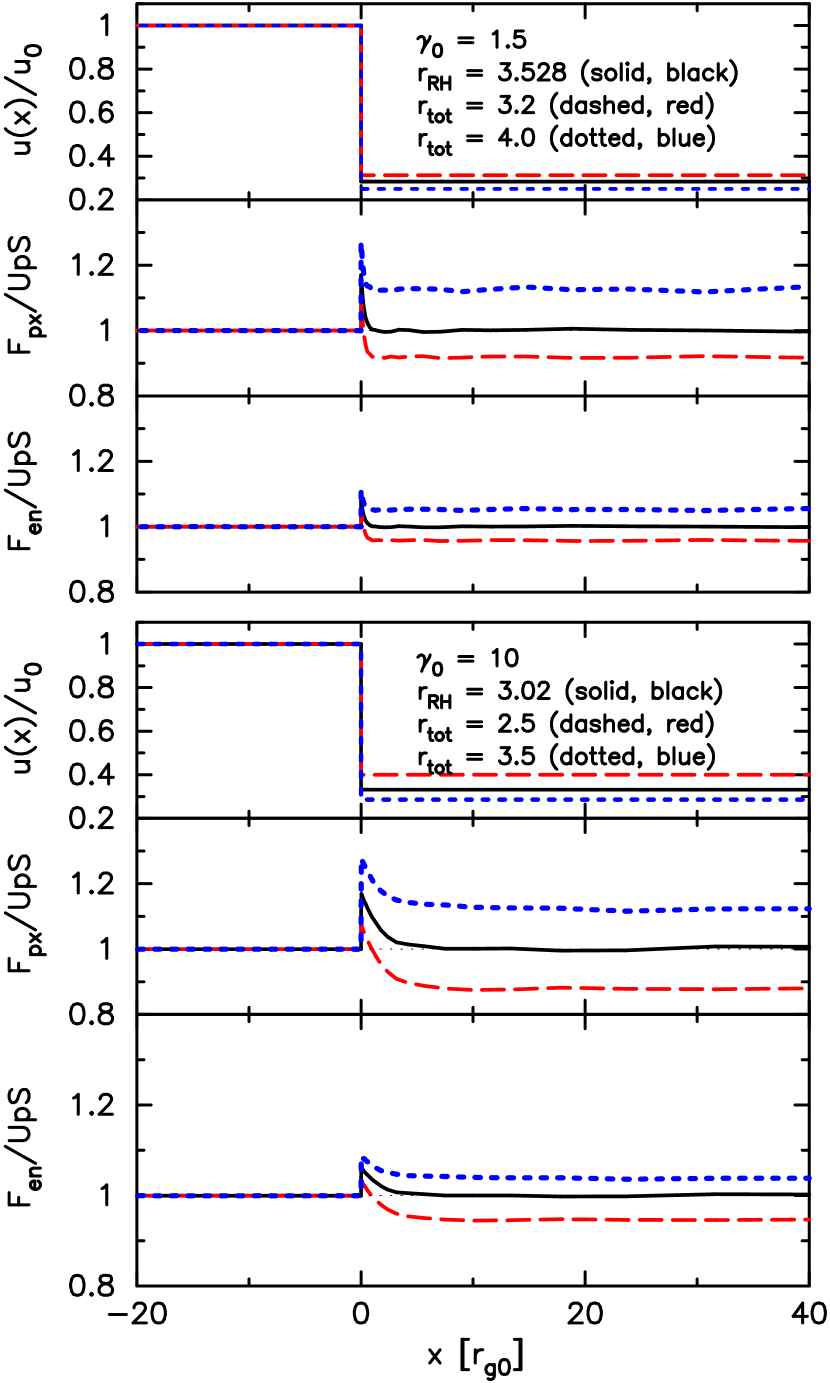
We note that the upstream energy fluxes shown in Figure 1 and elsewhere in this paper differ from those in equation (6) in that they ignore the incoming rest mass energy flux. While accelerated particles may carry away significant amounts of energy and momentum at a FEB, their density compared to the upstream plasma is always negligible, independent of almost all other factors. The rest mass energy flux entering the shock is therefore approximately equal to the rest mass energy flux leaving via downstream convection, no matter what the shock speed considered. Thus we ignore it and calculate escaping kinetic energy flux as a fraction of incoming kinetic energy flux.

Except for the region immediately downstream from the shock, the fluxes determined by the Monte Carlo simulation in Figure 1 are precisely those determined by the Rankine-Hugoniot relations for $r_{\mathrm{RH}}$, even for the trans-relativistic case $\gamma_{0}=1.5$. Results for compression ratios larger and smaller than $r_{\mathrm{RH}}$ clearly do not conserve energy and momentum. The fact that the Monte Carlo results are consistent with $r_{\mathrm{RH}}$ as determined from equations (4)–(10) is somewhat remarkable. As described in detail in Ellison & Reynolds (1991), once the basic scattering assumptions given in Section 2.1 are made, a consistent shock solution can be obtained with no further assumptions simply by running the simulation with different $r_{\mathrm{tot}}$’s. There is no need to calculate a ratio of specific heats in the Monte Carlo simulation and the fluxes are calculated directly by summing over particles as they move with the bulk flow. The fluxes shown in Figure 1 are calculated directly in the shock frame and there is no need to transform into the local frame to calculate a pressure or energy density as required in equations (4)–(10).

Of course, the reason for defining equations (4)–(7) is that, with acceleration, $r_{\mathrm{tot}}$ can be greater than $r_{\mathrm{RH}}$. This occurs because $\Gamma_{2}$ can be less than the Rankine-Hugoniot value and/or because escaping particles carry away pressure causing $r_{\mathrm{tot}}>r_{\mathrm{RH}}$ (e.g., Ellison & Eichler, 1984; Jones & Ellison, 1991; Berezhko & Ellison, 1999). Both of these nonlinear processes are included self-consistently in the Monte Carlo simulation.

2.3. Particle Injection

While background superthermal particles will be injected and accelerated if they interact with a collisionless shock, we discuss here only thermal leakage injection where all particles that get accelerated start as far upstream thermal particles.

Figure 2.— Fraction of proton number flux with shock frame momentum $p$ or greater versus $p$ for an UM shock with $\gamma_{0}=1.5$ (upper panel) and $\gamma_{0}=10$ (lower panel). Thermal particles enter the simulation far upstream from the shock and diffuse downstream. These spectra are calculated from particles that leave the shock far downstream. The values of $N_{g}$ are related to the maximum pitch-angle scattering angle by equation (3). For $N_{g}=15$, $\delta\theta_{\mathrm{max}}\simeq\pi/2$.

In our Monte Carlo technique, thermal leakage injection is modeled in its simplest form. Unshocked thermal particles, injected far upstream, convect and diffuse with a mean free path in the local frame given by equation (1). No restriction on $v_{p}/u$ is imposed. At every pitch-angle scattering event a Lorentz transformation is performed such that the particle makes an isotropic and elastic scattering in the frame of the scattering interaction. After crossing into the downstream region and interacting with the downstream plasma, some fraction of the particles will have a speed $v_{p}>u_{2}$. These particles have a certain probability to diffuse back upstream and be further accelerated. In relativistic shocks, this probability for returning back across the shock depends on the scattering parameters $N_{g}$ and $\lambda_{\mathrm{mfp}}$, and is determined stochastically for each particle in the Monte Carlo simulation.

A further assumption is that the subshock is transparent, i.e., the Monte Carlo model ignores any possible cross-shock potential or effects from enhanced magnetic turbulence, which would influence the subshock crossing probability or produce an energy change in the subshock layer. We emphasize that we do not present our injection model as a “solution” to the injection problem. Rather, it is a clearly defined process that requires no additional assumptions beyond the scattering model basic to the Monte Carlo simulation. Within statistical uncertainties, it produces unique and self-consistent shock solutions that can be compared with observations (e.g., Ellison et al., 1990b; Baring et al., 1997) or PIC simulation results (e.g., Ellison et al., 1993). Of course, the downstream return probability and the injection fraction will change substantially if an oblique magnetic field and compressed turbulence is taken into account (e.g., Niemiec et al., 2006; Lemoine & Revenu, 2006). In principle, the smooth-shock techniques we demonstrate here can be applied to this far more complicated situation.

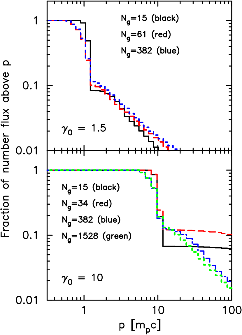
In Figure 2 we show how the injection fraction varies with $N_{g}$ for two UM shocks, one with $\gamma_{0}=1.5$ (top panel) and one with $\gamma_{0}=10$ (bottom panel). The choice of $N_{g}=15$ implies $\delta\theta_{\mathrm{max}}\simeq\pi/2$ (i.e., equation 3) and is near the extreme LAS limit. Larger values of $N_{g}$ imply fine PAS. The fraction of protons that have crossed the shock three times (up to down, down to up, and up to down again) is clearly indicated by the sharp change in the spectral shape at $p/(m_{p}c)\sim\gamma_{0}$.

For the trans-relativistic shock ($\gamma_{0}=1.5$) there is little effect from $N_{g}$, as expected, since $N_{g}$ is known to be unimportant for nonrelativistic, parallel shocks. For $\gamma_{0}=10$, $N_{g}$ does influence the injection fraction and the acceleration. For the $\gamma_{0}=10$ cases in the bottom panel of Figure 2, the smallest value of $N_{g}$ results in fewer particles injected after the first shock crossing. However the flatness of the $N_{g}=15$ and $34$ curves above $p\sim 10m_{p}c$ show that more particles continue to be accelerated for low $N_{g}$ compared to higher $N_{g}$. With a small $N_{g}$, particles move a larger distance between scattering events and will first interact with the downstream plasma further from the discontinuous shock (or subshock as the case may be) than with fine PAS. This reduces the probability that these particles will return upstream. Countering this effect, however, is the fact that when $\gamma_{0}$ is large, LAS produces larger energy gains, on average, than fine PAS for subsequent shock crossings. This can produce a harder spectrum, as seen in Figure 2 (see Ellison & Double, 2004, for a detailed discussion of this effect). While the above effect is present in the $\gamma_{0}=1.5$ plots, it is much less noticeable.

What is not shown in the UM examples in Figure 2 is that, as the shock becomes modified by the backreaction from accelerated particles, the injection fraction at the subshock automatically adjusts according to the change in the subshock compression and the pre-heating that occurs in the shock precursor.

3. Results

We now show detailed results for shock speeds spanning the range from nonrelativistic to ultra-relativistic, i.e., (A) $\beta_{0}=0.0667$ (i.e., $u_{0}=2\!\times\!10^{4}$ km s^-1); (B) $\beta_{0}=0.2$; (C) $\gamma_{0}=1.5$; (D) $\gamma_{0}=10$; and (E) $\gamma_{0}=30$.

3.1. Unmodified Shocks

In Fig. 3 we show spectra from UM shocks for nonrelativistic ($u_{0}=2\!\times\!10^{4}$ km s^-1; Model A), trans-relativistic ($\gamma_{0}=1.5$; Model C), and fully relativistic ($\gamma_{0}=10$; Model D) shock speeds. Other parameters for these shocks are given in Table 1. For the examples in Fig. 3 we have chosen $N_{g}$ large enough to obtain convergent solutions and, for each case, we plot spectra calculated at different positions relative to the subshock at $x=0$. The solid (black) curves are calculated downstream from the subshock, the dashed (red) curves are calculated upstream from the subshock at $x=-100\,r_{g0}$, and the dotted (blue) curves were calculated at the upstream FEB. The gyroradius $r_{g0}\equiv m_{p}u_{0}c/(eB_{0})$ varies with shock speed. These spectra, and all other $f(p)$ plots, are shock-frame, omni-directional, phase-space distributions.

Figure 3.— Omni-directional spectra measured in the shock frame from three unmodified shocks: $u_{0}=2\!\times\!10^{4}$ km s^-1(A), $\gamma_{0}=1.5$ (C), and $\gamma_{0}=10$ (D). All spectra are scaled to an injected flux of 1 proton-cm^-2-s^-1 and, for all models, the solid (black) spectra were calculated downstream from the shock, the dashed (red) spectra were calculated at $x=-100r_{g0}$, and the dotted (blue) spectra were calculated at the FEB. The positions of the FEB for the three shocks are: $-3\!\times\!10^{4}r_{g0}$ (A), $-10^{4}r_{g0}$ (C), and $-10^{3}r_{g0}$ (D). The thermal portions of the upstream spectra are not shown for clarity. The dashed line labeled $\sigma_{\mathrm{KW}}$ is the spectral index determined from Keshet & Waxman (2005). Note that the vertical axis is $p^{4}f(p)$.

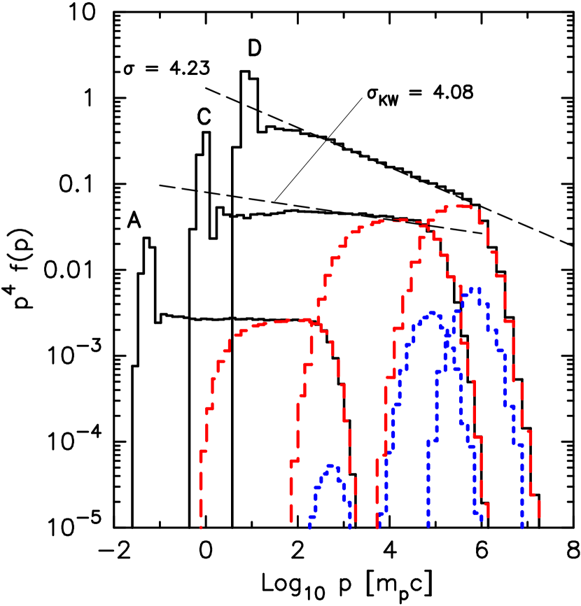
Now consider the spectra calculated downstream from the shock (black curves in Fig. 3). For the nonrelativistic shock, the particle distribution function between the thermal peak and the turnover produced by the FEB is well matched by a power law with spectral index $\sigma\simeq 4$ (i.e., $f(p)d^{3}p\propto p^{-\sigma}d^{3}p$), as expected. Also as expected, the fully relativistic case with $\gamma_{0}=10$ obtains a power law in the mid-energy range with $\sigma\simeq 4.23$, the well known ultra-relativistic result (e.g., Bednarz & Ostrowski, 1998; Kirk et al., 2000). For the trans-relativistic case ($\gamma_{0}=1.5$, $r_{\mathrm{tot}}\simeq 3.53$, Model C), we compare the Monte Carlo result against the expression from Keshet & Waxman (2005), i.e., $\sigma_{\mathrm{KW}}\simeq 4.08$ (see their equation 23) and find reasonable agreement for the power-law index in the range $p\gtrsim 300\,m_{p}c$ and below the turnover from the FEB.

The dashed and dot-dashed (red and blue) spectra calculated in the shock precursor are missing the lowest energy particles since these are not able to diffuse back upstream to the observation position. The particles that escape at the FEB (dotted, blue curves) are streaming freely away from the shock which causes the omni-directional distributions to be depressed relative to the more isotropic fluxes well within the precursor. We discuss this point with the self-consistent shock solutions shown next.

3.2. Nonlinear Relativistic Shocks

If astrophysical shocks are efficient particle accelerators the NL backreaction of the accelerated particles on the shock structure must be taken into account (e.g., Drury, 1983; Blandford & Eichler, 1987). To our knowledge, apart from PIC simulations, the only previous attempt to treat NL, relativistic shocks was the preliminary work of Ellison & Double (2002).

3.2.1 Fine scattering solutions

We now show self-consistent, fine scattering shock solutions. Again, a “fine” scattering solution has $N_{g}$ large enough so no changes, other than statistical, result if $N_{g}$ is increased.

Figure 4.— The top panels show the shock structure in terms of $u(x)/u_{0}$ (solid-black and dashed-red curves) vs. position $x$ relative to the subshock at $x=0$. Note the split log–linear scale. Length is measured in units of $r_{g0}=m_{p}u_{0}c/(eB_{0})$. The middle panels show the momentum flux $F_{\mathrm{px}}$ and the bottom panels show the energy flux $F_{\mathrm{en}}$. Values in all panels are scaled to far upstream values. In all panels, the dashed (red) curves are from an UM shock with the same input values as the modified NL shock results shown with solid (black) curves. For this nonrelativistic shock, the self-consistent compression ratio is $r_{\mathrm{NL}}=12\pm 1$ compared to the Rankine-Hugoniot value $r_{\mathrm{RH}}\simeq 3.96$. The thick horizontal dotted (blue) line in the bottom panels at $\sim 0.5$ shows the energy flux expected from our consistency conditions derived from equations (4)–(6). The FEB is at $x=-3\!\times\!10^{4}\,r_{g0}$.

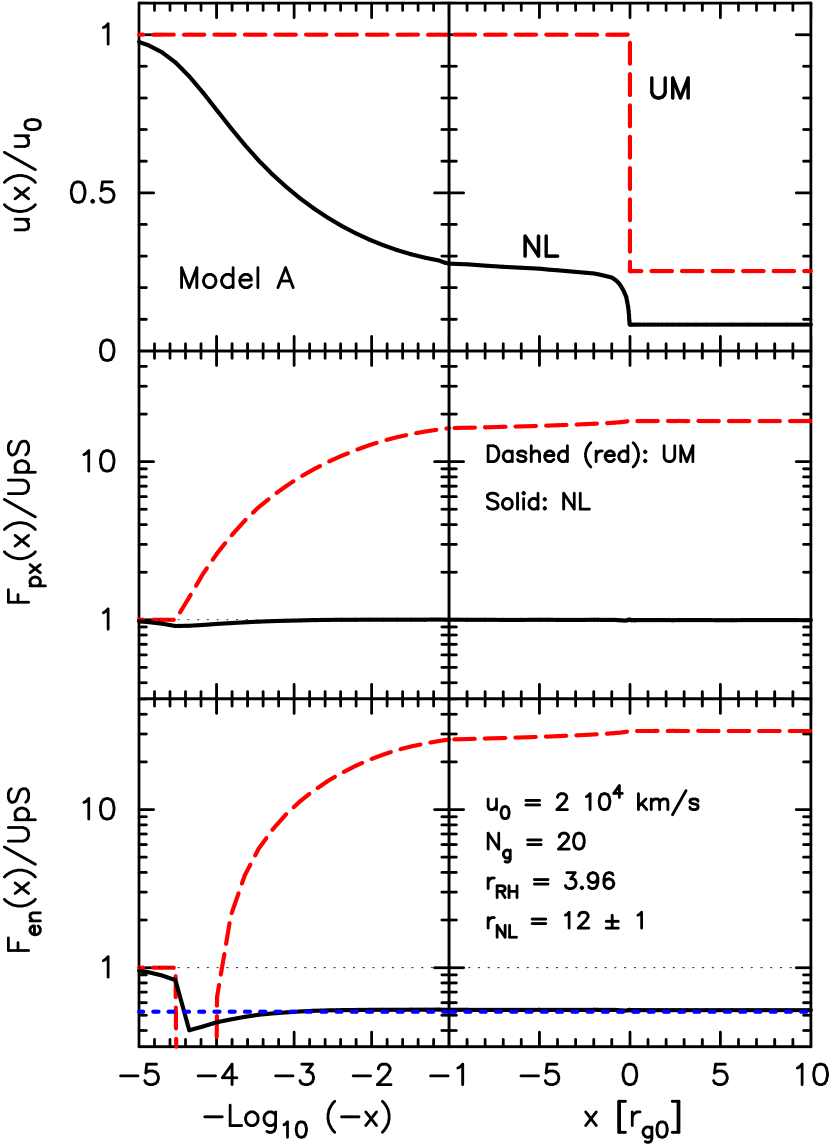
Figure 4 shows the shock structure for $u_{0}=2\!\times\!10^{4}$ km s^-1 (Model A). The dashed (red) curves show the UM solution with $r_{\mathrm{RH}}\simeq 3.96$ and it is clear from the lower panels that the momentum and energy fluxes are not conserved by large factors. Of course, the amount of acceleration depends on the injection model used, so these results are particular to the thermal leakage model contained in the Monte Carlo simulation. The solid (black) curves show the self-consistent result obtained by iteration where the shock has been smoothed and the compression ratio has been increased to $r_{\mathrm{NL}}=12\pm 1$. Now, once the escaping energy flux at the FEB is accounted for, the momentum and energy fluxes are conserved to within a few percent of the far upstream values. The heavy dotted (blue) horizontal line in the energy flux panels is the fractional energy flux (i.e., $1-Q_{\mathrm{en}}^{\mathrm{FEB}}/F_{\mathrm{en}}^{0}$), calculated from equations (4)–(6) once the modification of the downstream ratio of specific heats has been accounted for. Except for a small deviation near the FEB at $x=-3\!\times\!10^{4}\,r_{g0}$, the Monte Carlo result is consistent with equations (4)–(6). The shock structure shown in the top panels, with $r_{\mathrm{NL}}=12\pm 1$, is a consistent solution where approximately 50% of the energy flux escapes at the upstream FEB. There is essentially no escaping momentum flux as expected for a nonrelativistic shock (see Ellison, 1985).

Solutions with $r_{\mathrm{NL}}\gg r_{\mathrm{RH}}$, such as shown in Figure 4, have been known for some time for nonrelativistic shocks (e.g., Jones & Ellison, 1991; Berezhko & Ellison, 1999) and our $u_{0}=2\!\times\!10^{4}$ km s^-1 result is consistent with these previous results.

Figure 5.— Same format as Figure 4 for $\gamma_{0}=1.5$ (Model C). In all panels the dashed (red) curves show the UM case and the solid (black) curves show the self-consistent case. For this example, the expected escaping momentum and energy fluxes predicted from our consistency conditions are small, as indicated by the horizontal dotted (blue) line in the bottom panels.

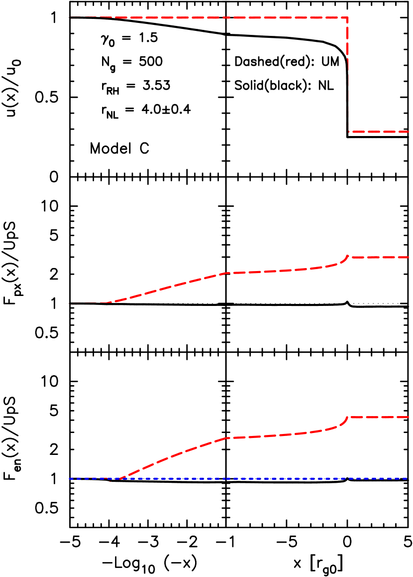
In Figure 5 we show the UM and NL shock structures for our example (C) with $\gamma_{0}=1.5$. The NL effects are present but less dramatic than for $u_{0}=2\!\times\!10^{4}$ km s^-1. For $\gamma_{0}=1.5$, the self-consistent compression ratio is $r_{\mathrm{NL}}=4.0\pm 0.4$ compared to $r_{\mathrm{RH}}\simeq 3.53$. There is an insignificant amount of escaping flux through the FEB at $x=-10^{4}\,r_{g0}$ and the momentum and energy fluxes across the shock are equal to the far upstream values to within a few percent.

For this case, the increase in $r_{\mathrm{tot}}$ comes about because the downstream ratio of specific heats, $\Gamma_{2}$, decreases from the Rankine-Hugoniot value when particles are accelerated. This decrease makes the shocked plasma more compressible and results in $r_{\mathrm{NL}}>r_{\mathrm{RH}}$. The downstream $\Gamma_{2}$ decreases from $\Gamma_{2}\simeq 1.51$, the value obtained from equation (8), to $\Gamma_{\mathrm{2,MC}}\simeq 1.47$ in the NL case, enough of a difference to explain the increased compression ratio. For the parameters we are using, $\gamma_{0}=1.5$ is a transitional speed below which strong NL effects become dominant in the fine-scattering limit.

Figure 6.— Same format as Figures 4 and 5 for $\gamma_{0}=10$ (Model D). In all panels the dashed (red) curves show the UM case and the solid (black) curves show the self-consistent case. To emphasize the shock smoothing, we show $\gamma(x)\beta(x)/(\gamma_{0}\beta_{0})$ in the top panels with a dot-dashed (blue) curve. The vertical dotted line in the top right panel shows the position of $x_{\mathrm{sub}}$.

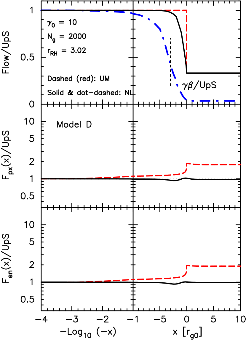
In Figure 6 we show the shock structures for our fully relativistic example (D) with $\gamma_{0}=10$. For this case, $r_{\mathrm{NL}}\simeq r_{\mathrm{RH}}\simeq 3.02$. There are no significant escaping energy or momentum fluxes at the FEB and, since the shocked particles are fully relativistic without additional acceleration, $\Gamma_{2}\simeq 4/3$. Thus, in this fine-scattering example, there are no mechanisms to increase $r_{\mathrm{tot}}$ above $r_{\mathrm{RH}}$. Nevertheless, the energy and momentum fluxes in the UM shock are nearly a factor of two above the far upstream values. A noticeable smoothing of the shock is necessary to conserve momentum and energy as shown by the $\gamma(x)\beta(x)/(\gamma_{0}\beta_{0})$ curve (dot-dashed, blue) in the top panels of Figure 6.

The smoothing parameter $x_{\mathrm{sub}}=-3\,r_{g0}$ is shown as a vertical dotted line in the top right panel of Figure 6. The flow profile to the right of this line is determined by equation (17). This is matched to the profile to the left by our algorithm based on equation (13). The procedure is iterated until consistent momentum and energy fluxes are obtained as shown by the solid (black) curves in the lower panels.

Figure 7.— Omni-directional, shock frame spectra for $u_{0}=2\!\times\!10^{4}$ km s^-1 (Model A). The curves with the thermal peaks are calculated behind the shock and the dashed (red) curves are calculated in the shock precursor at $x=-100r_{g0}$. The dotted (blue) curve is the NL spectrum calculated at the FEB. The UM spectra are the same as shown in Figure 3.

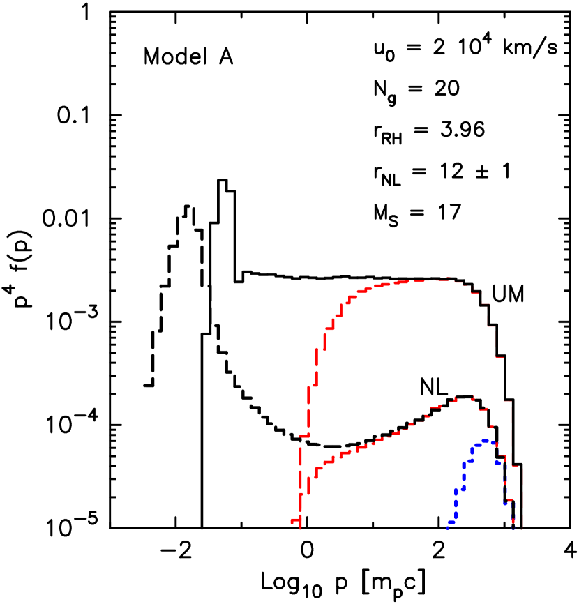
In Figure 7 we compare the UM and NL phase-space distribution functions for our $u_{0}=2\!\times\!10^{4}$ km s^-1 models. There is a dramatic difference with the superthermal NL spectra being less intense and showing the characteristic concave upward shape. The shift in the thermal peak to lower energy, which accompanies efficient DSA, is also clear in the self-consistent result. This shift is a robust prediction of DSA. When acceleration occurs, the subshock must weaken and injection must decrease to conserve energy and momentum.

We note that our nonrelativistic example has a sonic Mach number of $M_{S}\sim 17$ which is unrealistically low for such a high-speed shock in the typical interstellar medium. We have chosen parameters to yield a low $M_{S}$ for computational convenience. As shown in Berezhko & Ellison (1999), the self-consistent compression ratio is a fairly strong function of $M_{S}$ (i.e., $r_{\mathrm{tot}}\sim 1.3M_{S}^{3/4}$) when only adiabatic heating occurs in the precursor, as we assume here. Such high $r_{\mathrm{tot}}$’s make finding a self-consistent solution difficult and are almost certainly unrealistic in any case, since Alfvén wave damping is likely to be a source of heating in the precursor. The sonic Mach number becomes much less important for relativistic shocks unless the upstream temperature is high enough for the unshocked particles to have a Lorentz factor $\sim\gamma_{0}$. We do not consider such a situation here.

The distribution of escaping particles for the NL nonrelativistic shock is shown as a dotted (blue) curve in Figure 7. As shown in Figure 4, this distribution contains $\sim 50\%$ of the total energy flux but this fraction cannot be directly obtained from the omni-directional distributions we plot. (In Figure 11 below we give a direct result for the acceleration efficiency.) What Figure 7 does clearly show is that the shape of the escaping distribution is dramatically different from the downstream distribution.

Figure 8.— Comparison of UM shock spectra (Model C; same as in Figure 3) with NL shock spectra. The shock structures for these $\gamma_{0}=1.5$ shocks are shown in Figure 5. The dashed (red) curves are calculated in the shock precursor at $x=-100r_{g0}$. The dotted (blue) curve is the NL spectrum calculated at the FEB.

In Figure 8 we show the UM and NL distribution functions for our trans-relativistic example with $\gamma_{0}=1.5$. The differences between the UM and NL spectra are less than for $u_{0}=2\!\times\!10^{4}$ km s^-1 but they are still significant. The normalization of the superthermal NL distribution is approximately an order of magnitude less than the UM case and there is some slight concave curvature from the shock smoothing. While the thermal peak still shifts to a lower energy in the NL case, this shift is much less than it was for the NL nonrelativistic shock shown in Figure 7.

The escaping flux is too small to influence the shock dynamics. This is evident both from Figure 5 and from the distribution of escaping particles, shown in Figure 8 as a dotted (blue) curve. The normalization of the escaping particle distribution relative to the downstream distribution is more than an order of magnitude less than it is in the nonrelativistic case (c.f. Figure 7).

Figure 9.— Comparison of UM shock spectrum (Model D; same as in Figure 3) with NL shock spectrum. The shock structures for these $\gamma_{0}=10$ shocks are shown in Figure 6. The solid (black curves) are calculated downstream from the subshock in the shock rest frame and the dashed (red) curves are calculated in the shock precursor at $x=-100r_{g0}$.

The distribution functions for our $\gamma_{0}=10$ example (Model D) are shown in Figure 9. While the shapes of the UM and NL spectra are quite similar, they both obtain $f(p)\sim p^{-4.23}$ power laws above the thermal peak, the normalization drops by a factor of $\sim 5$ when energy and momentum conservation are taken into account. There is also a slight shift in the thermal peak to lower energy as required when DSA occurs.

Figure 10.— Nonlinear particle distributions calculated downstream from the shock in the shock rest frame for various shock speeds as indicated (Models A–E in Table 1). The spectrum for the $\gamma_{0}=1.5$ shock (dashed black curve) shows the transitional nature of nonlinear DSA. For speeds faster than $\gamma_{0}\sim 1.5$, NL effects are relatively minor. For speeds below $\gamma_{0}\sim 1.5$, strong NL effects occur and concave spectra are produced. The strong increase in normalization from $\beta_{0}=0.067$ to $\gamma_{0}=30$ mainly results from the fact that thermal particles gain more energy in their first shock crossing as the shock speed increases. The maximum momentum is determined by the position of the FEB in the various shocks.

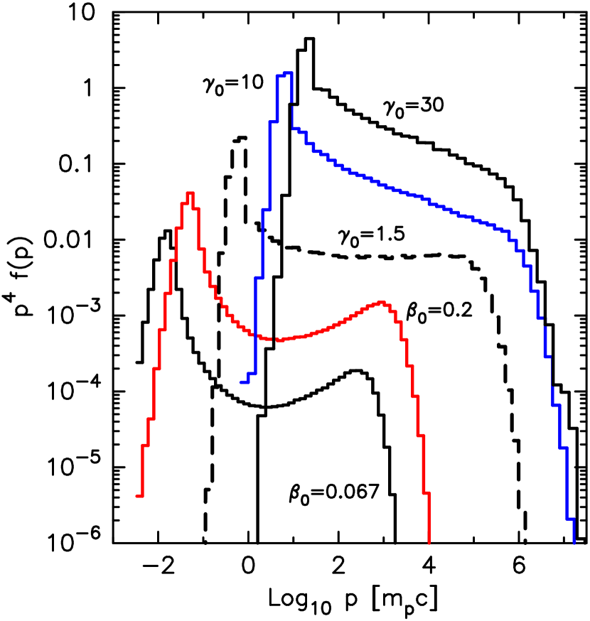
In Figure 10 we compare the self-consistent distribution functions for our five examples spanning the range from $\beta_{0}=0.067$ to $\gamma_{0}=30$. The transitional character of the spectrum at $\gamma_{0}=1.5$ is clear. At shock speeds below $\gamma_{0}\sim 1.5$, DSA can be extremely efficient and strong nonlinear effects from particle escape and $r_{\mathrm{NL}}>r_{\mathrm{RH}}$ result in concave upward spectra which are harder than $p^{-4}$ above a few GeV. These slower shocks will be strongly dependent on the input conditions, i.e., Mach number, the injection model, the position of the FEB which determines $p_{\mathrm{max}}$, assumptions concerning magnetic turbulence production and damping, and a finite speed for the magnetic scattering centers (e.g., Berezhko & Ellison, 1999; Vladimirov et al., 2008). Above $\gamma_{0}\sim 1.5$, the modified shocks have compression ratios $\sim r_{\mathrm{RH}}$ and produce spectra that are nearly $\sigma=4.23$ power laws. These faster shocks will be strongly dependent on the details of particle scattering (our parameter $N_{g}$ discussed below), and on effects from oblique geometry and compressed downstream magnetic fields which we don’t model.

Figure 11.— Acceleration efficiency in terms of the fraction of energy flux above shock frame $p$ for the $\beta_{0}=0.067$ (A), $\gamma_{0}=1.5$ (C), and $\gamma_{0}=30$ (E) shocks shown in Figure 10. These fractions include the energy flux that escapes at the upstream FEB. The escaping fraction is $\sim 0.5$ for $\beta_{0}=0.067$ but $\raise 1.29167pt\hbox{$<$\kern-7.5pt\raise-4.73611pt\hbox{$\sim$}}\,0.02$ for the two other cases.

3.2.2 Acceleration efficiency

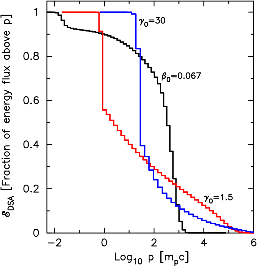
We define the acceleration efficiency, ${\cal E_{\mathrm{DSA}}}(>p)$, as the fraction of total energy flux placed in particles with shock-frame momentum $p$ or greater. This is shown in Figure 11 for three of the spectra shown in Figure 10. The other two lie between these examples. These fractions include the escaping energy flux.

If the fraction of energy above the downstream thermal peak is the measure of efficiency, all of these shocks are extremely efficient. The nonrelativistic shock ($\beta_{0}=0.067$, black curve) places over 90% of the incoming energy flux into superthermal particles. Approximately 50% of the total flux is in escaping particles. While the more relativistic shocks are less efficient, the energy flux in particles with Lorentz factors $\raise 1.29167pt\hbox{$>$\kern-7.5pt\raise-4.73611pt\hbox{$\sim$}}\,\gamma_{0}$, is still large. ${\cal E_{\mathrm{DSA}}}\sim 0.55$ for $\gamma_{0}=1.5$ and ${\cal E_{\mathrm{DSA}}}\sim 0.35$ for $\gamma_{0}=30$. For these cases, the escaping energy flux is insignificant. Additional factors, such as magnetic turbulence generation and wave damping, are not included here and will reduce the acceleration efficiency (e.g., Berezhko & Ellison, 1999; Caprioli et al., 2009).

3.2.3 Large-angle-scattering solutions

The fineness of scattering, as determined by our parameter $N_{g}$, strongly influences DSA in relativistic shocks. This effect is discussed in Ellison & Double (2004) where results for UM shocks with large-angle-scattering (LAS) (i.e., $N_{g}$ much less than the value needed for convergence) are shown. Large-angle-scattering produces hard spectra and implies efficient DSA so NL effects are certain to be important. Figure 12 (Model F) shows the dramatic effect shock smoothing has on a $\gamma_{0}=10$ shock with $N_{g}=100$ (versus $N_{g}=2000$ used to obtain the convergent $\sigma\simeq 4.23$ solution shown in Figure 6). The only difference in input parameters between this case and the shock shown in Figure 6 is $N_{g}$.

Figure 12.— Shock structure for large-angle-scattering Model F with $\gamma_{0}=10$ and $N_{g}=100$. All input parameters for this model are the same as Model D (Figure 6) except $N_{g}$. The figure format is the same as in Figure 6.

Figure 13.— Omni-directional, shock frame spectra for a $\gamma_{0}=10$ shock with large-angle-scattering, i.e., $N_{g}=100$. The solid (black) and dashed (red) curves are measured downstream from the shock and the dotted (blue) curve is the spectrum measured at the FEB for the NL shock. The peaks in the dashed (red) curve reflect discrete shock crossings in the UM shock. This coherence is removed in the smoothed NL shock.

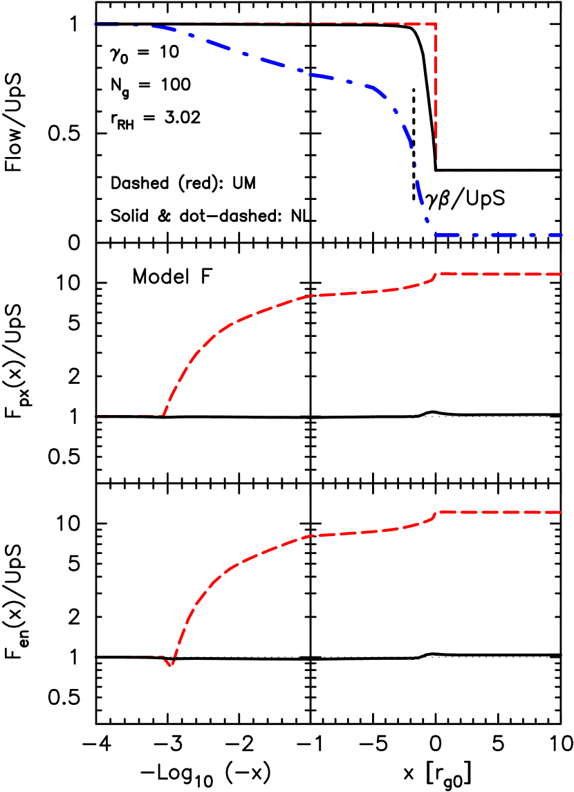
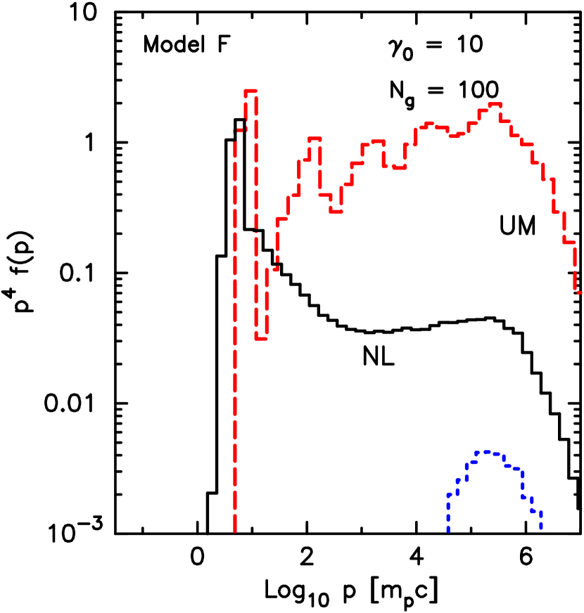
With LAS the energy flux is out of conservation by a factor of $\sim 10$ with no shock smoothing and the UM and NL particle distribution functions are vastly different as shown in the downstream spectra plotted in Figure 13. In the UM case (dashed, red curve), discrete peaks are present in $f(p)$ corresponding to a given number of shock crossings. Similar spectra were seen in Ellison, Jones, & Reynolds (1990a) and recently in Summerlin & Baring (2012). The lowest momentum peak at $p/(m_{p}c)\simeq\gamma_{0}$ is from particles that have crossed the shock once. In addition, clear peaks for three, five, and seven crossings are present, each at a momentum approximately a Lorentz factor greater then the previous peak.

The consistent NL solution is shown as the solid (black) curve in Figure 13. The peaks from discrete shock crossings seen in the UM shock are gone. The superthermal part of the spectrum is much softer, the lowest momentum peak is at a slightly lower momentum than in the UM case, and the rest of $p^{4}f(p)$ shows the concave upward curvature which is seen in efficient DSA in nonrelativistic shocks. This concave curvature is present in Fig. 9 but it is less evident because the acceleration is less efficient with $N_{g}=2000$. In Figure 13, the NL spectrum obtains a power-law index just below the turnover caused by the FEB which is slightly harder than $p^{-4}$. The NL result conserves energy and momentum and this sets the normalization of $f(p)$ which is almost a factor of 100 below the UM $f(p)$ at $p=10^{6}\,m_{p}c$.

4. Discussion

From kinematics, ultra-relativistic shocks are certain to energize incoming cold particles to $p\sim\gamma_{0}m_{0}c$ in the shock frame (see the “thermal peak” in any of our spectral plots). Diffusive shock acceleration beyond this, where particles are required to make repeated shock crossings, is much less certain.

Figure 14.— The top panel shows the shock structure for Model H matching the Summerlin & Baring (2012) example discussed in the text. The dashed (red) curve is the UM flow speed $u(x)$, the solid (black) curve is the self-consistent flow speed, and the dot-dashed (blue) curve is $\gamma(x)\beta(x)/(\gamma_{0}\beta_{0})$ for the NL shock. In the middle and bottom panels, the dashed (red) curve is the UM flux, and the solid (black) curve is the NL flux. The momentum and energy fluxes are conserved to within a few percent in the self-consistent shock.

Figure 15.— The dashed (red) curve is the downstream spectrum from the UM shock shown in Figure 14. The solid (black) curve is the NL spectrum. Note that we plot $p^{2}f(p)$ to match Figure 12 of Summerlin & Baring (2012) and the normalization of the vertical-axis is arbitrary.

4.1. Comparison with Previous Monte Carlo Results

Monte Carlo techniques have been used to study relativistic shocks for some time (e.g., Ostrowski, 1988, 1993; Ellison et al., 1990a; Bednarz & Ostrowski, 1998; Baring, 1999). Recently, using essentially the same scattering assumptions employed here, Summerlin & Baring (2012) made a comprehensive study of the plasma parameters important for test-particle DSA, including the shock obliquity. Here we compare our NL results (Model H) with the $\theta_{\mathrm{Bn}}=0^{\circ}$, $\gamma_{0}\beta_{0}=10$, $\theta_{\mathrm{scatt}}=\delta\theta_{\mathrm{max}}=\pi$ example shown in Figure 12 of Summerlin & Baring (2012) and in Figure 2 of Stecker et al. (2007). This LAS example, where $\delta\theta_{\mathrm{max}}=\pi$ implies $N_{g}\simeq 4$ from equation (2), is similar to, but more extreme than, our Model F shown in Figures 12 and 13.

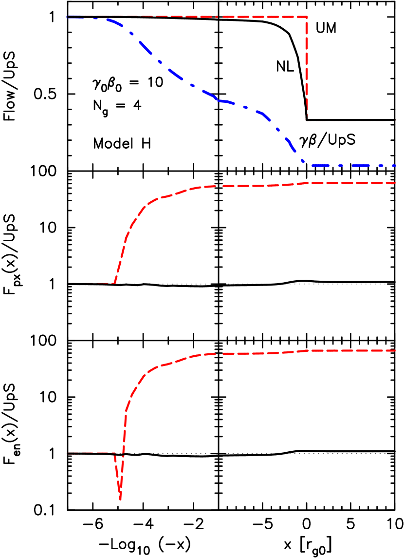
A qualitative comparison with the test-particle Summerlin & Baring (2012) result is sufficient to show the important differences that occur when a self-consistent shock structure is considered. In Figure 14 we show the shock structure and momentum and energy fluxes with (solid black curves) and without (dashed red curves) considering the backreaction of accelerated particles. The extreme LAS assumption produces very efficient acceleration in the UM shock and the momentum and energy fluxes are over-produced by nearly a factor of 100. Shock smoothing must occur unless the injection is reduced by other factors to the point where essentially only the downstream thermal distribution is present. The dot-dashed (blue) curve shows the extent of smoothing required to give a self-consistent solution.

The UM particle distribution shown in Figure 15 as a dashed (red) curve is similar to that shown in Figure 12 of Summerlin & Baring (2012). It shows the characteristic step-like structure of LAS in UM shocks. As shown by the solid black curve in Figure 15, this step-like structure disappears in the self-consistent shock. It resembles the steeper $\delta\theta_{\mathrm{max}}=\raise 1.29167pt\hbox{$<$\kern-7.5pt\raise-4.73611pt\hbox{$\sim$}}\,20^{\circ}$ examples shown in Figure 12 of Summerlin & Baring (2012). Even if turbulence is present that can result in LAS in relativistic shocks, basic conservation considerations preclude the formation of flat, step-like spectra.

In contrast to the simple scattering assumptions made here and in Summerlin & Baring (2012), the Monte Carlo studies of Niemiec, Ostrowski, & Pohl (2006), and references therein, start with a background magnetic field structure including magnetic field perturbations with various wave-power spectra in ultra-relativistic, oblique shocks. Instead of assuming pitch-angle scattering, they calculate particle trajectories directly as particles move through the background field. These test-particle results are designed to see how the background field influences the spectral shape of the accelerated population; they do not include shock smoothing or any feedback between particles and waves.

The main conclusion Niemiec, Ostrowski, & Pohl (2006) reach is that, for a wide variation of magnetic field structures, spectra are softer than the “universal” $f(p)\propto p^{-4.2}$ power law and show cutoffs at energies below the maximum resonance energy determined by the background turbulence. They call into question the ability of DSA to produce the radiating electrons seen in superluminal relativistic shock sources such as extra-galactic radio jets and GRB afterglows, or for ultra-relativistic DSA to be the mechanism to produce UHECRs (see Lemoine & Revenu, 2006, who reach somewhat different conclusions, for similar Monte Carlo work on perpendicular shocks).

Superluminal shocks require strong cross-field diffusion for DSA to occur. In an oblique shock, the de Hoffmann- Teller (H-T) frame is the frame where the $\mathrm{\bf u}\times\mathrm{\bf B}$ electric field is zero. This frame moves along the shock front at a speed $v_{\mathrm{HT}}=\gamma_{0}u_{0}\tan{\theta_{\mathrm{Bn}}}$ and shocks with $v_{\mathrm{HT}}>c$ are superluminal. A downstream particle tied to a magnetic field line cannot recross the shock and be diffusively accelerated when $v_{\mathrm{HT}}>c$. Ultra-relativistic shocks will be superluminal unless $\theta_{\mathrm{Bn}}<1/\gamma_{0}$. For $\gamma_{0}=100$, $\theta_{\mathrm{HT}}\equiv\tan^{-1}{[1/(\beta_{0}\gamma_{0})]}\simeq 0.6^{\circ}$, essentially precluding DSA in plasmas where the turbulence is too weak to produce strong cross-field diffusion. For $\gamma_{0}=1.5$, $\theta_{\mathrm{HT}}\simeq 42^{\circ}$ and far more phase space is open to DSA even without cross-field diffusion. As we have emphasized above, all of the factors that limit the efficiency of DSA in ultra-relativistic shocks, including the wave structures investigated, for example, by Niemiec, Ostrowski, & Pohl (2006), become less important as the shock slows to trans-relativistic speeds.

4.2. Comparison with PIC Results

The most compelling reason to believe that ultra-relativistic shocks do, in fact, accelerate particles beyond the initial kinematic boost comes from PIC simulations (e.g., Hoshino et al., 1992; Kato, 2007; Sironi & Spitkovsky, 2009; Keshet et al., 2009; Sironi & Spitkovsky, 2011). These simulations clearly show that acceleration occurs under some circumstances with characteristics similar to that expected from DSA. Keeping in mind the fundamental differences in how the wave-particle interactions and acceleration are treated in a PIC simulation versus a Monte Carlo simulation, we qualitatively compare our results to the $\gamma_{0}=15$, $\theta=15^{\circ}$ example shown in Sironi & Spitkovsky (2011). Here, $\theta$ is the angle between the far upstream magnetic field and the shock normal in the simulation (i.e., wall) frame of the PIC simulation. This obliquity is subluminal for $\gamma_{0}=15$, making a comparison to our parallel shock results meaningful.

Figure 16.— Nonlinear structure of a $\gamma_{0}=15$ shock with a FEB at $x=-3\,r_{g0}$ which conserves mass, momentum, and energy flux (Model F). The vertical dotted line shows the position of $x_{\mathrm{sub}}=-4\,r_{g0}$.

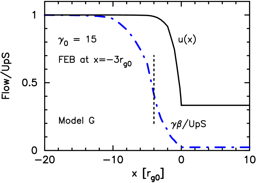
In Figure 16 we show Monte Carlo results for the structure of a NL shock with parameters chosen to produce spectra that can be compared to those in Figure 2 or 7 in Sironi & Spitkovsky (2011). In order to obtain spectra with the low cutoff energy obtained in Sironi & Spitkovsky (2011), a short shock precursor is required. We set the FEB at $x=-3\,r_{g0}$ and the dot-dashed $\gamma\beta/(\gamma_{0}\beta_{0})$ curve shows that escaping particles influence the incoming flow upstream of $x=-3\,r_{g0}$. The vertical dotted line shows the position of $x_{\mathrm{sub}}=-4\,r_{g0}$ (i.e., equation 17). For comparison, the FEB is at $x=-1000\,r_{g0}$ for our $\gamma_{0}=10$ Model D (Figures 6 and 9).

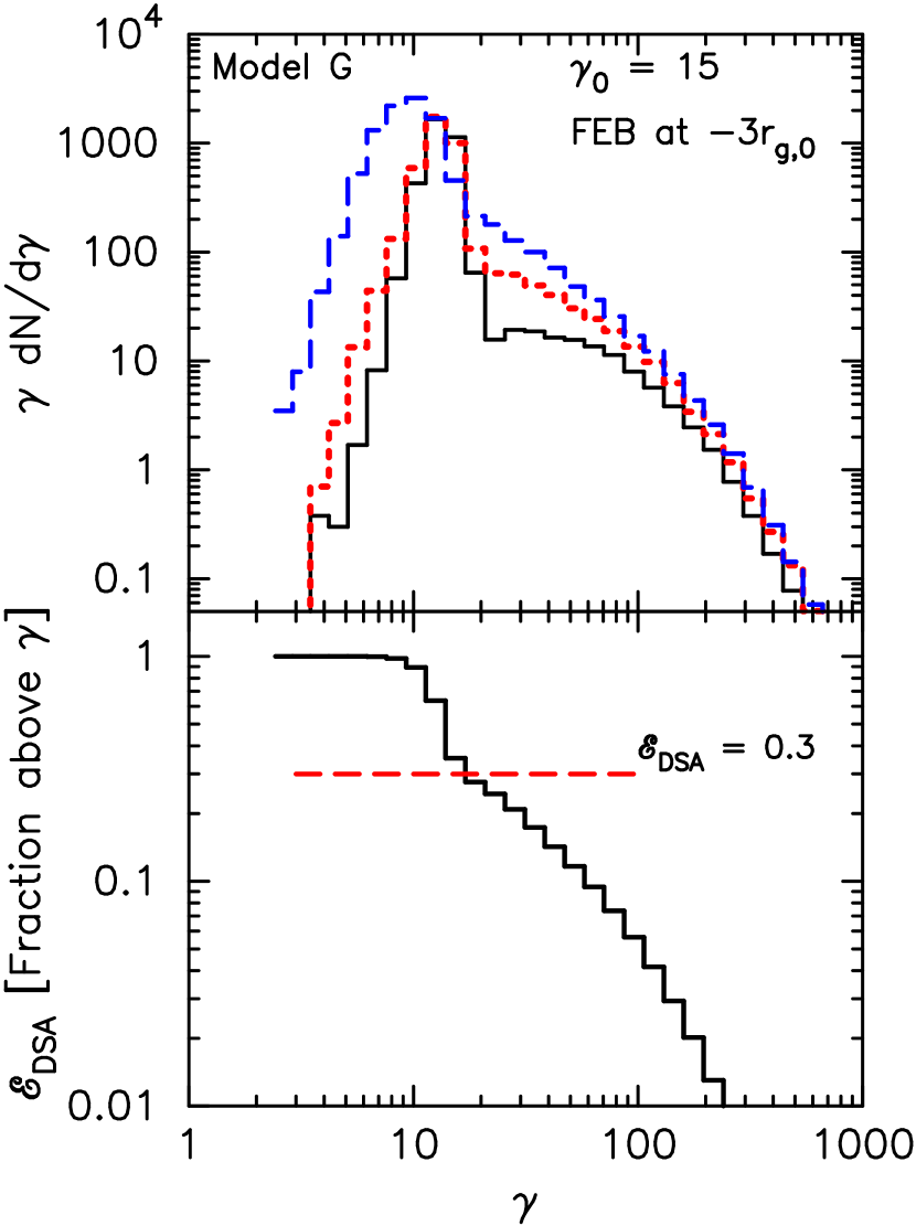
In the top panel of Figure 17 we show Monte Carlo spectra measured downstream from the subshock (dashed, blue curve) and at two upstream positions; $x=-2\,r_{g0}$ for the dotted (red) curve and $x=-2.5\,r_{g0}$ for the solid (black) curve. Considering the different nature of the simulations we have not attempted to precisely match parameters for this illustration. Nevertheless, the spectra in Figure 17, are in general qualitative agreement with the proton spectra shown in Figure 2(g), (h), and (i) of Sironi & Spitkovsky (2011).

Common features between the PIC and Monte Carlo spectra are: (i) a broad thermal peak for the downstream spectrum with much sharper thermal peaks for the upstream spectra; (ii) the downstream thermal peak is at $\gamma\simeq 10$ while the upstream peaks occur at $\gamma\simeq 15$ (if measured in the plasma frame, these upstream peaks would occur at $\sim\gamma^{2}$ here and in the PIC simulation); (iii) a relatively smooth transition from thermal to superthermal energies in the downstream spectrum as thermal particles are injected into the acceleration mechanism; (iv) a cutoff in the superthermal spectrum starting below $\gamma\sim 10^{3}$; and, (v) an acceleration efficiency (shown in the bottom panel of Figure 17 for the Monte Carlo shock) of approximately 30%.

Important differences are: (i) that the downstream Monte Carlo spectrum is softer than the PIC one and doesn’t flatten to $dN/dg\propto\gamma^{-2.1}$ before the cutoff; and, (ii) that the spectral cutoff in the Monte Carlo result is broader than the PIC cutoff and occurs for a different reason (the PIC spectrum cuts off because of a finite run time, while the Monte Carlo spectrum cuts off because we have imposed a FEB at $x=-3r_{g0}$ to produce a cutoff at an energy similar to that obtained in the PIC result).

Figure 17.— The top panel shows the omni-directional, shock frame spectra for a NL $\gamma_{0}=15$ shock with a FEB at $x=-3\,r_{g0}$ (Model G). The solid (black) curve is measured at $x=-2.5\,r_{g0}$, the dotted (red) curve is measured at $x=-2\,r_{g0}$, and the dashed (blue) curve is measured downstream from the subshock at $x=5\,r_{g0}$. The bottom panel shows the acceleration efficiency and the horizontal dashed line marks the efficiency found by Sironi & Spitkovsky (2011) using a PIC simulation for a shock with similar parameters.

Shock modification by the backpressure of accelerated particles is also clearly present in both cases, as seen in our Figure 16 and the top panel of Figure 4 in Sironi & Spitkovsky (2011). Of course, the scaling of the shock structure, which depends on the magnetic field, is quite different. The self-consistent field in the PIC result is highly turbulent, time-dependent, and varies strongly with location. It also includes magnetic field amplification, presumably by Bell’s instability (e.g., Bell, 2004, 2005). In the Monte Carlo simulation Bohm diffusion is assumed and the field is uniform and set to $B_{0}=3$ $\mu$G. Nevertheless, shock modification must occur to satisfy energy and momentum conservation and the fact that the PIC and Monte Carlo shocks have similar acceleration efficiencies means the gross features of the shock structure will be similar.

Shock reformation is another notable aspect of the PIC results that is not modeled by our steady-state Monte Carlo simulation. In the time-dependent PIC simulations, bunches of downstream ions can return back upstream causing the subshock to disrupt and reform in a quasi-periodic fashion. While this process might be important for determining local particle reflection and other injection effects, the relatively narrow temporal and spatial averages applied by Sironi & Spitkovsky (2011) in their Figures 4 and 7 for example seem to smooth the density profiles and energy spectra enough so long-term effects from reformation are no longer evident. This suggests that our steady-state Monte Carlo results can be meaningfully compared to averages taken during the evolving PIC simulations.

4.3. GRB Afterglows

The radiation observed from GRB afterglows is generally modeled as synchrotron  emission from relativistic electrons, where the electrons are accelerated by the ultra-relativistic but decelerating fireball shock. A further assumption that is generally made is that the electrons obtain a power-law distribution with some minimum Lorentz factor that emerges from DSA (e.g., Mészáros, 2002; Piran, 2004; Leventis et al., 2013). Equally constraining, the shape of the electron distribution is often assumed to remain constant during the evolution of the blastwave as it slows in the circumstellar medium (CSM). As the PIC and Monte Carlo results we have discussed show, ultra-relativistic shock theory has difficulty supporting these widely used assumptions.

The ejecta moving relativistically from the central engine in a GRB will drive a forward shock (FS) into the circumstellar material (CSM) and a reverse shock (RS) will propagate through the ejecta material (e.g., Piran, 2004, and references therein). Initially, the FS will be ultra-relativistic but the RS may initially be nonrelativistic.

In the case of matter dominated ejecta with a density $\Delta$ times the density of the CSM, the Lorentz factor of the RS, $\gamma_{\mathrm{RS}}$, in the rest frame of the ejecta, can be estimated as:

$$\gamma_{\mathrm{RS}}\approx\left\{\begin{array}[]{ll}1+\frac{4}{7}\gamma_{\mathrm{ej}}^{2}\Delta^{-1},&\gamma_{\mathrm{ej}}^{2}\ll\Delta\\ \frac{1}{\sqrt{2}}\gamma_{\mathrm{ej}}^{1/2}\Delta^{-1/4},&\gamma_{\mathrm{ej}}^{2}\gg\Delta\,,\end{array}\right.$$ (18)

where $\gamma_{\mathrm{ej}}$ is the Lorentz factor of the ejecta (see Piran, 2004). In the early expansion stage, when the ejecta density is large and $\gamma_{\mathrm{ej}}^{2}\ll\Delta$, the reverse shock is nonrelativistic. It will become mildly relativistic when $\gamma_{\mathrm{ej}}^{2}\sim\Delta$. While the energy in the RS is much less than in the ultra-relativistic FS, we have shown (e.g., Figure 10) that DSA is more efficient in trans-relativistic shocks and the spectrum produced is harder than for ultra-relativistic shocks.

In the case of GRBs driven by ejecta that is initially magnetically dominated (e.g., Lyutikov & Blandford, 2003; Zhang & Yan, 2011), a trans-relativistic RS may form during the afterglow stage if efficient magnetic dissipation occurs during the prompt emission regime (e.g., Zhang & Yan, 2011; Bykov & Treumann, 2011; Bykov et al., 2012).

Figure 18.— Structure for a $\gamma_{0}=1.5$ shock with a FEB at $-10^{8}\,r_{g0}$ (Model I). The figure format is the same as Figure 5. The self-consistent compression ratio is $r_{\mathrm{NL}}=4.0\pm 0.4$ compared to the Rankine-Hugoniot value $r_{\mathrm{RH}}\simeq 3.53$.

The main reason for considering a trans-relativistic RS, rather than the ultra-relativistic FS, that carries far more energy, as the source of the afterglow, are the conceptual difficulties superluminal ultra-relativistic shocks have in diffusively injecting and accelerating particles to energies needed to model GRB afterglows (e.g., Pelletier, Lemoine, & Marcowith, 2009). Whatever difficulties ultra-relativistic shocks have should be less for trans-relativistic shocks. Furthermore, our parallel-shock approximation is more applicable to subluminal trans-relativistic shocks.

4.4. Trans-relativistic Supernovae and UHECRs

Recently, mildly relativistic type Ibc supernovae have been discovered (e.g., Soderberg et al., 2010; Paragi et al., 2010; Chakraborti et al., 2011) with inferred blast-wave speeds such that $\gamma_{0}\beta_{0}\sim 1$. These speeds lie between normal supernova remnants (SNRs) with $10^{-3}\raise 1.29167pt\hbox{$<$\kern-7.5pt\raise-4.73611pt\hbox{$\sim$}}\,\gamma_{0}\beta_{0}\raise 1.29167pt\hbox{$<$\kern-7.5pt\raise-4.73611pt\hbox{$\sim$}}\,\,0.1$ and GRB jets or fireballs with $\gamma_{0}\beta_{0}\raise 1.29167pt\hbox{$>$\kern-7.5pt\raise-4.73611pt\hbox{$\sim$}}\,5$ and suggest there may be a continuum of shock speeds from the explosions of massive stars over the full range from nonrelativistic to ultra-relativistic (see, for example, Lazzati et al., 2012).

Figure 19.— Comparison of UM downstream spectrum (dashed, red curve) for our Model I with $L_{\mathrm{FEB}}=-10^{8}\,r_{g0}$ against the NL spectrum (solid, black curve).

Our trans-relativistic results are important for the interpretation of emission from shock accelerated particles in this particular class of mildly relativistic type Ibc SNe. We showed in Figure 8 that phase-space spectra $f(p)\propto p^{-4}$ can be expected in a transitional zone around $\gamma_{0}\sim 1.5$ ($\gamma_{0}\beta_{0}\sim 1$). Perhaps more importantly however, all relativistic blast-wave shocks will slow as they sweep up material and, if DSA is working as modeled in Figure 10, relativistic shocks will surely pass through a transitional phase.

Budnik et al. (2008) have suggested that galactic trans-relativistic SNe may produce cosmic rays (CRs) with energies in the range $\sim 10^{15}$ to $\sim 10^{18}$ eV. An even more dramatic assertion by Chakraborti et al. (2011) is that the sub-population of type Ibc SNe such as SN 2009bb may be able to produce UHECRs to the Greisen-Zatsepin-Kuzmin (GZK) limit.

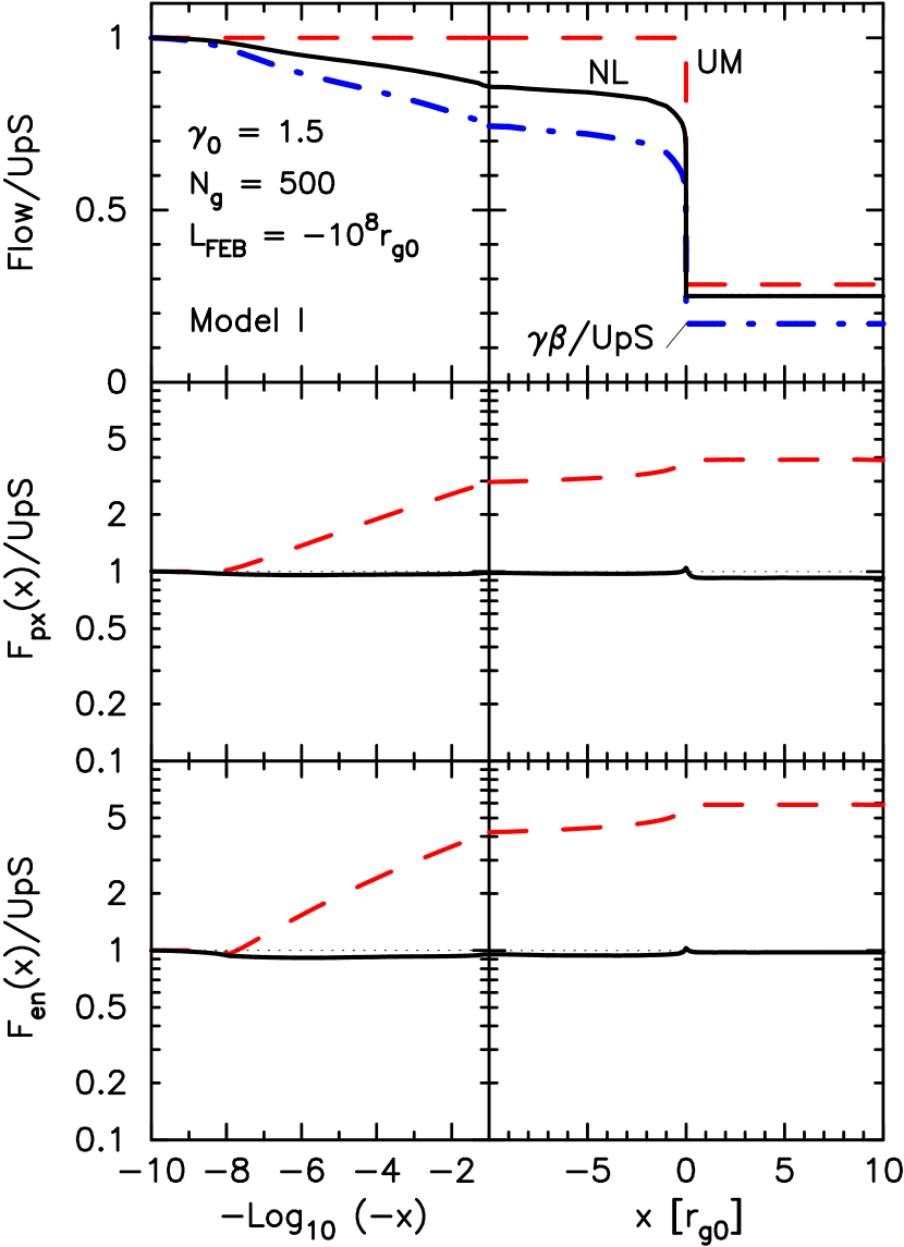
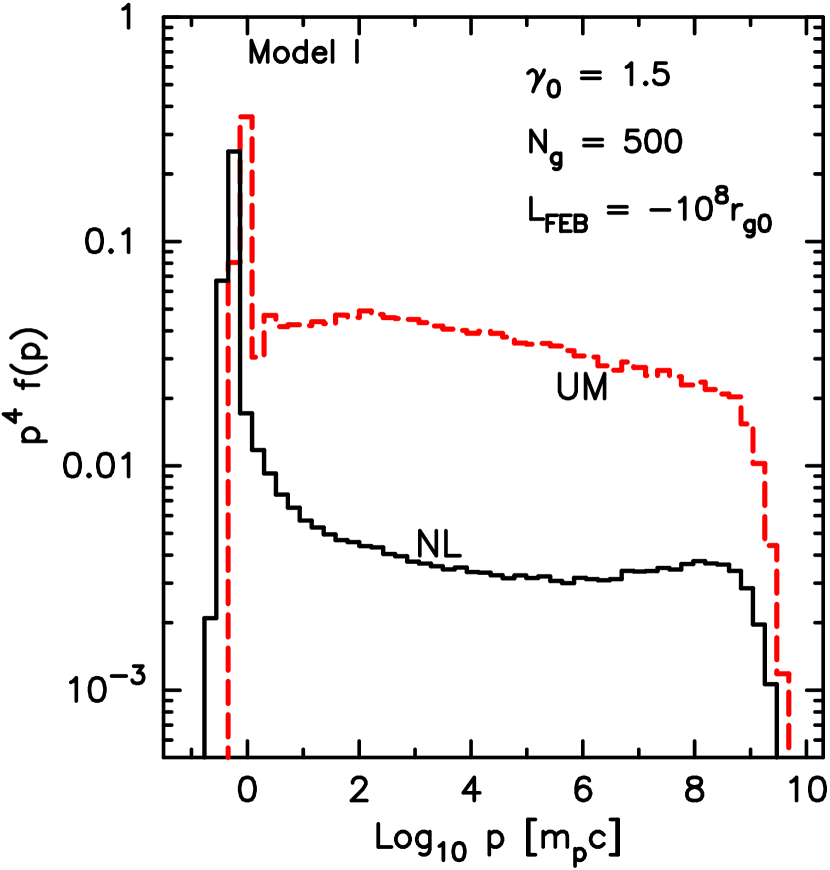
In our steady-state simulation, for a given set of shock parameters including $\eta_{\mathrm{mfp}}$ and $N_{g}$, the maximum energy a shock can produce, $E_{\mathrm{max}}$, is proportional to the distance to the FEB, $L_{\mathrm{FEB}}$. Of course, in our plane-shock model, the FEB mimics the effects of a finite shock where $L_{\mathrm{FEB}}$ corresponds to the scale set by the shock radius or system size, an approximation that has been used to good effect in models of young nonrelativistic SNRs (e.g., Lee et al., 2013). In Figures 18 and 19 (Model I), we show results for a $\gamma_{0}=1.5$ shock where $L_{\mathrm{FEB}}=-10^{8}r_{g0}\sim 0.25$ pc and $B_{0}=300$ $\mu$G. All other parameters are the same as those used for Model C shown in Figures 5 and 8. $L_{\mathrm{FEB}}$ and $B_{0}$ have been chosen to obtain $E_{\mathrm{max}}\sim 10^{18}$ eV before the turnover from CRs escaping at the FEB. The large $B_{0}$ assumes that this $\gamma_{0}=1.5$ shock can produce strong magnetic field amplification or that it exists in a region with large ambient fields. While the evidence supporting strong MFA in nonrelativistic shocks is convincing (e.g., Cassam-Chenaï et al., 2007), little MFA is expected in ultra-relativistic shocks. However, since MFA is driven by CR production, we expect the spectral transition seen in Figure 10 to be accompanied by MFA as the efficiency of DSA increases and the shock speed slows.

As indicated by the dot-dashed (blue) curve in the top panels of Figure 18, the shock precursor is noticeably smoothed over the entire region from $L_{\mathrm{FEB}}$ to the subshock. In Figure 19, the concave shape of the NL spectrum (solid, black curve) is obvious but, to a fair approximation, the spectrum is harder than the UM one and $f(p)\propto p^{-4}$ over a wide momentum range. Of course, we have made the assumption that Bohm diffusion, with $B_{0}\sim 300$ $\mu$G, occurs over the scale indicated in Figure 18 (e.g., Milosavljević & Nakar, 2006). If this in fact happens, trans-relativistic shocks might be able to produce CRs to $\sim 10^{18}$ eV.

Another possible source of UHECRs involving DSA in trans-relativistic shocks are jets in active galactic nuclei (AGN) (see, for example, Kotera & Olinto, 2011; Aharonian et al., 2012, for reviews). Shock speeds of $\beta_{0}\sim 0.3$ have been inferred from multi-waveband observations in a number of radio hot spots (e.g., Meisenheimer et al., 1989) and Romero et al. (1996) suggest that the trans-relativistic jet in Centaurus A (NGC 5128), the closest AGN, may accelerate CRs to $E_{\mathrm{max}}>10^{21}$ eV. For this $E_{\mathrm{max}}$, a shock size of $\sim 2$ kpc and a field of $\sim 10$ $\mu$G were assumed. Lemoine & Waxman (2009) established that a jet magnetic luminosity of $L_{B}\gtrsim 10^{45}Z^{-2}$ erg s^-1 is needed in order to accelerate particles of charge number $Z$ up to 100 EeV. Since $L_{B}$ for Centaurus A is estimated to be $\raise 1.29167pt\hbox{$>$\kern-7.5pt\raise-4.73611pt\hbox{$\sim$}}\,10^{43}$ erg s^-1, the production of CRs to $\sim 10^{21}$ eV may be possible.

5. Conclusions

If collisionless shocks accelerate particles efficiently the shock structure must be calculated self-consistently with the acceleration and particle escape to conserve energy and momentum. We have presented a Monte Carlo model of nonlinear DSA that, once the scattering properties are defined, determines the thermal injection and shock structure in plane-parallel, steady-state shocks of arbitrary Lorentz factor. Our injection model, parameterized diffusion, and plane-parallel, steady-state approximations are restrictive when compared to PIC simulations and some Monte Carlo calculations that trace particle orbits. However, apart from PIC simulations and the preliminary work of Ellison & Double (2002), they are the first to model DSA in NL relativistic shocks. Nonlinear effects may be critical for understanding GRB afterglows, blazars (e.g., Stecker et al., 2007), radio jets (e.g., Wykes et al., 2013), and DSA in a newly discovered class of mildly relativistic type Ibc SNe (e.g., Budnik et al., 2008; Soderberg et al., 2010). Next is a list of our major findings.

(i) In terms of the backreaction of CRs on the shock structure, NL DSA works identically in nonrelativistic and relativistic shocks, since the effects we consider depend only on energy and momentum conservation. Quantitative differences result from the fact that relativistic shocks tend to have a lower intrinsic compression ratio than nonrelativistic shocks and because particle distributions are highly anisotropic in relativistic shocks. Besides making the analysis of NL DSA more difficult, this anisotropy makes relativistic shocks much more sensitive to assumptions made regarding particle diffusion and, unlike in nonrelativistic shocks, these assumptions can strongly influence the acceleration process. We do not specify the production mechanism of self-generated magnetic turbulence here but rather assume that Bohm diffusion applies. There are fundamental problems in how, or even if, this turbulence is created that depend on shock speed and obliquity (see, for example, Plotnikov et al., 2013, and references therein).

(ii) There is a smooth transition between the concave upward spectral shape long established for nonrelativistic shocks undergoing efficient DSA and the soft power-law spectrum predicted for fully relativistic shocks (i.e., Figure 10). For the parameters used here, this transition occurs around $\gamma_{0}=1.5$, a speed recently associated with a subclass of type Ibc SNe (e.g., Soderberg et al., 2010). An increase in MFA can also be expected as shocks slow and cross this transition zone.

(iii) Even though NL effects from particle acceleration are weaker in fully relativistic shocks than in nonrelativistic ones, they nevertheless have a substantial effect on the accelerated particle spectrum. Our NL results for $\gamma_{0}=10$, in the fine scattering limit, show the normalization of the energetic particle distribution dropping by a factor of about 5 compared to the UM shock (see Figure 9). While these specific results depend quantitatively on the details of our model, basic energy and momentum conservation demands similar backreaction effects if DSA is efficient.

(iv) If large-angle-scattering is assumed in relativistic shocks, particles can gain a much larger amount of energy in a given shock crossing than for fine pitch-angle scattering. While this suggests that these shocks can be extremely efficient accelerators with hard spectra, NL shock smoothing reduces the resultant efficiency and softens the spectrum considerably (see Figures 13 and 15).

(v) Not forgetting the fundamental differences between our Monte Carlo technique and PIC simulations, we have compared our results with those of Sironi & Spitkovsky (2011) and shown that important similarities exist in the spectral shape, average shock structure, and overall acceleration efficiency determined by each technique for a quasi-parallel, subluminal shock (see Figures 16 and 17). Our results also suggest that short time-scale shock reformation effects can be adequately modeled with a steady-state simulation.

(vi) The major reason for employing the Monte Carlo technique, when far more physically complete PIC simulations exist, is indicated by Figures 18 and 19. It has been suggested that trans-relativistic shocks may be able to produce CRs to $10^{18}$ eV and above. In order to model such acceleration, large spatial and time scales are required which remain well beyond PIC limits. To obtain $E_{\mathrm{max}}\sim 10^{18}$ eV, we needed $L_{\mathrm{FEB}}=-10^{8}\,r_{g0}$ for our $\gamma_{0}=1.5$ shock, compared to $L_{\mathrm{FEB}}=-3\,r_{g0}$ used for our $\gamma_{0}=15$ comparison to the Sironi & Spitkovsky (2011) results (Model G). After adjusting for the different magnetic fields and shock speeds used in our length unit $r_{g0}$, this is a factor of $\sim 2.5\!\times\!10^{5}$ difference in real units, a factor easily accommodated by the Monte Carlo technique.

The most important approximations made by the Monte Carlo technique are:
(i) The particle scattering is parameterized using $\eta_{\mathrm{mfp}}$ (equation 1) and $N_{g}$ (equation 3). For this study, we only show results for Bohm diffusion, i.e., $\eta_{\mathrm{mfp}}=1$, although our plane-parallel results are independent of $\eta_{\mathrm{mfp}}$ if the one length scale in the problem, the FEB, is scaled in particle gyroradii. Our scattering parameterization has no spatial dependence and does not include magnetic field amplification, a process almost certain to be important in strong, nonrelativistic shocks (e.g., Bell, 2004; Vladimirov et al., 2008; Ellison et al., 2012), and one that has been invoked to explain UHECR production in trans-relativistic shocks (e.g., Chakraborti et al., 2011). We note that the high acceleration efficiencies we find, and the related concave spectral shapes, may be less extreme in oblique shocks where values of $\eta_{\mathrm{mfp}}>1$. Difficulties in producing strong turbulence in ultra-relativistic, superluminal shocks may also result in larger effective $\eta_{\mathrm{mfp}}$’s, reducing NL effects from DSA and resulting in lower cutoff energies in any given shock environment. In the critical trans-relativistic, subluminal regime, however, effects from shock obliquity are less restrictive and strong turbulence is more likely to be produced, making our Bohm diffusion approximation more plausible.

(ii) The damping of magnetic turbulence isn’t included. The strong NL effects we see will be lessened if the shock precursor is heated as energy is transferred from the turbulence to the background plasma.

(iii) We only model plane, parallel shocks while relativistic shocks are expected to be oblique. Based on PIC simulation results (e.g., Sironi & Spitkovsky, 2011), the consequences of this restriction should be minor as long as the shock remains subluminal. However, important relativistic shock applications, such as the termination shock in a pulsar wind nebula, are likely to be strongly superluminal. While oblique, relativistic, test-particle shocks have been studied with Monte Carlo techniques (e.g., Ellison & Double, 2004; Summerlin & Baring, 2012), NL effects have not yet been modeled.

(iv) We have only modeled protons while applications involving radiation signatures of relativistic shocks require electrons to be accelerated self-consistently with protons. Electrons can be included in the Monte Carlo model (e.g., Baring et al., 1999) but, unlike self-consistent PIC results, this requires additional assumptions and free parameters. Electrons will be considered in future work.

(v) Our Monte Carlo model is steady-state while most astrophysical shocks are in evolving systems. However, as suggested by Figure 10, an evolving system can be approximated with several steady-state shocks, each differing in parameters such as radius, speed, ambient density, and magnetic field strength.

Diffusive shock acceleration is the most intensively investigated acceleration mechanism in astrophysics for good reason. Collisionless shocks are common, some nonrelativistic shocks are known from in situ spacecraft observations to be efficient accelerators with self-generated magnetic turbulence, and detailed predictions from nonrelativistic DSA theory provide excellent fits to some nonthermal sources (see Lee, Mewaldt, & Giacalone, 2012, for a review). From its introduction in 1976-78, the theory of DSA developed rapidly, benefiting from the combined input from direct spacecraft observations of heliospheric shocks, analytic studies, and computer simulations. The extension of DSA theory to ultra-relativistic shocks is a natural progression but definitive results have been slowed by the inherent difficulty associated with magnetic turbulence generation and particle transport in relativistic plasmas, and by the fact that no relativistic shocks are directly observable by spacecraft.

What is certain is that there must be a smooth transition between efficient, nonrelativistic shocks, where observational evidence suggests that DSA produces strong MFA in the shock precursor, and ultra-relativistic shocks, which may be far less efficient accelerators and where self-generated turbulence may be weak or absent. The Monte Carlo model we present here provides important information on the critical trans-relativistic regime, albeit for a simple parameterized scattering model. More physically motivated diffusion has been included in nonrelativistic versions of the code (e.g., Vladimirov et al., 2008, 2009) and, in principle, similar generalizations can be made to the relativistic code.

Table 1Shock parameters.

Model	[$u_{0}$] {$\beta_{0}$} $\gamma_{0}$	$N_{g}$	$M_{S}$	$r_{\mathrm{RH}}$	$r_{\mathrm{NL}}$	$|x_{\mathrm{sub}}|$	$|L_{\mathrm{FEB}}|$	$L_{\mathrm{FEB}}$	${\cal E_{\mathrm{DSA}}}$	$q_{\mathrm{en}}^{\mathrm{FEB}}$
	[km s-1]					$r_{g0}$	$r_{g0}$	[pc]
A	[$2\!\times\!10^{4}$]	20	17	3.96	$12\pm 1$	0	$3\!\times\!10^{4}$	$6\!\times\!10^{-4}$	$0.93$	$0.5$
B	{0.2}	60	16	3.93	$11\pm 1$	0	$1\!\times\!10^{4}$	$7\!\times\!10^{-4}$	$0.9$	$0.45$
C	1.5	500	$1900$	3.53	$4.0\pm 0.4$	0	$1\!\times\!10^{4}$	$2.5\!\times\!10^{-3}$	$0.55$	$0.02$
D	10	2000	$2\!\times\!10^{3}$	3.02	3.02	$3$	$1000$	$3.4\!\times\!10^{-4}$	$0.3$	$<0.01$
E	30	$10^{4}$	$2\!\times\!10^{3}$	3.00	3.00	$9$	$100$	$3.4\!\times\!10^{-5}$	$0.35$	$<0.01$
F	10	$100$	$2\!\times\!10^{3}$	3.02	3.02	$1.75$	$1000$	$3.4\!\times\!10^{-4}$	$0.5$	$0.01$
G	15	2000	8	3.00	3.00	4	3	$1\!\times\!10^{-6}$	0.3	$<0.1$
H	10.05	4	1800	3.02	3.02	3.2	$1\!\times\!10^{5}$	$3.4\!\times\!10^{-2}$	0.8	$<0.1$
I	1.5	500	1900	3.53	$4.0\pm 0.4$	0	$1\!\times\!10^{8}$	0.25	0.6	0.01

References

- Aharonian et al. (2012) Aharonian, F., Bykov, A., Parizot, E., Ptuskin, V., & Watson, A. 2012, Space Sci. Rev., 166, 97
- Axford et al. (1977) Axford, W. I., Leer, E., & Skadron, G. 1977, Proc. 15th ICRC(Plovdiv), 11, 132
- Baring (1999) Baring, M. 1999, in International Cosmic Ray Conference, Vol. 4, International Cosmic Ray Conference, 5
- Baring (2004) Baring, M. G. 2004, Nuclear Physics B Proceedings Supplements, 136, 198
- Baring et al. (1999) Baring, M. G., Ellison, D. C., Reynolds, S. P., Grenier, I. A., & Goret, P. 1999, ApJ, 513, 311
- Baring et al. (1997) Baring, M. G., Ogilvie, K. W., Ellison, D. C., & Forsyth, R. J. 1997, ApJ, 476, 889
- Bednarz & Ostrowski (1998) Bednarz, J. & Ostrowski, M. 1998, Physical Review Letters, 80, 3911
- Bell (1978) Bell, A. R. 1978, MNRAS, 182, 147
- Bell (2004) Bell, A. R. 2004, MNRAS, 353, 550
- Bell (2005) Bell, A. R. 2005, MNRAS, 358, 181
- Berezhko & Ellison (1999) Berezhko, E. G. & Ellison, D. C. 1999, ApJ, 526, 385
- Blandford & Eichler (1987) Blandford, R. & Eichler, D. 1987, Physics Reports, 154, 1
- Blandford & Ostriker (1978) Blandford, R. D. & Ostriker, J. P. 1978, ApJ, 221, L29
- Blasi & Vietri (2005) Blasi, P. & Vietri, M. 2005, ApJ, 626, 877
- Budnik et al. (2008) Budnik, R., Katz, B., MacFadyen, A., & Waxman, E. 2008, ApJ, 673, 928
- Bykov et al. (2012) Bykov, A., Gehrels, N., Krawczynski, H., et al. 2012, Space Sci. Rev., 173, 309
- Bykov & Treumann (2011) Bykov, A. M. & Treumann, R. A. 2011, A&A Rev., 19, 42
- Caprioli et al. (2009) Caprioli, D., Blasi, P., Amato, E., & Vietri, M. 2009, MNRAS, 395, 895
- Cassam-Chenaï et al. (2007) Cassam-Chenaï, G., Hughes, J. P., Ballet, J., & Decourchelle, A. 2007, ApJ, 665, 315
- Chakraborti et al. (2011) Chakraborti, S., Ray, A., Soderberg, A. M., Loeb, A., & Chandra, P. 2011, Nature Communications, 2
- Double et al. (2004) Double, G. P., Baring, M. G., Jones, F. C., & Ellison, D. C. 2004, ApJ, 600, 485
- Drury (1983) Drury, L. O. 1983, Reports of Progress in Physics, 46, 973
- Ellison (1985) Ellison, D. C. 1985, J. Geophys. Res., 90, 29
- Ellison et al. (1996) Ellison, D. C., Baring, M. G., & Jones, F. C. 1996, ApJ, 473, 1029
- Ellison & Double (2002) Ellison, D. C. & Double, G. P. 2002, Astroparticle Physics, 18, 213
- Ellison & Double (2004) Ellison, D. C. & Double, G. P. 2004, Astroparticle Physics, 22, 323
- Ellison & Eichler (1984) Ellison, D. C. & Eichler, D. 1984, ApJ, 286, 691
- Ellison et al. (1993) Ellison, D. C., Giacalone, J., Burgess, D., & Schwartz, S. J. 1993, J. Geophys. Res., 98, 21085
- Ellison et al. (1990a) Ellison, D. C., Jones, F. C., & Reynolds, S. P. 1990a, ApJ, 360, 702
- Ellison et al. (1990b) Ellison, D. C., Moebius, E., & Paschmann, G. 1990b, ApJ, 352, 376
- Ellison & Reynolds (1991) Ellison, D. C. & Reynolds, S. P. 1991, ApJ, 378, 214
- Ellison et al. (2012) Ellison, D. C., Slane, P., Patnaude, D. J., & Bykov, A. M. 2012, ApJ, 744, 39
- Giacalone & Ellison (2000) Giacalone, J. & Ellison, D. C. 2000, J. Geophys. Res., 105, 12541
- Hoshino et al. (1992) Hoshino, M., Arons, J., Gallant, Y. A., & Langdon, A. B. 1992, ApJ, 390, 454
- Jokipii (1971) Jokipii, J. R. 1971, Reviews of Geophysics and Space Physics, 9, 27
- Jones & Ellison (1991) Jones, F. C. & Ellison, D. C. 1991, Space Science Reviews, 58, 259
- Jones et al. (1998) Jones, F. C., Jokipii, J. R., & Baring, M. G. 1998, ApJ, 509, 238
- Kato (2007) Kato, T. N. 2007, ApJ, 668, 974
- Katz et al. (2010) Katz, B., Mészáros, P., & Waxman, E. 2010, J. Cosmology Astropart. Phys, 10, 12
- Keshet et al. (2009) Keshet, U., Katz, B., Spitkovsky, A., & Waxman, E. 2009, ApJ, 693, L127
- Keshet & Waxman (2005) Keshet, U. & Waxman, E. 2005, Physical Review Letters, 94, 111102
- Kirk et al. (2000) Kirk, J. G., Guthmann, A. W., Gallant, Y. A., & Achterberg, A. 2000, ApJ, 542, 235
- Kotera & Olinto (2011) Kotera, K. & Olinto, A. V. 2011, ARA&A, 49, 119
- Krymskii (1977) Krymskii, G. F. 1977, Akademiia Nauk SSSR Doklady, 234, 1306
- Lazzati et al. (2012) Lazzati, D., Morsony, B. J., Blackwell, C. H., & Begelman, M. C. 2012, ApJ, 750, 68
- Lee et al. (2012) Lee, M. A., Mewaldt, R. A., & Giacalone, J. 2012, Space Sci. Rev., 173, 247
- Lee et al. (2013) Lee, S.-H., Slane, P. O., Ellison, D. C., Nagataki, S., & Patnaude, D. J. 2013, ApJ, 767, 20
- Lemoine & Pelletier (2003) Lemoine, M. & Pelletier, G. 2003, ApJ, 589, L73
- Lemoine & Revenu (2006) Lemoine, M. & Revenu, B. 2006, MNRAS, 366, 635
- Lemoine & Waxman (2009) Lemoine, M. & Waxman, E. 2009, J. Cosmology Astropart. Phys, 11, 9
- Leventis et al. (2013) Leventis, K., van der Horst, A. J., van Eerten, H. J., & Wijers, R. A. M. J. 2013, MNRAS, 431, 1026
- Lyutikov & Blandford (2003) Lyutikov, M. & Blandford, R. 2003, ArXiv Astrophysics e-prints
- Malkov & Drury (2001) Malkov, M. A. & Drury, L. 2001, Reports of Progress in Physics, 64, 429
- McKenzie & Voelk (1982) McKenzie, J. F. & Voelk, H. J. 1982, A&A, 116, 191
- Meisenheimer et al. (1989) Meisenheimer, K., Roser, H.-J., Hiltner, P. R., et al. 1989, A&A, 219, 63
- Meli et al. (2008) Meli, A., Becker, J. K., & Quenby, J. J. 2008, A&A, 492, 323
- Mészáros (2002) Mészáros, P. 2002, ARA&A, 40, 137
- Milosavljević & Nakar (2006) Milosavljević, M. & Nakar, E. 2006, ApJ, 651, 979
- Niemiec & Ostrowski (2006) Niemiec, J. & Ostrowski, M. 2006, ApJ, 641, 984
- Niemiec et al. (2006) Niemiec, J., Ostrowski, M., & Pohl, M. 2006, ApJ, 650, 1020
- Nishikawa et al. (2007) Nishikawa, K.-I., Hededal, C. B., Hardee, P. E., et al. 2007, Ap&SS, 307, 319
- Ostrowski (1988) Ostrowski, M. 1988, MNRAS, 233, 257
- Ostrowski (1991) Ostrowski, M. 1991, MNRAS, 249, 551
- Ostrowski (1993) Ostrowski, M. 1993, MNRAS, 264, 248
- Paragi et al. (2010) Paragi, Z., Taylor, G. B., Kouveliotou, C., et al. 2010, Nature, 463, 516
- Pelletier et al. (2006) Pelletier, G., Lemoine, M., & Marcowith, A. 2006, A&A, 453, 181
- Pelletier et al. (2009) Pelletier, G., Lemoine, M., & Marcowith, A. 2009, MNRAS, 393, 587
- Piran (2004) Piran, T. 2004, Reviews of Modern Physics, 76, 1143
- Plotnikov et al. (2011) Plotnikov, I., Pelletier, G., & Lemoine, M. 2011, A&A, 532, A68
- Plotnikov et al. (2013) Plotnikov, I., Pelletier, G., & Lemoine, M. 2013, MNRAS, 430, 1280
- Romero et al. (1996) Romero, G. E., Combi, J. A., Perez Bergliaffa, S. E., & Anchordoqui, L. A. 1996, Astroparticle Physics, 5, 279
- Sagi & Nakar (2012) Sagi, E. & Nakar, E. 2012, ApJ, 749, 80
- Schure et al. (2012) Schure, K. M., Bell, A. R., O’C Drury, L., & Bykov, A. M. 2012, Space Sci. Rev., 173, 491
- Sironi & Spitkovsky (2009) Sironi, L. & Spitkovsky, A. 2009, ApJ, 698, 1523
- Sironi & Spitkovsky (2011) Sironi, L. & Spitkovsky, A. 2011, ApJ, 726, 75
- Soderberg et al. (2010) Soderberg, A. M., Chakraborti, S., Pignata, G., et al. 2010, Nature, 463, 513
- Spitkovsky (2008) Spitkovsky, A. 2008, ApJ, 682, L5
- Stecker et al. (2007) Stecker, F. W., Baring, M. G., & Summerlin, E. J. 2007, ApJ, 667, L29
- Summerlin & Baring (2012) Summerlin, E. J. & Baring, M. G. 2012, ApJ, 745, 63
- Uchiyama et al. (2007) Uchiyama, Y., Aharonian, F. A., Tanaka, T., Takahashi, T., & Maeda, Y. 2007, Nature, 449, 576
- Vladimirov et al. (2008) Vladimirov, A. E., Bykov, A. M., & Ellison, D. C. 2008, ApJ, 688, 1084
- Vladimirov et al. (2009) Vladimirov, A. E., Bykov, A. M., & Ellison, D. C. 2009, ApJ, 703, L29
- Warren et al. (2005) Warren, J. S., Hughes, J. P., Badenes, C., et al. 2005, ApJ, 634, 376
- Wykes et al. (2013) Wykes, S., Croston, J. H., Hardcastle, M. J., et al. 2013, ArXiv e-prints
- Zhang & Yan (2011) Zhang, B. & Yan, H. 2011, ApJ, 726, 90