Fast Stochastic Alternating Direction Method of Multipliers

Abstract

In this paper, we propose a new stochastic alternating direction method of multipliers (ADMM) algorithm, which incrementally approximates the full gradient in the linearized ADMM formulation. Besides having a low per-iteration complexity as existing stochastic ADMM algorithms, the proposed algorithm improves the convergence rate on convex problems from $\mathcal{O}\left(\frac{1}{\sqrt{T}}\right)$ to $\mathcal{O}\left(\frac{1}{T}\right)$, where $T$ is the number of iterations. This matches the convergence rate of the batch ADMM algorithm, but without the need to visit all the samples in each iteration. Experiments on the graph-guided fused lasso demonstrate that the new algorithm is significantly faster than state-of-the-art stochastic and batch ADMM algorithms.

I Introduction

The alternating direction method of multipliers (ADMM) [1, 2, 3] considers problems of the form

$$\min_{x,y}\quad\Phi(x,y)\equiv\phi(x)+\psi(y)\;:\;Ax+By=c,$$ (1)

where $\phi,\psi$ are convex functions, and $A,B$ (resp. $c$) are constant matrices (resp. vector) of appropriate sizes. Because of the flexibility in splitting the objective into $\phi(x)$ and $\psi(y)$, it has been a popular optimization tool in many machine learning, computer vision and data mining applications. For example, on large-scale distributed convex optimization, each $\phi$ or $\psi$ can correspond to an optimization subproblem on the local data, and the constraint $Ax+By=c$ is used to ensure all the local variables reach a global consensus; for regularized risk minimization which will be the focus of this paper, $\phi$ can be used for the empirical loss, $\psi$ for the regularizer, and the constraint for encoding the sparsity pattern of the model parameter. In comparison with other state-of-the-art optimization methods such as proximal gradient methods [4, 5], the use of ADMM has been shown to have faster convergence in several difficult structured sparse regularization problems [6].

Existing works on ADMM often assume that $\Phi(x,y)$ is deterministic. In the context of regularized risk minimization, this corresponds to batch learning and each iteration needs to visit all the samples. With the proliferation of data-intensive applications, it can quickly become computationally expensive. For example, in using ADMM on the overlapping group-lasso, the matrix computations become costly when both the number of features and data set size are large [7]. To alleviate this problem, the use of stochastic and online techniques have recently drawn a lot of interest. Wang and Banerjee [8] first proposed the online ADMM, which learns from only one sample (or a small mini-batch) at a time. However, in general, each round involves nonlinear optimization and is not computationally appealing. Very recently, three stochastic variants of ADMM are independently proposed [9, 6]. Two are based on the stochastic gradient descent (SGD) [10], while one is based on regularized dual averaging (RDA) [5]. In both cases, the difficult nonlinear optimization problem inherent in the online ADMM is circumvented by linearization, which then allows the resultant iterations in these stochastic variants to be efficiently performed.

However, despite their low per-iteration complexities, these stochastic ADMM algorithms converge at a suboptimal rate compared to their batch counterpart. Specifically, the algorithms in [9, 6] all achieve a rate of $\mathcal{O}(1/\sqrt{T})$, where $T$ is the number of iterations, for general convex problems and $\mathcal{O}(\log T/T)$ for strongly convex problems; whereas batch ADMM achieves convergence rates of $\mathcal{O}(1/T)$ and $\mathcal{O}(\mu^{T})$ (where $0<\mu<1$), respectively [11, 12]. This gap in the convergence rates between stochastic and batch ADMM algorithms is indeed not surprising, as it is also observed between SGD and batch gradient descent in the analogous unconstrained optimization setting [13]. Recently, there have been several attempts on bridging this gap [14, 13, 15]. For example, Re Loux et al. [14] proposed an approach whose per-iteration cost is as low as SGD, but can achieve linear convergence for strongly convex functions.

Along this line, we propose in the sequel a novel stochastic algorithm that bridges the $\mathcal{O}(1/\sqrt{T})$ vs $\mathcal{O}(1/T)$ gap in convergence rates for ADMM. The new algorithm enjoys the same computational simplicity as existing stochastic ADMM algorithms, but with a much faster convergence rate matching that of its batch counterpart. Experimental results demonstrate that it dramatically outperforms existing stochastic and batch ADMM algorithms.

Notation. In the sequel, we use $\|\cdot\|$ to denote a general norm, and $\|\cdot\|_{*}$ be its dual norm (which is defined as $\|z\|_{*}=\sup_{x:\|x\|\leq 1}z^{T}x$). For a function $f$, we let $f^{\prime}$ be a subgradient in the subdifferential set $\partial f(x)=\{g\;|\;f(y)\geq f(x)+g^{T}(y-x),\;\forall y\}$. When $f$ is differentiable, we use $\nabla f$ for its gradient. A function $f$ is $L$-Lipschitz if $\|f(x)-f(y)\|\leq L\|x-y\|\;\forall x,y$. It is $L$-smooth if $\|\nabla f(x)-\nabla f(y)\|_{*}\leq L\|x-y\|$, or equivalently,

$$f(y)\leq f(x)+\nabla f(x)^{T}(y-x)+\frac{L}{2}\|x-y\|^{2}.$$ (2)

Moreover, a function $f$ is $\mu$-strongly convex if $f(y)\geq f(x)+g^{T}(y-x)+\frac{\mu}{2}\|y-x\|^{2}$ for $g\in\partial f(x)$.

II Batch and Stochastic ADMM

As in the method of multipliers, ADMM starts with the augmented Lagrangian of problem (1):

$$L(x,y,u)=\phi(x)+\psi(y)+\beta^{T}(Ax+By-c)+\frac{\rho}{2}\|Ax+By-c\|^{2},$$ (3)

where $\beta$ is the vector of Lagrangian multipliers, and $\rho>0$ is a penalty parameter. At the $t$th iteration, the values of $x$ and $y$ (denoted $x_{t},y_{t}$) are updated by minimizing $L(x,y,\beta)$ w.r.t. $x$ and $y$. However, unlike the method of multipliers, these are minimized in an alternating manner, which allows the problem to be more easily decomposed when $\phi$ and $\psi$ are separable. Using the scaled dual variable $\alpha_{t}=\beta_{t}/\rho$, the ADMM update can be expressed as [1]:

$$x_{t+1} \leftarrow \arg\min_{x}\;\phi(x)+\frac{\rho}{2}\|Ax+By_{t}-c+\alpha_{t}\|^{2},$$ (4)

$$y_{t+1} \leftarrow \arg\min_{y}\;\psi(y)+\frac{\rho}{2}\|Ax_{t+1}+By-c+\alpha_{t}\|^{2},$$ (5)

$$\alpha_{t+1} \leftarrow \alpha_{t}+Ax_{t+1}+By_{t+1}-c.$$ (6)

In the context of regularized risk minimization, $x$ denotes the model parameter to be learned. Moreover, we assume that

$$\phi(x)\equiv\frac{1}{n}\sum_{i=1}^{n}\ell_{i}(x)+\Omega(x),$$ (7)

where $n$ is the number of samples, $\ell_{i}(x)$ denotes sample $i$’s contribution to the empirical loss, and $\Omega(x)$ is a “simple” regularizer commonly encountered in proximal methods. In other words, $\Omega$ is chosen such that the proximal step $\min_{x}\frac{1}{2}\|x-a\|^{2}+\Omega(x)$, for some constant $a$, can be computed efficiently. Subproblem (4) then becomes

$$x_{t+1}\;\leftarrow\;\arg\min_{x}\;\frac{1}{n}\sum_{i=1}^{n}\ell_{i}(x)+\Omega(x)+\frac{\rho}{2}\|Ax+By_{t}-c+\alpha_{t}\|^{2}.$$ (8)

When the data set is large, solving (8) can be computationally expensive. To alleviate this problem, Wang and Banerjee [8] proposed the online ADMM that uses only one sample in each iteration. Consider the case where $\Omega=0$. Let the index of the sample selected at iteration $t$ be $k(t)\in\{1,2,\ldots,n\}$. Instead of using (8), $x$ is updated as

$$x_{t+1}\leftarrow\arg\min_{x}\;\ell_{k(t)}(x)+\frac{\rho}{2}\|Ax+By_{t}-c+\alpha_{t}\|^{2}+\frac{D(x,x_{t})}{\eta_{t+1}},$$ (9)

where $D(x,x_{t})$ is a Bregman divergence between $x$ and $x_{t}$, and $\eta_{t}\propto\frac{1}{\sqrt{t}}$ is the stepsize. In general, solving (9) requires the use of nonlinear optimization, making it expensive and less appealing. Very recently, several stochastic versions of ADMM have been independently proposed. Ouyang et al. [9] proposed the stochastic ADMM, which updates $x$ as

$$x_{t+1} \leftarrow \arg\min_{x}\;\ell_{k(t)}^{\prime}(x_{t})^{T}(x-x_{t})+\frac{\|x-x_{t}\|^{2}}{2\eta_{t+1}}$$ (11)

$$+\frac{\rho}{2}\|Ax+By_{t}-c+\alpha_{t}\|^{2}$$

$$= \left(\frac{1}{\eta_{t+1}}I+\rho A^{T}A\right)^{-1}\cdot$$

$$\left[\frac{x_{t}}{\eta_{t+1}}-\ell_{k(t)}^{\prime}(x_{t})-\rho A^{T}(By_{t}-c+\alpha_{t})\right],$$

where $\ell_{k(t)}^{\prime}(x_{t})$ is the (sub)gradient of $\ell_{k(t)}$ at $x_{t}$, $\eta_{t}\propto\frac{1}{\sqrt{t}}$ is the stepsize, and $I$ is the identity matrix of appropriate size. The updates for $y$ and $\alpha$ are the same as in (5) and (6). For the special case where $B=-I$ and $c=0$, Suzuki [6] proposed a similar approach called online proximal gradient descent ADMM (OPG-ADMM), which uses the inexact Uzawa method [16] to further linearize the last term in (11), leading to

$$x_{t+1} \leftarrow \arg\min_{x}\;(\ell_{k(t)}^{\prime}(x_{t})+\rho A^{T}(Ax_{t}-y_{t}+\alpha_{t}))^{T}x$$ (12)

$$+\frac{\|x-x_{t}\|^{2}}{2\eta_{t+1}}$$

$$= x_{t}-{\eta_{t+1}}\left[{\ell_{k(t)}^{\prime}(x_{t})+\rho A^{T}(Ax_{t}-y_{t}+\alpha_{t})}\right].$$ (13)

Compared to (11), it avoids the inversion of $\frac{1}{\eta_{t+1}}I+\rho A^{T}A$ which can be computationally expensive when $A^{T}A$ is large. Suzuki [6] also proposed another stochastic variant called RDA-ADMM based on the method of regularized dual averaging (RDA) [5] (again for the special case with $B=-I$ and $c=0$), in which $x$ is updated as

$$x_{t+1} \leftarrow \arg\min_{x}(\bar{g}_{t}+\rho A^{T}(A\bar{x}_{t}^{\text{RDA}}-\bar{y}_{t}^{\text{RDA}}+\bar{\alpha}_{t}^{\text{RDA}})^{T}x$$ (14)

$$+\frac{\|x\|^{2}}{\eta_{t+1}}$$

$$= -\eta_{t+1}\left[\bar{g}_{t}+\rho A^{T}(A\bar{x}_{t}^{\text{RDA}}-\bar{y}_{t}^{\text{RDA}}+\bar{\alpha}_{t}^{\text{RDA}})\right].$$

Here, $\eta_{t}\propto\sqrt{t}$, $\bar{g}_{t}=\frac{1}{t}\sum_{j=1}^{t}\ell_{k(j)}^{\prime}(x_{j}),\bar{x}_{t}^{\text{RDA}}=\frac{1}{t}\sum_{j=1}^{t}x_{j},\bar{y}_{t}^{\text{RDA}}=\frac{1}{t}\sum_{j=1}^{t}y_{j}$, and $\bar{\alpha}_{t}^{\text{RDA}}=\frac{1}{t}\sum_{j=1}^{t}\alpha_{j}$ are averages obtained from the past $t$ iterations.

For general convex problems, these online/stochastic ADMM approaches all converge at a rate of $\mathcal{O}(1/\sqrt{T})$, w.r.t. either the objective value [6] or a weighted combination of the objective value and feasibility violation [9]. When $\phi$ is further required to be strongly convex, the convergence rate can be improved to $\mathcal{O}(\log T/T)$ (except for RDA-ADMM whose convergence rate in this situation is not clear). However, in both cases (general and strongly convex), these convergence rates are inferior to their batch ADMM counterparts, which are $\mathcal{O}(1/T)$ and $\mathcal{O}(\mu^{T})$ (with $0<\mu<1$), respectively [11, 12, 17].

III Stochastic Average ADMM (SA-ADMM)

On comparing the update rules on $x$ for the STOC-ADMM and OPG-ADMM ((11) and (12)) with that of the batch ADMM (8), one can see that the empirical loss on the whole training set (namely, $\frac{1}{n}\sum_{i=1}^{n}\ell_{i}(x)$) is replaced by the linear approximation based on one single sample plus a proximal term $\frac{\|x-x_{t}\|^{2}}{2\eta_{t+1}}$. This follows the standard approach taken by SGD. However, as is well-known, while the full gradient descent has linear convergence rate, SGD only achieves sublinear convergence [13]. This agrees with the result in Section II that the existing stochastic versions of ADMM all have slower convergence rates than their batch counterpart.

Recently, by observing that the training set is indeed finite, it is shown that the convergence rates of stochastic algorithms can be improved to match those of the batch learning algorithms. A pioneering approach along this line is the stochastic average gradient (SAG) [14], which considers the optimization of a strongly convex sum of smooth functions ($\min_{x}\frac{1}{n}\sum_{i=1}^{n}\ell_{i}(x)$). By updating an estimate of the full gradient incrementally in each iteration, its per-iteration time complexity is only as low as SGD, yet surprisingly its convergence rate is linear.

Another closely related approach is the minimization by incremental surrogate optimization (MISO) [13], which replaces each $\ell_{i}$ by some “surrogate” function in an incremental manner similar to SAG. In particular, when each $\ell_{i}$ is smooth and the so-called “Lipschitz gradient surrogate” is used, the resultant update rule is very similar to that of SAG.

Motivated by these recent stochastic optimization results, we will propose in the following a novel stochastic ADMM algorithm that achieves the same convergence rate as batch ADMM on general convex problems. Unlike SAG or MISO, the proposed algorithm is more general and can be applied to optimization problems with equality constraints, which are naturally handled by ADMM.

III-A Algorithm

In the following, we assume that the $\ell_{i}$ in (7) is $L$-smooth (e.g., the square loss and logistic loss). As in existing stochastic ADMM approaches [8, 9, 6], $y$ and $\alpha$ are still updated by (5), (6), and the key difference is on the update of $x$ (Algorithm 1). First, consider the special case where $\Omega=0$. At iteration $t$, we randomly choose a sample $k(t)$ uniformly from $\{1,2,\dots,n\}$, and then update $x$ as

$$x_{t+1}\leftarrow\arg\min_{x}P_{t}^{\ell}(x)+r(x,y_{t},\alpha_{t}),$$ (15)

where $P_{t}^{\ell}(x)\equiv\frac{1}{n}\sum_{i=1}^{n}\ell_{i}(x_{\tau_{i}(t)})+\nabla\ell_{i}(x_{\tau_{i}(t)})^{T}(x-x_{\tau_{i}(t)})+\frac{L}{2}\|x-x_{\tau_{i}(t)}\|^{2}$, $r(x,y,\alpha)\equiv\frac{\rho}{2}\|Ax+By-c-\alpha\|^{2}$, and $\tau_{i}(t)=\left\{\begin{array}[]{ll}t&i=k(t)\\ \tau_{i}(t-1)&\text{otherwise}\end{array}\right.$. Hence, as in SAG, out of the $n$ gradient terms in (15), only one of them (which corresponds to sample $k(t)$) is based on the current iterate $x_{t}$, while all others are previously-stored gradient values. Moreover, note its similarity with the STOC-ADMM update in (11), which only retains terms related to $\ell_{k(t)}$, while (15) uses the information from all of $\{\ell_{1},\ell_{2},\ldots,\ell_{n}\}$. Another difference with (11) is that the proximal term in (15) involves a constant $L$, while (11) requires a time-varying stepsize $\eta_{t}$.

By setting the derivative of (15) to zero, we have

$$x_{t+1}\leftarrow(\rho A^{T}A+LI)^{-1}\left[L\bar{x}_{t}-\rho A^{T}(By_{t}-c+\alpha_{t})-\overline{\nabla\ell}_{t}\right],$$ (16)

where $\bar{x}_{t}\equiv\frac{1}{n}\sum_{i=1}^{n}x_{\tau_{i}(t)}$, and $\overline{\nabla\ell}_{t}\equiv\frac{1}{n}\sum_{i=1}^{n}\nabla\ell_{i}(x_{\tau_{i}(t)})$. When the dimension of $A^{T}A$ is manageable, (16) is cheaper than the STOC-ADMM update, as $(\rho A^{T}A+LI)^{-1}$ can be pre-computed and stored; whereas $\eta_{t}$ in (11) is changing and consequently the matrix inverse there has to be re-computed in every iteration. When $\rho A^{T}A+LI$ is large, even storing its inverse can be expensive. A technique that has been popularly used in the recent ADMM literature is the inexact Uzawa method [16], which uses (2) to approximate $r(x,y_{t},\alpha_{t})$ by its upper bound:

$$r(x,y_{t},\alpha_{t}) \leq P_{t}^{r}(x)$$ (17)

$$\equiv r(x_{t},y_{t},\alpha_{t})+\nabla_{x}^{t}r^{T}(x-x_{t})$$

$$+\frac{L_{A}}{2}\|x-x_{t}\|^{2},$$

where $\nabla_{x}^{t}r\equiv\rho A^{T}(Ax_{t}+By_{t}-c+\alpha_{t})$ and $L_{A}$ is an upper bound on the eigenvalues of $\rho A^{T}A$ [12]. Hence, (15) becomes

$$x_{t+1} \leftarrow \arg\min_{x}P_{t}^{\ell}(x)+P_{t}^{r}(x)$$ (18)

$$= \frac{L\bar{x}_{t}+L_{A}x_{t}-\left[\overline{\nabla\ell}_{t}+\nabla_{x}^{t}r)\right]}{L_{A}+L}.$$ (19)

Analogous to the discussion between (15) and (11) above, our (19) is also similar to the OPG-ADMM update in (13), except that all the information from $\{\ell_{1},\ell_{2},\ldots,\ell_{n}\}$ are now used. Moreover, note that although RDA-ADMM also uses an average of gradients ($\bar{g}_{t}$ in (14)), its convergence is still slower than the proposed algorithm (as will be seen in Section III-C).

When $\Omega\neq 0$, it can be added back to (15), leading to

$$x_{t+1}\leftarrow\arg\min_{x}P_{t}^{\ell}(x)+\Omega(x)+r(x,y_{t},\alpha_{t}).$$ (20)

In general, it is easier to solve with the inexact Uzawa simplification. The update then becomes

$$\!\!\!x_{t+1} \!\!\!\leftarrow\!\!\! \arg\min_{x}P_{t}^{\ell}(x)+P_{t}^{r}(x)+\Omega(x)$$

$$\!\!\!=\!\!\! \arg\min_{x}\frac{1}{2}\left\|x-\frac{L\bar{x}_{t}+L_{A}x_{t}-\left[\overline{\nabla\ell}_{t}+\nabla_{x}^{t}r\right]}{L_{A}+L}\right\|^{2}$$

$$\!\!\!+\! \frac{\Omega(x)}{L_{A}+L}.$$ (22)

This is the standard proximal step popularly used in optimization problems with structured sparsity [18, 19]. As is well-known, it can be efficiently computed as $\Omega$ is assumed “simple” (e.g., $\Omega(x)=\|x\|_{1}$, $\|x\|_{2}$, $\|x\|_{\infty}$ and various mixed norms [4]).

Algorithm 1 Stochastic average alternating direction method of multipliers (SA-ADMM).

1:  Initialize: $x_{0},y_{0},\alpha_{0}$ and $\tau_{i}(-1)=0\forall i$.

2:  for $t=0,1,\ldots,T-1$ do

3:     randomly choose $k\in\{1,2,\dots,n\}$, and set $\tau_{i}(t)=\begin{cases}t\qquad\quad\text{ if }i=k\\ \tau_{i}(t-1)\text{ otherwise}\end{cases}$;

4:     update $x_{t+1}$ using (16) or (19) when $\Omega=0$; and use (22) when $\Omega\neq 0$;

5:     $y_{t+1}\leftarrow\arg\min_{y}\psi(y)+\frac{\rho}{2}\|Ax_{t+1}+By-c+\alpha_{t}\|^{2}$;

6:     $\alpha_{t+1}\leftarrow\alpha_{t}+(Ax_{t+1}+By_{t+1}-c)$;

7:  end for

8:  Output: $\bar{x}_{T}\leftarrow\frac{1}{T}\sum_{t=1}^{T}x_{t},\bar{y}_{T}\leftarrow\frac{1}{T}\sum_{t=1}^{T}y_{t}$.

III-B Discussion

In the special case where $\psi=0$, (1) reduces to $\min_{x}\phi(x)$ and the feasibility violation $r(x,y_{t},\alpha_{t})$ can be dropped. The update rule in (15) then reduces to MISO using the Lipschitz gradient surrogate; and (20) corresponds to the proximal gradient surrogate [13]. SAG, on the other hand, does not have the proximal term $\|x-x_{\tau_{i}(t)}\|^{2}$ in its update rule, and also cannot handle a nonsmooth $\Omega$. When $\psi\neq 0$, (17) can be regarded as a quadratic surrogate [13]. Then, (18) (resp. (20)) is a combination of the Lipschitz (resp. proximal) gradient surrogate and quadratic surrogate, which can be easily seen to be another surrogate function in the sense of [13]. However, one should be reminded that MISO only considers unconstrained optimization problems and cannot handle the equality constraints in the ADMM setting (i.e., when $\psi\neq 0$).

The stochastic algorithms in Section II only require $\phi$ to be convex, and do not explicitly consider its form in (7). Hence, there are two possibilities in the handling of a nonzero $\Omega$. The first approach directly takes the nonsmooth $\phi$ in (7), and uses its subgradient in the update equations ((11), (13) and (14)). However, unlike the proximal step in (22), this does not exploit the structure of $\phi$ and subgradient descent often has slow empirical convergence [4]. The second approach folds $\Omega$ into $\psi$ by rewriting the optimization problem as $\min_{x,{\tiny\begin{bmatrix}y\\ z\end{bmatrix}}}\;\frac{1}{n}\sum_{i=1}^{n}\ell_{i}(x)+\left[\psi(y)+\Omega(z)\right]\;:\;\begin{bmatrix}A\\ I\end{bmatrix}x+\begin{bmatrix}B&0\\ 0&-I\end{bmatrix}\begin{bmatrix}y\\ z\end{bmatrix}=\begin{bmatrix}c\\ 0\end{bmatrix}$. In the update step for $\begin{bmatrix}y\\ z\end{bmatrix}$, it is easy to see from (5) that $y$ and $z$ are decoupled and thus can be optimized separately. In comparison with (22), a disadvantage of this reformulation is that an additional variable $z$ (which is of the same size as $x$) has to be introduced. Hence, it is more computationally expensive empirically. Moreover, the radius of the parameter space is also increased, leading to bigger constants in the big-Oh notation of the convergence rate [9, 6].

III-C Convergence Analysis

The proposed ADMM algorithm has comparable per-iteration complexity as the existing stochastic versions in Section II. In this section, we show that it also has a much faster convergence rate. In the standard convergence analysis of ADMM, equation (4) is used for updating $x$ [12, 8]. In the proposed algorithm, the loss and feasibility violation are linearized, making the analysis more difficult. Moreover, though related to MISO, our analysis is a non-trivial extension because of the presence of equality constraints and additional Lagrangian multipliers in the ADMM formulation.

Let $\|x\|_{H}\equiv x^{T}Hx$ for a psd matrix $H$, $H_{x}\equiv L_{A}I-\rho A^{T}A$, and $H_{y}\equiv\rho B^{T}B$. Moreover, denote the optimal solution of (1) by $(x^{*},y^{*})$. As in [9], we first establish convergence rates of the $(\bar{x}_{T},\bar{y}_{T})$ solution in terms of a combination of the objective value and feasibility violation (weighted by $\gamma>0$). Proof is in Appendix LABEL:app:cvxLADMM.

Theorem 1

Using update rule (22), we have $\mathbb{E}\left[\Phi(\bar{x}_{T},\bar{y}_{T})-\Phi(x^{*},y^{*})+\gamma\|A\bar{x}_{T}+B\bar{y}_{T}-c\|\right]\leq\frac{1}{2T}\big{\{}\|x^{*}-x_{0}\|_{H_{x}}^{2}+nL\|x^{*}-x_{0}\|^{2}+\|y^{*}-y_{0}\|_{H_{y}}^{2}+{2\rho}\left(\frac{\gamma^{2}}{\rho^{2}}+\|\alpha_{0}\|^{2}\right)\big{\}}$.

Remark 1

Obviously, (III-A) reduces to (18) when $\Omega=0$. Hence, Theorem 1 trivially holds when the update rule (19) is used.

When $\Omega=0$ and the inexact Uzawa simplification is not used, a similar convergence rate can be obtained in the following. Proof is in Appendix LABEL:app:cvxLADMM2.

Theorem 2

Using update rule (16), we have $\mathbb{E}\left[\Phi(\bar{x}_{T},\bar{y}_{T})-\Phi(x^{*},y^{*})+\gamma\|A\bar{x}_{T}+B\bar{y}_{T}-c\|\right]\leq\frac{1}{2T}\left\{nL\|x^{*}-x_{0}\|^{2}+\|y^{*}-y_{0}\|_{H_{y}}^{2}+{2\rho}\left(\frac{\gamma^{2}}{\rho^{2}}+\|\alpha_{0}\|^{2}\right)\right\}$.

As in other ADMM algorithms, the $(\bar{x}_{T},\bar{y}_{T})$ pair obtained from Algorithm 1 may not satisfy the linear constraint $Ax+By=c$ exactly. As discussed in [6], when $B$ is invertible, this can be alleviated by obtaining $y$ from $\bar{x}_{T}$ as $y(\bar{x}_{T})=B^{-1}(c-A\bar{x}_{T})$. The feasibility violation is then zero, and the following corollary shows convergence w.r.t. the objective value. Proof is in Appendix LABEL:app:cor. Similarly, when $A$ is invertible. one can also obtain $x$ from $\bar{y}_{T}$ as $x(\bar{y}_{T})=A^{-1}(c-B\bar{y}_{T})$. Because of the lack of space, the analogous corollary will not be shown here.

Corollary 1

Assume that $\psi$ is $\tilde{L}$-Lipschitz continuous, and $B$ is invertible. Using the update rule (19) or (22), we have $\mathbb{E}\left[\Phi(\bar{x}_{T},y(\bar{x}_{T})-\Phi(x^{*},y^{*})\right]\leq\frac{1}{2T}\big{\{}\|x^{*}-x_{0}\|_{H_{x}}^{2}+nL\|x^{*}-x_{0}\|^{2}+\|y^{*}-y_{0}\|_{H_{y}}^{2}+{\rho}\left(\frac{\tilde{L}^{2}{L_{B}}}{\rho^{2}}+\|\alpha_{0}\|^{2}\right)\big{\}}$, where $L_{B}$ is the largest eigenvalue of $(B^{-1})^{T}B^{-1}$; when update rule (16) is used, $\mathbb{E}\left[\Phi(\bar{x}_{T},y(\bar{x}_{T})-\Phi(x^{*},y^{*})\right]\leq\frac{1}{2T}\left\{nL\|x^{*}-x_{0}\|^{2}+\|y^{*}-y_{0}\|_{H_{y}}^{2}+{\rho}\left(\frac{\tilde{L}^{2}{L_{B}}}{\rho^{2}}+\|\alpha_{0}\|^{2}\right)\right\}$.

Remark 2

In all the above cases, we obtain a convergence rate of $\mathcal{O}(1/T)$, which matches that of the batch ADMM but with a much lower per-iteration complexity.

IV Experiments

In this section, we perform experiments on the generalized lasso model [20]: $\min_{x\in\mathbb{R}^{d}}\;\frac{1}{n}\sum_{i=1}^{n}\ell_{i}(x)+\lambda\|Ax\|_{1}$, where $A\in\mathbb{R}^{m\times d}$ (for some $m>0$) is a penalty matrix specifying the desired structured sparsity pattern of $x$. With different settings of $A$, this can be reduced to models such as the fused lasso, trend filtering, and wavelet smoothing. Here, we will focus on the graph-guided fused lasso [21], whose sparsity pattern is specified by a graph defined on the $d$ variates of $x$. Following [9], we obtain this graph by sparse inverse covariance selection [22, 1]. Moreover, as classification problems are considered here, we use the logistic loss instead of the square loss commonly used in lasso.

(a) a9a

(b) covertype

(c) quantum

(d) rcv1

(e) sido

Figure 1: Objective value obtained versus number of effective passes over data. In the plots, the “best” objective value is defined as the lowest value obtained across the methods.

While proximal methods have been used in the optimization of graph-guided fused lasso [23, 24], in general, the underlying proximal step does not have a closed-form because of the presence of $A$.

ADMM, by splitting the objective as $\phi(x)=\frac{1}{n}\sum_{i=1}^{n}\ell_{i}(x),\psi(y)=\lambda\|y\|_{1}$ and with constraint $Ax=y$, has been shown to be more efficient [9, 6]. In this experiment, we compare

1. two variants of the proposed method: i) SA-ADMM, which uses update rule (16); and ii) SA-IU-ADMM, which uses (19)) based on the inexact Uzawa method;

2. three existing stochastic ADMM algorithms: i) STOC-ADMM [9]; ii) OPG-ADMM [6]; and iii) RDA-ADMM [6];

3. two deterministic ADMM variants: i) batch-ADMM, which is the batch version of SA-ADMM using full gradient (i.e., $\tau_{i}(t)=t\;\forall i$); and ii) batch-IU-ADMM, which is the batch version of SA-IU-ADMM.

All these share the same update rules for $y$ and $\alpha$ (i.e., steps 5 and 6 in Algorithm 1), and differ only in the updating of $x$, which are summarized in Table I. We do not compare with the online ADMM [8] or a direct application of batch ADMM, as they require nonlinear optimization for the update of $x$. Moreover, it has been shown that the online ADMM is slower than RDA-ADMM [6].

Table I: A comparison of the update rules on $x$.

	gradient	linearize	constant
	computation	$\scriptstyle\|Ax+By-c\|^{2}$?	stepsize?
SA-ADMM	average	no	yes
SA-IU-ADMM	average	yes	yes
STOC-ADMM	one sample	no	no
OPG-ADMM	one sample	yes	no
RDA-ADMM	average (history)	yes	no
batch-ADMM	all samples	no	yes
batch-IU-ADMM	all samples	yes	yes

Table II: Summary of data sets.

data set	#samples	dim
a9a	32,561	123
covertype	581,012	54
quantum	50,000	78
rcv1	20,242	47,236
sido	12,678	4,932

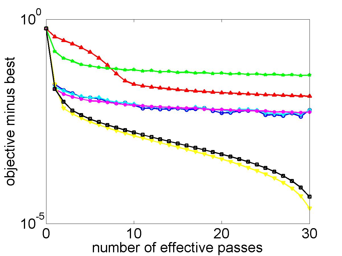
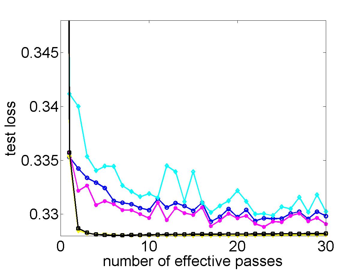
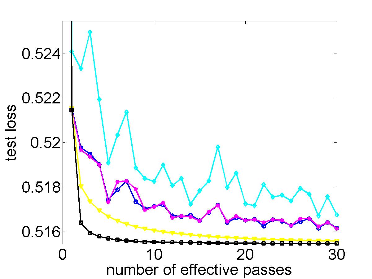
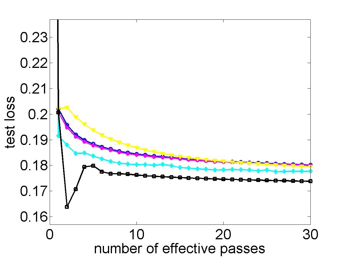
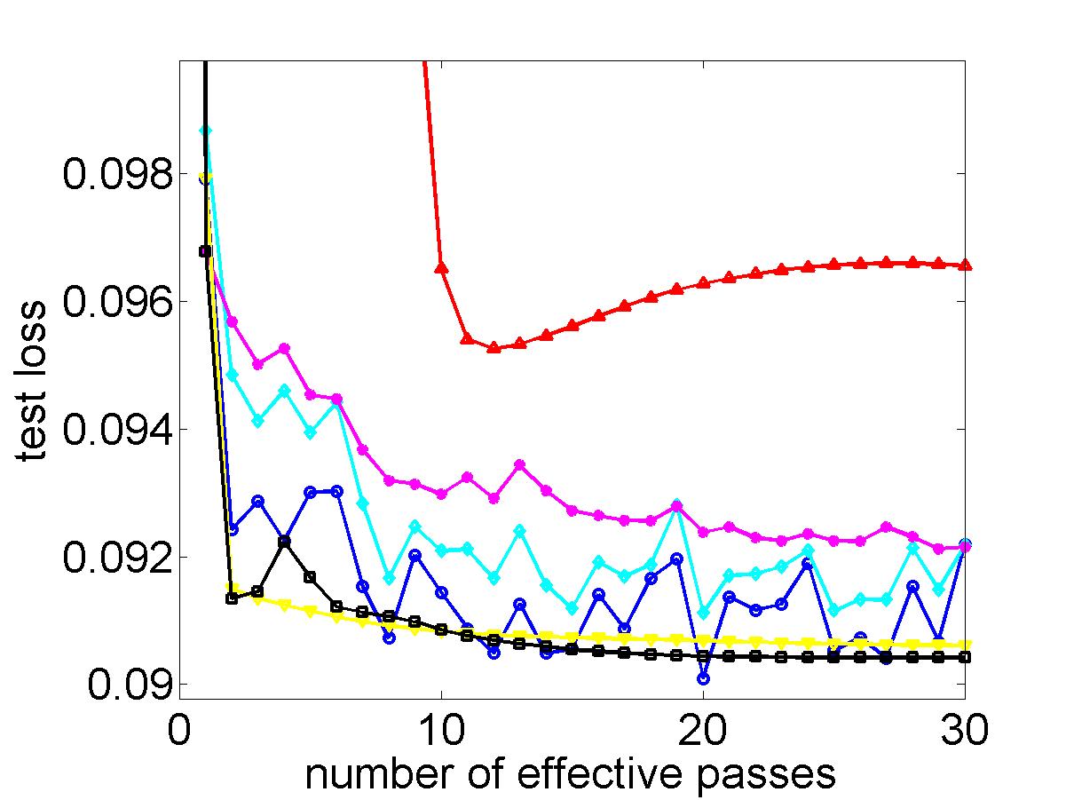
Experiments are performed on five binary classification data sets: a9a, covertype, quantum, rcv1, and sido (Table II), which have been commonly used [14, 6]. For each data set, half of the samples are used for training, while the rest for testing. To reduce statistical variability, results are averaged over 10 repetitions. We fix $\rho$ in (3) to $0.01$; and the regularization parameter $\lambda$ to $10^{-5}$ for a9a, covertype, quantum, and to $10^{-4}$ for rcv1 and sido. For selection of stepsize (or its proportionality constant), we run each stochastic algorithm 5 times over a small training subset (with 500 samples) and choose the setting with the smallest training objective value. For each batch algorithm, we run it for 100 iterations on the same training subset. All methods are implemented in MATLAB.

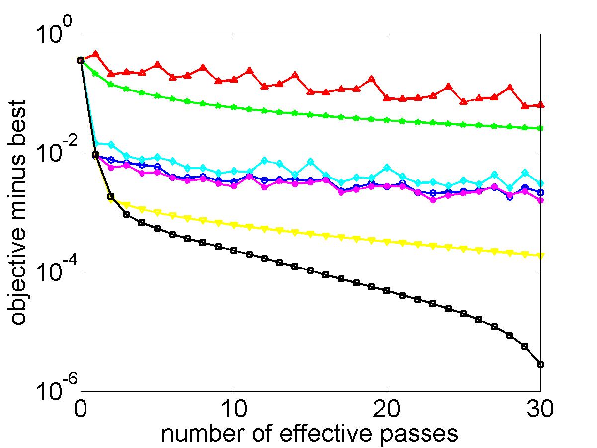
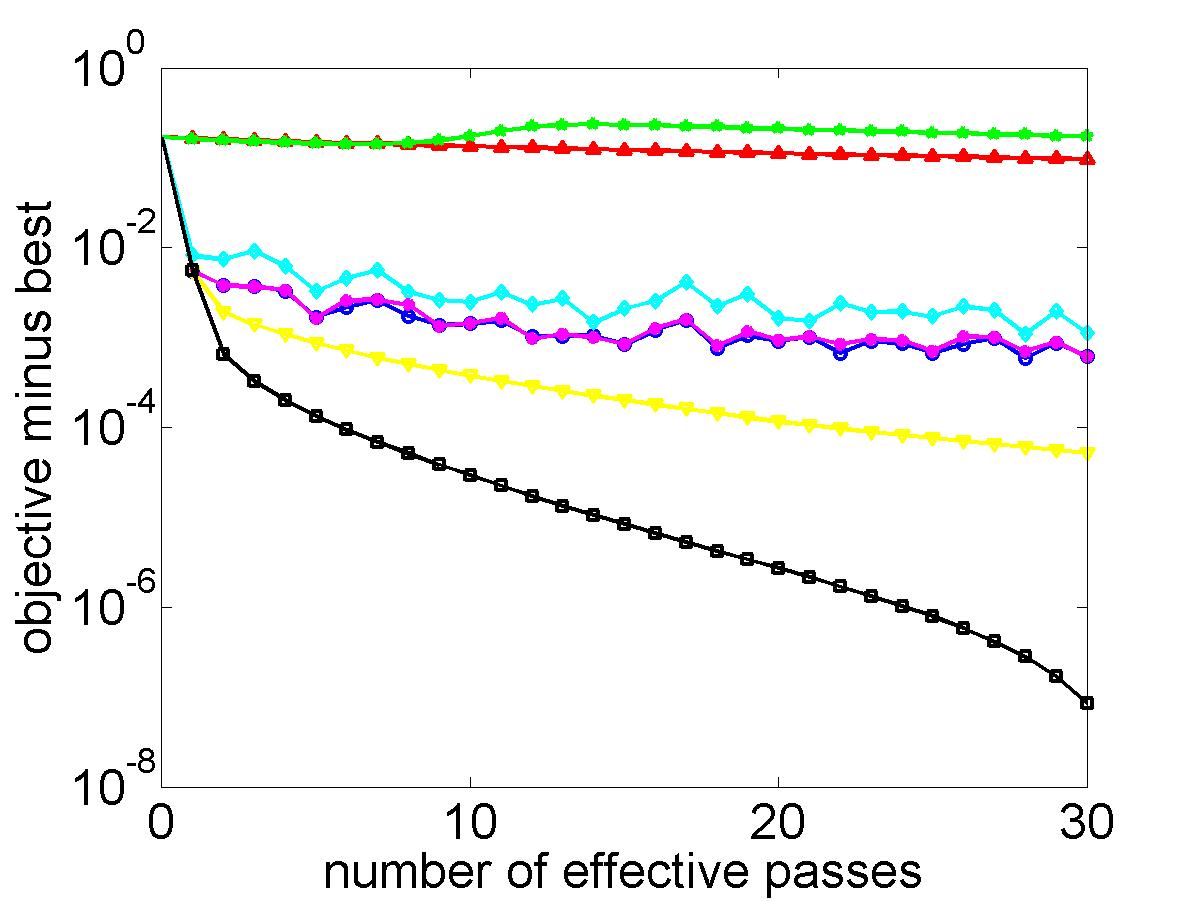
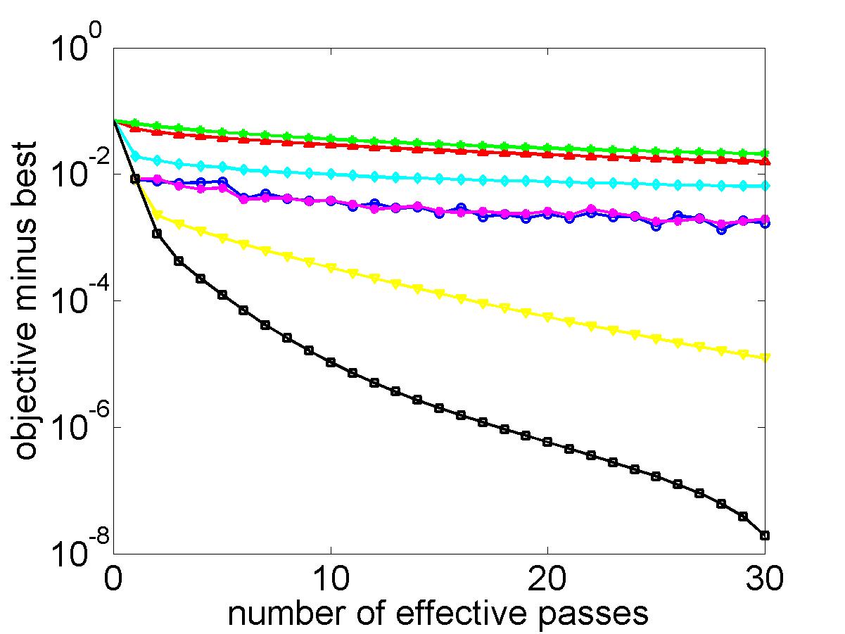
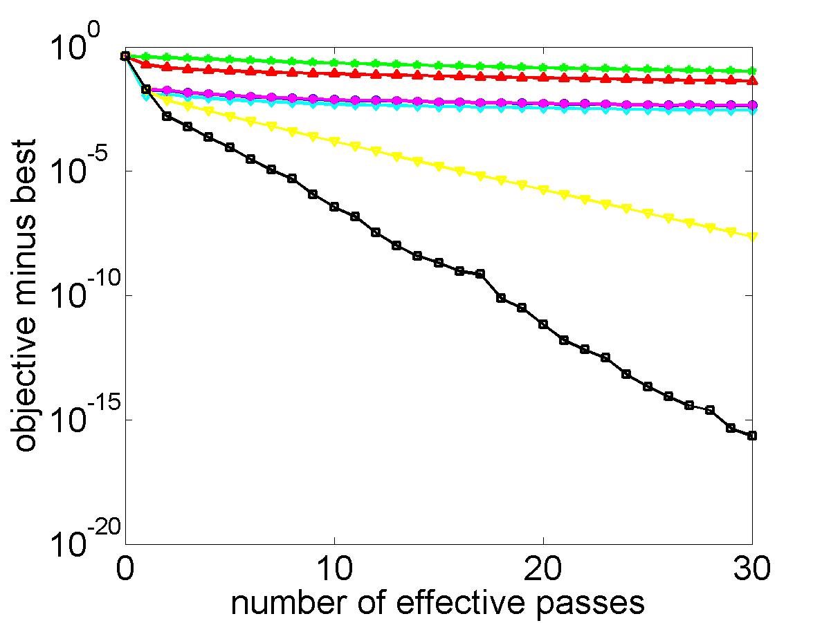
Figures 1 and 2 show the objective value and testing loss versus the number of effective passes over the data. Overall, SA-IU-ADMM is the fastest, which is followed by SA-ADMM, and then the other stochastic algorithms. The batch ADMM algorithms are the slowest.

(a) a9a

(b) covertype

(c) quantum

(d) rcv1

(e) sido

Figure 2: Testing loss versus number of effective passes.

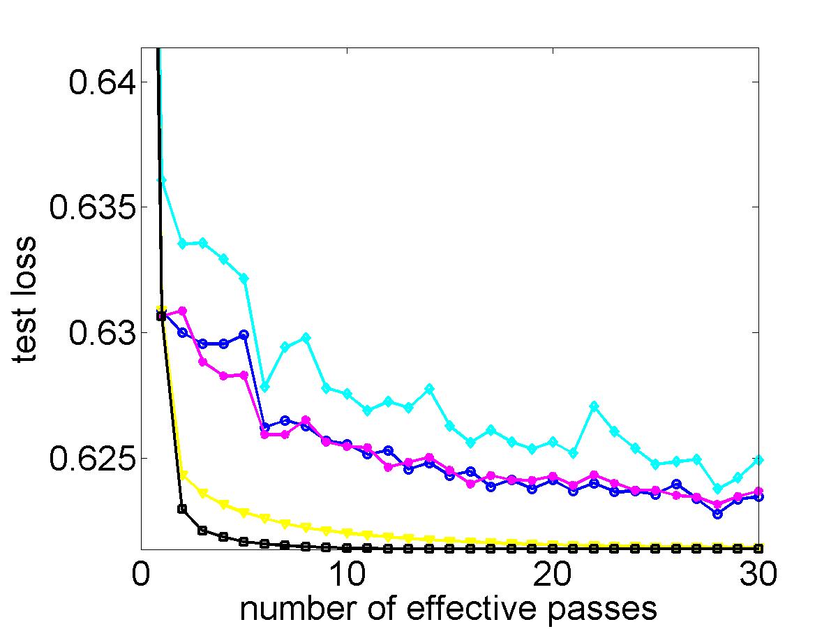
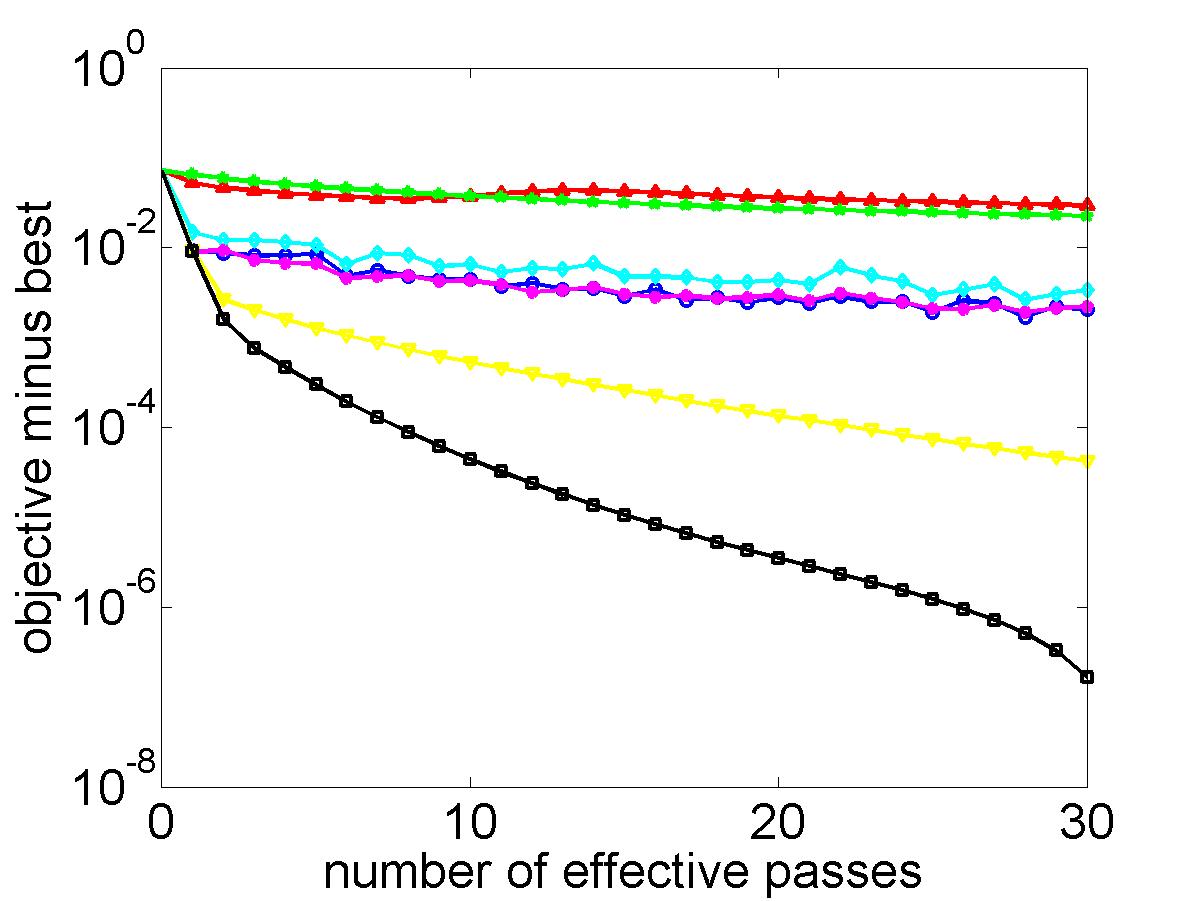
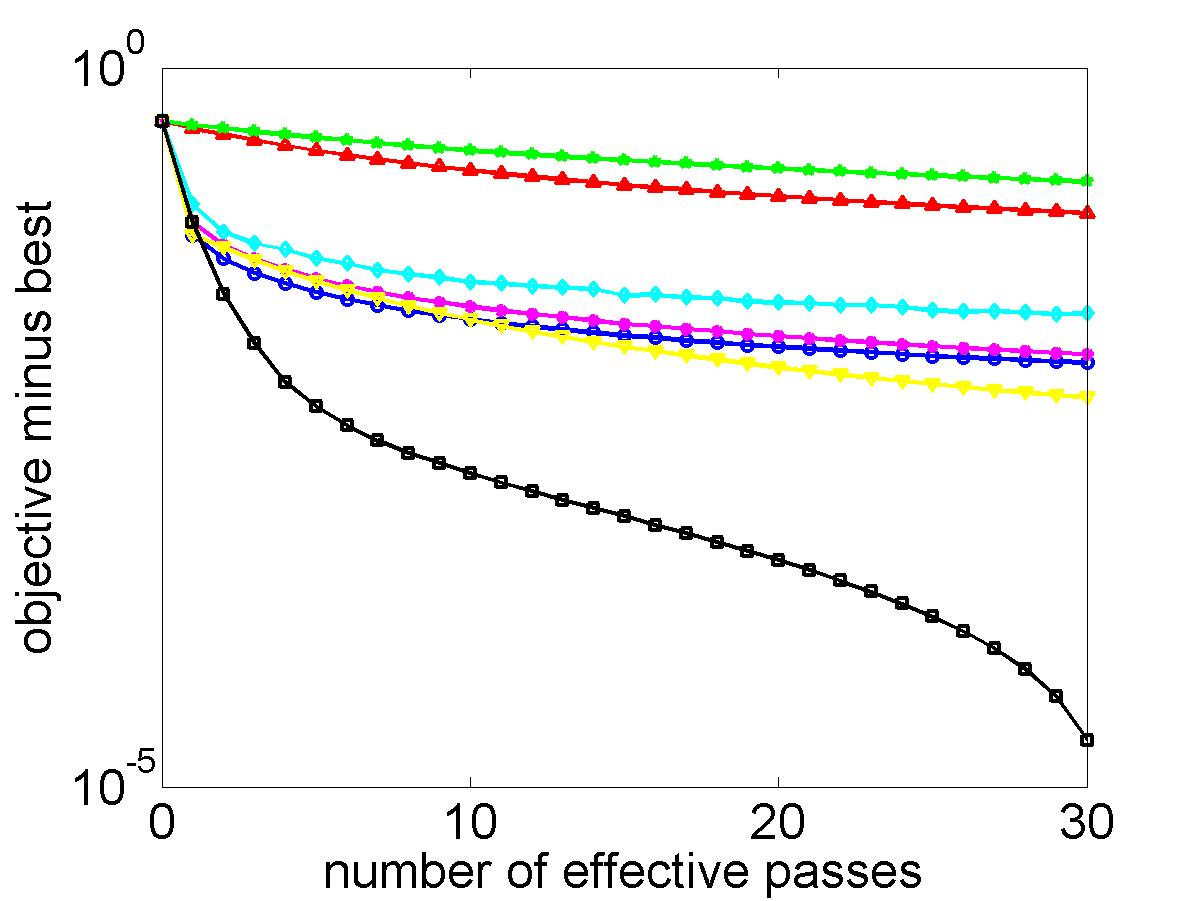
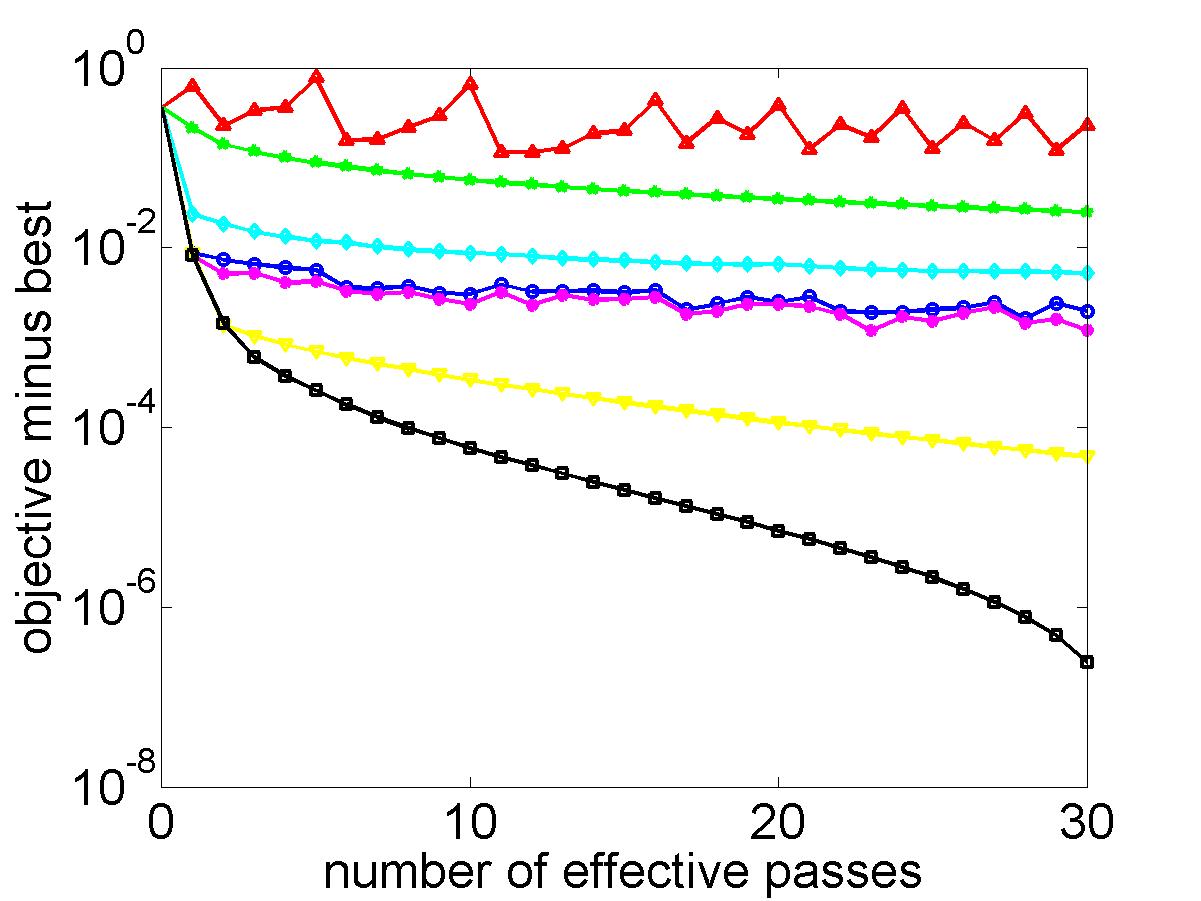
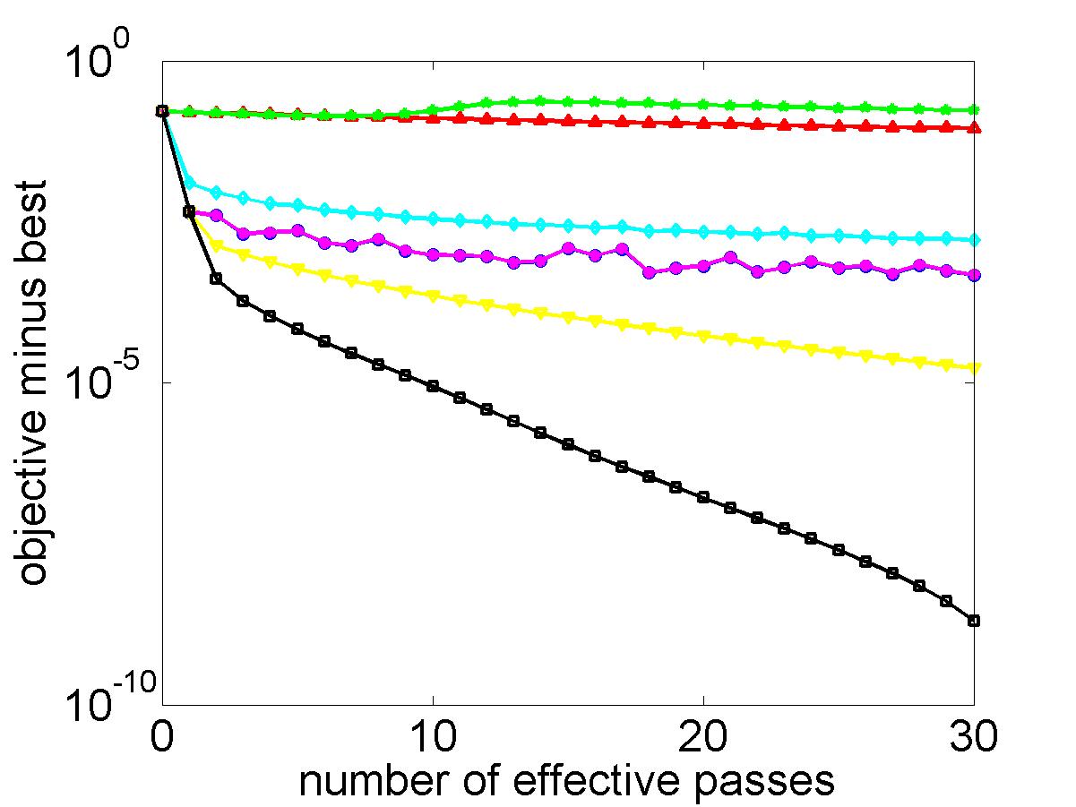
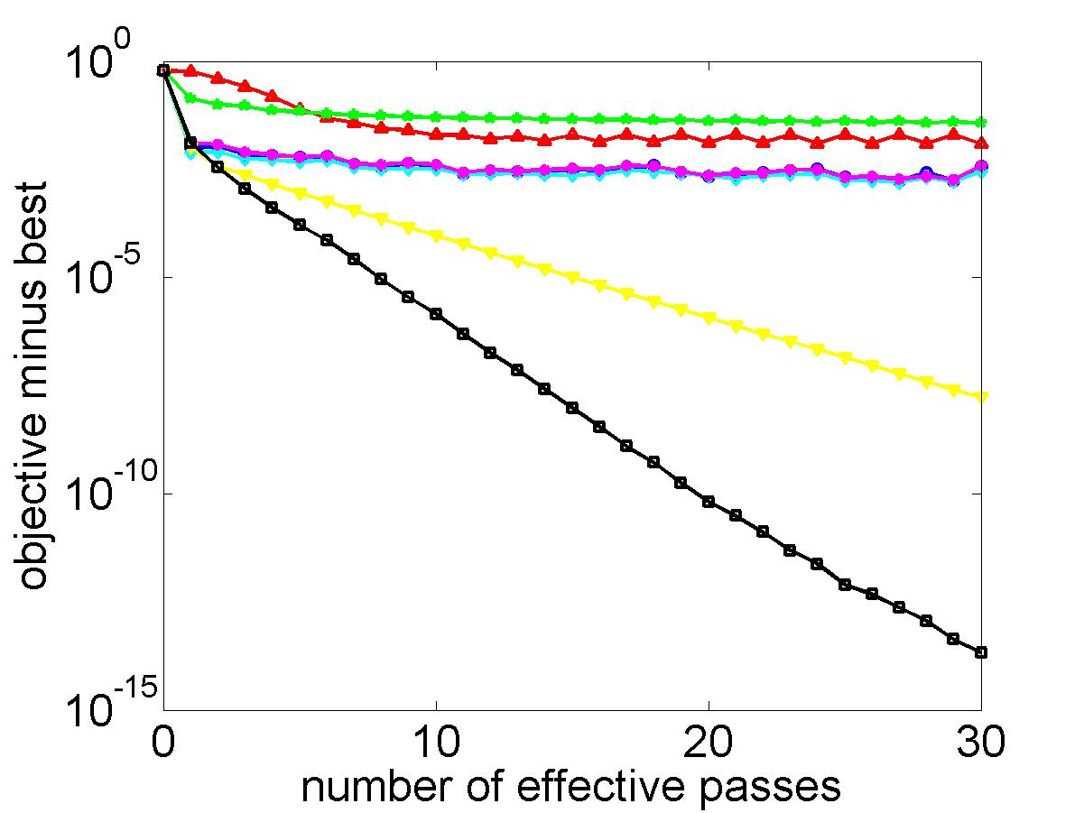
As discussed in Section II, STOC-ADMM and OPG-ADMM has $\mathcal{O}(\log T/T)$ convergence when the loss is strongly convex. It is still an open question whether this also holds for the proposed algorithm. In the following, we will compare their performance empirically by adding an extra $\ell_{2}$-regularizer on $x$. Results are shown in Figure 3. As can be seen, the improvement of SA-IU-ADMM over others is even more dramatic.

(a) a9a

(b) covertype

(c) quantum

(d) rcv1

(e) sido

Figure 3: Objective value versus number of effective passes for the strongly convex problem.

V Conclusion

In this paper, we developed a novel stochastic algorithm that incrementally approximates the full gradient in the linearized ADMM formulation. It enjoys the same computational simplicity as existing stochastic ADMM algorithms, but has a fast convergence rate that matches the batch ADMM. Empirical results on both general convex and strongly convex problems demonstrate its efficiency over batch and stochastic ADMM algorithms. In the future, we will investigate the theoretical convergence rate of the proposed algorithm on strongly convex problems.

References

- [1] S. Boyd, “Distributed optimization and statistical learning via the alternating direction method of multipliers,” Foundations and Trends in Machine Learning, vol. 3, no. 1, pp. 1–122, 2010.
- [2] D. Gabay and B. Mercier, “A dual algorithm for the solution of nonlinear variational problems via finite element approximation,” Computers & Mathematics with Applications, vol. 2, no. 1, pp. 17–40, 1976.
- [3] R. Glowinski and A. Marrocco, “Sur l’approximation, par elements finis d’ordre un, et la resolution, par penalisation-dualite, d’une classe de problems de dirichlet non lineares,” Revue Francaise d’Automatique, Informatique, et Recherche Opérationelle, vol. 9, pp. 41–76, 1975.
- [4] J. Duchi and Y. Singer, “Efficient online and batch learning using forward backward splitting,” Journal of Machine Learning Research, vol. 10, pp. 2873–2908, 2009.
- [5] L. Xiao, “Dual averaging methods for regularized stochastic learning and online optimization,” Journal of Machine Learning Research, vol. 11, pp. 2543–2596, 2010.
- [6] T. Suzuki, “Dual averaging and proximal gradient descent for online alternating direction multiplier method,” in Proceedings of the 30th International Conference on Machine Learning, Atlanta, GA, USA, 2013, pp. 392–400.
- [7] Z. Qin and D. Goldfarb, “Structured sparsity via alternating direction methods,” Journal of Machine Learning Research, vol. 13, pp. 1435–1468, 2012.
- [8] H. Wang and A. Banerjee, “Online alternating direction method,” in Proceedings of the 29th International Conference on Machine Learning, Edinburgh, Scotland, UK, July 2012, pp. 1119–1126.
- [9] H. Ouyang, N. He, L. Tran, and A. Gray, “Stochastic alternating direction method of multipliers,” in Proceedings of the 30th International Conference on Machine Learning, Atlanta, GA, USA, 2013.
- [10] L. Bottou, “Stochastic learning,” in Advanced Lectures on Machine Learning. Springer Verlag, 2004, p. 146–168.
- [11] W. Deng and W. Yin, “On the global and linear convergence of the generalized alternating direction method of multipliers,” Rice University, Tech. Rep. TR12-14, 2012.
- [12] B. S. He and X. M. Yuan, “On the convergence rate of alternating direction method,” SIAM Journal on Numerical Analysis, vol. 22, no. 4, pp. 1431–1448, 2012.
- [13] J. Mairal, “Optimization with first-order surrogate functions,” in Proceedings of the 30th International Conference on Machine Learning, Atlanta, GA, USA, 2013.
- [14] N. Le Roux, M. Schmidt, and F. Bach, “A stochastic gradient method with an exponential convergence rate for finite training sets,” in Advances in Neural Information Processing Systems 25, 2012, pp. 2672–2680. [Online]. Available: http://books.nips.cc/papers/files/nips25/NIPS2012_1246.pdf
- [15] S. Shalev-Shwartz and T. Zhang, “Proximal stochastic dual coordinate ascent,” arXiv:1211.2717, 2013.
- [16] X. Zhang, M. Burger, and S. Osher, “A unified primal-dual algorithm framework based on Bregman iteration,” Journal of Scientific Computing, vol. 46, no. 1, pp. 20–46, Jan. 2011.
- [17] M. Hong and Z.-Q. Luo, “On the linear convergence of the alternating direction method of multipliers,” University of Minnesota, Tech. Rep. arXiv:1208.3922, 2012.
- [18] F. Bach, R. Jenatton, J. Mairal, and G. Obozinski, “Convex optimization with sparsity-inducing norms,” in Optimization for Machine Learning, S. Sra, S. Nowozin, and S. Wright, Eds. MIT Press, 2011, pp. 19–53.
- [19] A. Beck and M. Teboulle, “A fast iterative shrinkage-thresholding algorithm for linear inverse problems,” SIAM Journal on Imaging Sciences, vol. 2, no. 1, pp. 183–202, 2009.
- [20] R. J. Tibshirani and J. Taylor, “The solution path of the generalized lasso,” Annals of Statistics, vol. 39(3), pp. 1335–1371, 2011.
- [21] S. Kim, K.-A. Sohn, and E. Xing, “A multivariate regression approach to association analysis of a quantitative trait network,” Bioinformatics, vol. 25, no. 12, pp. i204–i212, 2009.
- [22] O. Banerjee, L. El Ghaoui, and A. d’Aspremont, “Model selection through sparse maximum likelihood estimation for multivariate Gaussian or binary data,” Journal of Machine Learning Research, vol. 9, pp. 485–516, 2008.
- [23] A. Barbero and S. Sra, “Fast Newton-type methods for total variation regularization,” in Proceedings of the 28th International Conference on Machine Learning, New York, NY, USA, Jun. 2011, pp. 313–320.
- [24] J. Liu, L. Yuan, and J. Ye, “An efficient algorithm for a class of fused lasso problems,” in Proceedings of the 16th International Conference on Knowledge Discovery and Data Mining, 2010, pp. 323–332.