An Efficient Coarse Grid Projection Method for Quasigeostrophic Models of Large-Scale Ocean Circulation
Abstract
This paper puts forth a coarse grid projection (CGP) multiscale method to accelerate computations of quasigeostrophic (QG) models for large scale ocean circulation. These models require solving an elliptic sub-problem at each time step, which takes the bulk of the computational time. The method we propose here is a modular approach that facilitates data transfer with simple interpolations and uses black-box solvers for solving the elliptic sub-problem and potential vorticity equations in the QG flow solvers. After solving the elliptic sub-problem on a coarsened grid, an interpolation scheme is used to obtain the fine data for subsequent time stepping on the full grid. The potential vorticity field is then updated on the fine grid with savings in computational time due to the reduced number of grid points for the elliptic solver. The method is applied to both single layer barotropic and two-layer stratified QG ocean models for mid-latitude oceanic basins in the beta plane, which are standard prototypes of more realistic ocean dynamics. The method is found to accelerate these computations while retaining the same level of accuracy in the fine-resolution field. A linear acceleration rate is obtained for all the cases we consider due to the efficient linear-cost fast Fourier transform based elliptic solver used. We expect the speed-up of the CGP method to increase dramatically for versions of the method that use other, suboptimal, elliptic solvers, which are generally quadratic cost. It is also demonstrated that numerical oscillations due to lower grid resolutions, in which the Munk scales are not resolved adequately, are effectively eliminated with CGP method.
Keywords:Coarse grid projection, multigrid, forced-dissipative quasigeostropic ocean models, large-scale ocean circulation, single-layer barotropic model, two-layer stratified model, climate modeling.
1 Introduction
Oceanic and atmospheric flows display an enormous range of spatial and temporal scales, from seconds to decades and from centimeters to thousands of kilometers. Scale interactions, both spatial and temporal, are the dominant feature of all aspects of general circulation models in geophysical fluid dynamics (Klein, 2010; Hurrell et al., 2009) and bridging the scales in geophysical systems is of paramount importance in numerous critical areas and industries. Atmospheric and oceanic flows have intrinsic complex multiscale interactions. The accurate and efficient numerical simulation of these geophysical flows is of great importance in weather and climate models and could perhaps benefit from a dedicated investigation of the application of classes of modern multiscale modeling and simulation (MMS) methods (Brandt, 2002; Barth et al., 2002; Fish, 2009; E, 2011), which exploit vastly different temporal and spatial scales in problems in order to speed up their computations. Similar to the parallel developments in applied mathematics and engineering science, interest in the development and testing of the MMS methods in geophysical flow settings has increased in recent years (Iskandarani et al., 2002; Majda and Klein, 2003; Khairoutdinov et al., 2008; Alam, 2011; Campin et al., 2011; Ringler et al., 2011), leading to several successful applications and research efforts at numerous weather and climate centers. The MMS framework could provide a significant increase in the accuracy and computational efficiency of numerous interconnected physical oceanic and atmospheric flow models for advanced numerical weather prediction, data assimilation and climate modeling strategies.
The ocean is a forced-dissipative fluid system, with forcing largely at the boundaries and dissipation at the molecular scale. The investigation of characteristics of the forced-dissipative ocean circulation models is of primary importance in developing our understanding of the complex large-scale nonlinear motions of large-scale oceanic flows that move in great circular sweeps (called “gyres”). As one of the main circulation sources, most of the surface currents in the ocean are shaped by wind, which drives the general circulation associated with the subtropical and subpolar gyres, which can be identified with the strong, persistent, sub-tropical and sub-polar western boundary currents in the North Atlantic Ocean (the Gulf Stream and the Labrador Current) and North Pacific Ocean (the Kuroshio and the Oyashio Currents) and sub-tropical counterparts in the southern hemisphere (Stommel, 1972; Kelly et al., 2010). One of the major similarities between the various ocean basins is the asymmetry of the gyres: strong western boundary currents and weaker flow in the interior; weak and shallow eastern boundary currents. The most obvious motivation for being interested in forced-dissipative wind-driven ocean circulation is the connection between ocean currents and climate dynamics (Ghil et al., 2008; Lynch, 2008; Stocker, 2011).
Ocean eddies have a horizontal scale of typically several hundred kilometers and are often much stronger than the mean flow, leading to a highly turbulent, chaotic flow. The mean pattern of currents only emerges after averaging over many years. The wind-driven circulation in an enclosed, midlatitude rectangular or square oceanic basin is a classical problem in physical oceanography, studied extensively by modelers (Allen, 1980; Holland and Rhines, 1980; Griffa and Salmon, 1989; Vallis, 2006; Miller, 2007). To decrease the computational cost required for an accurate representation of large-scale oceanic flows, several class of simplified models are derived from the full-fledged equations of geophysical flows, Boussinesq equations (BEs) or the primitive equations (PEs), to guide the theoretical studies on boundary currents, alternating zonal flows, or jet formations, as well as to identify some key issues related to the robustness of the model dynamics to the changes of parameters that is closely linked to a dynamical system point of view (Speich et al., 1995; Meacham, 2000; Chang et al., 2001; Nauw et al., 2004; Dijkstra, 2005; Dijkstra and Ghil, 2005). The quasigeostropic (QG) model is a simplification of the primitive equation model that retains many of the essential features of geophysical fluid flows. Details of the mathematical and physical approximations may be found in standard textbooks on geophysical fluid dynamics, such as Pedlosky (1987), Vallis (2006), and McWilliams (2006). The main assumptions that go into the QG models are: the hydrostatic balance, the -plane approximation (i.e., the variation of the Coriolis parameter with latitude), the geostrophic balance, and the eddy viscosity parameterization. Despite the fact that the QG models are a simplified version of the full-fledged equations of geophysical flows, their numerical simulation is still computationally challenging when long-time integration is required, as is the case in climate modeling.
The barotropic vorticity equation (BVE) represents one of the most commonly used mathematical models for this type of geostrophic flows with various dissipative and forcing terms (Majda and Wang, 2006). In reality, the ocean is a stratified fluid on a rotating Earth driven from its upper surface by patterns of momentum and buoyancy fluxes (Marshall et al., 1997). While the barotropic model is not stratified, it exhibits many of the features that are observed in the stratified case. To explore some of the effects of the stratification, the one-layer barotropic equation can be extended to the 1.5-layer model, also called the reduced gravity QG model (Özgökmen et al., 2001). There are two layers in this model, but the second layer is infinitely deep and at rest (passive), and the dynamics are effectively barotropic. The two-layer model takes the next step in increasing the complexity of stratification by adding a second dynamically active layer (Holland, 1978; Özgökmen and Chassignet, 1998; Berloff and McWilliams, 1999; DiBattista and Majda, 2001; Berloff et al., 2009). The dynamics in this model include the first baroclinic modes. The complexity of the models could be increased by adding more active layers, resulting in the N-layer models (Siegel et al., 2001), which, in turn, yield the three dimensional primitive equations when N goes to infinity (McWilliams, 2006). In this study, we use both the one-layer quasigeostropic (QG1) and two-layer quasigeostropic (QG2) models.
Although large-scale ocean dynamics are well represented by QG ocean models, primitive equation models have been used in state of art weather prediction softwares. Several reasons have been addressed for the recent lack of popularity in of these quasigeostropic models (Miller, 2007). One is the ready availability of full-fledged primitive equation codes on the web, but that is not the only reason. There is a need for computational strategies that can significantly decrease the computational cost of the geophysical models without compromising their physical accuracy. Large eddy simulation (LES) approaches appear as a natural choice to accelerate the simulation on coarser grid in which the subgrid scale terms are modeled to capture the under-resolved flow, i.e., the flow in the regions where the grid size becomes greater than the specified Munk scale. San et al. (2011) proposed an approximate deconvolution large eddy simulation technique for one-layer barotropic quasiqeostropic large-scale ocean model. It was shown that the approximate deconvolution model provides an accurate approximation for under-resolved subfilter-scale effects.
Here, we approach to the problem from a different point of view. Instead of filtering the governing equations and modeling underresolved quantities on a coarser grid, we separate the problem to two parts based on the nature of the QG models: (i) the elliptic sub-problem and (ii) the potential vorticity evolution. Most of the demand on computational resources by QG models comes in the solution of the elliptic inversion sub-problem which states the relationship between the potential vorticity and stream function. The natural advantages of QG models may well lead to increased application when efficient methods available for elliptic sub-problem. One straightforward way to accelerate QG simulations is to reduce the number of grid points for the most time consuming part of the problem, the elliptic sub-problem. Previous studies have demonstrated that scale dependant computational slowness can be overcome by multiscale and multiresolution algorithms (Brandt, 2005). Along this direction, the coarse grid projection (CGP) framework was proposed by Lentine et al. (2010) and successfully applied to three-dimensional incompressible flow simulations by coarsening the number of grid points for the Poisson equation. A systematic error analysis on the coarse grid projection method has been recently performed by San and Staples (2012) for Navier-Stokes equations. The main goal of this report is to extend the CGP approach to the QG large scale ocean circulation models. The cost of the flow computations is reduced by coarsening the resolution of the numerical grid on which the elliptic sub-problem is solved by factors of two in each direction according to , where is the fine resolution of the numerical grid on which the potential vorticity equation is solved, and is the coarse resolution for the solution of the elliptic sub-problem. When no coarsening is applied and the CGP method reduces to the underlying standard QG solver. In our numerical investigations, we serendipitously discovered that the CGP procedure can actually predict the fine level simulation details without loss of accuracy for a reduced computational cost.
The coarse grid projection methodology is a modular approach that facilitates data transfer with simple restriction and prolongation interpolations and uses black-box solvers for the advection-diffusion and elliptic parts of the QG models. A particular version of the method is applied here using a third-order Runge-Kutta method for advection-diffusion part and a fast Fourier transform based direct solver for the elliptic part. The full weighting operation for mapping from the fine to coarse grids is used to obtain the data for the elliptic sub problem. After solving the elliptic part on a coarsened grid, bilinear interpolation is used to obtain the fine data for consequent time stepping on the full grid. Similar mapping operators have been used in multigrid algorithms (Brandt, 1977; Hackbusch, 1985; Briggs et al., 2000; Trottenberg et al., 2001). The efficiency of the interpolation based methods highly depends on the interpolation scheme (Fish and Chen, 2004), and has been substantially investigated in the multigrid literature. Since we are using a second-order spatial discretization scheme, however, the full weighting operator for the restriction and bilinear interpolation for the prolongation are consistent and efficient for our study. The mapping procedures used in this study could potentially be improved by introducing higher-order spline formulas, or more advanced methods for deriving interpolations (Lee et al., 1997; Höllig et al., 2002; Brezina et al., 2005; Brandt, 2010). The coarse grid projection approach proposed here can be classified within the systematic upscaling methodologies that have been used in the context of the multigrid/multiresolution branch of multiscale methods.
The rest of the paper is organized as follows: Both barotropic one-layer BVE and two-layer stratified QG models, the mathematical models used in this report, are presented in Section 2. Section 3 presents the coarse grid projection methodology for these QG models. The numerical methods used in our simulations are briefly discussed in Section 4. The results for the new CGP method for the large-scale ocean models are presented in Section 5. Finally, the conclusions are summarized in Section 6.
2 Mathematical Models
In this section, we present the quasigeostropic models used in the numerical investigation of the proposed coarse grid projection method for large scale ocean circulation. We first present the BVE which is one of the most used mathematical models for geostrophic flows with various dissipative and forcing terms (Majda and Wang, 2006). Next, we present the two-layer QG model which is the simple extension of single-layer barotropic model to the stratified ocean by including another active layer.
2.1 One-layer barotropic model
In this section, we present the BVE, one of the most used mathematical models for forced-dissipative large scale ocean circulation problem. Studies of wind-driven circulation using an idealized double-gyre wind forcing have played an important role in understanding various aspects of ocean dynamics, including the role of mesoscale eddies and their effect on mean circulation. Following Greatbatch and Nadiga (2000), we briefly describe the BVE. For more details on the physical mechanism and various formulations utilized, the reader is referred to Greatbatch and Nadiga (2000); Munk and Wunsch (1982); Cummins (1992); Nadiga and Margolin (2001); Fox-Kemper (2005).
The barotropic vorticity equation for one-layer quasigeostropic forced-dissipative ocean model can be written as
| (1) |
where and represent the dissipation and forcing terms, respectively. In Eq. (18), is the potential vorticity, defined as
| (2) |
where is the gradient of the Coriolis parameter at the basin center (). Here, is the local vorticity, the curl of the velocity field, and the kinematic relationship between the vorticity and the stream function yields the following definition
| (3) |
in which is the Laplacian operator, and symbolizes the velocity stream function. Flow velocity components can be found from the stream function:
| (4) |
The nonlinear convection term in Eq. (18), called the Jacobian, is defined as
| (5) |
The viscous dissipation in Eq. (18) has the form
| (6) |
where is the uniform eddy viscosity coefficient. Viscous term can be written in terms of stream function in the following form
| (7) |
The double-gyre wind forcing is given by
| (8) |
where is the maximum amplitude of double-gyre wind stress, is the mean density, and is the mean depth of the ocean basin. In order to nondimensionalize the BVE equation we use the following definitions
| (9) |
where the tilde denotes the corresponding dimensional variables. In the nondimensionalization, represents the characteristic horizontal length scale (i.e., in our study is the basin dimension in direction), and represents the characteristic velocity scale. The Sverdrup velocity scale used for nondimensionalization can be written in the follwing form:
| (10) |
Finally, the governing equations for two-dimensional incompressible barotropic flows can be written in dimensionless form of the potential vorticity formulation in the beta plane as the BVE:
| (11) |
where is the Munk scale. The elliptic sub-problem which relates the potential vorticity and stream function becomes
| (12) |
where is defined as Rhines scale. In dimensionless form, there are only two physical parameters, the Rhines scale and the Munk scale, which are related to the physical parameters in the following way:
| (13) |
The physical parameters in the BVE (18), the Rhines scale and the Munk scale , are related to the Reynolds and Rossby numbers through the following formulas:
| (14) |
| (15) |
where Ro is the Rossby number and Re is the Reynolds number based on the basin dimension, . We note that some authors use a boundary layer Reynolds number, which is written as
| (16) |
where for oceanic flows Fox-Kemper (2005). Finally, in order to completely specify the mathematical model, boundary and initial conditions need to be prescribed. In many theoretical studies of large scale ocean circulation, slip or no-slip boundary conditions are used. Following these studies Greatbatch and Nadiga (2000); Nadiga and Margolin (2001); Holm and Nadiga (2003); Cummins (1992); Munk (1950); Bryan (1963), we use slip boundary conditions for the velocity, which translate into homogenous Dirichlet boundary conditions for the vorticity: . The impermeability boundary condition is imposed as . For the initial condition, we start our computations from a quiescent state and integrate Eq. (18) until a statistically steady state is obtained in which the wind forcing, dissipation, and Jacobian balance each other.
2.2 The two-layer quasigeostrophic equations
The two-layer quasigeostrophic model used in this study is one of the simplified forced-dissipative oceanic models that considers baroclinic effects. The stratified ocean is partitioned into two isopycnal layers, each of constant depth, density and temperature. The governing quasigeostrophic potential vorticity equations for the two dynamically active layers are (Pedlosky, 1987; Salmon, 1998; McWilliams, 2006)
| (17) | |||||
| (18) |
where the layer index starts from top, represents potential vorticities, and denotes for streamfunctions. The dissipation and forcing (Ekman pumping) terms are represented by , and , respectively. The potential vorticities for each layer are related to the velocity streamfunctions through the following elliptic coupled system of equations:
| (19) | |||||
| (20) |
The isopycnal flow velocity components can be found from the velocity streamfunctions:
| (21) |
The two symbols and are parts of the linearized -plane approximation to the Coriolis parameter . Here is the local rotation rate at , where is the rotational speed of the earth and is the latitude at . This is equivalent to approximating the spherical Earth with a tangent plane at . Stratification is represented by two stacked isopycnal layers with thicknesses and , starting from the top, and is reduced gravity associated with the density jump between the two layers in which is the density difference between the two layers, is the reference (upper layer) density, and is the gravitational acceleration. The inertial radius of deformation between layers, a measure of stratification strength, is defined as the Rossby deformation radius , where . In this study, the top and bottom layers of the ocean are forced by an Ekman pumping of the form
| (22) | |||||
| (23) |
where is the stress vector for surface wind forcing, and is unit vector in vertical direction. In the present model, we use a double-gyre wind forcing only for zonal direction: , where is the meridional length of the ocean basin centered at , and is the maximum amplitude of the wind stress. This form of wind stress represents the meridional profile of easterly trade winds, mid-latitude westerlies, and polar easterlies from South to North. The bottom Ekman layer is parameterized by a linear bottom friction with coefficient . In the equations above, and are the gradient and Laplacian operators, respectively. For the dissipation terms, the following EV parameterizations are used:
| (24) | |||||
| (25) |
where is eddy viscosity coefficient. Similar to the previous analysis, the governing equations can be written in dimensionless form by using the Sverdrup balance to set the velocity scale of the form
| (26) |
Then the two-layer quasigeostrophic equations in dimensionless form become
| (27) | |||||
| (28) |
In dimensionless form, the kinematic relationships between potential vorticities and streamfunctions yield the following elliptic sub-problem:
| (29) | |||||
| (30) |
For clarity of exposition, in the remainder of the paper we will drop the tilde symbol used for the dimensionless variables. In the two-layer QG model, is the aspect ratio of vertical layer thicknesses, Ro is the Rossby number, Fr is the Froude number, is the lateral eddy viscosity coefficient, and is the Ekman bottom later friction coefficient. The definitions of these dimensionless parameters are:
| (31) |
The following three length scales are useful for setting the two-layer problem parameters: (i) the Munk scale, , for the viscous boundary layer; this is related to the smaller scale dissipation; (ii) the Stommel scale, , for the bottom boundary layer thickness; this is accounting for larger scale damping; and (iii) the Rhines scale, , for the inertial boundary layer; this is measuring the strength of the nonlinearity.
In order to complete the mathematical model, boundary and initial conditions should be prescribed. In many theoretical studies of ocean circulation, the modelers either use free-slip boundary conditions or no-slip boundary conditions. Following Cummins (1992); Özgökmen and Chassignet (1998), we use free-slip boundary conditions for the velocity for both isopycnal layers, which translates into homogenous Dirichlet boundary conditions for the vorticity (Laplacian of streamfunction): . The impermeability boundary condition is imposed as . Similar to the one-layer problem, we start from a rest state, integrate the model until a statistically steady state is obtained, and continue for several decades to compute time-averaged results.
3 Coarse Grid Projection
In QG models solving the elliptic sub-problem takes considerably more computational time than solving the time dependent part (i.e., potential vorticity evolution equation) of the problem. Within each time step, solving the time dependant part of the problem is usually of where “” is the number of degrees of freedom (total grid points, for one-layer setting and for two-layer setting) of the problem. In general, the alternating direction implicit (ADI), Gauss-Seidel (GS) or successive over relaxation (SOR) types of iterative algorithms for solving the elliptic equation are of (Saad, 2003). The practical consequence is that it is not feasible to use these types of iterative elliptic solvers for high resolution (and therefore high Reynolds number) computations along with long time integration. In order to accelerate these solvers, very successful multigrid algorithms have been developed that reduce the computational effort to close to where is a proportionality constant (Wesseling, 2004; Gupta et al., 1997; Zhang, 1998). On the other hand, for certain ideal problems on equally-spaced grids, fast Fourier transform (FFT) based fast Poisson solvers can be used that are , and are presently the fastest algorithms ( in the relevant resolutions) for solving Poisson equations (Moin, 2001). The computational efficiencies of different elliptic solvers are shown in Fig. (1) for solving a standard Poisson equation on a square domain with equidistant grid spacing. This preliminary comparison shows that FFT based elliptic solver is the most efficient solver for our sub-problems in the QG models. The computational gains in the CGP method are directly related to selection of the elliptic solver. We have intentionally selected most efficient linear-cost elliptic solver to show the concept. We highlight that any computational gain obtained with this optimal linear-cost FFT based elliptic solver would be more immense if we used some other sub-optimal iterative type elliptic solver.
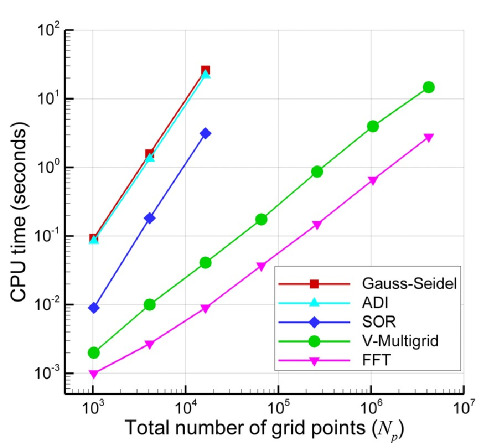
The basic idea behind coarse grid projection (CGP) is to use a smaller number of grid points for solving the elliptic sub-problem. The CGP approach we propose here is modular and independent of the elliptic solver that is used. As shown by our preliminary analysis for solving Poisson equation, usually FFT based elliptic solvers are optimal for rectangular domain problems because they are fast and have minimal storage requirements. They are preferred because of their efficiency when using orthogonal coordinate systems in which there are no mixed derivatives. The general domains treated with body-fitted coordinates are out of bounds for FFT solvers due to the presence of mixed derivatives in the transformed generalized curvilinear coordinates. In that case, the V-cycle multigrid solver becomes the optimal elliptic solver to use. Since we used Drichlet type boundary conditions (i.e., free-slip boundary contions) for our oceanic basins, a fast sine transform are utilized which we will briefly address on the following section where we present the numerical methods.
Even though we use the fastest elliptic solver available for our computations, the most time consuming part of the computations is still solving the elliptic sub-problem. With this in mind, we propose a new multiresolution approach that reduces the number of degrees of freedom for the elliptic solver part of the problem to accelerate the computation. The procedure is as follows: first, we solve the potential vorticity part of the problem using a fine resolution, (the resolution in one direction). Next, we restrict these data to a coarser grid with resolution , where is an integer that determines the level of coarsening ( corresponds to no grid coarsening). After solving the Poisson equation on this coarser grid, we then perform a prolongation of the coarse data to the fine-resolution grid for subsequent time stepping. The procedure can be summarized in the following form:
-
(i)
Compute potential vorticity equation on fine grid
-
(ii)
Map potential vorticity data from fine grid to coarse grid to provide source term for elliptic sub-problem
-
(iii)
Solve elliptic sub-problem for stream function on coarse grid
-
(iv)
Remap stream function data from coarse grid to fine grid, continue to (i) for subsequent time step
We use prolongation and restriction operators between the data for the potential vorticity part and the elliptic sub-problem part of the problem. This seems to be effectively a low-pass filter on the solution to the elliptic sub-problem, similar to the large eddy simulation (LES) methods. However, the concept in CGP is fundamentally different than LES approaches. The philosophy of the LES concept is based on decomposition of the flow variables into resolved and unresolved scales by applying a filter to Navier-Stokes equations (Sagaut, 2006; Berselli et al., 2006). The idea of spatial filtering is central in LES: the large, spatially filtered flow variables are approximated, whereas the effect of the small scales is modeled. This allows for much coarser spatial meshes and thus a computational cost that is significantly lower than that of a direct numerical simulation (DNS). To achieve the same order of physical accuracy as fine resolved DNS, however, LES needs to correctly treat the closure problem: the effect of the small scales on the large ones needs to be modeled. Since the inception of the LES for numerical solution of turbulent flows, substantial effort has been devoted to the turbulence models. These closure models have been suggested to relate the effects of subfilter scales into resolved scales.
On the other hand, the CGP method requires the reduction of degree of freedom just for the most time consuming part of the problem. Although the CGP method can be classified in multigrid methods, the underpinning idea behind CGP is different than the classical multigrid methods. In CGP method we use a smaller number of grid points for solving the most time consuming part of the mathematical model (i.e., elliptic sub-problems in QG models). We demonstrate that it is possible to accelerate simulations without a loss of accuracy by utilizing simple averaging and interpolations between the time dependant part of the solver and the elliptic part. We do this by reducing the size of the problem (via a restriction operation) before we solve the elliptic sub-problem, and solving a smaller sized elliptic system (using any Poisson solver), and then prolongating the results for the consequent time step. We add the costs of the restriction and prolongation operations to the solver, but we save much more computational time in solving the elliptic system because the Poisson equation is solved on a coarser grid. In the classical multigrid approach, the elliptic equation is solved iteratively in such a way that the error in the residual is linearly smoothed. Therefore, it is an optimal linear-cost iterative solution technique for elliptic equations. It doesn’t require changing anything in the existing black-box elliptic solver. The same is true for the algorithm for the time dependant part of mathematical model. Therefore, the multigrid type of elliptic solver can be used in CGP framework. As shown in our preliminary computations for a simple elliptic Possion equation on Cartesian domain, FFT based direct elliptic solver is the most efficient. Since we had chosen only standard oceanic basins on regular Cartesian grids, the FFT-based direct solver became the optimal one for our study. If, instead of using the FFT-based direct solver, we used a multigrid solver, we would see the same speed-up ratios but longer CPU times in the reported results. The speed-up would become larger if we would use a sub-optimal classical solver for the elliptic sub-problem.
3.1 Mapping operators
The only modifications to the standard flow solver computational procedures are the mapping procedures from fine to coarse data and vice versa. In the current study, the full weighting averaging operation is used for data coarsening (restriction), which is given for a two-dimensional equally spaced data array as (Moin, 2001):
| (32) | |||||
where and are the coarse and fine data arrays, and are the coarse grid indices. For almost all multiscale computations, the mapping from the coarse data to the fine data is a critical issue (E et al., 2007; Kevrekidis and Samaey, 2009; Fish, 2009; Wagner et al., 2010). The bilinear interpolation procedure that we use is given for two-dimensional equally spaced grid as:
| (33) |
The half mapping procedures given by Eq. 32 for restriction and Eq. 33 for prolongation can be performed multiple times to obtain different levels of coarsening. The mapping procedure does not take significant computational time compared to the elliptic solver. The mapping procedures used in this study could potentially be improved by introducing higher-order spline formulas. Since we are using a second-order spatial discretization scheme, however, bilinear interpolation is suitable for this study.
3.2 CGP algorithm
The coarse grid projection (CGP) method is independent from the time integration method used. It can be implemented using any time stepping algorithm, for example, the backward difference method, or a method from the Adams-Bashforth or Adams-Moulton families (Schäfer, 2006). Here, the CGP method is used in conjunction with the third-order Runge-Kutta method for the QG models. The joint CGPRK3 algorithm for one-layer barotropic model is presented below. Starting with the value of the potential vorticity, , at the current time step, the CGPRK3 algorithm for computing the potential vorticity at the next time step, , consists of the following steps:
| (34) | |||||
| (35) | |||||
| (36) | |||||
| (37) | |||||
| (38) | |||||
| (39) | |||||
| (40) | |||||
| (41) | |||||
| (42) | |||||
| (43) | |||||
| (44) | |||||
| (45) |
where
| (46) |
The arrows in the algorithm represent the mapping operators. The procedure for the two-layer QG model for stratified flow computations is similar to the one-layer algorithm except that two potential vorticity equations for each isopycnal layer along with a coupled system for elliptic sub-problem are be solved. We will address the solution procedure for the elliptic sub-problem in the following section.
4 Numerical Methods
In many physically relevant situations, where the Munk and Rhines scales being close to each other, the solutions to oceanic models, such as the QG models, do not converge to a steady state as time goes to infinity (Medjo, 2000). Rather they remain time dependent by producing statistically steady state with one or multiple equilibria. Therefore, numerical schemes designed for numerical integration of such phenomena should be suited for such behavior of the solutions and for the long-time integration. In this study, the governing equations are solved by a fully conservative finite difference scheme along with a third-order Runge-Kutta adaptive time stepping algorithm. An efficient, linear-cost, fast sine transform method is utilized for solving the elliptic subproblems.
4.1 Arakawa scheme for the Jacobian
Arakawa (1966) suggested that the conservation of energy, enstrophy, and skew-symmetry is sufficient to avoid computational instabilities stemming from nonlinear interactions. The second-order Arakawa scheme for the Jacobian (i.e., the nonlinear term in the governing equations) is
| (47) |
where the discrete Jacobians have the following forms:
| (48) | |||||
| (49) | |||||
| (50) | |||||
Note that , which corresponds to the central second-order difference scheme, is not sufficient for the conservation of energy, enstrophy, and skew-symmetry by the numerical discretization. Arakawa (1966) showed that the judicious combination of , and in Eq. 47 achieves the above discrete conservation properties.
4.2 Time integration scheme
For the time discretization, as illustrated in the CGP algorithm, we employ an optimal third-order total variation diminishing Runge-Kutta (TVDRK3) scheme (Gottlieb and Shu, 1998). For clarity of notation, we rewrite the governing equations in the following form:
| (51) |
where subscript represents the layer index and denotes the discrete spatial derivative operator, including the nonlinear Jacobian of the convective term, the linear biharmonic diffusive term, and the forcing term. For each layer, the TVDRK3 scheme then becomes:
| (52) | |||||
where is the adaptive time step size, which can be computed at the end of each time step by:
| (53) |
where is known as Courant-Friedrichs-Lewy (CFL) number which is restricted to due to numerical stability of the TVDRK3 scheme.
4.3 Elliptic sub-problems
Most of the demand on computing resources posed by QG models comes in the solution of the elliptic inversion subproblem (Miller, 2007). This is also true for our study. However, we take advantage of the simple square shape of our domain and utilize one of the fastest available techniques, which is the FFT based direct inversion to solve the elliptic sub-problems. For example, the linear coupled elliptic sub-problem for the two-layer QG model can be written in the following form:
| (54) | |||||
| (55) |
where and . The impermeability boundary condition imposed as suggests the use of a fast sine transform (an inverse transform) for each layer:
| (56) |
| (57) |
where and are the total number of grid points in and directions. Here the symbol hat is used to represent the corresponding Fourier coefficient of the physical grid data with a subscript pair , where and . As a second step, we directly solve the subproblem in Fourier space:
| (58) |
| (59) |
where
| (60) |
Finally, the streamfunction arrays for each layer are found by performing a forward sine transform:
| (61) |
| (62) |
The computational cost of this elliptic solver is . The FFT algorithm given by Press et al. (1992) is used for forward and inverse sine transforms. The elliptic sub-problem for the one-layer barotropic model can be easily inverted by using similar approach.
5 Results
To investigate the performance of the CGP method we consider two different large-scale QG ocean circulation models, one with one-layer barotropic ocean basin, one with two-layer stratified ocean basin. For each model we present several numerical experiments having different physical setting to evaluate the characteristics of the CGP multiscale method.
5.1 CGP experiments for one-layer QG model
The main goal of this section is to test the proposed CGP method in the numerical simulation of the wind-driven circulation in a barotropic shallow ocean basin, a standard prototype of more realistic ocean dynamics. The model employs the BVE driven by a symmetric double-gyre wind forcing, which yields a four-gyre circulation in the time mean. This test problem has been used in numerous studies (Cummins, 1992; Greatbatch and Nadiga, 2000; Nadiga and Margolin, 2001; Holm and Nadiga, 2003; Fox-Kemper, 2005; San et al., 2011). This problem represents an ideal test for the one-layer QG models. Indeed, as showed in Greatbatch and Nadiga (2000), although a double gyre wind forcing is used, the long time average yields a four gyre pattern, which is challenging to capture on coarse spatial resolutions. Thus, we will investigate numerically whether our CGP model can reproduce the four gyre time average on a coarse mesh.
The mathematical model used in the four gyre problem is the BVE 18. We utilize two different parameter sets, corresponding to two physical oceanic settings: Experiment I with a Rhines scale of and a Munk scale of , which corresponds to a Reynolds number of (or a boundary layer based Reynolds number of ) and a Rossby number of ; and Experiment II with a Rhines scale of and a Munk scale of , which corresponds to a Reynolds number of (or a boundary layer based Reynolds number of ) and a Rossby number of . Since we set the Munk scale to in our study, the uniform eddy viscosity coefficient embedded in the model can be calculated from Eq. 13. For example, if we set the mid-latitude ocean basin length to km and the gradient of the Coriolis parameter to , then our model uses as its eddy viscosity parametrization. Table 1 summarizes the physical variables associated with the one-layer QG experiments considered in this study. All numerical experiments conducted here are solved for a maximum dimensionless time of . This value corresponds to the dimensional times of and years for Experiment I and Experiment II, respectively, which are long enough to capture statistically steady states.
| Variable (unit) | Experiment I | Experiment II |
|---|---|---|
| () | 2000 | 2000 |
| () | ||
| () | 1120 | 1120 |
| () | 0.112 | 0.175 |
| () | 0.566 | 0.362 |
| 0.02 | 0.02 | |
| 0.04 | 0.05 | |
| Ro | 0.0016 | 0.0025 |
| Re | 200 | 312.5 |
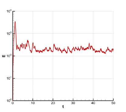
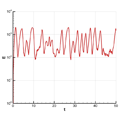
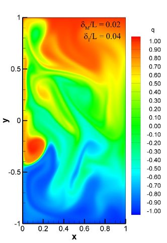
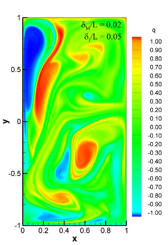
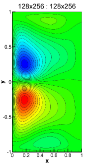
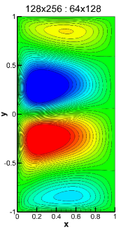
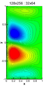
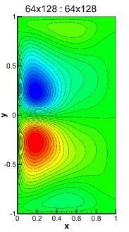
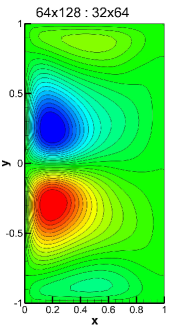
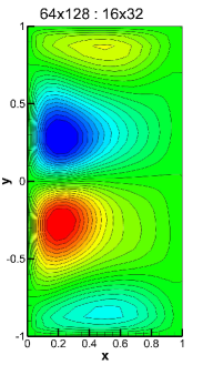
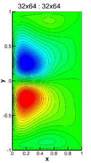
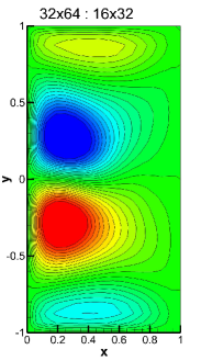
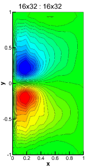
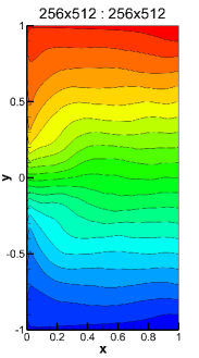
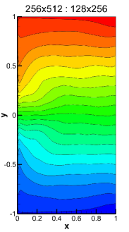

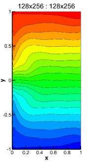
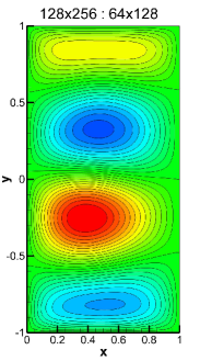
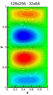
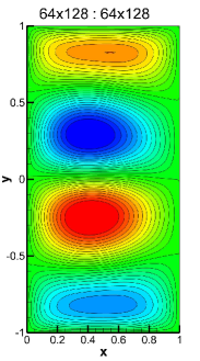
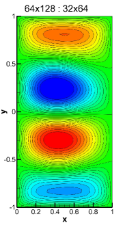

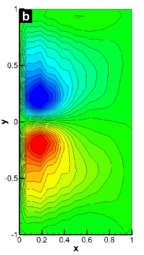
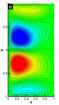
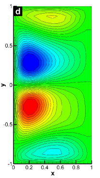
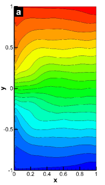
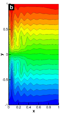
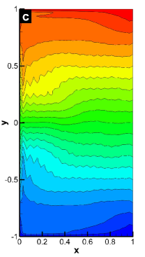

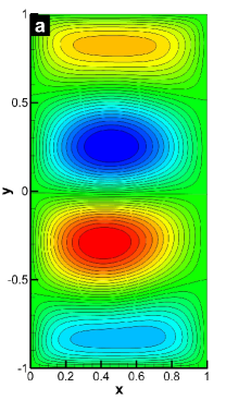
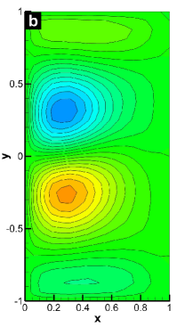
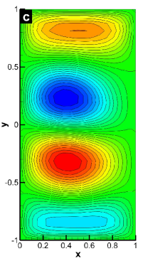
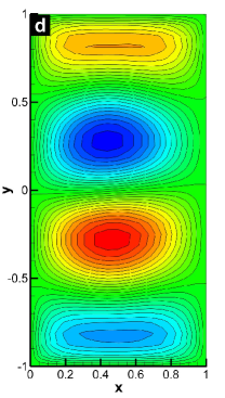
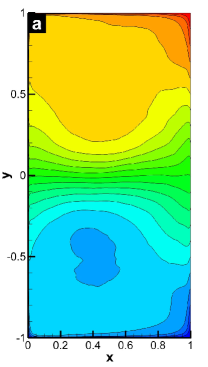
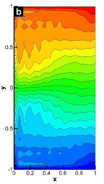
We start by performing a DNS computation on a fine mesh with a spatial resolution of . As shown in Fig. (2), for both experiments, after a transient period, a statistically steady state solution is obtained at a time of around . However, the behavior of the system in statistically steady state is quite different due to regime transition. In the classification of Berloff and McWilliams (1999), Experiment I lie in the chaotic regime, whereas in the Experiment II the flow regime showed a quasi-periodic variability. Instantaneous contour plots at the final time for the potential vorticity are shown in Fig. (3) for both experiments. In all the one-layer experiments presented in this study, the time average of the data is taken between time and using thousands snapshots in order to quantify the statistically steady state. The DNS results are included as a reference value in the following analysis when we present the results with the CGP method.
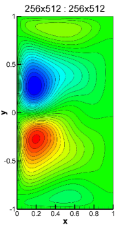
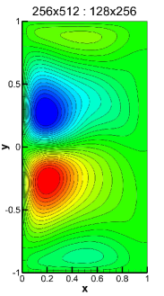
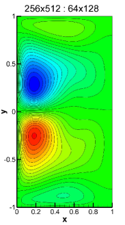
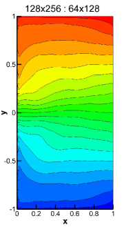
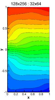
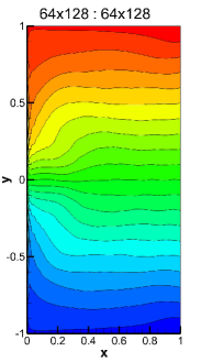
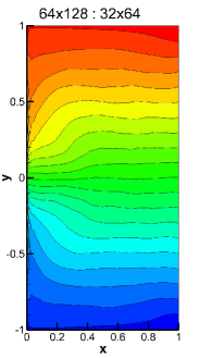
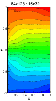
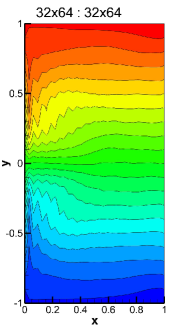
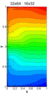
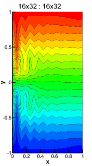
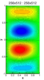
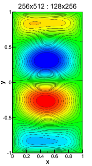
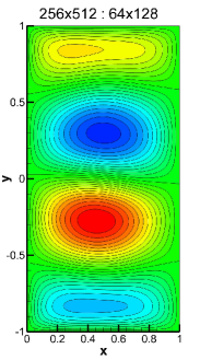
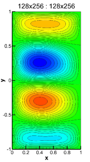
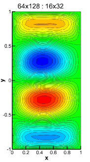
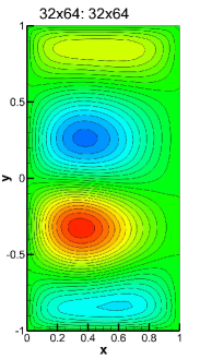
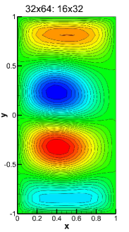
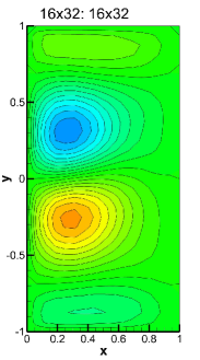
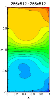
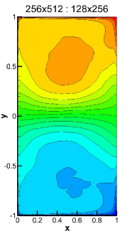
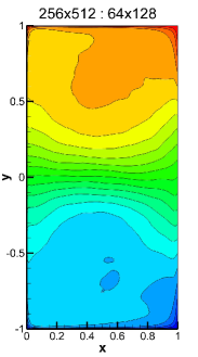
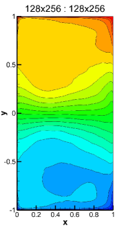
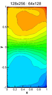
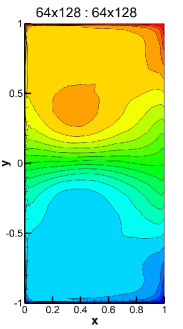
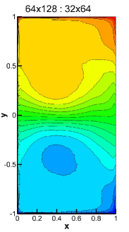
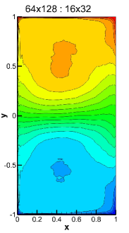
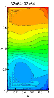
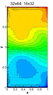
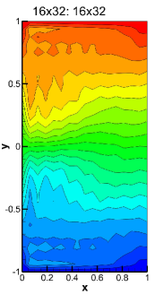
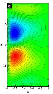
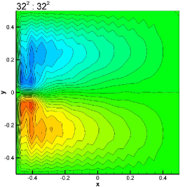
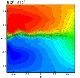
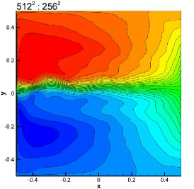
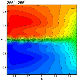
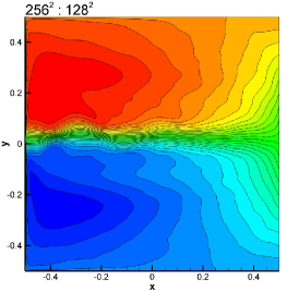
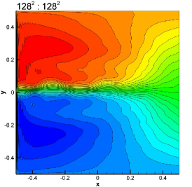
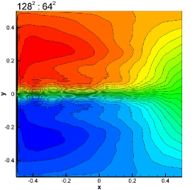
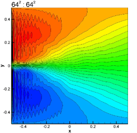
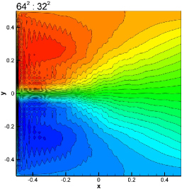
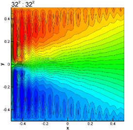
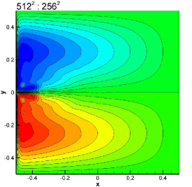
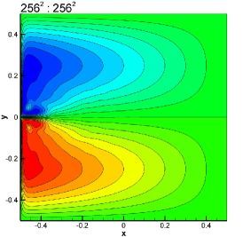
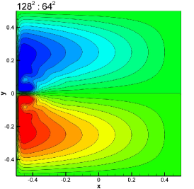
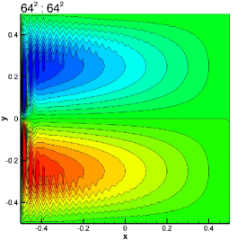
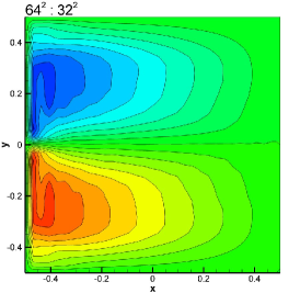
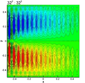
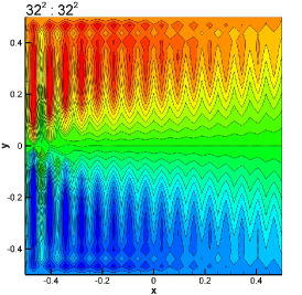
Three different levels of coarsening: half-coarsening (, ), -coarsening (, ) and -coarsening (, ), are performed to investigate the behavior of the CGP method. Mean stream function and potential vorticity field contours obtained using the CGP method are plotted in Fig. (4) and Fig. (5) along with the regular fine and coarse computations. In these figures, the labels show the resolutions in the form of , where is the resolution for the time dependant potential vorticity equation, and is the resolution for the elliptic sub-problem. The computed results with one level of coarsening are very close to those from the fine scale computations. Furthermore, results with two and three levels of coarsening also agree well with the fine scale computations. These results demonstrate that high fidelity numerical simulations can be obtained using the CGP method. For example, if we consider two numerical experiments with and resolutions, they have almost the same resulting flow field, but the latter results (with a half-coarsened grid for the elliptic sub-problem) were obtained almost 3 times faster than the former results (without CGP), and more importantly, the resulting field obtained using the CGP method with the resolution are better than those obtained on the grid without the CGP method.
Similar analysis is performed for the physical setting for Experiment II which shows a quasi-periodic flow regime. Comparisons of mean stream function and potential vorticity fields are plotted in Fig. (6) and Fig. (7), respectively. Similar to previous analysis, it is clear from these figures that the results using the CGP method agree well with the results of the fine scale computations using the standard method with a considerable reduction in computational cost. We emphasize that, for both parameter sets, four gyres are clearly visible in the stream function plots. It is more clear in Experiment II due to higher variability in quasi statistically steady state. These results demonstrate that the CGP methodology can provide an accelerated method for solving large scale QG models for ocean circulation problem.
In order to elucidate the fidelity of the CGP method for coarser resolutions, for Experiment I, we plot the time-averaged stream function and potential vorticity contours in Fig. (8) and Fig. (9), respectively. We include the high-resolution DNS results as well. In these figures, all results except the DNS are obtained with a constant resolution of for the elliptic sub-problem. One and two level coarsening methods are compared with non-coarsening standard procedure. We note that the new CGP models with both one-level and two-level coarsening yield improved results by smoothing out the numerical oscillations present in the results obtained by under-resolved standard computations without CGP method. This improvement is more clearly displayed in the potential vorticity contour plot in Fig. (9). Similar observations can be drawn from Fig. (10) and Fig. (11) for Experiment II. The CGP model yields results that are significantly better than those corresponding to the under-resolved BVE simulations having the same resolution for the elliptic sub-problem. In computational point of view, the price of CGP simulations are close to the price of the coarse grid simulation (i.e., the price of mapping operators and explicit time integration procedure is smaller than the price of solving elliptic sub-problem), while giving the same results as the high-resolution computations. In these computations we use a linear-cost fast Poisson solver, which is indeed one of the fastest elliptic solvers, and the CGP method yields a 3-8 fold reduction in computational cost. As discussed earlier, we highlight that the speed ups would be greater if we used a quadratic-cost sub-optimal elliptic solver.
5.2 CGP experiments for two-layer QG model
The main goal of this section is to test the CGP method in the numerical simulation of the two-layer QG model, which is a standard prototype representing many characteristics of more realistic ocean dynamics including stratification and baroclinic effects. To evaluate the performance of CGP method, we utilize two different parameter sets, corresponding to two physical oceanic settings: (i) Experiment 1 represents a moderate ocean basin with the physical parameters used by Özgökmen and Chassignet (1998), (ii) Experiment 2 represents a large ocean basin with the physical parameters used by Tanaka and Akitomo (2010). In terms of the classification given by Berloff and McWilliams (1999), both sets of experiments lie under the chaotic regime. The physical parameters and corresponding dimensionless parameters are summarized in Table 2.
| Variable (unit) | Experiment 1 | Experiment 2 |
|---|---|---|
| () | 2000 | 5000 |
| () | 1.0 | 0.6 |
| () | 4.0 | 3.4 |
| () | ||
| () | ||
| () | 1030 | 1030 |
| () | 0.02 | 0.02 |
| () | 0.1 | 0.1 |
| () | ||
| () | 50 | 100 |
| () | 14.19 | 17.88 |
| () | 2.86 | 22.86 |
| () | 31.56 | 25.77 |
| () | 42.79 | 31.16 |
| () | 0.0174 | 0.0116 |
| () | 3.64 | 13.64 |
| Ro | ||
| Fr | 0.087 | 0.073 |
| 0.2 | 0.15 | |
| Re | 697.16 | 580.97 |
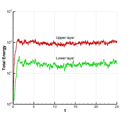
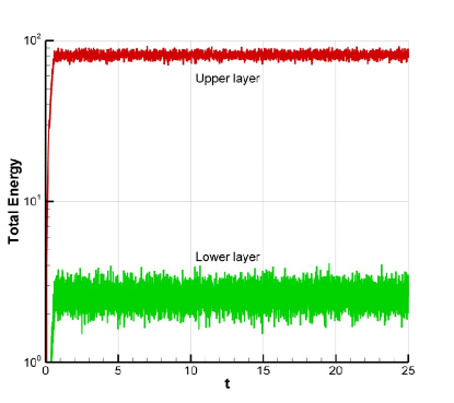







We start by performing a DNS on a fine mesh of spatial resolution. Similar to the one-layer analysis, we emphasize that the term DNS in this study is not meant to indicate that a fully detailed solution is being computed on the molecular viscosity scale, but instead refers to resolving the simulation down to the Munk scale via the specified lateral eddy viscosity parameterization. A statistically steady state solution is obtained after an initial transient spin-up process. The basin integrated total kinetic energy is
| (63) |
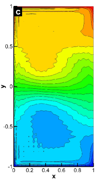
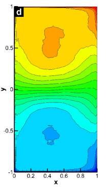
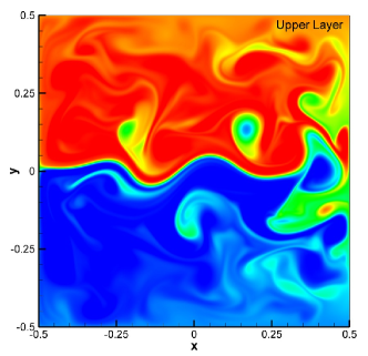
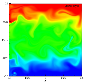
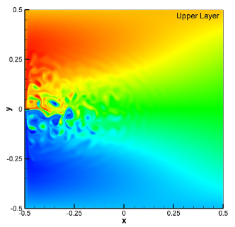
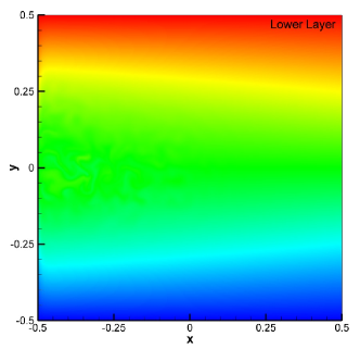
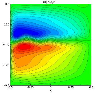
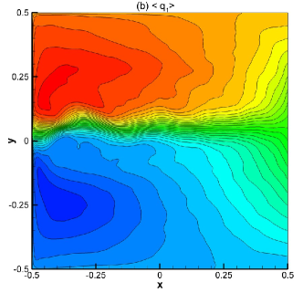
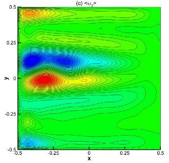
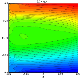
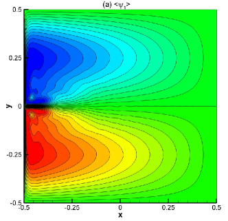
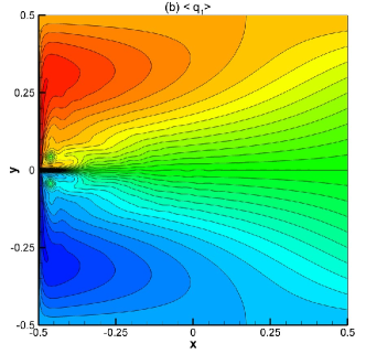
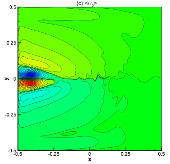
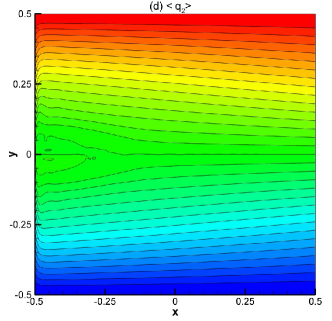
where the subscript represents the layer index. Figure 12 shows the time history of the basin integrated kinetic energy for the upper and lower layers for both of the oceanic settings. As shown in this figure, the system reaches the statistically steady state after the dimensionless time . As expected, the total energy of the upper layer is much larger than that in the lower layer. It is important to emphasize that, second layer in Experiment 1 is more active than that of Experiment 2. Instantaneous contour plots for the potential vorticities in the upper and lower layers are shown in Figure 13 and Figure 14 for Experiment 1 and Experiment 2, respectively. The length scales in these two experiments are quite different. For example, the ratio of the basin length scale to the Rossby deformation radius is for Experiment 1 and for Experiment 2. Therefore, the structure of the eastward jet formation on the western boundary for Experiment 1 is different from that of Experiment 2. This difference becomes more obvious in the mean flow field. The results for time-averaged mean field data obtained from thousands snapshots between time and in the statistically steady state are given in Figure 15 and Figure 16. The results show strong western boundary currents with cyclonic (counter-clockwise rotating) subpolar gyres and anticyclonic (clockwise rotating) subtropical gyres producing a strong eastward jet in both experiments. However, the produced eastward jet formation in Experiment 1 shows swirling structure and almost reaches the eastern boundary of the basin. Compared to Experiment 2, the bottom layer is more active in Experiment 1. Since in Experiment 1 we used the same parameters and boundary conditions as in Özgökmen and Chassignet (1998), the plot in Figure 15 is similar to Figure 2 in Özgökmen and Chassignet (1998). Although in Experiment 2 we have used the same parameters as those used in Tanaka and Akitomo (2010), the boundary conditions we used are different from their boundary conditions: we used the slip boundary conditions, whereas they used the no-slip boundary conditions. Thus, the plot in Figure 16 is different from the corresponding one in Tanaka and Akitomo (2010).
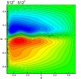
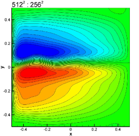
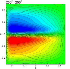
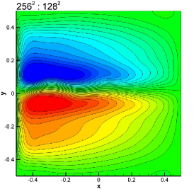
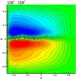
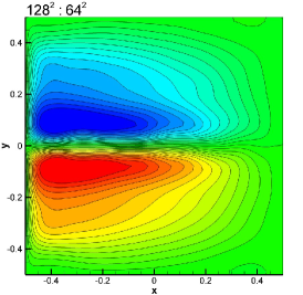
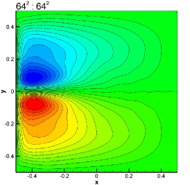
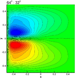
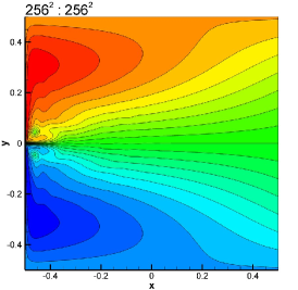
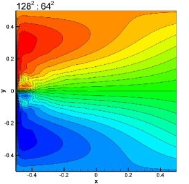
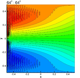
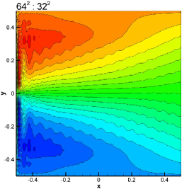
To test the CGP method, we employ the standard coarsening methodology. The criterion used in assessing the success of the new CGP model is its ability to produce more accurate (i.e., closer to the DNS) results than those for standard method without CGP having the same resolution for elliptic sub-problem, without a significant increase in computational time. For Experiment 1, we plot the mean stream function and potential vorticity contours in Figs. (17) and (18), respectively. The various resolutions used in the computations are written in the labels of the subfigures. The labels include the resolution for the time dependant part and the resolution for the elliptic part, as described in the captions. As was the case in previous analysis for one-layer model, we compare the CGP computations with standard computations without CGP. For example, the flow field obtained by a standard computation with agrees well with that obtained by the CGP method with , and better than that of the standard computation with . Similar observations holds for higher and lower resolution computations as well. It can clearly be seen that the CGP approach provides results at the same level of accuracy, but at a reduced computational cost compared to the standard, fine-resolution simulations, by reducing the resolution of the elliptic sub-problem.
Similarly, we plot the mean stream function and potential vorticity contours in Figs. (19) and (20) for Experiment 2. We note that the proposed CGP model yields again improved results by smoothing out the numerical oscillations present in the under-resolved standard simulations without CGP. The numerical results for both experiments clearly suggest that the the CGP model can provide relatively accurate results for stratified geophysical flows at a low computational cost.
6 Conclusions
A new coarse grid projection (CGP) multiscale method was introduced for large-scale ocean circulation models. The CGP method was tested in the numerical simulation of the wind-driven circulation in both one-layer and two-layer ocean basins, standard prototypes of more realistic ocean dynamics. The first mathematical model employed was the barotropic vorticity equation (BVE) for the one-layer quasigeostropic model, which is driven by a symmetric double-gyre wind forcing that yielded a four-gyre circulation in the time mean. The second mathematical model used was the two-layer quasigeostropic equations for a stratified ocean model accounting for baroclinic effects.
In the CGP methodology the cost of large-scale ocean dynamics computations is reduced by coarsening the number of grid points used for the solution of the elliptic sub-problem in quasigeostropic (QG) ocean models. The CGP approach is general and in fact constitutes a family of methods, since in addition to choosing the coarsening and prolongation operators and the time integration scheme, the elliptic solver used in the approach can vary. In this work, we investigated the performance of a particular CGP method that uses an optimal FFT based elliptic solver, the full weighting operation for the coarsening operator, and bilinear interpolation for the prolongation operator. We used the spatially second-order accurate fully conservative Arakawa scheme along with the third-order TVD Runge-Kutta time integration scheme. The CGP method was tested on meshes that were coarser than those used for the direct numerical simulation (DNS) computations. The CGP method yielded numerical results that were in close agreement with those of the DNS for both barotropic and stratified ocean circulation models. In particular, we found that the new CGP models with both one-level and multiple-level coarsening yield improved results by smoothing out the numerical oscillations present in the results obtained by under-resolved standard computations without the CGP procedure. This first step in the numerical assessment of the proposed ocean circulation models shows that CGP methodology could represent a viable tool for QG models of more realistic turbulent geophysical flows.
Acknowledgements
This research was partially supported by the Institute for Critical Technology and Applied Science (ICTAS) at Virginia Tech via grant number 118709.
References
- Alam (2011) Alam, J.M. Towards a multiscale approach for computational atmospheric modelling. Mon. Wea. Rev., 139:3906 –3922, 2011.
- Allen (1980) Allen, J.S. Models of wind-driven currents on the continental shelf. Annu. Rev. Fluid Mech., 12:389–433, 1980.
- Arakawa (1966) Arakawa, A. Computational design for long-term numerical integration of the equations of fluid motion: Two-dimensional incompressible flow. Part I. J. Comput. Phys., 1:119–143, 1966.
- Barth et al. (2002) Barth, T.J.; Chan, T.F., and Haimes, R. Multiscale and multiresolution methods: Theory and applications. Springer Verlag, 2002.
- Berloff et al. (2009) Berloff, P.; Kamenkovich, I., and Pedlosky, J. A mechanism of formation of multiple zonal jets in the oceans. J. Fluid Mech., 628:395–425, 2009.
- Berloff and McWilliams (1999) Berloff, P.S. and McWilliams, J.C. Large-scale, low-frequency variability in wind-driven ocean gyres. J. Phys. Oceanogr., 29:1925–1949, 1999.
- Berselli et al. (2006) Berselli, L.C.; Iliescu, T., and Layton, W.J. Mathematics of large eddy simulation of turbulent flows. Springer Verlag, 2006.
- Brandt (1977) Brandt, A. Multi-level adaptive solutions to boundary value problems. Math. Comp., 31:333–390, 1977.
- Brandt (2002) Brandt, A. Multiscale scientific computation: Review 2001. In Barth, T.J.; Chan, T., and Haimes, R., editors, Lecture Notes in Computational Science and Engineering, volume 20, pages 3–96. Springer Verlag, Heidelberg, 2002.
- Brandt (2005) Brandt, A. Multiscale solvers and systematic upscaling in computational physics. Comp. Phys. Commun., 169:438–441, 2005.
- Brandt (2010) Brandt, A. Principles of systematic upscaling. In Multiscale methods: Bridging the scales in science and engineering, pages 193–215. Oxford University Press, New York, 2010.
- Brezina et al. (2005) Brezina, M.; Falgout, R.; MacLachlan, S.; Manteuffel, T.; McCormick, S., and Ruge, J. Adaptive smoothed aggregation (sa) multigrid. SIAM Rev., pages 317–346, 2005.
- Briggs et al. (2000) Briggs, W.L.; Henson, V.E., and McCormick, S.F. A multigrid tutorial. Society for Industrial Mathematics, 2000.
- Bryan (1963) Bryan, K. A numerical investigation of a nonlinear model of a wind-driven ocean. J. Atmos. Sci., 20:594–606, 1963.
- Campin et al. (2011) Campin, J.M.; Hill, C.; Jones, H., and Marshall, J. Super-parameterization in ocean modeling: Application to deep convection. Ocean Modell., 36:90–101, 2011.
- Chang et al. (2001) Chang, K.I.; Ghil, M.; Ide, K., and Lai, C.C.A. Transition to aperiodic variability in a wind-driven double-gyre circulation model. J. Phys. Oceanogr., 31:1260–1286, 2001.
- Cummins (1992) Cummins, P.F. Inertial gyres in decaying and forced geostrophic turbulence. J. Mar. Res., 50:545–566, 1992.
- DiBattista and Majda (2001) DiBattista, M.T. and Majda, A.J. Equilibrium statistical predictions for baroclinic vortices: The role of angular momentum. Theor. Comp. Fluid Dyn., 14:293–322, 2001.
- Dijkstra (2005) Dijkstra, H.A. Nonlinear physical oceanography. Springer, 2005.
- Dijkstra and Ghil (2005) Dijkstra, H.A. and Ghil, M. Low-frequency variability of the large-scale ocean circulation: A dynamical systems approach. Rev. Geophys., 43:122–59, 2005.
- E (2011) E, W. Principles of Multiscale Modeling. Cambridge University Press, 2011.
- E et al. (2007) E, W.; Engquist, B.; Li, X.; Ren, W., and Vanden-Eijnden, E. The heterogeneous multiscale method: A review. Commun. Comput. Phys., 2:367–450, 2007.
- Fish (2009) Fish, J. Multiscale methods: Bridging the scales in science and engineering. Oxford University Press, USA, 2009.
- Fish and Chen (2004) Fish, J. and Chen, W. Discrete-to-continuum bridging based on multigrid principles. Comput. Methods Appl. Mech. Engrg., 193:1693–1711, 2004.
- Fox-Kemper (2005) Fox-Kemper, B. Reevaluating the roles of eddies in multiple barotropic wind-driven gyres. J. Phys. Oceanogr., 35:1263–1278, 2005.
- Ghil et al. (2008) Ghil, M.; Chekroun, M.D., and Simonnet, E. Climate dynamics and fluid mechanics: Natural variability and related uncertainties. Physica D, 237:2111–2126, 2008.
- Gottlieb and Shu (1998) Gottlieb, S. and Shu, C.W. Total variation diminishing Runge-Kutta schemes. Math. Comput., 67:73–85, 1998.
- Greatbatch and Nadiga (2000) Greatbatch, R.J. and Nadiga, BT. Four-gyre circulation in a barotropic model with double-gyre wind forcing. J. Phys. Oceanogr., 30:1461–1471, 2000.
- Griffa and Salmon (1989) Griffa, A. and Salmon, R. Wind-driven ocean circulation and equilibrium statistical mechanics. J. Mar. Res., 47:457–492, 1989.
- Gupta et al. (1997) Gupta, M.M.; Kouatchou, J., and Zhang, J. Comparison of second-and fourth-order discretizations for multigrid Poisson solvers. J. Comput. Phys., 132:226–232, 1997.
- Hackbusch (1985) Hackbusch, W. Multi-grid methods and applications. Springer Verlag, 1985.
- Holland (1978) Holland, W.R. The role of mesoscale eddies in the general circulation of the ocean-numerical experiments using a wind-driven quasi-geostrophic model. J. Phys. Oceanogr., 8:363–392, 1978.
- Holland and Rhines (1980) Holland, W.R. and Rhines, P.B. An example of eddy-induced ocean circulation. J. Phys. Oceanogr., 10:1010–1031, 1980.
- Höllig et al. (2002) Höllig, K.; Reif, U., and Wipper, J. Multigrid methods with web-splines. Numer. Math., 91:237–256, 2002.
- Holm and Nadiga (2003) Holm, D.D. and Nadiga, B.T. Modeling mesoscale turbulence in the barotropic double-gyre circulation. J. Phys. Oceanogr., 33:2355–2365, 2003.
- Hurrell et al. (2009) Hurrell, J.; Meehl, G.A.; Bader, D.; Delworth, T.L.; Kirtman, B., and Wielicki, B. A unified modeling approach to climate system prediction. B. Am. Meteorol. Soc., 90(12):1819, 2009.
- Iskandarani et al. (2002) Iskandarani, M.; Haidvogel, D.B.; Levin, J.C.; Curchitser, E., and Edwards, C.A. Multi-scale geophysical modeling using the spectral element method. Comput. Sci. Eng., 4:42–48, 2002.
- Kelly et al. (2010) Kelly, K.A.; Small, R.J.; Samelson, R.M.; Qiu, B.; Joyce, T.M.; Kwon, Y.O., and Cronin, M.F. Western boundary currents and frontal air-sea interaction: Gulf stream and kuroshio extension. J. Climate, 23:5644–5667, 2010.
- Kevrekidis and Samaey (2009) Kevrekidis, I.G. and Samaey, G. Equation-free multiscale computation: Algorithms and applications. Annu. Rev. Phys. Chem., 60:321–344, 2009.
- Khairoutdinov et al. (2008) Khairoutdinov, M.; DeMott, C., and Randall, D. Evaluation of the simulated interannual and subseasonal variability in an amip-style simulation using the csu multiscale modeling framework. J. Climate, 21(3):413–431, 2008.
- Klein (2010) Klein, R. Scale-dependent models for atmospheric flows. Annu. Rev. Fluid Mech., 42:249–274, 2010.
- Lee et al. (1997) Lee, S.; Wolberg, G., and Shin, S.Y. Scattered data interpolation with multilevel b-splines. IEEE T. Vis. Comput. Gr., 3:228–244, 1997.
- Lentine et al. (2010) Lentine, M.; Zheng, W., and Fedkiw, R. A novel algorithm for incompressible flow using only a coarse grid projection. ACM T. Graphic., 29:114:1–9, 2010.
- Lynch (2008) Lynch, P. The origins of computer weather prediction and climate modeling. J. Comput. Phys., 227:3431–3444, 2008.
- Majda and Wang (2006) Majda, A. and Wang, X. Non-linear dynamics and statistical theories for basic geophysical flows. Cambridge University Press, 2006.
- Majda and Klein (2003) Majda, A.J. and Klein, R. Systematic multiscale models for the tropics. J. Atmos. Sci., 60:393–408, 2003.
- Marshall et al. (1997) Marshall, J.; Hill, C.; Perelman, L., and Adcroft, A. Hydrostatic, quasi-hydrostatic, and nonhydrostatic ocean modeling. J. Geophys. Res., 102:5733–5752, 1997.
- McWilliams (2006) McWilliams, J.C. Fundamentals of geophysical fluid dynamics. Cambridge University Press, 2006.
- Meacham (2000) Meacham, S.P. Low-frequency variability in the wind-driven circulation. J. Phys. Oceanogr., 30:269–293, 2000.
- Medjo (2000) Medjo, T.T. Numerical simulations of a two-layer quasi-geostrophic equation of the ocean. SIAM J. Numer. Anal., 37:2005–2022, 2000.
- Miller (2007) Miller, R.N. Numerical modeling of ocean circulation. Cambridge University Press, 2007.
- Moin (2001) Moin, P. Fundamentals of engineering numerical analysis. Cambridge University Press, 2001.
- Munk and Wunsch (1982) Munk, W. and Wunsch, C. Observing the ocean in the 1990s. Phil. Trans. R. Soc. Lond. A, 307:439–464, 1982.
- Munk (1950) Munk, W.H. On the wind-driven ocean circulation. J. Meteor., 7:80–93, 1950.
- Nadiga and Margolin (2001) Nadiga, B.T. and Margolin, L.G. Dispersive-dissipative eddy parameterization in a barotropic model. J. Phys. Oceanogr., 31:2525–2531, 2001.
- Nauw et al. (2004) Nauw, J.J.; Dijkstra, H.A., and Simonnet, E. Regimes of low-frequency variability in a three-layer quasi-geostrophic ocean model. J. Mar. Res., 62:684–719, 2004.
- Özgökmen and Chassignet (1998) Özgökmen, T.M. and Chassignet, E.P. Emergence of inertial gyres in a two-layer quasigeostrophic ocean model. J. Phys. Oceanogr., 28:461–484, 1998.
- Özgökmen et al. (2001) Özgökmen, T.M.; Chassignet, E.P., and Rooth, C.G.H. On the connection between the Mediterranean outflow and the Azores Current. J. Phys. Oceanogr., 31:461–480, 2001.
- Pedlosky (1987) Pedlosky, J. Geophysical fluid dynamics. Springer, 1987.
- Press et al. (1992) Press, W.H.; Teukolsky, S.A.; Vetterling, W.T., and Flannery, B.P. Numerical recipes in FORTRAN: The art of scientific computing. Cambridge Univ Press, 1992.
- Ringler et al. (2011) Ringler, T.D.; Jacobsen, D.; Gunzburger, M.; Ju, L.; Duda, M., and Skamarock, W. Exploring a multi-resolution modeling approach within the shallow-water equations. Mon. Wea. Rev., 139:3348 –3368, 2011.
- Saad (2003) Saad, Y. Iterative methods for sparse linear systems. Society for Industrial and Applied Mathematics, 2003.
- Sagaut (2006) Sagaut, P. Large eddy simulation for incompressible flows: An introduction. Springer Verlag, 2006.
- Salmon (1998) Salmon, R. Lectures on geophysical fluid dynamics. Oxford University Press, 1998.
- San and Staples (2012) San, O. and Staples, A. E. A coarse-grid projection method for accelerating incompressible flow computations. J. Comput. Phys., 233:480–508, 2013.
- San et al. (2011) San, O.; Staples, A. E.; Wang, Z., and Iliescu, T. Approximate deconvolution large eddy simulation of a barotropic ocean circulation model. Ocean Modell., 40:120–132, 2011.
- Schäfer (2006) Schäfer, M. Computational engineering: Introduction to numerical methods. Springer Verlag, 2006.
- Siegel et al. (2001) Siegel, A.; Weiss, J.B.; Toomre, J.; McWilliams, J.C.; Berloff, P.S., and Yavneh, I. Eddies and vortices in ocean basin dynamics. Geophys. Res. Lett., 28:3183–3186, 2001.
- Speich et al. (1995) Speich, S.; Dijkstra, H., and Ghil, M. Successive bifurcations in a shallow-water model applied to the wind-driven ocean circulation. Nonlinear Proc. Geoph., 2:241–268, 1995.
- Stocker (2011) Stocker, T. Introduction to Climate Modelling. Springer Verlag, Heidelberg, 2011.
- Stommel (1972) Stommel, H. The Gulf Stream: A physical and dynamical description. University of California Press, 1972.
- Tanaka and Akitomo (2010) Tanaka, Y. and Akitomo, K. Alternating zonal flows in a two-layer wind-driven ocean. J. Oceanogr., 66:475–487, 2010.
- Trottenberg et al. (2001) Trottenberg, U.; Oosterlee, C.W., and Schüller, A. Multigrid. Academic Press, London, 2001.
- Vallis (2006) Vallis, G.K. Atmospheric and oceanic fluid dynamics: fundamentals and large-scale circulation. Cambridge University Press, 2006.
- Wagner et al. (2010) Wagner, G.J.; Zhou, X., and Plimpton, S.J. Equation-free accelerated simulations of the morphological relaxation of crystal surfaces. Int. J. Mult. Comp. Eng., 8:423–439, 2010.
- Wesseling (2004) Wesseling, P. Introduction to multigrid methods. R.T. Edwards, Inc., 2004.
- Zhang (1998) Zhang, J. Fast and high accuracy multigrid solution of the three dimensional Poisson equation. J. Comput. Phys., 143:449–461, 1998.