Double-dimers, the Ising model and the hexahedron recurrence

Abstract

We define and study a recurrence relation in $\mathbb{Z}^{3}$, called the hexahedron recurrence, which is similar to the octahedron recurrence (Hirota bilinear difference equation) and cube recurrence (Miwa equation). Like these examples, solutions to the hexahedron recurrence are partition sums for edge configurations on a certain graph, and have a natural interpretation in terms of cluster algebras. We give an explicit correspondence between monomials in the Laurent expansions arising in the recurrence with certain double-dimer configurations of a graph. We compute limit shapes for the corresponding double-dimer configurations.

The Kashaev difference equation arising in the Ising model star-triangle relation is a special case of the hexahedron recurrence. In particular this reveals the cluster nature underlying the Ising model. The above relation allows us to prove a Laurent phenomenon for the Kashaev difference equation.

1 Introduction

1.1 Overview

A function $a:\mathbb{Z}^{3}\to\mathbb{C}$ is said to satisfy the octahedron recurrence or Hirota bilinear difference equation if at all points $v\in\mathbb{Z}^{3}$

$$a_{(1)}a_{(23)}=a_{(2)}a_{(13)}+a_{(3)}a_{(12)}$$ (1)

(here $a_{(S)}\equiv a_{v+(S)}$ represents $a$ evaluated at the translate of $v$ by the basis vectors in $S$, e.g. $a_{(12)}$ represents $a_{v+e_{1}+e_{2}}$). The octahedron recurrence was coined by Propp (see [19]) but first appeared in Dodgson [5] as a means of recursively computing determinants: up to an affine change of indices (and some sign changes) it is the recurrence satisfied by determinants of contiguous submatrices. In this setting it is known as Dodgson condensation.

The octahedron recurrence is fundamental in combinatorics, statistical mechanics, cluster algebras, and integrable systems, see e.g. [15].

There are several similar recurrences. The most well-known is the cube recurrence or Miwa equation. A function $g:\mathbb{Z}^{3}\to\mathbb{C}$ is said to satisfy the Miwa equation or cube recurrence if

$$g_{(123)}g=g_{(1)}g_{(23)}+g_{(2)}g_{(13)}+g_{(3)}g_{(12)}.$$ (2)

This recurrence also has its roots in the $19^{th}$ century: Kennelly [12] discovered the so-called star-triangle identity (wye-delta transformation) for resistor networks. Under a certain change of variables (see [8, 9]) this transformation can be written as a cube recurrence.

In [8], see also [9], it was noticed that the cube recurrence is a specialization of a more fundamental recurrence, which we call the cuboctahedron recurrence. This is a recurrence on a function on the edges of the cubes of the $\mathbb{Z}^{3}$ lattice. If certain monomial equations are satisfied then the cuboctahedron recurrence reduces to the cube recurrence. Like the octahedron recurrence, the cuboctahedron recurrence arises from cluster algebras, and in fact is a composition of cluster algebra mutations on a certain planar graph. This leads to a cluster algebra interpretation of the cube recurrence, and in particular allows one to prove a Laurent phenomenon as shown in [8].

A less-well known recurrence is the Kashaev recurrence [11]. A function $f:\mathbb{Z}^{3}\to\mathbb{C}$ is said to satisfy the Kashaev recurrence if

$$f^{2}f_{(123)}^{2}+f_{(1)}^{2}f_{(23)}^{2}+f_{(2)}^{2}f_{(13)}^{2}+f_{(3)}^{2}f_{(12)}^{2}-2f_{(1)}f_{(2)}f_{(23)}f_{(13)}-2f_{(1)}f_{(3)}f_{(23)}f_{(12)}-2f_{(3)}f_{(2)}f_{(12)}f_{(13)}$$ (3)

$$-2ff_{(123)}(f_{(1)}f_{(23)}+f_{(2)}f_{(13)}+f_{(3)}f_{(12)})-4ff_{(23)}f_{(13)}f_{(12)}-4f_{(123)}f_{(1)}f_{(2)}f_{(3)} = 0.$$

This recurrence arises in the star-triangle move (Yang-Baxter equation) for the Ising model.

Our main goal in this paper is to define another recurrence, generalizing the Kashaev recurrence, called the hexahedron recurrence. This is a relation for a function defined on the faces and vertices of the $\mathbb{Z}^{3}$ cubic tiling. Given four functions

$$h,h^{(x)},h^{(y)},h^{(z)}\colon\mathbb{Z}^{3}\to\mathbb{C}$$

(where we think of $h$ as being the function on the vertices of the cubes, $h^{(x)}_{v}$ as being the value of the function on the “yz”-face with vertices $\{v,v+e_{2},v+e_{2}+e_{3},v+e_{3}\}$, and similarly for $h_{v}^{(y)}$ and $h_{v}^{(z)}$ on the “xz” and “xy” faces respectively) we say they satisfy the hexahedron recurrence if the following equations are satisfied for all $v\in\mathbb{Z}^{3}$.

$$h^{(x)}_{(1)}h^{(x)}h = h^{(x)}h^{(y)}h^{(z)}+h_{(1)}h_{(2)}h_{(3)}+hh_{(1)}h_{(23)}$$ (4)

$$h^{(y)}_{(2)}h^{(y)}h = h^{(x)}h^{(y)}h^{(z)}+h_{(1)}h_{(2)}h_{(3)}+hh_{(2)}h_{(13)}$$ (5)

$$h^{(z)}_{(3)}h^{(z)}h = h^{(x)}h^{(y)}h^{(z)}+h_{(1)}h_{(2)}h_{(3)}+hh_{(3)}h_{(12)}$$ (6)

$$h_{(123)}h^{2}h^{(x)}h^{(y)}h^{(z)} = (h^{(x)}h^{(y)}h^{(z)})^{2}+h^{(x)}h^{(y)}h^{(z)}(2h_{(1)}h_{(2)}h_{(3)}+hh_{(1)}h_{(23)}+hh_{(2)}h_{(13)}+hh_{(3)}h_{(12)})+$$ (7)

$$+(h_{(1)}h_{(2)}+hh_{(12)})(h_{(1)}h_{(3)}+hh_{(13)})(h_{(2)}h_{(3)}+hh_{(23)}).$$

Here again $h_{(1)}=h_{v+e_{1}}$ and so on. In Section 6 below we will show that the Kashaev recurrence is a special case of the hexahedron recurrence. Understanding the cluster algebra structure of the Y-Delta transformation for the Ising model was our initial motivation for defining the hexahedron recurrence.

The octahedron, cuboctahedron and hexahedron recurrences have an underlying cluster algebra structure, based on the local transformation (mutation) called urban renewal, see Figure 3. For example the octahedron recurrence can be thought of as a “periodic” urban renewal step on the square grid graph; the cuboctahedron recurrence can be decomposed into a product of $4$ periodic urban renewal steps, see [8]. The hexahedron recurrence can be decomposed into a product of $6$ periodic urban renewals. In particular this allows us to write $h_{i,j,k},h^{(x)}_{i,j,k},h^{(y)}_{i,j,k},h^{(z)}_{i,j,k}$ for $i+j+k$ large as Laurent polynomials in the initial values $\{h_{i,j,k}\}_{0\leq i+j+k\leq 2}$ and $\{h^{(x)}_{i,j,k},h^{(y)}_{i,j,k},h^{(z)}_{i,j,k}\}_{i+j+k=0}$.

Speyer [19] and Carroll and Speyer [3] respectively gave combinatorial interpretations of the terms in the Laurent expansions arising in the octahedron and cube recurrences. One of our main results is an analogous result for the hexahedron recurrence: we give an explicit bijection between the monomials of the Laurent polynomials which arise and certain “taut” double-dimer covers of a sequence of planar graphs $\Gamma_{n}$.

Following the method of Peterson and Speyer [18] we also prove a limit shape theorem for random taut double-dimer covers of $\Gamma_{n}$ with an arctic boundary which is an algebraic curve defined from the characteristic polynomial of the recurrence relation.

The integrable nature of these systems will not be discussed here (although it is easy to show that they satisfy a standard multidimensional consistency). The hexahedron recurrence is a special case of a dimer integrable system, and integrable properties of such systems are discussed in [9].

1.2 Results

We may picture the values of $h^{(x)}$, $h^{(y)}$ and $h^{(z)}$ as each sitting in the middle of a square face of the integer lattice. Letting

$${\mathbb{Z}^{3}_{1/2}}:=\{(x,y,z)\in(1/2)\mathbb{Z}^{3}:x+y+z\in\mathbb{Z}\}$$

we then interpret $h^{(x)},h^{(y)},h^{(z)}$ as extending $h$ to ${\mathbb{Z}^{3}_{1/2}}$ via $h^{(x)}(i,j,k)=h(i,j+1/2,k+1/2)$, $h^{(y)}(i,j,k)=h(i+1/2,j,k+1/2)$, and $h^{(z)}(i,j,k)=h(i+1/2,j+1/2,k)$.

Note that the equations (4-7) are not only homogeneous, but are 1-homogeneous: the sum of all indices of each monomial is $3$, e.g., the first monomial is the product of three variables with respective indices $(1,1/2,1/2)$, $(0,1/2,1/2)$ and $(0,0,0)$. Also, given the values of $h$ on seven of the corners and their three included faces of a cube, the values on the eighth corner and the three remaining faces are determined as rational functions of these; the locations of the new values are precisely those obtained if one increases a pile by a single cube.

The cluster nature of the hexahedron recurrence immediately implies:

Theorem.

The values $\{h(v):v\in{\mathbb{Z}^{3}_{1/2}},v_{1}+v_{2}+v_{3}\geq 0\}$ are Laurent polynomials in the values of $h(v)$ such that $v$ is an integer vector and $0\leq v_{1}+v_{2}+v_{3}\leq 2$ or $v$ is a half-integer vector and $v_{1}+v_{2}+v_{3}=1$.

Our main result, Theorem 4.1 below, gives a combinatorial interpretation of the terms of these Laurent polynomials.

1.3 Statistical mechanical interpretations

The octahedron recurrence may be used to express $a_{v}$ as a Laurent polynomial in the values $a_{w}$ as $w$ ranges over variables in an initial graph. When the initial graph is the grid $\mathbb{Z}^{2}$ this Laurent polynomial is a generating function for a certain statistical mechanical ensemble: its monomials are in bijection with perfect matchings of the Aztec diamond graph, associated with the region in the initial graph lying in the shadow of $v$; see, e.g., [19]. Setting the initial indeterminates all equal to one allows us to count perfect matchings; in general the indeterminates represent multiplicative weights, which we may change in certain natural ways to study further properties of the ensemble of perfect matchings. These ensembles, well studied on the square lattice, exist on many other periodic bipartite planar graphs.

The cube recurrence (2) also has a combinatorial interpretation. Its monomials are in bijection with cube groves. These were first defined and studied in [3, 18] where they were called simply “groves”. In a cube grove, each edge of a large triangular region in the planar triangular lattice is either present or absent. The allowed configurations are those in which the edge subsets contain no cycles and no islands (thus they are essential spanning forests), and the connectivity of boundary points has a prescribed form.

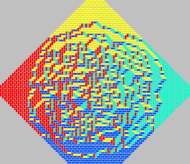
Both Aztec diamond matchings and cube groves have limiting shapes. Specifically, as the size of the box goes to infinity, there is a boundary, which is an algebraic curve, outside of which there is no entropy (the system is periodic almost surely) and inside of which there is positive entropy per site (each type of local configuration occurs with positive probability). In the case of the Aztec diamond and cube grove, the algebraic curve is the inscribed circle, but for related ensembles, much more general algebraic curves are obtained; for example in the fortress tiling model shown on the right of Figure 1, the bounding curve is a degree-8 algebraic curve, see [13].

Figure 1: An Aztec tiling, a cube grove and a fortress tiling

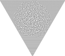
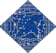
The hexahedron recurrence also has a statistical mechanical interpretation. In Section 2 we define the double-dimer model on a finite bipartite graph. Terms in the hexahedron recurrence count certain types of double-dimer configurations called taut configurations. A randomly generated taut double-dimer configuration is shown in Figure 2.

Figure 2: A random taut double-dimer configuration

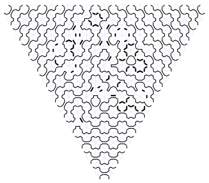
In Section 4 we prove the following theorem.

Theorem.

The monomials of the Laurent polynomial $h_{iii}$ are in bijection with taut double-dimer configurations of the graph $\Gamma_{3i}$.

The remainder of the paper is spent investigating the properties of the hexahedron double-dimer ensemble. In Section 5 we analyze the limiting shape under several natural, periodic specifications of the initial variables. In Section 6 we find a specialization of the initial variables under which the hexahedron recurrence becomes the Ising $Y$-$\Delta$ transformation.

Acknowledgements. We would like to thank Philippe Di Francesco, Sergei Fomin, David Speyer and Dylan Thurston for helpful discussions.

2 Dimer model

2.1 Definitions

We will use the following graph theoretic terminology. A bipartite graph is a graph $\Gamma=(E,V)$ together with a fixed coloring of the vertices into two colors (black and white) such that edges connect only vertices of different colors. By planar graph we mean one with a distinguished planar embedding. The dual graph $\Gamma_{*}$ to a planar bipartite graph $\Gamma$ has a vertex $f_{*}$ for each face $f$ of $\Gamma$ and edge $e_{*}$ connecting $f_{*}$ and $g_{*}$ where $f$ and $g$ are the two faces containing $e$.

Let $\Gamma$ be a finite bipartite graph with positive edge weights $\nu:E\to\mathbb{R}_{+}$. A dimer cover or perfect matching is a collection of edges with the property that every vertex is an endpoint of exactly one edge. The “dimers” of a dimer cover are the chosen edges (terminology suggesting a collection of bi-atomic molecules packed into the graph). We let $\Omega_{d}(\Gamma)$ be the set of dimer covers and we define the probability measure $\mu_{d}$ on $\Omega_{d}$ giving a dimer cover $m\in\Omega_{d}$ a probability proportional to the product of its edge weights.

A double-dimer configuration is a union of two dimer covers: it is a covering of the graph with loops and doubled edges. The double dimer measure $\mu_{dd}$ is the probability measure defined by taking the union of two $\mu_{d}$-independent dimer covers.

2.2 Edge variables, face variables, and cluster variables

2.2.1 Gauge transformations

A gauge transformation consists in multiplying the edge weights of edges incident to a vertex $v$ by a constant. This leaves $\mu_{d}$ unchanged since every dimer cover using exactly one edge incident to $v$.

The gauge transformations form a group isomorphic to $\mathbb{R}_{+}^{|V|-1}$ (multiplying edges at all white vertices by $\lambda$ and edges at all black vertices by $\lambda^{-1}$ acts trivially) and the quotient space of edge weights modulo gauge transformations is isomorphic to $\mathbb{R}_{+}^{c}$, $c$ being the dimension of the cycle space of $\Gamma$. For a planar graph (meaning a specific planar embedding has been chosen), whose set of faces is denoted $F$, it is natural to coordinatize the space of edge weights modulo gauge with variables $\{X_{f}\}_{f\in F}$; here for a face $f$, $X_{f}$ is the alternating product of the edge weights around that face: orient all edges from white to black, then take the product over edges $e$ in the face of $\nu(e)^{\delta(e)}$ where $\delta=1$ if the edge $e$ points counterclockwise with respect to the planar embedding and $\delta(e)=-1$ if the edge $e$ points clockwise. These $X_{f}$-variables are called cross-ratio variables. They have no relations (we do not assign a variable to the outer face).

We also will need a third set of variables $\{A_{f}\}_{f\in F}$ called cluster variables, also living on faces of $\Gamma$. The relationship with the edge variables is as follows. Given $A:F\to\mathbb{C}$, define $\nu_{A}:E\to\mathbb{C}$ by

$$\nu(e)=\frac{1}{A_{f}A_{g}}\,,$$ (8)

where $f$ and $g$ are the two faces containing $e$. It may be checked that for any face $f\in F$,

$$X_{f}=\prod_{e\in F}A_{f}^{\delta(e,f)},$$

where $\delta(e,f)=\pm 1$ according to whether the dual edge $e^{*}f^{*}$ sees a white vertex on the right or left. We summarize this in a commuting diagram.

Not all configurations of $X$ variables are in the range of $\rho$. The quotient is multiplicatively generated by functions which are $1$ on one side of a zigzag path and $\lambda$ on the other side. For the purposes of this paper we will not consider more general $X$ variables other than those in the range of $\rho$.

2.3 Urban renewal

Certain local rearrangements of a bipartite graph $\Gamma$ preserve the dimer measure $\mu_{d}$, see [14]. These are: parallel edge reduction, vertex contraction/splitting, and urban renewal.

The simplest is parallel edge reduction. If there are two parallel edges of $\Gamma$ (edges with the same endpoints) with weights $a$ and $b$ then we can replace these with a single edge of weight $a+b$. Clearly there is a coupling of the dimer measure of the “before” graph and “after” graph.

Vertex contraction is described as follows. Given a vertex $v$ of degree $2$, with equal weights on its two edges, one can contract its two edges, erasing $v$ and merging its two neighbors into one vertex. The faces of the new graph are in bijection with the faces of the old graph, the only difference being that two faces have each lost two consecutive equally weighted edges. The dimer measure $\mu$ on the original weighted graph $\Gamma$ may be coupled to the new dimer measure $\mu^{\prime}$ on the new contracted graph $\Gamma^{\prime}$ as follows. To sample from $\mu^{\prime}$, sample a matching $m$ from $\mu$ and then delete whichever edge of $m$ contains $v$; the new set of dimers, $m^{\prime}$ will be a perfect matching on $\Gamma^{\prime}$ and it is obvious that the law of $m^{\prime}$ is $\mu^{\prime}$. The inverse of this contraction operation, splitting a vertex in two and adding a vertex of degree $2$ between them (with equal edge weights on the two edges) is called vertex splitting: a vertex $w$ is split into two vertices $w_{1}$ and $w_{2}$, each incident to a proper subset of the vertices formerly incident to $w$ (this subset being an interval in the cyclic order induced by the planar embedding); a new vertex $v$ is introduced whose neighbors are $w_{1}$ and $w_{2}$. The new planar embedding is obvious. To sample from the new measure $\mu^{\prime}$, sample from $\mu$ and then add either $vw_{1}$ or $vw_{2}$ depending on which vertex $w_{1},w_{2}$ is not matched.

The more interesting local rearrangement is called urban renewal. It involves taking a quadrilateral face, call it 0, and adding “legs”. This is shown in Figure 3, ignoring for the moment the specific values $a_{0},\ldots,a_{4}$ shown for the pre-weights $A(0),\ldots,A(4)$.

Figure 3: Under urban renewal the central variable $a_{0}$ changes from $a_{0}$ to $a_{0^{\prime}}=\frac{a_{1}a_{2}+a_{3}a_{4}}{a_{0}}$.

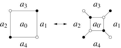
Let us designate the faces around face 0 by the numbers 1, 3, 2 and 4. Each of these faces gains two new edges. In the new graph $\Gamma^{\prime}$, there are faces $1^{\prime},2^{\prime},3^{\prime}$ and $4^{\prime}$ each with two more edges than the corresponding face $1,2,3,4$. There is a face $0^{\prime}$ which is also square. Each other face $f$ of $\Gamma$ corresponds to a face $f^{\prime}$ of $\Gamma^{\prime}$ with the same number of edges as $f$. There are four new neighboring relations among faces: $1^{\prime},2^{\prime},3^{\prime}$ and $4^{\prime}$ are neighbors in cyclic order, in addition to any neighboring relations that may have held before. The point of urban renewal is to give a corresponding adjustment of the weights that preserves $\mu_{d}$. This is most easily done in terms of the $A$ variables. The following proposition was proved in [19].

Proposition 2.1 (urban renewal).

Suppose 0 is a quadrilateral face of $\Gamma$. Let $\Gamma^{\prime}$ be constructed from $\Gamma$ as above. Define the new pre-weight function $A:F^{\prime}\to\mathbb{C}$ by $A(f^{\prime})=A(f)$ if $f\neq 0$ and

$$A(0^{\prime}):=\frac{A(1)A(2)+A(3)A(4)}{A(0)}\,.$$

Let $\mu^{\prime}$ denote the dimer measure on $\Gamma^{\prime}$ with edge weights $\nu_{A^{\prime}}$ and $\mu$ the dimer measure on $\Gamma$ with face weights $\nu_{A}$. Then $\mu$ and $\mu^{\prime}$ may be coupled so that the sample pair $(m,m^{\prime})$ agrees on every edge other than the four edges bounding face 0 in $\Gamma$ and the eight edges touching face $0^{\prime}$ in $\Gamma^{\prime}$. $\hfill\Box$

There are several equivalent versions of urban renewal, all of which are related to each other by vertex contraction and splitting. Two of these are depicted in Figure 4.

Figure 4: Other variants of urban renewal.

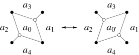
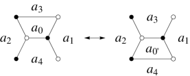
Proposition 2.2 ([9]).

The transformation of $(\Gamma,A)$ to $(\Gamma^{\prime},A^{\prime})$ under urban renewal is a mutation operation. Consequently, the final variables after any number of urban renewals are Laurent polynomials in the original variables $\{A_{f}:f\in F\}$.

For readers familiar with cluster algebras, the underlying quiver is the dual graph, with edges directed so that white vertices are on the left.

2.4 Superurban renewal transformation for the dimer model

A more complicated local transformation is the superurban renewal shown in Figure 5. Figure 6 shows how this can be decomposed into a sequence of six urban renewals.

Figure 5: Under superurban renewal the variables $a_{0},a_{1},a_{2},a_{3}$ change as indicated in (9)-(12).

Figure 6: Writing a superurban renewal as a composition of urban renewals. The stars indicate which face undergoes urban renewal

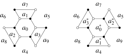
Just as urban renewal is the basis for the octahedron recurrence, we will see that superurban renewal is the basis for the hexahedron recurrence (see Section 3). In section 6 we show how superurban renewal specializes to the Y-Delta transformation for the Ising model.

Lemma 2.3.

Under a superurban renewal the $A$ variables transform as in Figure 5, with

$$a_{1}^{*} = \frac{a_{1}a_{2}a_{3}+a_{4}a_{5}a_{6}+a_{0}a_{4}a_{7}}{a_{0}a_{1}}\$$ (9)

$$a_{2}^{*} = \frac{a_{1}a_{2}a_{3}+a_{4}a_{5}a_{6}+a_{0}a_{5}a_{8}}{a_{0}a_{2}}$$ (10)

$$a_{3}^{*} = \frac{a_{1}a_{2}a_{3}+a_{4}a_{5}a_{6}+a_{0}a_{6}a_{9}}{a_{0}a_{3}}$$ (11)

$$a_{0}^{*} = \frac{a_{1}^{2}a_{2}^{2}a_{3}^{2}+a_{1}a_{2}a_{3}(2a_{4}a_{5}a_{6}+a_{0}a_{4}a_{7}+a_{0}a_{5}a_{8}+a_{0}a_{6}a_{9})+(a_{5}a_{6}+a_{0}a_{7})(a_{4}a_{5}+a_{0}a_{9})(a_{4}a_{6}+a_{0}a_{8})}{a_{0}^{2}a_{1}a_{2}a_{3}}\,.$$ (12)

Proof.

A computation using the composition of Figure 6 and the urban renewal formula from Figure 3. ∎

Iterating Proposition 2.2 proves the following result.

Corollary 2.4 (Laurent property for superurban renewal).

Under iterated superurban renewal, all new variables are Laurent polynomials in the original variables. $\hfill\Box$

3 Picturing superurban renewal via stepped surfaces

3.1 Graphs associated with stepped surfaces

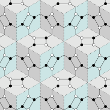
A stepped solid in $\mathbb{R}^{3}$ is a union $U$ of lattice cubes $[i,i+1]\times[j,j+1]\times[k,k+1]$ which is downwardly closed, meaning that if a cube $B$ is in $U$ then so is any translation of $B$ by negative values in any coordinate. In particular, all our stepped solids are infinite. A stepped surface is the topological boundary of a stepped solid. Every stepped surface is the union of lattice squares and every lattice square has vertex set of the form $\{v,v+e_{i},v+e_{j},v+e_{i}+e_{j}\}$ for some $v\in\mathbb{Z}^{3}$ and some integers $1\leq i<j\leq 3$. For each stepped surface $\partial U$ its $1$-skeleton $\partial U_{1}$ is a planar graph. We associate to $U$ another graph, the associated graph $\Gamma(U)$, obtained by starting with the dual graph of $\partial U_{1}$ and replacing each vertex by a small quadrilateral, as illustrated in Figure 7.

Figure 7 shows the so-called 4-6-12 graph, which is the graph $\Gamma(U)$ when $U$ is the union of all cubes lying entirely within the region $\{(x,y,z):x+y+z\leq 2\}$. For general stepped surfaces, the faces of $\Gamma(U)$ will be of two types: there is a quadrilateral face centered at the center of each face of $\partial U_{1}$ and there is a $(2k)$-gonal face centered at each vertex of $\partial U_{1}$, where $k$ is the number of faces of the surface $\partial U_{1}$ coming together at the vertex, each contributing one edge and two half-edges (“legs”). The label of the face $f$ is the coordinates of the face center or vertex at which $f$ is centered. All face labels are elements of the set

$${\mathbb{Z}^{3}_{1/2}}:=\{(x,y,z)\in(1/2)\mathbb{Z}^{3}:x+y+z\in\mathbb{Z}\}\,.$$

The canonical variables are the labels of the 4-6-12 graph, namely all elements of $\mathbb{Z}^{3}$ at levels 0, 1 or 2 and all elements of $(1/2)\mathbb{Z}^{3}$ at level 1.

Figure 7: The 4-6-12 graph is drawn on the stepped surface $U$ bounding the union of cubes up to level 2

3.2 Superurban renewal for associated graphs

Let $U$ be a stepped solid with stepped surface $\partial U$ and associated graph $\Gamma(U)$. Suppose that $(i,j,k)$ is a point of $\partial U$ which is a local minimum with respect to the height function $i+j+k$. In other words, $(i-1,j,k)$, $(i,j-1,k)$ and $(i,j,k-1)$ are all in the interior of $U$. Let $U^{+ijk}$ be the union of $U$ with the cube $[i,i+1]\times[j,j+1]\times[k,k+1]$. The following facts are easily verified by inspection.

Proposition 3.1 (superurban renewal is adding a cube).

Suppose $U$ and $(i,j,k)$ are as above.

1. The face in $\Gamma(U)$ corresponding to $(i,j,k)$ is a hexagon.

2. The graph $\Gamma(U^{+ijk})$ is obtained from the graph $\Gamma(U)$ by superurban renewal at this hexagon.

3. The variables associated with each face of $\Gamma(U)$ transform under superurban renewal according to the hexahedron recurrence (4)–(7), provided we interpret

   $$h(i,j,k) = A(i,j,k)$$

   $$h^{(x)}(i,j,k) = A(i,j+1/2,k+1/2)$$

   $$h^{(y)}(i,j,k) = A(i+1/2,j,k+1/2)$$

   $$h^{(z)}(i,j,k) = A(i+1/2,j+1/2,k)\,.$$

$\hfill\Box$

3.3 Cubic corner graph and taut dimer configurations

We now know that adding a cube to a downwardly closed stepped solid corresponds to superurban renewal on the associated graph, which corresponds to the use of the hexahedron recurrence to write the top variable in terms of lower variables. These representations commute. To state this more precisely, let $U_{0}$ be the stepped solid coincident with the closed negative orthant. The associated graph $\Gamma(U_{0})$ is called the cubic corner graph and is shown in Figure 8.

Figure 8: The cubic corner graph.

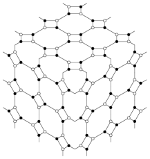
Let ${\cal L}$ be the lattice poset of all stepped solid subsets of $U_{0}$ containing all but finitely many cubes of $U_{0}$. For each $U\in{\cal L}$, one may add a finite sequence of cubes resulting in $U_{0}$. Therefore, a finite sequence of superurban renewals represents $A(0,0,0)$ in terms of the variables labeling faces and vertices of the stepped surface $\partial U$ that are in the union of the removed lattice cubes. Denote this set of variables by ${\cal I}(U)$.

Proposition 3.2.

$(i)$ The rational function $F$ representing $A(0,0,0)$ in terms of the variables in ${\cal I}$ is a Laurent polynomial. $(ii)$ If $U^{\prime}\subset U$ in ${\cal L}$ and the representation of each variable $w\in{\cal I}(U)$ in terms of variables in ${\cal I}(U^{\prime})$ is substituted into $F$, the resulting Laurent polynomial is the representation of $A(0,0,0)$ in terms of variables in ${\cal I}(U^{\prime})$.

Proof.

By Proposition 3.1, the expression $F$ is obtained by a sequence of superurban renewals. By definition, each of these is a sequence of six urban renewals, hence part $(i)$ follows from Proposition 2.2. Part $(ii)$ is a consequence of the lack of relations among the variables in any stepped surface. ∎

Our combinatorial interpretations of these formulae take place on the associated graphs $\Gamma(U)$. An example to keep in mind is $U_{-n}$, defined to be those cubes of $U_{0}$ lying entirely within the halfspace $\{(x,y,z)\,:\,x+y+z\leq-n\}$. This solid and its associated graph are illustrated for $n=-1$ (only the top cube removed) in Figure 9.

Figure 9: After removing the topmost cube.

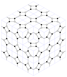
This solid is a subset of $Z_{-n}$, the stepped solid defined by $x+y+z\leq-n$, whose associated graph is isomorphic to the 4-6-12 graph of Figure 7. The labels of $Z_{-n}$ are precisely the points of $\mathbb{Z}^{3}$ at levels $-n-2,-n-1$ and $-n$ together with the half integer points at level $-n-1$. The hexahedron recurrence imposes no relations on this set of variables, hence from the point of view of determining $A(0,0,0)$ as a function of the variables in ${\cal I}(U_{-n})$, we might equally well think of the initial variables as being all of those in $\Gamma(Z_{-n})$.

We define a double-dimer configuration $m_{0}$ on the cubic corner graph $\Gamma_{0}$ as in Figure 10.

Figure 10: The initial double-dimer configuration $m_{0}$ on $\Gamma_{0}$.

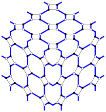
This configuration $m_{0}$ plays the role of our initial configuration. This configuration has the following property. If we erase a finite piece of $m_{0}$, there is a unique way to complete it to a double-dimer configuration which has the same boundary connections, that is, connections between far-away points. For $U\in{\cal L}$, we say that a double-dimer configuration on $\Gamma(U)$ is taut if it has the same boundary connections as $m_{0}$, that is, it is identical to $m_{0}$ far from the origin and there is a bijection between its bi-infinite paths and those of $m_{0}$ which is the identity near $\infty$. There are a finite number of taut configurations. See Figure 11 for one such on $\Gamma(U_{-1})$.

Figure 11: A taut double-dimer configuration on $\Gamma(U_{-1})$. Doubled edges are thicker.

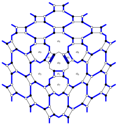
4 Main formula

Given a taut dimer configuration $m$, let $c(m)$ denote the number of loops in $m$ and define $c(m;i,j,k):=L(i,j,k)-2-d(m;i,j,k)$ where $L(i,j,k)$ is the number of edges in the face $(i,j,k)$ and $d(m;i,j,k)$ is the number of dimers lying along the face $(i,j,k)$ in the matching $m$. Define the weight of a taut configuration $m$ to be

$$2^{c(m)}\prod_{(i,j,k)\in{\cal I}(U)}A(i,j,k)^{c(m;i,j,k)}$$

where $c(m)$ is the number of nontrivial loops in $m$. In the configuration $m_{0}$, all quadrilateral faces have 2 dimers and all octagonal faces have 6 dimers, so the only face $(i,j,k)$ with $c(m_{0};i,j,k)\neq 0$ is the hexagonal face which has 3 dimers and $c(m_{0};0,0,0)=6-2-3=1$. Any taut configuration differs from $m_{0}$ in finitely many places, hence its weight has finitely many variables appearing in it. For example, the configuration of Figure 11 has weight $\displaystyle{\frac{a_{4}^{2}a_{5}a_{6}a_{7}}{a_{0}a_{1}a_{2}a_{3}}}$.

Theorem 4.1.

Fix any $U\in{\cal L}$ and let ${\cal I}(U)$ be the labels of $\Gamma(U)$. Use the notation $m\preceq U$ to signify that $m$ is a taut double-dimer configuration on $\Gamma(U)$. Then the representation of $A(0,0,0)$ as a Laurent polynomial in the variables in ${\cal I}(U)$ is given by

$$A(0,0,0)=\sum_{m\,\preceq\;U}2^{c(m)}\prod_{(i,j,k)\in{\cal I}(U)}A(i,j,k)^{c(m;i,j,k)}\,.$$ (13)

Specializing to $U_{-n}$ and $A(i,j,k)=1$ for all $i,j,k$ with $-n-2\leq i+j+k\leq-n$ gives the formula

$$A(0,0,0)=\sum_{m\,\preceq\;U_{-n}}2^{c(m)}\,.$$

Remark.

These formulae are translation-invariant, once one accounts for the distinguished role played by $(0,0,0)$ in $\Gamma_{0}$. Let $(r,s,t)$ be any point of $\mathbb{Z}^{3}$ and $U$ be any lattice solid obtained by removing finitely many cubes from the top of the orthant $\{x\leq r,y\leq s,z\leq t\}$. Then $A(r,s,t)$ is a Laurent polynomial in the set ${\cal I}(U)$ of labels in $\Gamma(U)$ and (13) holds for $A(r,s,t)$ in place of $(0,0,0)$.

Proof.

We induct on $U$. It is true for $U=U_{0}$: there is one configuration, $m_{0}$, with $c(m_{0};i,j,k)=1$ if $i=j=k=0$ and zero otherwise. The sum is therefore equal to $A(0,0,0)$, yielding the identity $A(0,0,0)=A(0,0,0)$ which is the correct representation.

For the induction to run, we need to see that the conclusion remains true if we remove a maximal cube. This corresponds to a superurban renewal, which is a composition of ordinary urban renewals with additional vertex splittings and contractions, depending on which version of ordinary urban renewal is used. Under a vertex splitting, two faces increase in length by $2$ and get two additional dimers on them. Thus their contribution does not change. A similar argument holds for vertex contraction.

Consider an urban renewal of type shown in Figure 3. There are several cases to consider, see Figure 12, depending on the various possible boundary connections. In the first case, the ratio of monomials on the right side and left side of the equation is

$$\frac{a_{5}^{2}a_{1}^{2-4}a_{2}^{2-4}a_{3}^{2-4}a_{4}^{2-4}}{2a_{0}^{-2}a_{1}^{-1}a_{2}^{-1}a_{3}^{-1}a_{4}^{-1}+a_{0}^{-2}a_{1}^{-2}a_{2}^{-2}a_{3}^{0}a_{4}^{0}+a_{0}^{-2}a_{1}^{0}a_{2}^{0}a_{3}^{-2}a_{4}^{-2}}=\frac{a_{5}^{2}a_{0}^{2}}{a_{1}a_{2}a_{3}a_{4}(2+\frac{a_{3}a_{4}}{a_{1}a_{2}}+\frac{a_{1}a_{2}}{a_{3}a_{4}})}=1\,.$$

In the second case, the ratio is

$$\frac{a_{5}^{1}a_{1}^{2-4}a_{2}^{2-3}a_{3}^{2-3}a_{4}^{2-3}}{a_{0}^{-1}(a_{1}^{-1}a_{2}^{0}a_{3}^{-1}a_{4}^{-1}+a_{1}^{-2}a_{2}^{-1}a_{3}^{0}a_{4}^{0})}=\frac{a_{0}a_{5}}{a_{1}a_{2}+a_{3}a_{4}}=1\,.$$

The remaining five cases are similar. These cover all possible cases (up to rotations).

Figure 12: Checking consistency of urban renewal formulas and $A$ monomials.

∎

5 Limit shapes

In this section we specialize values of the initial variables in several natural ways and study the behavior of the resulting ensembles. Let $\ell:\mathbb{Z}^{d}\to\mathbb{Z}$ be a linear function which we regard as time. A function $f:\mathbb{Z}^{d}\to\mathbb{Z}$ is said to be (spatially) isotropic if $f(v)$ depends only on $\ell(v)$. Solutions to recurrences that are isotropic and have the particularly simple form $f(v)=\gamma^{\ell(v)^{k}}$ lead to linear recurrences for the formal logarithmic derivatives $(\partial/\partial t)\log f(v,t)$; these have probabilistic interpretations and satisfy limit shape theorems. We begin by identifying the exponent $\delta$ for which such a solution exists.

5.1 Isotropic solutions and homogeneity

In order to discuss general $\mathbb{Z}^{d}$-invariant algebraic recurrences some notation is required. Let ${\cal A}$ be a finite index set, let $\{E_{\alpha}:\alpha\in\mathbb{Z}\}$ be a finite collection of multisets of elements of $\mathbb{Z}^{d}$, and let $\{c_{\alpha}:\alpha\in{\cal A}\}$ be constants. Denote the multiset union by $E:=\bigcup_{\alpha\in{\cal A}}E_{\alpha}$. For each $v\in\mathbb{Z}^{d}$, define a polynomial $P_{(v)}$ on indeterminates $\{x_{w}:w\in\mathbb{Z}^{d}\}$ by the equation

$$P_{(v)}=\sum_{\alpha\in{\cal A}}c_{\alpha}\prod_{w\in E_{\alpha}}x_{v+w}\,.$$ (14)

A lattice function $f:\mathbb{Z}^{d}\to\mathbb{C}$ is said to satisfy the algebraic recurrence $P=\{P_{(v)}:v\in\mathbb{Z}^{d}\}$ if at all $v\in\mathbb{Z}^{d}$, $P_{(v)}$ vanishes upon setting $x_{w}=f(w)$ for all $w\in\mathbb{Z}^{d}$. Say that the recurrence is $k$-homogeneous with respect to the linear functional $\ell:\mathbb{Z}^{d}\to\mathbb{Z}$ if there are constants $\beta_{0},\ldots,\beta_{k}$ such that for each $\alpha\in{\cal A}$ and each $0\leq j\leq k$,

$$\sum_{w\in E_{\alpha}}\ell(w)^{j}=\beta_{j}\,.$$

For instance, the recurrence is 0-homogeneous if $|E_{\alpha}|=\beta_{0}$, that is, if the polynomials $P_{(v)}$ are homogeneous of degree $\beta_{0}$. The degree of homogeneity of the recurrence $P$ is the maximum $\delta$ such that $P$ is $\delta$-homogeneous.

Example 5.1.

The octahedron recurrence (1) is 1-homogeneous with respect to the height function $\ell(i,j,k)=j+k$. To see this, put the recurrence in the form of (14) by taking $E_{1}=\{(1,0,0),(0,1,1)\}$, $E_{2}=\{(0,1,0),(1,0,1)\}$ and $E_{3}=\{(0,0,1),(1,1,0)\}$. The corresponding multisets of heights are $\{0,2\},\{1,1\}$ and $\{1,1\}$. The sums of the zero powers of the heights are the constant $\beta_{0}=2$. The sums of the first powers of the heights are the constant $\beta_{1}=2$. The sums of the squares of the heights are not constant (4, 2 and 2) therefore the degree of homogeneity of the octahedron recurrence with respect to $\ell(i,j,k)=j+k$ is 1.

The degree of homogeneity of a recurrence tells us for which power $\delta$ we can expect a solution to the recurrence of the form $f(v)=\gamma^{\ell(v)^{\delta}}$. These solutions are the ones for which we can most easily compute corresponding linear recurrences for the the derivatives $(\partial/\partial t)f(v,t)$.

Proposition 5.2.

Suppose the degree of homogeneity of the recurrence $P$ is $\delta-1$. Suppose further that $\sum_{\alpha\in S}c_{\alpha}$ is nonvanishing for at least two equivalence classes $S=S_{m}=\{\alpha:\sum_{w\in E_{\alpha}}\ell(w)^{\delta}=m\}$. Then there is a number $\gamma\neq 0$ such that $f(v)=\gamma^{\ell(v)^{\delta}}$ satisfies $P$ at every $v\in\mathbb{Z}^{d}$. In fact $f(v)=\gamma^{q(\ell(v))}$ satisfies $P$ for every monic polynomial $q$ of degree $\delta$.

Proof.

Let $q$ be a monic polynomial of degree $\delta$ and define $f(v)=f_{q}(v)=\gamma^{q(\ell(v))}$. This satisfies $P$ at $v$ if and only if

$$\sum_{\alpha\in{\cal A}}c_{\alpha}\gamma^{\sum_{w\in E_{\alpha}}q(\ell(v+w))}=0\,.$$ (15)

For $j<\delta$,

$$\sum_{w\in E_{\alpha}}\ell(v+w)^{j} = \sum_{w\in E_{\alpha}}(\ell(v)+\ell(w))^{j}$$

$$= \sum_{w\in E_{\alpha}}\sum_{i\leq j}\binom{j}{i}\ell(v)^{i}\ell(w)^{j-i}$$

$$= \sum_{w\in E_{\alpha}}\sum_{i\leq j}\binom{j}{i}\beta_{j-i}\ell(v)^{i}$$

$$:= C(v)$$

and factoring out $\gamma^{C(v)}$ from (15) leaves

$$\sum_{\alpha\in{\cal A}}c_{\alpha}\gamma^{\sum_{w\in E_{\alpha}}(\ell(v+w))^{\delta}}=0\,.$$ (16)

Again we may decompose the power $\ell(v+w)^{\delta}=(\ell(v)+\ell(w))^{\delta}$, this time arriving at

$$\sum_{w\in E_{\alpha}}\ell(v+w)^{\delta}=\sum_{w\in E_{\alpha}}\ell(w)^{\delta}+\sum_{1\leq i\leq\delta}\binom{\delta}{i}\beta_{\delta-i}\ell(v)^{i}:=\ell(w)^{\delta}+D(v)\,.$$

Factoring out $\gamma^{D(v)}$ from (16) leaves

$$\sum_{\alpha\in{\cal A}}c_{\alpha}\gamma^{\sum_{w\in E_{\alpha}}(\ell(w))^{\delta}}=0\,.$$ (17)

This no longer depends on $v$, and is not a monomial because we have assumed that $P$ is not $\delta$-homogeneous. Therefore, there is at least one nonzero value of $\gamma$ for which (17) holds, and this finishes the proof. ∎

5.2 Recurrence for the derivative

Suppose that each set $E_{\alpha}$ resides in the $\ell$-nonnegative halfspace $\mathbb{Z}^{d}_{\ell}:=\{v\in\mathbb{Z}^{d}:\ell(v)\geq 0\}$, and suppose further that the values $\{f(v):v\in\mathbb{Z}^{d}_{\ell}\}$ all depend smoothly on some parameter $t$. Consider the logarithmic derivative $g(v)=(d/dt)\log f(v)=f^{\prime}(v)/f(v)$, which is defined whenever $f(v)\neq 0$. We claim that $g$ satisfies a linear recurrence with constant coefficients.

Proposition 5.3.

Suppose that $P$ is $(\delta-1)$-homogeneous but not $\delta$-homogeneous and choose $\gamma$ according to Proposition 5.2 so that $f_{0}(v)=\gamma^{\ell(v)^{\delta}}$ solves $P$. Let $f(t,v)$ be smooth in $t$ with $f(0,v)=f_{0}(v)$ and let $g(v)=(d/dt)\log f(t,v)|_{t=0}$. Then

$$\sum_{\alpha\in{\cal A}}c_{\alpha}^{\prime}\sum_{w\in E_{\alpha}}\;g(v+w)=0$$ (18)

for all $v\in\mathbb{Z}^{d}_{\ell}$, where

$$c_{\alpha}^{\prime}=c_{\alpha}\gamma^{\ell(\alpha)}$$

and

$$\ell(\alpha):=\sum_{w\in E_{\alpha}}\ell(w)^{\delta}\,.$$

Proof.

Differentiating the recurrence at $v$ gives

$$0 = \left(\frac{d}{dt}\right)_{t=0}\sum_{\alpha\in{\cal A}}c_{\alpha}\prod_{w\in E_{\alpha}}x_{v+w}$$

$$= \sum_{\alpha\in{\cal A}}c_{\alpha}\left(\sum_{w\in E_{\alpha}}g(v+w)\right)\prod_{w\in E_{\alpha}}f(v+w)$$

$$= \sum_{\alpha\in{\cal A}}c_{\alpha}\sum_{w\in E_{\alpha}}g(v+w)\gamma^{\sum_{w\in E_{\alpha}}\ell(v+w)^{\delta}}\,.$$

The sum $\sum_{w\in E_{\alpha}}\ell(v+w)^{\delta}$ is equal to $D(v)+\ell(\alpha)$, whence, factoring out $\gamma^{D(v)}$ from the last equation proves the proposition. ∎

The characteristic polynomial of a recurrence $\sum_{w\in E}b_{w}g(v+w)=0$ is the Laurent polynomial $\sum_{w\in E}b_{w}x^{w}$, where $x^{w}$ denotes the monomial $x_{1}^{w_{1}}\cdots x_{d}^{w_{d}}$. In particular, the characteristic polynomial of (18) is

$$H=H_{P}=\sum_{\alpha\in{\cal A}}c_{\alpha}^{\prime}\sum_{w\in E_{\alpha}}x^{w}\,.$$

Example 5.4.

For the octahedron recurrence, let $E_{1}:=\{(1,0,0),(0,1,1)\}$, $E_{2}:=\{(0,1,0),(1,0,1)\}$ and $E_{3}:=\{(0,0,1),(1,1,0)\}$ and denote these six vectors by $w_{1},\ldots,w_{6}$ respectively. Then $\ell(1)=4,\ell(2)=2,\ell(3)=2$. The equation for $\gamma$ is $\sum_{\alpha}c_{\alpha}^{\prime}|E_{\alpha}|=0$, which is $2\gamma^{4}-4\gamma^{2}=0$, so $\gamma=\sqrt{2}$. The linear recurrence on derivatives is then given by

$$2[g(v+w_{1})+g(v+w_{2})]-g(v+w_{3})-g(v+w_{4})-g(v+w_{5})-g(v+w_{6})=0\,.$$

Dividing by 2, we see that the sum of the $x$ and $yz$ points is equal to one half the sum of the other four points in any elementary octahedron. This recurrence has characteristic polynomial $2(x+yz)-(y+z+xz+xy)$.

Example 5.5 (cube recurrence).

Let $w_{1},\ldots,w_{8}$ denote

$$(0,0,0),(1,1,1),(1,0,0),(0,1,1),(0,1,0),(1,0,1),(0,0,1),(1,1,0)$$

respectively and let $E_{j}=\{w_{2j-1},w_{2j}\}$ for $j=1,2,3,4$. This puts the cube recurrence (2) in standard form with $c_{1}=1$ and $c_{2}=c_{3}=c_{4}=-1$. With $\ell(i,j,k)=i+j+k$, the cube recurrence has degree of homogeneity equal to $1$. The values of $\ell(\alpha)=\sum_{w\in E_{\alpha}}\ell(w)^{2}$ for $\alpha=1,2,3,4$ are $9,5,5,5$ and the resulting equation for $\gamma$ is $\gamma^{9}-3\gamma^{5}$ which has one positive solution $\gamma=3^{1/4}$. This leads to values for $c_{\alpha}^{\prime}$ (we may divide everything by $3^{5/4}$) of $3,1,1$ and $1$ respectively. Thus the recurrence for the derivatives is given by

$$g(v)+g(v+w_{2})=\frac{1}{3}\left(\sum_{j=3}^{8}g(v+w_{j})\right)$$

and the characteristic polynomial for the cube recurrence with respect to $\ell=i+j+k$ is

$$3(xyz+1)-(x+y+z+xy+xz+yz)\,.$$

5.3 Behavior of linear recurrences

5.3.1 Boundary conditions

With the right boundary conditions, the linear recurrence (18) will have tractable asymptotics and a limiting shape. This is assured when the boundary conditions are such that (18) holds for all but finitely many $v\in\mathbb{Z}^{d}$. The most common way this arises is as follows. Re-indexing if necessary, suppose that $0\in E$ (recall $E=\bigcup_{\alpha}E_{\alpha}$), suppose that $\ell$ attains its unique maximum there, and let $-m$ denote the minimum value of $\ell$ on $E$. The recurrence (18) determines $g(v)$ as a linear function of $\{g(v+w):0\neq w\in E\}$. A canonical boundary condition is to take $g(w)=0$ when $\ell(w)<0$, to take $g(0)=1$ and to define $g$ everywhere else by the recurrence. In this case (18) holds everywhere except at the origin.

Define a $d$-variable generating function

$$F(x):=\sum_{v}g(v)x^{v}$$

where $x^{v}$ denotes the monomial $x_{1}^{v_{1}}\cdots x_{d}^{v_{d}}$. Let $H$ denote the characteristic polynomial of the recurrence. The fact that (18) holds except at finitely many points implies that the generating function $F$ satisfies $HF=G$ where $G$ is a Laurent polynomial.

Example 5.6 (octahedron recurrence, continued).

If we impose the octahedron recurrence everywhere except at the origin, setting the right-hand side of (18) equal to 1 at the origin and setting $g(v)=0$ when $\ell(v)\leq 2$ except for $\ell(0,1,1)=1$, then $HF=x_{2}x_{3}$, whence

$$F=\frac{yz}{H}=\frac{yz}{2x+2yz-y-z-xz-xy}\,.$$

The usual form of the octahedron recurrence differs from ours by an affine transformation, whence one usually sees (e.g. for the Aztec Diamond creation rate generating function)

$$F(x,y,z)=\frac{z}{2-(x+x^{-1}+y+y^{-1})z+2z^{2}}\,;$$

see [6] or [1, Section 4.1] for the generating function in this form.

5.3.2 Coefficient asymptotics

Laurent series for rational functions obey limit laws. A brief summary of the necessary background is as follows; see, e.g., [17, Chapter 7]. Let $H$ be a Laurent polynomial vanishing at $(1,\ldots,1)$. The amoeba of $H$ is the image in $\mathbb{R}^{d}$ of the complex zero set of $H$ under the log-modulus map $(z_{1},\ldots,z_{d})\to(\log|z_{1}|,\ldots,\log|z_{d}|)$. The components of the complement of the amoeba are convex. Assume that there is one component, $B$, with the origin on the boundary. Any rational function $G/H$ has a Laurent series $\sum_{v}a_{v}x^{v}$ convergent in the domain $\{\exp(x+iy):x\in B\}$.

The following further assumptions on $H$ put the asymptotic behavior in the class of so-called cone points, discussed in [1] and [17, Chapter 11]. Let $K$ be the convex cone of vectors for which all sufficiently small positive multiples are in $B$. The cone $K$ is a cone of hyperbolicity for $H$. Let $K^{*}$ denote the dual cone $\{w\in\mathbb{R}^{d}:\langle w,v\rangle\leq 0~{}\forall v\in K\}$. We assume that $H$ is irreducible in the local ring at $(1,\ldots,1)$ and that $K^{*}$ has nonempty interior.

Theorem 5.7.

Let $F,G,H,B,K$ and $K^{*}$ be as above. Assume that the zero set of $H$ touches the closed unit polydisk only at $(1,\dots,1)$. Then

1. The coefficients $a_{v}$ decay exponentially in $|v|$ when $v\notin K^{*}$, the exponential rate being uniform if $v/|v|$ is contained in a compact set disjoint from $K^{*}$.

2. If $G(1,\ldots,1)=1$ then on $K^{*}$, $a_{v}\sim\Psi(v)$ (the ratio tends to $1$) where $\Psi$ is the inverse Fourier transform of $1/\overline{H}$, the leading homogeneous part of $H$ at $(1,\ldots,1)$.

3. The inverse Fourier transform $\Psi$ is homogeneous of degree $\deg(\overline{H})-d$ .

4. If $G$ vanishes to degree $\delta$ at $(1,\ldots,1)$ then on $K^{*}$, $a_{v}\sim\Psi_{G}$, where $\Psi_{G}$ is a linear combination of partial derivatives of order $\delta$ of $\Psi$.

If instead the zero set of $H$ intersects the unit torus in finitely many points then $K^{*}$ is the union of the dual cones at each zero of $H$, the coefficients decay exponentially away from $K^{*}$, and the leading asymptotic on $K^{*}$ is obtained by summing $\Psi$ over the finitely many contact points of the zero set with the unit torus.

Sketch of proof:.

The first part is essentially the Paley-Wiener Theorem. It was proved in the special case of cube groves (the cube recurrence) in [18]. The general proof may be found in [17, Chapter 8]. The second part is proved as [1, Lemma 6.3]. There, hypotheses are assumed to restrict the vanishing degree of $H$ at $(1,\ldots,1)$ to 2, but in fact the proof is valid for any degree. The third part follows from the general theory of inverse Fourier transforms, and the fourth part is [1, Proposition 6.2], again removing the restriction on the degree of vanishing of $H$ at $(1,\ldots,1)$. ∎

It is not possible to conclude that the support of $\Psi$ is all of the cone $K^{*}$. More detailed information is given by computing the critical sets. The definition of the dual cones and critical sets are somewhat complicated, relying on hyperbolicity theory. We will not duplicate them here but will quote the result. Again, the proof may be taken from [1], noting that the unit torus is a minimal torus, and that the finiteness assumption on $W(v)$ satisfies the hypotheses of Theorem 5.8 there.

Definition 5.8 (critical set).

For each $v$ in the interior of $K^{*}$, let $W(v)$ denote the set of $z$ in the unit torus such that $v$ is in the dual cone to $H$ at $z$ as defined in [1, Definition 2.21]. In particular when $\nabla H(z)\neq 0$, the point $z$ is in $W(v)$ exactly when $v$ is a scalar multiple of the logarithmic gradient $(z_{1}\partial H/\partial z_{1},\ldots,z_{d}\partial H/\partial z_{d})(z)$. Let $K^{\dagger}\subseteq K^{*}$ denote the subset of $v$ such that $W(v)$ is nonempty.

Corollary 5.9.

Let $F,G,H,B,K,K^{*}$ and $K^{\dagger}$ be as discussed above. Replace the hypothesis of Theorem 5.7 that $H$ vanishes finitely often on the closed polydisk by the following hypotheses:

1. The zero set of $H$ is disjoint from the open unit polydisk;

2. For each $v\in K^{*}$, the set $W(v)$ is finite.

Whenever $H(z)=0$, let $\overline{H}_{z}$ denote the homogeneous part of $H$ at $z$ and let $\Psi_{z}$ denote the inverse Fourier transform of $\overline{H}_{z}$. Then for $v\in K^{\dagger}$, $a_{v}$ is given asymptotically by the $\sum_{z\in W(v)}\Psi_{z}$. The coefficients $a_{v}$ tend to zero exponentially rapidly when $v$ goes to infinity and remains in any closed subcone disjoint from the closure of $K^{\dagger}$. $\hfill\Box$

The phase boundary for a statistical mechanical system with generating function $F$ is the boundary between exponential and non-exponential decay of probabilities, which in most cases is $\partial K^{\dagger}$. When $K^{\dagger}=K^{*}$, the phase boundary is equal to $\partial K^{*}$ and is not hard to compute: it is a component of the real algebraic hypersurface dual to the zero set of $\overline{H}$ in projective $(d-1)$-space. When $d=3$, the boundary of $K^{*}$ is an algebraic curve in $\mathbb{RP}^{2}$. This curve may be computed from $H(x,y,z)$ be setting $z=-ax-by$ and eliminating $x$ and $y$ from the simultaneous polynomial equations

$$H=0\;\;;\;\;\frac{\partial H}{\partial x}=0\;\;;\;\;\frac{\partial H}{\partial y}=0\;.$$ (19)

5.4 Application to the hexahedron recurrence

We now apply the results of the last three subsections to the hexahedron recurrence. We have developed these results independently of the specific recurrence for several reasons. First, the methods are more general and it is good to see them in the abstract. Secondly, the hexahedron recurrence is not $\mathbb{Z}^{d}$-invariant but invariant under a sublattice of finite index. Because of this, it is not easy to see what is going on if one begins with the hexahedron recurrence. The exposition is clearest for general $\mathbb{Z}^{d}$-invariant recurrences, after which we may work the hexahedron recurrence along similar lines. We do not develop a general theory of periodic recurrences for finite index sublattices because the notation is even messier. We first compute the isotropic solutions, then compute the linear recurrences for the derivative, then prove limit shape results.

5.4.1 Isotropic solution

Let $\ell(i,j,k)=i+j+k$. An isotropic set of initial varibles ${\cal I}$ is given by the 4-6-12 graph: those $(i,j,k)$ with $0\leq i+j+k\leq 2$. The hexahedron recurrence, beginning with these variables, preserves the isotropy. Therefore, the solution will be described by constants $A_{n},B_{n}:n\geq 0$ such that $f(i,j,k)=A_{n}$ for integer points with $i+j+k=n$ and $f(i,j,k)=B_{n}$ for half-integer points with $i+j+k=n+1$. We will solve this general recursion, then specialize to solutions of the form $A_{n}=\gamma^{n},B_{n}=\kappa\gamma^{n}$. The initial conditions $A_{0},A_{1},A_{2}$ and $B_{0}$ and the hexahedron recurrence determine $A_{n}$ and $B_{n}$ for all positive $n$. The recurrence becomes

$$A_{n} = \frac{2A_{n-2}^{3}B_{n-3}^{3}+3A_{n-3}A_{n-1}A_{n-2}B_{n-3}^{3}+A_{n-2}^{6}+3A_{n-3}A_{n-1}A_{n-2}^{4}+3A_{n-3}^{2}A_{n-1}^{2}A_{n-2}^{2}+A_{n-3}^{3}A_{n-1}^{3}+B_{n-3}^{6}}{A_{n-3}^{2}B_{n-3}^{3}}$$

$$B_{n} = \frac{A_{n}^{3}+A_{n-1}A_{n}A_{n+1}+B_{n-1}^{3}}{A_{n-1}B_{n-1}}.$$

The values of $A_{3},B_{1}$ and $B_{2}$, are determined by the initial conditions, but we may still use them in formulae for the remaining $A$ and $B$ values, leading to a mysteriously simple solution to the recurrence.

$$A_{4}=\frac{A_{0}A_{3}^{2}}{A_{1}^{2}},A_{5}=\frac{A_{0}^{2}A_{3}^{4}}{A_{1}^{3}A_{2}^{2}},A_{6}=\frac{A_{0}^{4}A_{3}^{6}}{A_{1}^{6}A_{2}^{3}},\dots$$

$$B_{3}=\frac{A_{0}B_{1}B_{2}^{2}}{A_{2}B_{0}^{2}},B_{4}=\frac{A_{0}^{2}B_{2}^{4}}{A_{2}^{2}B_{0}^{3}},B_{6}=\frac{A_{0}^{4}B_{1}B_{2}^{6}}{A_{2}^{4}B_{0}^{6}},\dots$$

and generally one can verify by induction that

$$A_{n}=\frac{A_{0}^{\lfloor(n-2)^{2}/4\rfloor}A_{3}^{\lfloor(n-1)^{2}/4\rfloor}}{A_{1}^{\lfloor((n-1)^{2}-1)/4\rfloor}A_{2}^{\lfloor((n-2)^{2}-1)/4\rfloor}}.$$

$$B_{n}=\frac{A_{0}^{\lfloor(n-1)^{2}/4\rfloor}B_{1}^{\frac{1}{2}(1-(-1)^{n})}B_{2}^{\lfloor n^{2}/4\rfloor}}{A_{2}^{\lfloor(n-1)^{2}/4\rfloor}B_{0}^{\lfloor(n^{2}-1)/4\rfloor}}\,.$$

This can be written as

$$A_{2n} = \frac{A_{0}^{(n-1)^{2}}A_{3}^{n^{2}-n}}{A_{1}^{n^{2}-n}A_{2}^{n^{2}-2n}}$$ (20)

$$A_{2n+1} = \frac{A_{0}^{n^{2}-n}A_{3}^{n^{2}}}{A_{1}^{n^{2}-1}A_{2}^{n^{2}-n}}$$ (21)

$$B_{2n} = \frac{A_{0}^{n^{2}-n}B_{2}^{n^{2}}}{A_{2}^{n^{2}-n}B_{0}^{n^{2}-1}}$$ (22)

$$B_{2n+1} = \frac{A_{0}^{n^{2}}B_{1}B_{2}^{n^{2}+n}}{A_{2}^{n^{2}}B_{0}^{n^{2}+n}}\,.$$ (23)

The simplest nontrivial solution to this recursion and the one in the form of which we spoke earlier is

$$A_{n}=3^{n^{2}/2},B_{n}=2\cdot 3^{(n+1)^{2}/2}\,.$$ (24)

There is another reasonably simple solution with a more direct combinatorial meaning. This is obtained by setting the initial variables $A_{0},A_{1},A_{2},B_{0}$ all equal to 1. This implies $A_{3}=14,B_{1}=3$ and $B_{2}=14$ and produces the result

$$A_{2n} = 14^{n(n-1)}$$ (25)

$$A_{2n+1} = 14^{n^{2}}$$

$$B_{2n} = 14^{n^{2}}$$

$$B_{2n+1} = 3\times 14^{n(n+1)}\,.$$

Setting the initial $A$ variables equal to 1 amounts to setting all the edge weights $\nu(e)$ equal to 1 in $\Gamma(U)$, as dictated by change of variables (8). By Theorem 4.1, $A(0,0,0)$ counts taut double-dimer configurations of $\Gamma(U_{-n})$, with the weight of $m$ counted as $2^{c(m)}$ when the canonical initial variables are set to 1. By translation invariance, if $i+j+k=n+2$ and variables at levels 0, 1 and 2 are set to 1, then $A(i,j,k)$ counts taut double-dimer configurations in a graph isomorphic to $\Gamma(U_{-n})$, again with weights $2^{c(m)}$. Evaluating $A(i,j,k)=A_{n+2}=14^{(n/2)(n/2+1)}$ if $n$ is even and $14^{(n/2)(n/2+1)+1/4}$ if $n$ is odd. Thus we have proved:

Corollary 5.10.

The number of taut double-dimer configurations of $\Gamma(U_{-n})$, weighted by $2^{c(m)}$, is equal to

$$14^{\frac{n}{2}\left(\frac{n}{2}+1\right)+\frac{1}{4}\delta_{{\rm odd}}(n)}\,.$$

5.4.2 Recurrence for the derivative

Let us interpret Proposition 5.3 in the context of statistical mechanical ensembles. Suppose that over the set $E=\bigcup_{\alpha}E_{\alpha}$, the function $\ell$ has a minimum value of 0 and a maximum value of $J$. Suppose further that $P$ is an algebraic recurrence that determines the values of $\{f(v):\ell(v)\geq J\}$ in terms of initial values $\{f(v):0\leq\ell(v)<J\}$. Consider $t=f(0,\ldots,0)$ to be variable while all other initial conditions remain fixed at $f(v)=\gamma^{\ell(v)^{k}}$. Applying Proposition 5.3 gives the constant coefficient linear recurrence (18) for the logarithmic derivatives of $f(v)$. Specializing further to the case $f(v)=A(v)$ for one of the Laurent recurrences we have studied, the monomials in the expression of $A(v)$ in terms of initial variables correspond to configurations, the value $A(v)$ is the partition function for all configurations. The logarithmic derivative $\displaystyle{\frac{1}{A(v)}\;\frac{\partial A(v)}{\partial A(0,0,0)}}$ at the initial conditions $f(v)=\gamma^{\ell(v)^{k}}$ may be interpreted as the expected value of the exponent on the term $A(0,0,0)$ in the statistical mechanical ensemble in which the probability of the configuration $\xi$ is $M_{\xi}(v)/A(v)$ where $M_{\xi}$ is the monomial corresponding to $\xi$.

We now apply this to the hexahedron recurrence and the double-dimer ensemble. We choose initial conditions (24) rather than (25) because these correspond to the solution $f(v)=\gamma^{\ell(v)}$ of Proposition 5.2 with $\gamma(i,j,k)=i+j+k$. The logarithmic derivative $g(i,j,k)=A(i,j,k)^{-1}\partial A(i,j,k)/\partial A(0,0,0)$ is the expected number of dimers lying along the face at the origin in a double-dimer configuration picked from all taut configurations on $\Gamma_{ijk}$ according to the double-dimer measure $\mu_{dd}$ corresponding to the initial conditions (24). By translation invariance, this is the same as the expected number of dimers lying along the face centered at $(-i,-j,-k)$ on the graph $\Gamma(U_{-i-j-k})$. We may then ask about the limiting shape function, that is, about the values of $g(i,j,k)$ as $n=i+j+k\to\infty$ with $(i/n,j/n,k/n)\to(\alpha_{1},\alpha_{2},\alpha_{3})$ in the 2-simplex.

Taking the logarithmic derivative of the four recurrence relations and plugging in the initial conditions (24) gives the linear system

$$g_{(123)} = -g+\frac{1}{3}(g_{(1)}+g_{(2)}+g_{(3)}+g_{(23)}+g_{(13)}+g_{(12)})$$

$$g^{(x)}_{(1)} = \frac{1}{12}\left(-9g+4g_{(1)}+g_{(2)}+g_{(3)}+3g_{(23)}-4g^{(x)}+8g^{(y)}+8g^{(z)}\right)$$

$$g^{(y)}_{(2)} = \frac{1}{12}\left(-9g+g_{(1)}+4g_{(2)}+g_{(3)}+3g_{(23)}+8g^{(x)}-4g^{(y)}+8g^{(z)}\right)$$

$$g^{(z)}_{(3)} = \frac{1}{12}\left(-9g+g_{(1)}+g_{(2)}+4g_{(3)}+3g_{(12)}+8g^{(x)}+8g^{(y)}-4g^{(z)}\right).$$

As it happens, the first equation gives a self-contained recurrence for the logarithmic derivatives at the integer points. Not only that, but the recurrence is recognizable as that arising in the cube recurrence (2). In other words, letting $F(x,y,z)=\sum g_{i,j,k}x^{i}y^{j}z^{k}$, we see that the solution to the first recurrence above with boundary conditions $g(0,0,0)=1$, $g(i,j,k)=0$ for other points $(i,j,k)$ with $i+j+k\leq 0$ and satisfying the recurrence everywhere except at $(-1-1-1)$, is

$$F(x,y,z)=\frac{G(x,y,z)}{H(x,y,z)}=\frac{1}{1+xyz-\frac{1}{3}(x+y+z+xy+xz+yz)}\,.$$

5.4.3 Limit shape

This is the same as that satisfied by the cube grove placement probabilities [18]. The boundary of the dual cone is known as the “arctic circle”, which is the inscribed circle in the triangular region $\{x+y+z=n,x,y,z\geq 0\}$. Outside of this, the placement probabilities decay exponentially while inside the arctic circle they do not. Inside, the limit function is homogeneous of degree $-1$ and is asymptotically equal to the inverse of the distance to the arctic circle in the plane normal to the $(1,1,1)$ direction [1]. We can conclude from this that with high probability, a random configuration from $\Gamma_{n}$ is equal to $m_{0}$ outside a neighborhood of size $o(n)$ of the arctic circle and that there is positive local entropy everywhere inside the arctic circle.

5.5 General double-dimer shape theorems

Different periodic initial conditions lead to different limiting shapes. In the general case we differentiate (4)-(7) and use (20)-(23) to get 8 linear equations, four for $i+j+k$ odd and four for $i+j+k$ even. When $i+j+k$ is odd let $g_{i,j,k}=e_{i,j,k}a_{i+j+k}^{-1}$ and when $i+j+k$ is even let $h_{i,j,k}=e_{i,j,k}a_{i+j+k}^{-1}$. Similarly define $g^{(x)},h^{(x)}$, and so forth. This allows us to compute the general solution assuming isotropy but not the simple form of two geometric sequences $A_{n},B_{n}$ as before.

A generic example

The sequence $\{A_{n},B_{n}\}$ is determined by $a_{0},a_{1},a_{2}$ and $b_{0}$. Let us start with a specific example (for the general case see below). Let $a_{0}=1,b_{0}=1,a_{1}=2,a_{2}=3$. Then $b_{1}=15,b_{2}=189,a_{3}=378$. The linear system is

$$g_{(123)} = \frac{1}{105}\left(84h+4(g_{(1)}+g_{(2)}+g_{(3)})+98(h_{(12)}+h_{(13)}+h_{(23)})-95(h^{(x)}+h^{(y)}+h^{(z)})\right)$$

$$h_{(123)} = \frac{1}{42}\left(-33g+46(h_{(1)}+h_{(2)}+h_{(3)})+17(g_{(12)}+g_{(13)}+g_{(23)})-38(g^{(x)}+g^{(y)}+g^{(z)})\right)$$

$$g^{(x)}_{(1)} = \frac{1}{210}\left(-126h+85g_{(1)}+g_{(2)}+g_{(3)}+84h_{(23)}-85h^{(x)}+125h^{(y)}+125h^{(z)}\right)$$

$$g^{(y)}_{(2)} = \frac{1}{210}\left(-126h+g_{(1)}+85g_{(2)}+g_{(3)}+84h_{(13)}+125h^{(x)}-85h^{(y)}+125h^{(z)}\right)$$

$$g^{(z)}_{(3)} = \frac{1}{210}\left(-126h+g_{(1)}+g_{(2)}+85g_{(3)}+84h_{(12)}+125h^{(x)}+125h^{(y)}-85h^{(z)}\right)$$

$$h^{(x)}_{(1)} = \frac{1}{15}\left(-9g+6g_{(23)}+14h_{(1)}+8h_{(2)}+8h_{(3)}-14g^{(x)}+g^{(y)}+g^{(z)}\right)$$

$$h^{(y)}_{(2)} = \frac{1}{15}\left(-9g+6g_{(13)}+8h_{(1)}+14h_{(2)}+8h_{(3)}+g^{(x)}-14g^{(y)}+g^{(z)}\right)$$

$$h^{(z)}_{(3)} = \frac{1}{15}\left(-9g+6g_{(12)}+8h_{(1)}+8h_{(2)}+14h_{(3)}+g^{(x)}+g^{(y)}-14g^{(z)}\right).$$

In terms of the generating functions, this is

$$\begin{pmatrix}G\\ H\\ G^{(x)}\\ G^{(y)}\\ G^{(z)}\\ H^{(x)}\\ H^{(y)}\\ H^{(z)}\end{pmatrix}=\left(\begin{array}[]{cccccccc}\frac{4}{105}(xy+zy+xz)&\frac{4xyz}{5}+\frac{14}{15}(x+y+z)&0&0&0&-\frac{19}{21}xyz&-\frac{19}{21}xyz&-\frac{19}{21}xyz\\ \frac{17}{42}(x+y+z)-\frac{11xyz}{14}&\frac{23}{21}(xy+zy+xz)&-\frac{19}{21}xyz&-\frac{19}{21}xyz&-\frac{19}{21}xyz&0&0&0\\ \frac{1}{210}x\left(\frac{1}{y}+\frac{1}{z}+\frac{85}{x}\right)&\frac{1}{210}x\left(\frac{84}{yz}-\frac{126}{x}\right)&0&0&0&-\frac{17x}{42}&\frac{25x}{42}&\frac{25x}{42}\\ \frac{1}{210}y\left(\frac{85}{y}+\frac{1}{z}+\frac{1}{x}\right)&\frac{1}{210}y\left(\frac{84}{xz}-\frac{126}{y}\right)&0&0&0&\frac{25y}{42}&-\frac{17y}{42}&\frac{25y}{42}\\ \frac{1}{210}\left(\frac{1}{y}+\frac{85}{z}+\frac{1}{x}\right)z&\frac{1}{210}\left(\frac{84}{xy}-\frac{126}{z}\right)z&0&0&0&\frac{25z}{42}&\frac{25z}{42}&-\frac{17z}{42}\\ \frac{1}{15}x\left(\frac{6}{yz}-9\right)&\frac{1}{15}x\left(\frac{8}{y}+\frac{8}{z}+\frac{14}{x}\right)&-\frac{14x}{15}&\frac{x}{15}&\frac{x}{15}&0&0&0\\ \frac{1}{15}y\left(\frac{6}{xz}-9\right)&\frac{1}{15}y\left(\frac{14}{y}+\frac{8}{z}+\frac{8}{x}\right)&\frac{y}{15}&-\frac{14y}{15}&\frac{y}{15}&0&0&0\\ \frac{1}{15}\left(\frac{6}{xy}-9\right)z&\frac{1}{15}\left(\frac{8}{y}+\frac{14}{z}+\frac{8}{x}\right)z&\frac{z}{15}&\frac{z}{15}&-\frac{14z}{15}&0&0&0\end{array}\right)\begin{pmatrix}G\\ H\\ G^{(x)}\\ G^{(y)}\\ G^{(z)}\\ H^{(x)}\\ H^{(y)}\\ H^{(z)}\end{pmatrix}+I_{0},$$

where $I_{0}$ represents the initial conditions.

The denominator of the generating functions is given by the determinant of $I-M$ where $M$ is the matrix on the RHS above. This polynomial factors and the zero set has two components with equations

$$P_{1}=63x^{2}y^{2}z^{2}-62(x^{2}yz+xy^{2}z+xyz^{2})-(x^{2}y^{2}+x^{2}z^{2}+y^{2}z^{2})+62(xy+xz+yz)+(x^{2}+y^{2}+z^{2})-63$$

and

$$P_{2}=198x^{2}y^{2}z^{2}-171(x^{2}y^{2}z+x^{2}yz^{2}+xy^{2}z^{2})+5(x^{2}y^{2}+x^{2}z^{2}+y^{2}z^{2})+481(x^{2}yz+xy^{2}z+xyz^{2})-\\ -513xyz-310(xy+xz+yz)-5(x^{2}+y^{2}+z^{2})+315.$$

Evidently this is not irreducible. However, writing the generating function as $N/(P_{1}P_{2})$, there is a soft argument that the polynomial $N$ in the numerator contains a factor of $P_{2}$ and therefore that the generating function takes the form $F=G/P_{1}$. To see this, observe by direct computation that $P_{2}$ has nontrivial intersection with $(-1,1)^{3}$. Suppose that $N$ does not vanish on the intersection of the zero set of $P_{2}$ with the open unit polydisk in $\mathbb{C}^{3}$. Then the Taylor series for $F$ fails to converge at some point in the open unit polydisk which means that the limsup growth of the coefficients is exponential. The probabilistic interpretation contradicts this. We conclude that $N$ vanishes on the intersection of $P_{2}$ with the open unit polydisk, which is a variety of complex codimension 1. By irreducibility of $P_{2}$, we see that $N$ vanishes on the whole zero set of $P_{2}$. The upshot of all this is that we may write $F$ in reduced form as $G/P_{1}$.

Before checking the hypotheses we compute the dual curve to get a picture of what we expect to find. Translating by taking $x=1+X,y=1+Y$ and $z=1+Z$ and then taking the leading homogeneous (cubic) part gives

$$\overline{H}=62(X^{2}Y+XY^{2}+X^{2}Z+Y^{2}Z+XZ^{2}+YZ^{2})+132XYZ\,.$$

The arctic boundary is the dual of this cubic curve. Computing it as in (19), we arrive at a polynomial $P^{*}(a,b)$ defining an algebraic curve in $\mathbb{CP}^{2}$:

$$P^{*}(a,b) = 923521+5125974\,ba-3044572\,a{b}^{2}-2085370\,a{b}^{5}-3044572\,{b}^{3}a-3044572\,{a}^{2}b+45167\,{a}^{2}{b}^{4}$$

$$+5125974\,{b}^{4}a+6191514\,{a}^{2}{b}^{2}+2233364\,{b}^{3}{a}^{3}+45167\,{a}^{4}{b}^{2}-3044572\,{a}^{2}{b}^{3}-2085370\,{a}^{5}b$$

$$-3044572\,{a}^{3}b+5125974\,{a}^{4}b-3044572\,{b}^{2}{a}^{3}-2085370\,a-2085370\,b+45167\,{a}^{2}+45167\,{b}^{2}$$

$$+45167\,{b}^{4}+2233364\,{b}^{3}+2233364\,{a}^{3}-2085370\,{b}^{5}+45167\,{a}^{4}-2085370\,{a}^{5}+923521\,{b}^{6}+923521\,{a}^{6}\,.$$

The zero set of $P^{*}$ contains two components in $\mathbb{RP}^{2}$. These are shown in Figure 13. The parametrization of the curve $P^{*}$ above is via the representation of points in $\mathbb{RP}^{2}$ as $(a:b:1)$. The picture is more symmetric in barycentric coordinates $(\alpha,\beta,1-\alpha-\beta)$ where $a=\alpha/(1-\alpha-\beta)$ and $b=\beta/(1-\alpha-\beta)$. Referring to figure 13, we call the region inside the inner curve the “facet” and the region between the two curves the “annular region”. The set $K^{*}$ is the union of these two regions.

Figure 13: The arctic boundary for the example. The curve is a homogeneous degree-$6$ curve.

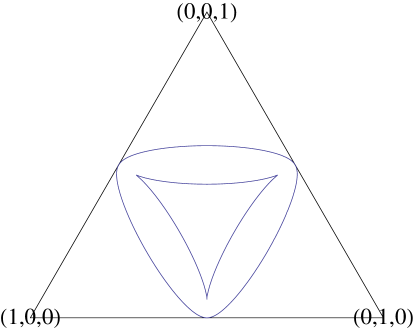
Next, we compute the inverse Fourier transforms at the points of the intersection of the zero set of $H$ with the unit torus. It is easily seen that these consist of $\pm(1,1,1)$ along with a two-dimensional set of smooth points, where $\nabla H$ is nonvanishing; we denote the smooth set by ${\cal V}$. Because the degree of $\overline{H}$ is 3 at $\pm(1,1,1)$ and 1 at any point of ${\cal V}$, the inverse Fourier transform will have homogeneous degree 0 at $\pm(1,1,1)$ and $-2$ at smooth points.

The IFT at $(1,1,1)$ is computed by an elliptic integral. It is nonvanishing on the entire interior of $K^{*}$, varying over the annular region and remaining constant on the facet. While everything else in this example can easily be verified, this computation is not routine and will be detailed in forthcoming work [2]. The role of the contribution from $(-1,-1,-1)$ is to double the contribution to $a_{v}$ from $(1,1,1)$ when the parity of the integer vector $v$ is even and kill it when the parity is odd.

Finally, to put this all together, we check the hypotheses of Corollary 5.9. In fact, hypothesis $(i)$ of Corollary 5.9 is guaranteed whenever the coefficients of $F$ are bounded. To check hypothesis $(ii)$, we need only check that only finitely many points of ${\cal V}$ have a given logarithmic gradient. This is true with the exception of the projective directions $(1,1,0),(1,0,1)$ and $(0,1,1)$, which are the midpoints of the sides of the triangle and are on the outer boundary of the annular region. Therefore, the hypotheses are satisfied over the interior of $K^{*}$.

Summarizing: for $v$ in the facet, $W(v)=\{\pm(1,1,1)\}$, while for $v$ in the annular region, $W(v)$ is equal to the union of $\{\pm(1,1,1)\}$ with a finite set of points on the unit torus where $H$ vanishes but its gradient does not. This completes the verification of hypothesis $(ii)$.

We conclude that $K^{\dagger}=K^{*}$ is everything inside the outer blue boundary in Figure 13. Outside $K^{*}$ there is exponential decay. In the annular region, as $v\to\infty$ with $v/|v|$ tending to $\hat{v}$ and the parity of $v$ remaining even, the coefficient $a_{v}$ tends to a function $\Phi(\hat{v})$ given by an elliptic integral. If $\hat{v}$ is in the facet, $a_{v}$ tends to a constant; due to the three-fold symmetry, the constant must be $1/3$.

In general

In general there is a one-parameter family of curves, the foregoing example being a generic instance. The coefficients of the $8\times 8$ array are rational functions of $a_{0},b_{0},a_{1}$ and $a_{2}$; to get rid of subscripts, we denote these respectively by $a,b,c,d$. Computing the characteristic polynomial and factoring yields $P_{1}P_{2}$ with

$$P_{1} = (C_{1}+C_{2})(x^{2}y^{2}z^{2}-1)-C_{1}(x^{2}y^{2}+x^{2}z^{2}+y^{2}z^{2}-x^{2}-y^{2}-z^{2})$$

$$\;\;\;\;-C_{2}(x^{2}y^{2}+x^{2}z^{2}+x^{2}y^{2}+y^{2}z^{2}+x^{2}z^{2}+y^{2}z^{2}-xy-xz-yz)$$

$$C_{1} := ab^{3}cd$$

$$C_{2} := b^{6}+c^{6}+3ac^{4}d+3a^{2}c^{2}d^{2}+2ab^{3}cd+2b^{3}c^{3}+a^{3}d^{3}\,.$$

In a neighborhood of the values $a=b=1,c=2,d=3$ from the worked example, the same argument shows there must be a factor of $P_{2}$ in the numerator, so that the reduced generating function is rational with denominator $P_{1}$; by analytic continuation, this is true for all parameter values.

Recentering at $(1,1,1)$ via the substitution $x=1+X,y=1+Y,z=1+Z$ and taking the lowest degree homogeneous term at the origin yields

$$\overline{H}=(1-\theta)(X^{2}Y+X^{2}Z+Y^{2}X+Y^{2}Z+Z^{2}X+Z^{2}Y)+(2+6\theta)XYZ$$

where $\theta:=C_{1}/(C_{1}+C_{2})$. We rewrite this as a constant times

$$X^{2}Y+X^{2}Z+Y^{2}X+Y^{2}Z+Z^{2}X+Z^{2}Y+\lambda XYZ$$ (26)

where

$$\lambda = \frac{2+6\theta}{1-\theta}$$

$$= 2\,{\frac{2\,{c}^{3}{b}^{3}+6\,acd{b}^{3}+{c}^{6}+3\,a{c}^{4}d+3\,{a}^{2}{c}^{2}{d}^{2}+{a}^{3}{d}^{3}+{b}^{6}}{{a}^{3}{d}^{3}+{b}^{6}+3\,{a}^{2}{c}^{2}{d}^{2}+3\,a{c}^{4}d+2\,acd{b}^{3}+{c}^{6}+2\,{c}^{3}{b}^{3}}}\,.$$

As $a,b,c,d$ vary over positive reals, the quantity $\lambda$ varies over the half-open interval $(2,3]$. It reaches its maximum value when $a=1,b=2\sqrt{3},c=\sqrt{3}$ and $d=9$ (or at any scalar multiple of this 4-tuple of values) and corresponds to the initial conditions (24).

When $\lambda=3$, the polynomial $\overline{H}$ factors as $(X+Y+Z)(XY+XZ+YZ)$ and when $\lambda=2$ it factors as $(X+Y)(X+Z)(Y+Z)$. However, for $2<\lambda<3$ this polynomial is irreducible with the zero set looking like a cone together with a ruffled collar. Figure 14 shows two examples: on the left $\lambda=5/2$ and on the right $\lambda=66/31$, a value much nearer to 2 which is the value from the example with $a=b=1,c=2$ and $d=3$.

Figure 14: As $\lambda\to 2$ the collar becomes more ruffled

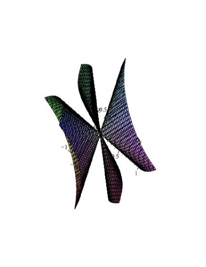
At $\lambda=3$ the dual shape is, as we have seen, the inscribed circle; the facet region in this case is degenerate, having shrunk to a point. As $\lambda$ decreases from $3$ to $2$, the circle deforms to look more like an inscribed triangle and the facet grows, approaching the outer curve.

6 Ising model

In this section we will show how the Ising-Y-Delta move for the Ising model is a special case of the hexahedron recurrence. We begin by recalling the definition of the Ising model. Let $G=(V,E)$ be a finite graph with $c\,:\,E\to\mathbb{R}_{+}$ a positive weight function on edges. The Ising model is a probability measure $\mu$ on the configuration space $\Omega=\{\pm 1\}^{V}$. A configuration of spins $\sigma\in\Omega$ has probability

$$\mu(\sigma)=\frac{1}{Z}\prod_{e=\{v,v^{\prime}\}\in E}c(e)^{(1+\sigma(v)\sigma(v^{\prime}))/2},$$ (27)

where the product is over all edges in $E$ and the partition function $Z$ is the sum of the unweighted probabilities $\prod c(e)^{(1+\sigma(v)\sigma(v^{\prime}))/2}$ over all configurations $\sigma$. In other words, the probability of a configuration is proportional to the product of the edge weights of those edges where the spins are equal. The Ising model originated as a thermodynamical ensemble with energy function $H(\sigma)=-\sum_{e}\sigma(v)\sigma(v^{\prime})J(e)$: take $J(e)=(T/2)\log c(e)$ where $T$ is Boltzmann’s constant times the temperature.

6.1 Ising-Y-Delta move

The Ising-Y-Delta move on the weighted graph $G=(V,E,c)$ transforms the graph the same way as does the Y-Delta move for electrical networks but transforms the edge weights differently. The transformation is depicted in Figure 15.

Figure 15: The Y-Delta move.

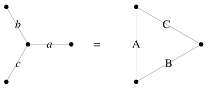
As is apparent, it converts a Y-shape to a triangle shape, or vice versa. The old weights $(a,b,c)$ are replaced by weights $(A,B,C)$ defined by

$$A = \sqrt{\frac{(abc+1)(a+bc)}{(b+ac)(c+ab)}}$$ (28)

$$B = \sqrt{\frac{(abc+1)(b+ac)}{(a+bc)(c+ab)}}$$ (29)

$$C = \sqrt{\frac{(abc+1)(c+ab)}{(a+bc)(b+ac)}}.$$ (30)

Lemma 6.1.

Equations (28)–(30) are the unique positive solution to

$$[abc+1:a+bc:b+ac:c+ab]=[ABC:A:B:C]$$ (31)

Referring to Figure 15, if the Ising edge weights satisfy (31) then the Ising-Y-Delta move preserves the measure $\mu$ in the sense that there is a bijection on the space of configurations of the graph $G$ and the graph $G^{\prime}$ obtained from $G$ by applying the Ising-Y-Delta transformation which maps the Ising measure $\mu_{G}$ to the Ising measure $\mu_{G^{\prime}}$. The same is true with boundary conditions.

Proof.

The first statement is a calculation. For the second statement, observe that up to a global sign there are four possible assignments of spins to the three vertices of the triangle (the three outer vertices of the Y). For example if the three spins are $+++$ then the edges of the triangle contribute weight $ABC$ to the weight of the configuration; in this case for the Y graph the central spin is either $+$, in which case the contribution is abc, or $-$, in which case the contribution is $1$. Similarly the contributions for the $++-,+-+$, and $-++$ configuration are $C,B,A$ and $c+ab,b+ac,a+bc$, respectively. As long as the quadruple of local contributions from the $Y$ is proportional to that of the $\Delta$ the measures will be the same for the two graphs. ∎

6.2 Kashaev’s relation

Suppose that $\mathcal{G}=(V,E)$ is any planar graph with positive weight function $c:E\to\mathbb{R}^{+}$. Kashaev [11] showed how the space of edge weights for the Ising model on $\mathcal{G}$ can be parametrized differently using weights on the vertices and faces, rather than the edges. This parametrization has the advantage that the Y-Delta move has a simpler form in these new coordinates. Let $f$ be any positive function on vertices and faces of $\mathcal{G}$. On each edge $e=vv^{\prime}$ with adjacent faces $F,F^{\prime}$, let $b(e)$ be the ratio $b(e)=\frac{f(v)f(v^{\prime})}{f(F)f(F^{\prime})}.$ Kashaev associated the weight function $w$ with $f$ where $w(e)$ is the positive solution of $(w-1/w)^{2}/4=b(e)$.

Lemma 6.2 ([11]).

Let $f_{0},\dots,f_{7}$ be the values at the faces and vertices involved in a Y-Delta transformation, as in Figure 16. Then we have the identity

$$f_{0}^{2}f_{7}^{2}+f_{1}^{2}f_{4}^{2}+f_{2}^{2}f_{5}^{2}+f_{3}^{2}f_{6}^{2}-2(f_{1}f_{2}f_{4}f_{5}+f_{1}f_{4}f_{3}f_{6}+f_{2}f_{3}f_{5}f_{6})\\ -2f_{0}f_{7}(f_{1}f_{4}+f_{2}f_{5}+f_{3}f_{6})-4(f_{0}f_{4}f_{5}f_{6}+f_{7}f_{1}f_{2}f_{3})=0\,.$$ (32)

Figure 16: The $f$ variables in the Y-Delta move.

Proof.

This is easy enough to check from (28)-(30), with $\frac{(a-1/a)^{2}}{4}=\frac{f_{0}f_{1}}{f_{5}f_{6}}$, etc. ∎

We note that the remarkable formula (32) has another origin: it is the algebraic identity relating the principal minors of a symmetric matrix, as follows.

Lemma 6.3.

Let $M$ be an $n\times n$ matrix and for $S\subset\{1,2,3\}$ let $M_{S}$ be the principal minor of $M$ which is the determinant of the matrix obtained from $M$ by removing rows and columns indexed by $S$. Then for the $8$ subsets of $S$ the identity (32) holds with

$$f_{0}=M_{\phi},f_{1}=M_{1},f_{2}=M_{2},f_{3}=M_{3},f_{4}=-M_{23},f_{5}=-M_{13},f_{6}=-M_{12},f_{7}=-M_{123}\,.$$

For an explanation of this fact, as well as the analogous facts for the Hirota and Miwa equations, see [10].

Proof.

One checks this easily for a $3\times 3$ matrix. For an $n\times n$ matrix $M$, recall that Jacobi’s identity relates minors of $M$ with complementary minors of $M^{-1}$:

$$\frac{M_{S}}{M_{\phi}}=(M^{-1})_{S^{c}}.$$

(In general there is a sign involved but for principal minors this sign is $+1$.) The equation (32) holds for the $3\times 3$ submatrix of $M^{-1}$ indexed by $S$; this implies that it holds for $M$ for the complementary minors. ∎

When placed on a lattice, the relation (32) has an interpretation as a recurrence for stepped surfaces. Previously we associated a graph $\Gamma(U)$ with each stepped surface $\partial U$; now we associate another graph ${\Upsilon}(U)$. The vertices of ${\Upsilon}(U)$ are taken to be the even vertices of $\partial U$ and the edges of ${\Upsilon}(U)$ are the diagonals of the faces of $\partial U$ whose endpoints are even. Because every face of $\partial U$ is a quadrilateral, the graph ${\Upsilon}U$ is planar. If $f:\mathbb{Z}^{d}\to\mathbb{R}^{+}$ is a positive function, define edge weight $w(e)$ on an edge $e$ of ${\Upsilon}(U)$ to be the positive solution to $(w-1/w)^{2}/4=b$ where $b=f(v)f(v^{\prime})/(f(u)f(u^{\prime}))$, where $e=\{v,v^{\prime}\}$ and where $u$ and $u^{\prime}$ are the other two vertices of the face of $\partial U$ on which $e$ lies. The previous lemma results in the following lattice relation, known as Kashaev’s difference equation.

Lemma 6.4.

Let $U\subseteq U^{\prime}$ be stepped solids differing by a single cube.

1. The graph ${\Upsilon}(U^{\prime})$ differs from ${\Upsilon}(U)$ by a Y-Delta move: Y to Delta if the bottom vertex of the added cube was even and Delta to Y otherwise.

2. If $e$ is a weight function on the edges of ${\Upsilon}(U)$, extended by the Ising-Y-Delta relations to the edges of ${\Upsilon}(U^{\prime})$, and if $f$ is a function on the vertices of $\mathbb{Z}^{d}$ inducing $e$ on the edges of ${\Upsilon}(U)$ and ${\Upsilon}(U^{\prime})$ then at the eight vertices of the added cube, $f$ satisfies the relations (3).

$\hfill\Box$

Kashaev’s relation is almost a recurrence: $f_{(123)}$ is determined from the other seven values up to the choice of root of a quadratic equation. It turns out there is a canonical choice.

Proposition 6.5.

Let

$$X=\sqrt{ff_{(23)}+f_{(2)}f_{(3)}},\quad Y=\sqrt{ff_{(13)}+f_{(1)}f_{(3)}},\quad Z=\sqrt{ff_{(12)}+f_{(1)}f_{(2)}}.$$

Then the recurrence (3) can be written

$$X_{(1)} = \frac{f_{(1)}X+YZ}{f}$$ (33)

$$Y_{(2)} = \frac{f_{(2)}Y+XZ}{f}$$ (34)

$$Z_{(3)} = \frac{f_{(3)}Z+XY}{f}$$ (35)

$$f_{(123)} = \frac{2f_{(1)}f_{(2)}f_{(3)}+ff_{(1)}f_{(23)}+ff_{(2)}f_{(13)}+ff_{(3)}f_{(12)}+2XYZ}{f^{2}}\,.$$ (36)

$\hfill\Box$

The proof is a simple verification.

6.3 Embedding Kashaev’s recurrence in the hexahedron recurrence

The proof of all results in this section are straightforward substitutions and are omitted.

Proposition 6.6.

Suppose $f:{\mathbb{Z}^{3}_{1/2}}\to\mathbb{C}$ satisfies the following relation for integer $(i,j,k)$:

$$f(i+1/2,j+1/2,k)^{2} = f(i,j,k)f(i+1,j+1,k)+f(i,j+1,k)f(i+1,j,k)$$

$$f(i+1/2,j,k+1/2)^{2} = f(i,j,k)f(i+1,j,k+1)+f(i,j,k+1)f(i+1,j,k)$$

$$f(i,j+1/2,k+1/2)^{2} = f(i,j,k)f(i,j+1,k+1)+f(i,j,k+1)f(i,j+1,k)\,.$$

Then $f$ satisfies the Kashaev relation (3) at integer points if $f$ satisfies the hexahedron relations (4)–(7), where as usual we interpret $h=f$, $h^{(x)}=f_{(0,1/2,1/2)}$, $h^{(y)}=f_{(1/2,0,1/2)}$ and $h^{(z)}=f_{(1/2,1/2,0)}$. $\hfill\Box$

We obtain the Ising-Y-Delta recurrence as a corollary.

Corollary 6.7.

Suppose the initial conditions for $f$ at the vertices of a stepped surface $\partial U$ are real and positive. Define $f$ on the $z$-faces of the stepped surface by

$$f(i+1/2,j+1/2,k):=\sqrt{f(i,j,k)f(i+1,j+1,k)+f(i,j+1,k)f(i+1,j,k)}$$

and similarly for the $x$- and $y$-faces, always taking the positive square root. Then the values produced by the hexahedron recurrence at all points above the stepped surface, restricted to integer points, yield the Ising-Y-Delta recurrence. $\hfill\Box$

Remark.

Another way to say this is that the equation (32) is a special case of (12). Setting $a_{1}=\sqrt{a_{5}a_{6}+a_{0}a_{7}},a_{2}=\sqrt{a_{4}a_{6}+a_{0}a_{8}}$ and $a_{3}=\sqrt{a_{4}a_{5}+a_{0}a_{9}}$, the recurrence (12) becomes (32) after relabelling variables to correspond to the same geometric positions: $f_{0}=a_{0},f_{1}=a_{4},f_{4}=a_{7}$ etc.

As in the dimer case let us consider initial conditions on the stepped surface defined by $0\leq i+j+k\leq 2$ (take $U$ to be the lattices cubes lying entirely within $\{(x,y,z):x+y+z\leq 2\}$). Recall that $\Gamma(U)$ was the 4-6-12 graph. It is easy to see that ${\Upsilon}(U)$ is the regular triangulation. Indeed, there is a vertex of ${\Upsilon}(U)$ at the center of each dodecagon of $\Gamma(U)$ and an edge of ${\Upsilon}(U)$ connecting dodecagons that share a quadrilateral neighbor. The function $f$ now takes values on the vertices and faces of this triangulation and the $X,Y,Z$ values lie on the three directions of edges. Starting with initial data of the $f$ values on $\{0\leq i+j+k\leq 2\}$, one can determine $X_{i,j,k},Y_{i,j,k},Z_{i,j,k}$ on the set $i+j+k=0$. From (33)–(35) one can then determine the values of $X,Y,Z$ on $i+j+k=1$; then from (36) one can determine the values of $f$ on $i+j+k=3$, and so on; in this way one determines $X,Y,Z,f$ on all planes $i+j+k\geq 0$. Theorem 4.1 has the following consequence for the $f_{i,j,k}$.

Theorem 6.8.

$f_{i,j,k}$ is a Laurent polynomial in the initial variables $\{f_{i,j,k}\}_{0\leq i+j+k\leq 2}$ and $\{X_{i,j,k},Y_{i,j,k},Z_{i,j,k}\}_{i+j+k=0}$. The $X,Y,Z$ variables only appear with power $1$.

Proof.

Let $\{a_{ijk}\}$ denote the initial conditions for the hexahedron recurrence (before specialization), thus $f_{ijk}=a_{ijk}$ for $0\leq i+j+k\leq 2$. Take a monomial $M$ in the Laurent expansion of $a_{i,j,k}$. Let $a_{0}$ be a quadrilateral variable; it occurs in $M$ with exponent in $[-2,2].$

There are several cases to consider. If $a_{0}$ occurs with power $2$, we can replace it with $a_{1}a_{3}+a_{2}a_{4}$ where $a_{1},a_{2},a_{3},a_{4}$ are the four faces in cyclic order adjacent to $a_{0}$. Then the monomial $M$ becomes a sum of two monomials not involving $a_{0}$.

If $a_{0}$ appears with degree $-1$, there is another monomial $M^{\prime}$ of $a_{i,j,k}$ which pairs with it, in the sense that $M/M^{\prime}=\frac{a_{1}a_{3}}{a_{2}a_{4}}$ (these two monomials correspond to the two possible configurations of double-dimers which have three edges lying along the quad face at $a_{0}$, and use the same two edges joining the quad face to adjacent faces: as in line $2$ or Figure 12). The sum of these two monomials is, up to monomial factors $M^{*}$ not involving $a_{0}$, $M+M^{\prime}=M^{*}(a_{1}a_{3}+a_{2}a_{4})/a_{0}=M^{*}a_{0}.$ Upon replacing $a_{0}$ by $\sqrt{a_{1}a_{3}+a_{2}a_{4}}$ this now becomes a monomial in which $a_{0}=\sqrt{a_{1}a_{3}+a_{2}a_{4}}$ occurs with power $+1$.

If $a_{0}$ which appears in $M$ with degree $-2$, there are two other monomials $M^{\prime},M^{\prime\prime}$, which in the appropriate order have the ratios $\displaystyle{[2:\frac{a_{1}a_{3}}{a_{2}a_{4}}:\frac{a_{2}a_{4}}{a_{1}a_{3}}]}$ (these correspond to the three possible configurations of double-dimers which have four edges lying along the quad face at $a_{0}$, as in the first line of Figure 12). The sum of these is

$$M+M^{\prime}+M^{\prime\prime}=M^{*}\frac{\displaystyle{2+\frac{a_{1}a_{3}}{a_{2}a_{4}}+\frac{a_{2}a_{4}}{a_{1}a_{3}}}}{a_{0}^{2}}=M^{*}\frac{a_{0}^{2}}{a_{1}a_{2}a_{3}a_{4}}$$

and upon the substitution $a_{0}^{2}=a_{1}a_{3}+a_{2}a_{4}$ this is a sum of two monomials not involving $a_{0}$.

Once all these substitutions (and groupings) are done, $a_{0}$ only appears in the numerator and has degree $1$ or $0$. We can similarly regroup terms for all the other quad variables: since no two quad faces are adjacent the groupings “commute” in the sense that they can be done in any order.

After regrouping all quad variables, we see that $f_{i,j,k}$ (the specialization of $a_{i,j,k}$) is a Laurent polynomial, with positive coefficients, in the initial variables $f,X,Y,Z$, and with the $X,Y,Z$ (the quad variables) appearing in the numerator only and of degree $0$ or $1$. ∎

6.4 Open question

What are the natural combinatorial structures counted by the monomials in $f_{i,j,k}$? Using Proposition 6.6 it appears possible (although we have not succeeded) to get an interpretation of the monomials in the expansion of $f_{i,j,k}$ in terms of collections of double-dimer covers of $\Gamma_{i+j+k}$.

Note however that when we apply the substitutions of the proof of that proposition, it is possible that the new monomials are not distinct, and combine to make monomials of $f_{i,j,k}$ in other ways. This is already true of $a_{1,1,1},$ in which $9$ monomials collapse into a single monomial of $f_{1,1,1}$.

6.5 Solving the recurrence for spatially isotropic initial conditions

There is a three-parameter family of initial conditions for which $f_{(i,j,k)}=f_{i+j+k}$ only depends on $i+j+k$: choose values $f_{0}=a,f_{1}=b$ and $f_{2}=c$ arbitrarily and set the initial $X$, $Y$ and $Z$ variables all equal to $\sqrt{ac+b^{2}}$. The recurrence (3) can be solved for $f_{n+3}$ as a function of $f_{n},f_{n+1},f_{n+2}$, giving

$$f_{n+3}=\frac{2f_{n+1}^{3}+3f_{n}f_{n+2}f_{n+1}+2\sqrt{f_{n+1}^{6}+3f_{n}f_{n+2}f_{n+1}^{4}+3f_{n}^{2}f_{n+2}^{2}f_{n+1}^{2}+f_{n}^{3}f_{n+2}^{3}}}{f_{n}^{2}}\,.$$

This can be solved explicitly for $f_{n}$ as a function of $a,b$ and $c$. Letting $R:=ac/b^{2}$ and

$$S=\frac{2(R+1)^{3/2}+3R+2}{R^{2}}$$

gives

$$f_{n}=a^{1-n}b^{n}R^{\left\lfloor\frac{n^{2}}{4}\right\rfloor}S^{\left\lfloor\frac{1}{4}(n-1)^{2}\right\rfloor}\,,$$ (37)

or in terms of alternating parity,

$$f_{2n} = a^{1-2n}b^{2n}R^{n^{2}}S^{n^{2}-n}$$ (38)

$$f_{2n+1} = a^{-2n}b^{2n+1}R^{n^{2}+n}S^{n^{2}}\,.$$ (39)

For example when $a=1,b=\sqrt{3},c=9$ we have $R=S=3$ and

$$f_{i,j,k}=f_{i+j+k}=3^{(i+j+k)^{2}/2}.$$ (40)

One can likewise compute limit shapes for $f_{i,j,k}$ as we did for $a_{i,j,k}$ although without a probabilistic interpretation their meaning is dubious.

References

- [1] Y. Baryshnikov and R. Pemantle, Asymptotics of multivariate sequences, part III: quadratic points, Adv. Math. 228 (2011), 3127–3206.
- [2] Y. Baryshnikov and R. Pemantle, Elliptic and hyper-elliptic asymptotics of trivariate generating functions with singularities of degree 3 and 4. In preparation.
- [3] G. Carroll, D. Speyer, The cube recurrence, El. J. Comb 11 (2004), research paper 74.
- [4] Y. Colin de Verdière, Réseaux électriques planaires I, Comment. Math. Helv., 69 (1994), 351–374.
- [5] C. Dodgson, Condensation of determinants, being a new and brief method for computing their arithmetical values, Proc. Royal Soc. London, 15 (1866–1867),150–155.
- [6] P. Du, I. Gessel, A. Ionescu, R. Pemantle and J. Propp, The Aztec diamond edge probability generating function, In preparation.
- [7] S. Fomin and A. Zelevinsky, Cluster Algebras, I. J. Amer. Math. Soc. 15 (2002), 497–529.
- [8] S. Fomin, A. Zelevinsky: The Laurent phenomenon. Adv. in Appl. Math. 28 (2002), no. 2, 119 144. arXiv:math/0104241.
- [9] A. B. Goncharov, R. Kenyon, Dimers and Integrability, Ann. ENS.
- [10] A. B. Goncharov, R. Kenyon, Dimers and the Beauville integrable system, in preparation.
- [11] Kashaev, On discrete three-dimensional equations associated with the local Yang-Baxter relation. Lett. Math. Phys. 33 (1996), 389-397
- [12] A. Kennelly, Equivalence of triangles and stars in conducting networks, Elec. World and Engineer, 34 (1899), 413–414.
- [13] R. Kenyon, A. Okounkov, Limit shapes and the complex Burgers equation, Acta Math. Volume 199, Number 2 (2007), 263-302,
- [14] R. Kenyon, J. Propp, D. Wilson, Trees and Matchings. Electron. J. Combin. 7 (1999)
- [15] A. Kuniba, T. Nakanishi, J. Suzuki, T-systems and Y-systems in integrable systems arXiv:1010.1344v3
- [16] A. Lehman, em Wye-delta transformations in probabilistic networks, J. SIAM 11 (1963), 773–805.
- [17] R. Pemantle and M. Wilson, Analytic Combinatorics in Several Variables, Cambridge University Press (2013), to appear.
- [18] T. K. Peterson, D. Speyer An arctic circle theorem for Groves, J. Comb. Theory A Volume 111, Issue 1, July 2005, Pages 137 164.
- [19] D. Speyer, Perfect matchings and the octahedron recurrence. J. Algebraic Combin. 25 (2007), no. 3, 309 348.