Locally Rotationally Symmetric Bianchi Type-I cosmological model in f​(T)𝑓𝑇f(T) gravity: from early to Dark Energy dominated universe

M. E. Rodrigues (a,b)111E-mail address: esialg@gmail.com, I. G. Salako (c)222E-mail address: ines.salako@imsp-uac.org, M. J. S. Houndjo (c)(d)333E-mail address: sthoundjo@yahoo.fr and J. Tossa (c)444E-mail address: joel.tossa@imsp-uac.org,

a  Faculdade de FΓ­sica, Universidade Federal do ParΓ‘, 66075-110, BelΓ©m, ParΓ‘, Brazil
b
  Faculdade de CiΓͺncias Exatas e Tecnologia, Universidade Federal do ParΓ‘ - Campus UniversitΓ‘rio de Abaetetuba, CEP 68440-000, Abaetetuba, ParΓ‘, Brazil

cInstitut de MathΓ©matiques et de Sciences Physiques (IMSP) - 01 BP 613 Porto-Novo, BΓ©nin
dFacultΓ© des Sciences et Techniques de Natitingou - UniversitΓ© de Parakou - BΓ©nin

Abstract

We study the locally rotational symmetry Bianchi type-I dark energy model in the framework of f​(T)𝑓𝑇f(T) theory of gravity, where T𝑇T denotes the torsion scalar. A viable cosmological model is undertaken and the isotropization of this latter is checked, yielding a result that reflects the real evolution of our universe. Moreover, still in the anisotropic optic, a more complicated f​(T)𝑓𝑇f(T) model is obtained from the cosmological reconstruction scheme and the analysis shows that the universe is more anisotropic at the beginning if the terms of higher order in T𝑇T are not considered. This means that the non-linear model should be favoured by observational data.

Pacs numbers: 98.80.-k, 04.50.Kd, 04.20.Jb

1 Introduction

The discovery of the accelerated expansion of the late-time universe gives rise to a wide spectrum of various theories in order to explain this acceleration. In the general gravity (GR) scheme, the dark energy, known to have an exotic property such as negative pressure, is considered to be a first candidate to this acceleration of the universe [1]. Still in this spirit, and as alternatives to the GR, several theories based on the modification of the the curvature scalar have been developed with interesting results. The most important ones are the f​(R)𝑓𝑅f(R) [2]-[5], f​(G)𝑓𝐺f(G) [6]-[10], f​(R,G)𝑓𝑅𝐺f(R,G) [11]-[18], f​(R,𝒯)𝑓𝑅𝒯f(R,\mathcal{T}) [19]-[24], where R𝑅R, G𝐺G and 𝒯𝒯\mathcal{T} are the curvature scalar, the Gauss-Bonnet invariant and the trace of the energy-momentum tensor, respectively.

Nevertheless, there exists another alternative to the dark energy, being the modification of the teleparallel theory equivalent to the GR (TEGR), namely f​(T)𝑓𝑇f(T) theory of gravity, where T𝑇T denotes the torsion scalar. Instead of the Levi-Civita’s connection, as used in the GR and its different modified versions, the connection under consideration in f​(T)𝑓𝑇f(T) is that of Weitzenbok. This theory has been introduced first by Ferraro [26] where they explained the U​Vπ‘ˆπ‘‰UV modifications to GR and also the inflation. Afterwards, Ferraro and Bengochea considered the same models in the context of late cosmology to describe dark energy [27]. Other authors developed various cosmological and gravitational ideas, still in f​(T)𝑓𝑇f(T) theory of gravity. In [28], Tamanini and Boehmer investigate the importance of choosing good tetrads for the study of the field equations of f​(T)𝑓𝑇f(T) gravity. It is important to recall that the use of specific tetrads is extremely crucial of having a reasonable feature in this theory. Note that when the set of tetrads is not suitably chosen, the theory falls into the usual teleparallel one and there will be no reason of why having modified the teleparallel theory. This important scheme of choosing a suitable set of tetrads is also undertaken in this manuscript and presented in the section 333, where it will be observed that the algebraic function f​(T)𝑓𝑇f(T) may be different from the linear form one, the teleparallel action term.

Universe is assumed to be homogeneous and isotropic at large scales. However, this is not the case if local consideration are made. In such a situation, the anisotropic effects that appears should not be described with the use of the common Friedmann-Robertson-Walker (FRW) metric. The simplest of anisotropic models usually used for describing the anisotropic effects are Bianchi type I (BI) spatially homogeneous models whose spatial sections are flat. The advantages in using anisotropic models are that they have significant role in the description of the early stage of the universe [50] and also are extremely useful in obtaining more general cosmological models that the isotropic FRW models. Anisotropy is completely supported in various angle scales by the Differential Microwave Radiometers on NASA’s Cosmic Background Explorer. Speculations indicate that the entire history of the cosmic evolution down to the recombination is hidden in anisotropies and they are conceived to be indicative the matter composing and the geometry of the universe. Important theoretical argument by Misner in 1968 and the modern experimental data defend the existence of anisotropic phase of the universe, which, later, turns into an isotropic one.

Therefore, its quite reasonable to check the isotropization of any anisotropic model able to describe a stage of the evolution history of the universe. At a simple level, the isotropy of the present stage of the universe allows the BI model to be a prime candidate in the study of the possible effects of an anisotropy in the early universe on the current observational data.

Recently, Fadragas et al [40] performed a detailed dynamical analysis of anisotropic scalar-field cosmologies, and in particular of the most significant Kantowski-Sachs, Bianchi I and Bianchi III case, and as conclusion, they found a very rich behaviour, and amongst others the universe can result in isotropized solutions with observables in agreement with observations, such as de Sitter, quintessence-like or stiff-dark energy solutions. Fontanini et al considered the cosmic parallax effect in anisotropic cosmological models described by an axisymmetric homogeneous Bianchi I metric and discuss whether any observation of cosmic parallax would distinguish between different anisotropic evolutions [41]. Still in the framework of anisotropic models, Campanelli et al [42] analysed the magnitude-redshift data of type Ia supernovae included in the Union and Union2 compilations anisotropic Bianchi I cosmological model and in the presence of dark energy fluid anisotropic equation of state and found that the amount of deviation from isotropy of the equation of state of dark energy, the skewness, which should be restricted to the interval (βˆ’0.16;0.12)0.160.12(-0.16;0.12). Also, in order to well understand the notion of β€œreal-time cosmology”, Quercellini et al undertook the real-time measurements of the overall redshift drift and angular separation shift in distant source, which allows the observer to trace the background cosmic expansion and large scale anisotropy, respectively [43, 44].

Following these evident features of the universe, we focus our attention in this work to the Locally Rotationally Symmetric (LRS) BI model which is a special case of BI one. Within this metric and the general field equations give rise to three independent equations. In the sequence, we present the generalisation of the anisotropic model within torsion consideration. As we mentioned above, the isotropization is an important aspect following the evolution history of the universe. This feature is extensively analysed in the framework of LRS-BI model in this work. The final and important point undertaken in this work is the reconstruction of f​(T)𝑓𝑇f(T) model according to the LRS-BI metric. Across all the above studies, two interesting cases are considered. A linear form of the algebraic function and a more complicated case. Our results show that for the linear case, the real evolution of our universe holds whereas, for the more complicated one, the universe presents more anisotropy at the beginning only when the terms of higher order in T𝑇T fade away.

The paper is organized as follows. In Sec. 2 we present the preliminary definitions and equations of motion in f​(T)𝑓𝑇f(T) gravity. The field equations are presented according to the LRS-BI metric in Sec. 3. The Sec. 4 is devoted to the generalisation of the anisotropic models with the torsion and also to the isotropization scheme. A linear case f​(T)=0𝑓𝑇0f(T)=0 is developed in the Sec. 5 and our conclusions are presented in Sec. 6.

2 Preliminary definitions and equations of motion

As mentioned above, we define f​(T)𝑓𝑇f(T) theory within Weitzenkock’s connection where the line element is described by

d​S2=gμ​ν​d​xμ​d​xΞ½,𝑑superscript𝑆2subscriptπ‘”πœ‡πœˆπ‘‘superscriptπ‘₯πœ‡π‘‘superscriptπ‘₯𝜈dS^{2}=g_{\mu\nu}dx^{\mu}dx^{\nu}\;, (1)

gμ​νsubscriptπ‘”πœ‡πœˆg_{\mu\nu} being the components of the metric. One can describe the theory in the spacetime or in the tangent space. This allows to rewrite the line element (1) as follows

d​S2𝑑superscript𝑆2\displaystyle dS^{2} =\displaystyle= gμ​ν​d​xμ​d​xΞ½=Ξ·i​j​θi​θj,subscriptπ‘”πœ‡πœˆπ‘‘superscriptπ‘₯πœ‡π‘‘superscriptπ‘₯𝜈subscriptπœ‚π‘–π‘—superscriptπœƒπ‘–superscriptπœƒπ‘—\displaystyle g_{\mu\nu}dx^{\mu}dx^{\nu}=\eta_{ij}\theta^{i}\theta^{j}\;, (2)
d​xμ𝑑superscriptπ‘₯πœ‡\displaystyle dx^{\mu} =\displaystyle= eiμ​θi,ΞΈi=eΞΌi​d​xΞΌ,superscriptsubscriptπ‘’π‘–πœ‡superscriptπœƒπ‘–superscriptπœƒπ‘–subscriptsuperscriptπ‘’π‘–πœ‡π‘‘superscriptπ‘₯πœ‡\displaystyle e_{i}^{\;\;\mu}\theta^{i}\;,\;\theta^{i}=e^{i}_{\;\;\mu}dx^{\mu}\;, (3)

where Ξ·i​j=d​i​a​g​[1,βˆ’1,βˆ’1,βˆ’1]subscriptπœ‚π‘–π‘—π‘‘π‘–π‘Žπ‘”1111\eta_{ij}=diag[1,-1,-1,-1] and eiμ​eΞ½i=δνμsuperscriptsubscriptπ‘’π‘–πœ‡subscriptsuperscriptπ‘’π‘–πœˆsubscriptsuperscriptπ›Ώπœ‡πœˆe_{i}^{\;\;\mu}e^{i}_{\;\;\nu}=\delta^{\mu}_{\nu} or eiμ​eΞΌj=Ξ΄ijsuperscriptsubscriptπ‘’π‘–πœ‡subscriptsuperscriptπ‘’π‘—πœ‡subscriptsuperscript𝛿𝑗𝑖e_{i}^{\;\;\mu}e^{j}_{\;\;\mu}=\delta^{j}_{i}. We also express the square root of the metric determinant by βˆ’g=det[eΞΌi]=e𝑔delimited-[]subscriptsuperscriptπ‘’π‘–πœ‡π‘’\sqrt{-g}=\det{\left[e^{i}_{\;\;\mu}\right]}=e and the matrix eΞΌasubscriptsuperscriptπ‘’π‘Žπœ‡e^{a}_{\;\;\mu} are called tetrads and play the crucial role in the dynamic fields of the theory.

By using theses fields, we define the Weitzenbock’s connection as

Γμ​να=eiΞ±β€‹βˆ‚Ξ½eΞΌi=βˆ’eΞΌiβ€‹βˆ‚Ξ½eiΞ±.subscriptsuperscriptΞ“π›Όπœ‡πœˆsuperscriptsubscript𝑒𝑖𝛼subscript𝜈subscriptsuperscriptπ‘’π‘–πœ‡subscriptsuperscriptπ‘’π‘–πœ‡subscript𝜈superscriptsubscript𝑒𝑖𝛼\displaystyle\Gamma^{\alpha}_{\mu\nu}=e_{i}^{\;\;\alpha}\partial_{\nu}e^{i}_{\;\;\mu}=-e^{i}_{\;\;\mu}\partial_{\nu}e_{i}^{\;\;\alpha}\;. (4)

The geometrical objects of the spacetime are then constructed from this connection. The components of the tensor torsion are defined by the antisymmetric part of this connection

Tμ​ναsubscriptsuperscriptπ‘‡π›Όπœ‡πœˆ\displaystyle T^{\alpha}_{\;\;\mu\nu} =\displaystyle= Ξ“Ξ½β€‹ΞΌΞ±βˆ’Ξ“ΞΌβ€‹Ξ½Ξ±=eiα​(βˆ‚ΞΌeΞ½iβˆ’βˆ‚Ξ½eΞΌi).subscriptsuperscriptΞ“π›Όπœˆπœ‡subscriptsuperscriptΞ“π›Όπœ‡πœˆsuperscriptsubscript𝑒𝑖𝛼subscriptπœ‡subscriptsuperscriptπ‘’π‘–πœˆsubscript𝜈subscriptsuperscriptπ‘’π‘–πœ‡\displaystyle\Gamma^{\alpha}_{\nu\mu}-\Gamma^{\alpha}_{\mu\nu}=e_{i}^{\;\;\alpha}\left(\partial_{\mu}e^{i}_{\;\;\nu}-\partial_{\nu}e^{i}_{\;\;\mu}\right)\;. (5)

The components of the contorsion tensor are defined as

Kαμ​νsubscriptsuperscriptπΎπœ‡πœˆπ›Ό\displaystyle K^{\mu\nu}_{\;\;\;\;\alpha} =\displaystyle= βˆ’12​(TΞ±ΞΌβ€‹Ξ½βˆ’TΞ±Ξ½β€‹ΞΌβˆ’Tαμ​ν).12subscriptsuperscriptπ‘‡πœ‡πœˆπ›Όsubscriptsuperscriptπ‘‡πœˆπœ‡π›Όsuperscriptsubscriptπ‘‡π›Όπœ‡πœˆ\displaystyle-\frac{1}{2}\left(T^{\mu\nu}_{\;\;\;\;\alpha}-T^{\nu\mu}_{\;\;\;\;\alpha}-T_{\alpha}^{\;\;\mu\nu}\right)\;. (6)

In order to make more clear the definition of the scalar equivalent to the curvature scalar of RG, we first define a new tensor Sαμ​νsuperscriptsubscriptπ‘†π›Όπœ‡πœˆS_{\alpha}^{\;\;\mu\nu}, constructed from the components of the tensors torsion and contorsion as

Sαμ​νsuperscriptsubscriptπ‘†π›Όπœ‡πœˆ\displaystyle S_{\alpha}^{\;\;\mu\nu} =\displaystyle= 12​(Kαμ​ν+δαμ​TΞ²Ξ²β€‹Ξ½βˆ’Ξ΄Ξ±Ξ½β€‹Tββ​μ).12superscriptsubscriptπΎπ›Όπœ‡πœˆsubscriptsuperscriptπ›Ώπœ‡π›Όsubscriptsuperscriptπ‘‡π›½πœˆπ›½subscriptsuperscriptπ›Ώπœˆπ›Όsubscriptsuperscriptπ‘‡π›½πœ‡π›½\displaystyle\frac{1}{2}\left(K_{\;\;\;\;\alpha}^{\mu\nu}+\delta^{\mu}_{\alpha}T^{\beta\nu}_{\;\;\;\;\beta}-\delta^{\nu}_{\alpha}T^{\beta\mu}_{\;\;\;\;\beta}\right)\;. (7)

We can now define the torsion scalar by the following contraction

T=Tμ​να​Sαμ​ν.𝑇subscriptsuperscriptπ‘‡π›Όπœ‡πœˆsubscriptsuperscriptπ‘†πœ‡πœˆπ›Ό\displaystyle T=T^{\alpha}_{\;\;\mu\nu}S^{\;\;\mu\nu}_{\alpha}\;. (8)

The action of the theory is defined by generalizing the Teleparallel theory, as

S=∫[T+f​(T)+β„’M​a​t​t​e​r]​e​d4​x.𝑆delimited-[]𝑇𝑓𝑇subscriptβ„’π‘€π‘Žπ‘‘π‘‘π‘’π‘Ÿπ‘’superscript𝑑4π‘₯\displaystyle S=\int\left[T+f(T)+\mathcal{L}_{Matter}\right]ed^{4}x\;. (9)

Here, f​(T)𝑓𝑇f(T) denotes an algebraic function of the torsion scalar T𝑇T. Making the functional variation of the action (9) with respect to the tetrads, we get the following equations of motion [45, 46, 47]

SΞΌΞ½β€‹Οβ€‹βˆ‚ΟT​fT​T+[eβˆ’1​eΞΌiβ€‹βˆ‚Ο(e​eiα​Sαν​ρ)+Tλ​μα​Sαν​λ]​(1+fT)+14​δμν​(T+f)=4​π​𝒯μν,subscriptsuperscriptπ‘†πœˆπœŒπœ‡subscriptπœŒπ‘‡subscript𝑓𝑇𝑇delimited-[]superscript𝑒1subscriptsuperscriptπ‘’π‘–πœ‡subscriptπœŒπ‘’subscriptsuperscript𝑒𝛼𝑖subscriptsuperscriptπ‘†πœˆπœŒπ›Όsubscriptsuperscriptπ‘‡π›Όπœ†πœ‡subscriptsuperscriptπ‘†πœˆπœ†π›Ό1subscript𝑓𝑇14subscriptsuperscriptπ›Ώπœˆπœ‡π‘‡π‘“4πœ‹subscriptsuperscriptπ’―πœˆπœ‡\displaystyle S^{\;\;\nu\rho}_{\mu}\partial_{\rho}Tf_{TT}+\left[e^{-1}e^{i}_{\mu}\partial_{\rho}\left(ee^{\;\;\alpha}_{i}S^{\;\;\nu\rho}_{\alpha}\right)+T^{\alpha}_{\;\;\lambda\mu}S^{\;\;\nu\lambda}_{\alpha}\right]\;(1+\;f_{T})+\frac{1}{4}\delta^{\nu}_{\mu}\;(T+f)=4\pi\mathcal{T}^{\nu}_{\mu}\;, (10)

where 𝒯μνsubscriptsuperscriptπ’―πœˆπœ‡\mathcal{T}^{\nu}_{\mu} is the energy momentum tensor, fT=d​f​(T)/d​Tsubscript𝑓𝑇𝑑𝑓𝑇𝑑𝑇f_{T}=df(T)/dT and fT​T=d2​f​(T)/d​T2subscript𝑓𝑇𝑇superscript𝑑2𝑓𝑇𝑑superscript𝑇2f_{TT}=d^{2}f(T)/dT^{2}. By setting f​(T)=a0𝑓𝑇subscriptπ‘Ž0f(T)=a_{0}, a0subscriptπ‘Ž0a_{0} being a constant, the equations of motion (10) are exactly that of the Teleparallel theory with a cosmological constant, and this is dynamically equivalent to the GR. We see from this that the equations clearly depend on the choice made for the set of tetrads [48].

The energy momentum tensor incorporates the interaction of the gravitational field with the matter ones and is defined as

𝒯μν=d​i​a​g​(1,βˆ’Ο‰x,βˆ’Ο‰y,βˆ’Ο‰z)​ρ.subscriptsuperscriptπ’―πœˆπœ‡π‘‘π‘–π‘Žπ‘”1subscriptπœ”π‘₯subscriptπœ”π‘¦subscriptπœ”π‘§πœŒ\displaystyle\mathcal{T}^{\,\nu}_{\mu}=diag\left(1,-\omega_{x},-\omega_{y},-\omega_{z}\right)\rho\;. (11)

Here, Ο‰isubscriptπœ”π‘–\omega_{i} (i=x,y,z𝑖π‘₯𝑦𝑧i=x,y,z) are the parameters of equations of state related to the pressures pxsubscript𝑝π‘₯p_{x}, pysubscript𝑝𝑦p_{y} and pzsubscript𝑝𝑧p_{z}.

3 Field equations for LRS Bianchi type-I model

Let us first establish the equations of motion of a set of diagonal tetrads using the Cartesian coordinate metric, for describing LRS Bianchi type-I model. The LRS Bianchi type-I metric reads

d​S2=d​t2βˆ’A2​(t)​d​x2βˆ’B2​(t)​(d​y2+d​z2),𝑑superscript𝑆2𝑑superscript𝑑2superscript𝐴2𝑑𝑑superscriptπ‘₯2superscript𝐡2𝑑𝑑superscript𝑦2𝑑superscript𝑧2dS^{2}=dt^{2}-A^{2}(t)dx^{2}-B^{2}(t)\left(dy^{2}+dz^{2}\right)\,, (12)

Let us choose the following set of diagonal tetrads related to the metric (57)

[eΞΌa]=d​i​a​g​[1,A,B,B].delimited-[]subscriptsuperscriptπ‘’π‘Žπœ‡π‘‘π‘–π‘Žπ‘”1𝐴𝐡𝐡\displaystyle\left[e^{a}_{\;\;\mu}\right]=diag\left[1,A,B,B\right]\;. (13)

The determinant of the matrix (13) is e=A​B2𝑒𝐴superscript𝐡2e=AB^{2}. The components of the torsion tensor (5) for the tetrads (13) are given by

T  011=AΛ™A,T  022=BΛ™B,,T  033=BΛ™B,\displaystyle T^{1}_{\;\;01}=\frac{\dot{A}}{A}\,,\,T^{2}_{\;\;02}=\frac{\dot{B}}{B}\,,\,,\,T^{3}_{\;\;03}=\frac{\dot{B}}{B}\;, (14)

and the non null components of the corresponding contorsion tensor are

K    101=AΛ™A,K    202=BΛ™B,,K    303=BΛ™B.\displaystyle K^{01}_{\;\;\;\;1}=\frac{\dot{A}}{A}\,,\,K^{02}_{\;\;\;\;2}=\frac{\dot{B}}{B}\,,\,,\,K^{03}_{\;\;\;\;3}=\frac{\dot{B}}{B}\;. (15)

The components of the tensor Sαμ​νsuperscriptsubscriptπ‘†π›Όπœ‡πœˆS_{\alpha}^{\;\;\mu\nu}, in (7), are given by

S1  10=BΛ™B,S2  20=12​(AΛ™A+BΛ™B),S3  30=12​(AΛ™A+BΛ™B).formulae-sequencesuperscriptsubscript𝑆110˙𝐡𝐡formulae-sequencesuperscriptsubscript𝑆22012˙𝐴𝐴˙𝐡𝐡superscriptsubscript𝑆33012˙𝐴𝐴˙𝐡𝐡\displaystyle S_{1}^{\;\;10}=\frac{\dot{B}}{B}\,,\,S_{2}^{\;\;20}=\frac{1}{2}\left(\frac{\dot{A}}{A}+\frac{\dot{B}}{B}\right)\,,\,S_{3}^{\;\;30}=\frac{1}{2}\left(\frac{\dot{A}}{A}+\frac{\dot{B}}{B}\right)\;. (16)

By using the components (14) and (16), the torsion scalar (8) is given by

T=βˆ’2​(2​A˙​BΛ™A​B+BΛ™2B2).𝑇22˙𝐴˙𝐡𝐴𝐡superscript˙𝐡2superscript𝐡2\displaystyle T=-2\left(2\frac{\dot{A}\dot{B}}{AB}+\frac{\dot{B}^{2}}{B^{2}}\right)\;. (17)

The equations of motion corresponding to LRS Bianchi type-I model are obtained by

16​π​ρ16πœ‹πœŒ\displaystyle 16\pi\;\rho =\displaystyle= (f+T)+4​(1+fT)​[(BΛ™B)2+2​A˙​BΛ™A​B],𝑓𝑇41subscript𝑓𝑇delimited-[]superscript˙𝐡𝐡22˙𝐴˙𝐡𝐴𝐡\displaystyle(f+T)+4\;(1+f_{T})\left[\left(\frac{\dot{B}}{B}\right)^{2}+2\frac{\dot{A}\dot{B}}{AB}\right]\;, (18)
16​π​px16πœ‹subscript𝑝π‘₯\displaystyle 16\pi\;p_{x} =\displaystyle= (f+T)+4​(1+fT)​[BΒ¨B+(BΛ™B)2+A˙​BΛ™A​B]+4​BΛ™B​T˙​fT​T,𝑓𝑇41subscript𝑓𝑇delimited-[]¨𝐡𝐡superscript˙𝐡𝐡2˙𝐴˙𝐡𝐴𝐡4˙𝐡𝐡˙𝑇subscript𝑓𝑇𝑇\displaystyle(f+T)+4\;(1+f_{T})\left[\frac{\ddot{B}}{B}+\left(\frac{\dot{B}}{B}\right)^{2}+\frac{\dot{A}\dot{B}}{AB}\right]+4\frac{\dot{B}}{B}\dot{T}f_{TT}\;, (19)
16​π​py16πœ‹subscript𝑝𝑦\displaystyle 16\pi\;p_{y} =\displaystyle= (f+T)+2​(1+fT)​[AΒ¨A+BΒ¨B+(BΛ™B)2+3​A˙​BΛ™A​B]+2​(AΛ™A+BΛ™B)​T˙​fT​T,𝑓𝑇21subscript𝑓𝑇delimited-[]¨𝐴𝐴¨𝐡𝐡superscript˙𝐡𝐡23˙𝐴˙𝐡𝐴𝐡2˙𝐴𝐴˙𝐡𝐡˙𝑇subscript𝑓𝑇𝑇\displaystyle(f+T)+2\;(1+f_{T})\left[\frac{\ddot{A}}{A}+\frac{\ddot{B}}{B}+\left(\frac{\dot{B}}{B}\right)^{2}+3\frac{\dot{A}\dot{B}}{AB}\right]+2\left(\frac{\dot{A}}{A}+\frac{\dot{B}}{B}\right)\dot{T}f_{TT}\;, (20)
pysubscript𝑝𝑦\displaystyle p_{y} =\displaystyle= pz.subscript𝑝𝑧\displaystyle p_{z}\,\,\,.

We parametrize it as follows

𝒯μνsubscriptsuperscriptπ’―πœˆπœ‡\displaystyle\mathcal{T}^{\,\nu}_{\mu} =\displaystyle= d​i​a​g​(1,βˆ’Ο‰x,βˆ’Ο‰y,βˆ’Ο‰z)​ρ,π‘‘π‘–π‘Žπ‘”1subscriptπœ”π‘₯subscriptπœ”π‘¦subscriptπœ”π‘§πœŒ\displaystyle diag\left(1,-\omega_{x},-\omega_{y},-\omega_{z}\right)\rho\;, (21)
=\displaystyle= d​i​a​g​(1,βˆ’Ο‰,βˆ’(Ο‰+Ξ΄),βˆ’(Ο‰+Ξ΄))​ρ,π‘‘π‘–π‘Žπ‘”1πœ”πœ”π›Ώπœ”π›ΏπœŒ\displaystyle diag\left(1,-\omega,-(\omega+\delta),-(\omega+\delta)\right)\rho\,, (22)

where ρ𝜌\rho is the energy density of the fluid; px,pysubscript𝑝π‘₯subscript𝑝𝑦p_{x},\;\;p_{y} and pzsubscript𝑝𝑧p_{z} are the pressures and Ο‰x,Ο‰ysubscriptπœ”π‘₯subscriptπœ”π‘¦\omega_{x},\omega_{y} and Ο‰zsubscriptπœ”π‘§\omega_{z} are the directional equation of state (EoS) parameters of the fluid. Now, parametrizing the deviation from isotropy by setting   Ο‰x=Ο‰subscriptπœ”π‘₯πœ”\omega_{x}=\omega and then introducing skewness parameter δ𝛿\delta that is the deviations from Ο‰πœ”Ο‰ respectively on both the y𝑦y and z𝑧z axes. Here Ο‰πœ”Ο‰ and δ𝛿\delta are not necessarily constants and can be functions of the cosmic time t𝑑t.

The equations of motion corresponding to LRS Bianchi type-I model for an anisotropic fluid are obtained by

16​π​ρ16πœ‹πœŒ\displaystyle 16\pi\;\rho =\displaystyle= (f+T)+4​(1+fT)​[(BΛ™B)2+2​A˙​BΛ™A​B],𝑓𝑇41subscript𝑓𝑇delimited-[]superscript˙𝐡𝐡22˙𝐴˙𝐡𝐴𝐡\displaystyle(f+T)+4\;(1+f_{T})\left[\left(\frac{\dot{B}}{B}\right)^{2}+2\frac{\dot{A}\dot{B}}{AB}\right]\;, (23)
βˆ’16​π​ω​ρ16πœ‹πœ”πœŒ\displaystyle-16\pi\omega\rho =\displaystyle= (f+T)+4​(1+fT)​[BΒ¨B+(BΛ™B)2+A˙​BΛ™A​B]+4​BΛ™B​T˙​fT​T,𝑓𝑇41subscript𝑓𝑇delimited-[]¨𝐡𝐡superscript˙𝐡𝐡2˙𝐴˙𝐡𝐴𝐡4˙𝐡𝐡˙𝑇subscript𝑓𝑇𝑇\displaystyle(f+T)+4(1+f_{T})\left[\frac{\ddot{B}}{B}+\left(\frac{\dot{B}}{B}\right)^{2}+\frac{\dot{A}\dot{B}}{AB}\right]+4\frac{\dot{B}}{B}\dot{T}f_{TT}\;, (24)
βˆ’16​π​(Ο‰+Ξ΄)​ρ16πœ‹πœ”π›ΏπœŒ\displaystyle-16\pi\;(\omega+\delta)\rho =\displaystyle= (f+T)+2​(1+fT)​[AΒ¨A+BΒ¨B+(BΛ™B)2+3​A˙​BΛ™A​B]+2​(AΛ™A+BΛ™B)​T˙​fT​T.𝑓𝑇21subscript𝑓𝑇delimited-[]¨𝐴𝐴¨𝐡𝐡superscript˙𝐡𝐡23˙𝐴˙𝐡𝐴𝐡2˙𝐴𝐴˙𝐡𝐡˙𝑇subscript𝑓𝑇𝑇\displaystyle(f+T)+2\;(1+f_{T})\left[\frac{\ddot{A}}{A}+\frac{\ddot{B}}{B}+\left(\frac{\dot{B}}{B}\right)^{2}+3\frac{\dot{A}\dot{B}}{AB}\right]+2\left(\frac{\dot{A}}{A}+\frac{\dot{B}}{B}\right)\dot{T}f_{TT}\,. (25)

The conservation of the energy-momentum tensor of the fluid parametrized in (22), i.e T;νμ​ν=0T_{;\nu}^{\mu\nu}=0, leads to the following equation:

ρ˙+[AΛ™A​(1+Ο‰)+2​BΛ™B​(1+(Ο‰+Ξ΄))]​ρ=0.Λ™πœŒdelimited-[]˙𝐴𝐴1πœ”2˙𝐡𝐡1πœ”π›ΏπœŒ0\displaystyle\dot{\rho}+\Bigg{[}\frac{\dot{A}}{A}(1+\omega)+2\frac{\dot{B}}{B}(1+(\omega+\delta))\Bigg{]}\;\rho=0\,. (26)

4 Generalized anisotropic models with Torsion and Isotropization

Before determining the parameters Ξ΄,Οπ›ΏπœŒ\delta,\rho and Ο‰πœ”\omega whose involved in the isotropization, we will determine the Hubble parameters in the direction of [x,y,z]π‘₯𝑦𝑧[x,y,z]

Hx=AΛ™A,Hy=BΛ™B,Hz=BΛ™B.formulae-sequencesubscript𝐻π‘₯˙𝐴𝐴formulae-sequencesubscript𝐻𝑦˙𝐡𝐡subscript𝐻𝑧˙𝐡𝐡\displaystyle H_{x}=\frac{\dot{A}}{A}\,,\;\;\,H_{y}=\frac{\dot{B}}{B}\,,\,\;\;H_{z}=\frac{\dot{B}}{B}\,. (27)

The main Hubble parameter is given by

H=13​VΛ™V𝐻13˙𝑉𝑉\displaystyle H=\frac{1}{3}\frac{\dot{V}}{V} =\displaystyle= 13​(AΛ™A+BΛ™B+BΛ™B)13˙𝐴𝐴˙𝐡𝐡˙𝐡𝐡\displaystyle\frac{1}{3}\left(\frac{\dot{A}}{A}+\frac{\dot{B}}{B}+\frac{\dot{B}}{B}\right) (28)
=\displaystyle= 13​(AΛ™A+2​BΛ™B),13˙𝐴𝐴2˙𝐡𝐡\displaystyle\frac{1}{3}\left(\frac{\dot{A}}{A}+2\frac{\dot{B}}{B}\right)\,, (29)

with

V=A​B2,𝑉𝐴superscript𝐡2\displaystyle V=AB^{2}\,, (30)

being the spatial volume of the universe. The rate of expansion is evaluated by anisotropy parameter given as

Ξ”=13β€‹βˆ‘i=13(Hiβˆ’HH)2,Ξ”13subscriptsuperscript3𝑖1superscriptsubscript𝐻𝑖𝐻𝐻2\displaystyle\Delta=\frac{1}{3}\sum^{3}_{i=1}\left(\frac{H_{i}-H}{H}\right)^{2}\,, (31)

where i=(x​y​z)𝑖π‘₯𝑦𝑧i=(\;x\;y\;z\;).

By introducing (29) and (29) into 31, the anisotropy parameter can be written as following

Ξ”=29​H2​(Hxβˆ’Hz)2.Ξ”29superscript𝐻2superscriptsubscript𝐻π‘₯subscript𝐻𝑧2\displaystyle\Delta=\frac{2}{9H^{2}}\left(H_{x}-H_{z}\right)^{2}\,. (32)

The scalar expansion and the shear can be defined as

θ​(t)=AΛ™A+2​BΛ™B,πœƒπ‘‘Λ™π΄π΄2˙𝐡𝐡\displaystyle\theta(t)=\frac{\dot{A}}{A}+2\frac{\dot{B}}{B}\,, (33)
σ​(t)=13​(AΛ™Aβˆ’BΛ™B).πœŽπ‘‘13˙𝐴𝐴˙𝐡𝐡\displaystyle\sigma(t)=\frac{1}{\sqrt{3}}\left(\frac{\dot{A}}{A}-\frac{\dot{B}}{B}\right)\,. (34)

We now we have three linearly independent equations (23)-(26) and five unknown functions A,B,Ο‰,Οπ΄π΅πœ”πœŒA,B,\omega,\rho and δ𝛿\delta. Beside to this, we make use of an additional condition which allows us to choose the volumetric law expansion for solving the system completely. The following two different volumetric expansion laws have been used laws:

V=c1​e3​H0​t,𝑉subscript𝑐1superscript𝑒3subscript𝐻0𝑑\displaystyle V=c_{1}\;e^{3H_{0}t}\,, (35)

where c1subscript𝑐1c_{1} and H0subscript𝐻0H_{0} are two positive constants. Because of the expansion of the universe, one can calculate the deceleration parameter as

q=(dd​t​Hβˆ’1​(t))βˆ’1.π‘žπ‘‘π‘‘π‘‘superscript𝐻1𝑑1q=\left(\frac{d}{dt}H^{-1}(t)\right)-1\,. (36)

Using equations (23), (29), (32) and the identity

Hy2+2​Hx​Hy=3​H2​[1βˆ’Ξ”β€‹(t)2],superscriptsubscript𝐻𝑦22subscript𝐻π‘₯subscript𝐻𝑦3superscript𝐻2delimited-[]1Δ𝑑2\displaystyle H_{y}^{2}+2H_{x}H_{y}=3H^{2}\left[1-\frac{\Delta(t)}{2}\right]\,, (37)

the energy density can be re-written as

3​H2=8​π​ρe​f​f=8​π​(ρ+ρT+ρa​n​i​s),3superscript𝐻28πœ‹subscriptπœŒπ‘’π‘“π‘“8πœ‹πœŒsubscriptπœŒπ‘‡subscriptπœŒπ‘Žπ‘›π‘–π‘ \displaystyle 3H^{2}=8\pi\rho_{eff}=8\pi\left(\rho+\rho_{T}+\rho_{anis}\right)\,, (38)
ρT=βˆ’116​π​[f​(T)+12​H2​fT​(T)],subscriptπœŒπ‘‡116πœ‹delimited-[]𝑓𝑇12superscript𝐻2subscript𝑓𝑇𝑇\displaystyle\rho_{T}=-\frac{1}{16\pi}\left[f(T)+12H^{2}f_{T}(T)\right]\,, (39)
ρa​n​i​s=316​π​H2​Δ​(t)​[1+2​fT​(T)],subscriptπœŒπ‘Žπ‘›π‘–π‘ 316πœ‹superscript𝐻2Δ𝑑delimited-[]12subscript𝑓𝑇𝑇\displaystyle\rho_{anis}=\frac{3}{16\pi}H^{2}\Delta(t)\left[1+2f_{T}(T)\right]\,, (40)

where the subscript `​`​a​n​i​s​"``π‘Žπ‘›π‘–π‘ "``anis" expresses the anisotropic component. By considering the particular case f​(T)=0𝑓𝑇0f(T)=0, one regains the anisotropic LRS-BI model in GR. When one considers the particular case Δ​(t)=0Δ𝑑0\Delta(t)=0 (implying A​(t)β†’B​(t)→𝐴𝑑𝐡𝑑A(t)\rightarrow B(t) in (32)), A​(t)=B​(t)=a​(t)π΄π‘‘π΅π‘‘π‘Žπ‘‘A(t)=B(t)=a(t), and f​(T)𝑓𝑇f(T) is re-obtained in the framework of flat FRW metric. If all the densities are different from zero, one gets a theory that takes into account the anisotropic contribution and the contribution of the terms non-linear in torsion scalar.

In the next section, we will deal with the particular case f​(T)=0𝑓𝑇0f(T)=0, in order to re-obtain the anisotropic dark energy results, as an analogy of the GR.

Now, let us define the necessary condition for an anisotropic model of the universe presenting isotropization. First, let us explain the term β€œisotropization”. The isotropization is the process in which a possible anisotropic universe can adequate with the current observational data, being homogeneous and isotropic; such an universe is said becoming isotropic by the isotropization process. This process is really realised in the inflationary phase and modifies any geometry into an isotropic one and any fluid into an homogeneous one.

The criterion for having the possibility of such a model are known for several years, through the work of Collins and Hawking [49], where they established the following conditions: when taking the limit tβ†’+βˆžβ†’π‘‘t\rightarrow+\infty, one has the function δ​(t)𝛿𝑑\delta(t), in (22), Δ​(t)Δ𝑑\Delta(t), in (32) and M​(t)=σ​(t)/θ​(t)π‘€π‘‘πœŽπ‘‘πœƒπ‘‘M(t)=\sigma(t)/\theta(t)555The functions σ​(t)πœŽπ‘‘\sigma(t) and θ​(t)πœƒπ‘‘\theta(t) are defined in (34) and (33), respectively. tends to zero. This is clear when one makes δ​(t)β†’0→𝛿𝑑0\delta(t)\rightarrow 0 in the definition of energy momentum tensor (22), obtaining a perfect fluid, and when Δ​(t)β†’0→Δ𝑑0\Delta(t)\rightarrow 0 in (32), leading to B​(t)β†’A​(t)→𝐡𝑑𝐴𝑑B(t)\rightarrow A(t), which corresponds to the flat FRW metric in (57).

5 The Linear Case, f​(T)=0𝑓𝑇0f(T)=0

For this work, we have used the model with the exponential expansion given by the relation (35). By using equations (30) and (35), we can obtain:

A​(t)=c1​e3​H0​tB2.𝐴𝑑subscript𝑐1superscript𝑒3subscript𝐻0𝑑superscript𝐡2\displaystyle A(t)=\frac{c_{1}\;e^{3H_{0}\;t}}{B^{2}}\,. (41)

By making use of (24),   (25), (41) after solving (23)-(26), we obtain:

B​(t)=eH0​t​(ΞΊH0+3​λ​eβˆ’3​H0​t)1/3,𝐡𝑑superscript𝑒subscript𝐻0𝑑superscriptπœ…subscript𝐻03πœ†superscript𝑒3subscript𝐻0𝑑13\displaystyle B(t)=e^{H_{0}t}\left(\frac{\kappa}{H_{0}}+3\lambda\;e^{-3H_{0}t}\right)^{1/3}\,, (42)

lead to

A​(t)=c1​eH0​t​(ΞΊH0+3​λ​eβˆ’3​H0​t)βˆ’2/3.𝐴𝑑subscript𝑐1superscript𝑒subscript𝐻0𝑑superscriptπœ…subscript𝐻03πœ†superscript𝑒3subscript𝐻0𝑑23\displaystyle A(t)=c_{1}\;e^{H_{0}t}\left(\frac{\kappa}{H_{0}}+3\lambda e^{-3H_{0}t}\right)^{-2/3}\,. (43)

By introducing (42) and (43) into (29) and (32), we obtain the mean Hubble parameter

H​(t)=H0,𝐻𝑑subscript𝐻0\displaystyle H(t)=H_{0}\,, (44)

and the anisotropy parameter of the expansion as:

Δ​(t)=18​H02​λ2(κ​e3​H0​t+3​H0​λ)2.Δ𝑑18superscriptsubscript𝐻02superscriptπœ†2superscriptπœ…superscript𝑒3subscript𝐻0𝑑3subscript𝐻0πœ†2\displaystyle\Delta(t)=\frac{18\;H_{0}^{2}\;\lambda^{2}}{(\kappa\;e^{3H_{0}t}+3\;H_{0}\;\lambda)^{2}}\,. (45)

By using equation (23), we can obtain the energy density of the fluid as:

ρ1​(t)=3​κ​H02​e3​H0​t​(κ​e3​H0​t+6​H0​λ)8​π​(κ​e3​H0​t+3​H0​λ)2.subscript𝜌1𝑑3πœ…superscriptsubscript𝐻02superscript𝑒3subscript𝐻0π‘‘πœ…superscript𝑒3subscript𝐻0𝑑6subscript𝐻0πœ†8πœ‹superscriptπœ…superscript𝑒3subscript𝐻0𝑑3subscript𝐻0πœ†2\displaystyle\rho_{1}(t)=\frac{3\kappa\;H_{0}^{2}\;e^{3H_{0}t}(\kappa\;e^{3H_{0}t}+6H_{0}\lambda)}{8\pi(\kappa\;e^{3H_{0}t}+3H_{0}\lambda)^{2}}\,. (46)

The deviated part of the anisotropic EoS parameter is obtained by using equations (27), (46) as following:

Ο‰1​(t)=βˆ’3​κ​H02​e3​H0​t​(κ​e3​H0​t+6​H0​λ)8​π​(κ​e3​H0​t+3​H0​λ)2​ρ1​(t).subscriptπœ”1𝑑3πœ…superscriptsubscript𝐻02superscript𝑒3subscript𝐻0π‘‘πœ…superscript𝑒3subscript𝐻0𝑑6subscript𝐻0πœ†8πœ‹superscriptπœ…superscript𝑒3subscript𝐻0𝑑3subscript𝐻0πœ†2subscript𝜌1𝑑\displaystyle\omega_{1}(t)=-\frac{3\kappa\;H_{0}^{2}\;e^{3H_{0}t}(\kappa\;e^{3H_{0}t}+6H_{0}\lambda)}{8\pi(\kappa\;e^{3H_{0}t}+3H_{0}\lambda)^{2}\;\rho_{1}(t)}\,. (47)

In particular, one has a specific value Ο‰1​(t)=βˆ’1subscriptπœ”1𝑑1\omega_{1}(t)=-1 in our linear case. We can determine the deviation-free part of anisotropic EoS parameter by making use (29), (46) and(47) as following:

Ξ΄1​(t)=βˆ’27​H02​λ2​eβˆ’3​H0​tκ​(κ​e3​H0​t+6​H0​λ).subscript𝛿1𝑑27superscriptsubscript𝐻02superscriptπœ†2superscript𝑒3subscript𝐻0π‘‘πœ…πœ…superscript𝑒3subscript𝐻0𝑑6subscript𝐻0πœ†\displaystyle\delta_{1}(t)=-\frac{27H_{0}^{2}\;\lambda^{2}\;e^{-3H_{0}t}}{\kappa(\kappa e^{3H_{0}t}+6H_{0}\lambda)}\,. (48)

One can calculate the functions θ​(t)πœƒπ‘‘\theta(t) and σ​(t)πœŽπ‘‘\sigma(t), with (33) and (34), yielding

θ​(t)=3​H0,σ​(t)=3​3​H02​λ3​H0​λ+κ​e3​H0​t.formulae-sequenceπœƒπ‘‘3subscript𝐻0πœŽπ‘‘33superscriptsubscript𝐻02πœ†3subscript𝐻0πœ†πœ…superscript𝑒3subscript𝐻0𝑑\displaystyle\theta(t)=3H_{0}\,,\,\sigma(t)=\frac{3\sqrt{3}H_{0}^{2}\lambda}{3H_{0}\lambda+\kappa e^{3H_{0}t}}\,. (49)

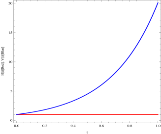
This result can be interpreted as an universe in an accelerated expansion q=βˆ’1π‘ž1q=-1, with a constant mean Hubble parameter and a volume involving with the cosmic time t𝑑t, as shown in the Figure 111. Due to the fact that H​(t)=H0𝐻𝑑subscript𝐻0H(t)=H_{0}, on has an universe of type de Sitter, where the effective density in (38) is constant, mimicking the cosmological constant.

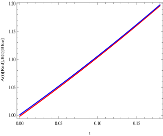
The scale factors in the directions xπ‘₯x and y𝑦y (also z𝑧z) are increasing, as represented in the Figure 222. At the beginning, the universe increases more rapidly in the direction y𝑦y, and later being equal to the others (isotropization).
Refer to caption
Figure 1: The graphs illustrating the evolution of the average Hubble parameter H​(t)𝐻𝑑H(t) and the volume V​(t)𝑉𝑑V(t) of the universe. The functions are plotted for c1=1subscript𝑐11c_{1}=1 and H0=1subscript𝐻01H_{0}=1.
Refer to caption
Figure 2: The graphs illustrating the evolution of the scale factors A​(t)𝐴𝑑A(t) and B​(t)𝐡𝑑B(t). The functions are plotted for c1=1subscript𝑐11c_{1}=1,   H0=1subscript𝐻01H_{0}=1,   T0=1subscript𝑇01T_{0}=1,   T2=1subscript𝑇21T_{2}=1,   λ=10βˆ’3πœ†superscript103\lambda=10^{-3}  and ΞΊ=0.9996711436381983πœ…0.9996711436381983\;\;\kappa=0.9996711436381983.

This is an isotropization model because the functions Ξ΄1​(t)subscript𝛿1𝑑\delta_{1}(t), in (48), and Δ​(t)Δ𝑑\Delta(t), in (45), tend to zero as the cosmic time goes toward infinity (px=py=pz=p=ω​ρsubscript𝑝π‘₯subscript𝑝𝑦subscriptπ‘π‘§π‘πœ”πœŒp_{x}=p_{y}=p_{z}=p=\omega\rho and A​(t)=B​(t)𝐴𝑑𝐡𝑑A(t)=B(t)). They are the anisotropic contributions for this model. The functions θ​(t),σ​(t)πœƒπ‘‘πœŽπ‘‘\theta(t),\sigma(t) and Δ​(t)Δ𝑑\Delta(t) are described in the Figure 333. One can see in these expressions that the isotropization is obtained at the limit Ξ»β†’0β†’πœ†0\lambda\rightarrow 0. We clearly see that it is the parameter Ξ»πœ†\lambda which governs the isotropization of the universe in this case. If Ξ»πœ†\lambda goes to infinity in (45), one gets the maximal anisotropy, so that Ξ”M​a​x=2subscriptΞ”π‘€π‘Žπ‘₯2\Delta_{Max}=2. Hence, Δ≀2Ξ”2\Delta\leq 2 in our case.

Refer to caption Refer to caption
Refer to caption
Figure 3: The graphs illustrating the evolution of the scalar expansion θ​(t)πœƒπ‘‘\theta(t), the shear scalar σ​(t)πœŽπ‘‘\sigma(t) and the anisotropy parameter Δ​(t)Δ𝑑\Delta(t). The functions are plotted for c1=1subscript𝑐11c_{1}=1,   H0=1subscript𝐻01H_{0}=1,   λ=10βˆ’3πœ†superscript103\lambda=10^{-3} and    ΞΊ=0.9996711436381983πœ…0.9996711436381983\kappa=0.9996711436381983.

One can define a function which gives the anisotropic measure by

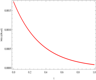
M​(t)=σ​(t)θ​(t)=3​H0​λ3​H0​λ+κ​e3​H0​t.π‘€π‘‘πœŽπ‘‘πœƒπ‘‘3subscript𝐻0πœ†3subscript𝐻0πœ†πœ…superscript𝑒3subscript𝐻0𝑑\displaystyle M(t)=\frac{\sigma(t)}{\theta(t)}=\frac{\sqrt{3}H_{0}\lambda}{3H_{0}\lambda+\kappa e^{3H_{0}t}}\,. (50)

The curve that shows the behaviour of the function M​(t)𝑀𝑑M(t) is described by the Figure 444, so that, the anisotropy fades away when the time goes to infinity.
Refer to caption
Figure 4: The graphs illustrating the evolution of the function M​(t)𝑀𝑑M(t). The function is plotted for c1=1subscript𝑐11c_{1}=1,   H0=1subscript𝐻01H_{0}=1,   T0=1subscript𝑇01T_{0}=1,    T2=1subscript𝑇21T_{2}=1\;,   λ=10βˆ’3πœ†superscript103\lambda=10^{-3} and    ΞΊ=0.9996711436381983πœ…0.9996711436381983\kappa=0.9996711436381983.

In the next section we will perform the reconstruction of the function f​(T)𝑓𝑇f(T) for a specific case of an anisotropic geometry. The analysis of the matter content of this present section also will be done in the next section for a whole comparison.

6 Reconstruction for LRS Bianchi type-I model in f​(T)𝑓𝑇f(T) Gravity

Here, we will consider that the anisotropic geometry is given by the same functions A​(t)𝐴𝑑A(t) and B​(t)𝐡𝑑B(t) in (42) and (43). Hence, we will get modifications in the matter content of the universe (the anisotropy of the fluid and the new contribution of the non-linear terms of T𝑇T). One has the same functions for the volume (35), the mean Hubble parameter (44), the scalar expansion and the shear in (49). Therefore, the model is clearly an isotropization model for the universe.

For finding a good model for this theory, we will use the so-called reconstruction method, because the algebraic function f​(T)𝑓𝑇f(T) is reconstructed according to the geometry and the matter content of the universe.

By introducing (42) and (43) into (23), we obtain the energy density of the fluid for the non-linear case

ρ2​(t)=116​π​[6​H02+f+12​H02​fTβˆ’54​H04​λ2​(1+2​fT)(e3​H0​t​κ+3​H0​λ)2].subscript𝜌2𝑑116πœ‹delimited-[]6superscriptsubscript𝐻02𝑓12superscriptsubscript𝐻02subscript𝑓𝑇54superscriptsubscript𝐻04superscriptπœ†212subscript𝑓𝑇superscriptsuperscript𝑒3subscript𝐻0π‘‘πœ…3subscript𝐻0πœ†2\displaystyle\rho_{2}(t)=\frac{1}{16\;\pi}\Big{[}6H_{0}^{2}+f+12H_{0}^{2}\;f_{T}-\frac{54H_{0}^{4}\;\lambda^{2}\;(1+2\;f_{T})}{(e^{3H_{0}t}\kappa+3H_{0}\lambda)^{2}}\Big{]}\,. (51)

After solving (27) and (29), we obtain the deviation-free part of anisotropic EoS parameter for the non-linear case:

Ο‰2(t)=116​π​ρ2​(t){βˆ’6H02+54​H04​λ2(e3​H0​t​κ+3​H0​λ)2βˆ’fβˆ’12H02[1βˆ’9​H02​λ2(e3​H0​t​κ+3​H0​λ)2]fT\displaystyle\omega_{2}(t)=\frac{1}{16\;\pi\;\rho_{2}(t)}\Big{\{}-6H_{0}^{2}+\frac{54H_{0}^{4}\;\lambda^{2}}{(e^{3H_{0}t}\kappa+3H_{0}\lambda)^{2}}-f-12H_{0}^{2}\left[1-\frac{9H_{0}^{2}\;\lambda^{2}}{(e^{3H_{0}t}\kappa+3H_{0}\lambda)^{2}}\right]\;f_{T}
+1296​H06​κ2​λ2​fT​T​e6​H0​t(e3​H0​t​κ+3​H0​λ)4},\displaystyle+\frac{1296H_{0}^{6}\;\kappa^{2}\;\lambda^{2}\;f_{T}T\;e^{6H_{0}t}}{(e^{3H_{0}t}\kappa+3H_{0}\lambda)^{4}}\Big{\}}\,, (52)

and the skewness parameter for the non-linear case as following

Ξ΄2​(t)subscript𝛿2𝑑\displaystyle\delta_{2}(t) =\displaystyle= 116​π​ρ2​(t)[βˆ’6H02βˆ’fβˆ’12H02fTβˆ’5832​H08​λ4​fT​T(e3​H0​t​κ+3​H0​λ)4βˆ’1944​H07​λ3​fT​T(e3​H0​t​κ+3​H0​λ)3\displaystyle\frac{1}{16\;\pi\;\rho_{2}(t)}\Big{[}-6H_{0}^{2}-f-12H_{0}^{2}\;f_{T}-\frac{5832H_{0}^{8}\;\lambda^{4}\;f_{TT}}{(e^{3H_{0}t}\kappa+3H_{0}\lambda)^{4}}-\frac{1944H_{0}^{7}\;\lambda^{3}\;f_{TT}}{(e^{3H_{0}t}\kappa+3H_{0}\lambda)^{3}} (54)
βˆ’54​H04​λ2​(2+fTβˆ’24​H02​fT​T)(e3​H0​t​κ+3​H0​λ)2βˆ’16πρ2(t)Ο‰2(t)].\displaystyle-\frac{54H_{0}^{4}\;\lambda^{2}\;(2+f_{T}-24H_{0}^{2}\;f_{TT})}{(e^{3H_{0}t}\kappa+3H_{0}\lambda)^{2}}-16\;\pi\;\rho_{2}(t)\omega_{2}(t)\Big{]}\,.

By replacing (42) and (43) into (17), we obtain the following relation:

t​(T)=1H0​log⁑[(3​λ​H0ΞΊ)1/3​(6​H06​H02+Tβˆ’1)1/3],𝑑𝑇1subscript𝐻0superscript3πœ†subscript𝐻0πœ…13superscript6subscript𝐻06superscriptsubscript𝐻02𝑇113\displaystyle t(T)=\frac{1}{H_{0}}\;\log\left[\left(\frac{3\lambda H_{0}}{\kappa}\right)^{1/3}\;\left(\frac{\sqrt{6}H_{0}}{\sqrt{6H_{0}^{2}+T}}-1\right)^{1/3}\right]\,, (55)

which leads to the equation of conservation for energy-momentum tensor

βˆ’52488​H010​λ5​[(6​H02+T)βˆ’6​H0​(6​H02+T)]​[f′​(T)βˆ’f′′​(T)](6​H02+T)2=0,52488superscriptsubscript𝐻010superscriptπœ†5delimited-[]6superscriptsubscript𝐻02𝑇6subscript𝐻06superscriptsubscript𝐻02𝑇delimited-[]superscript𝑓′𝑇superscript𝑓′′𝑇superscript6superscriptsubscript𝐻02𝑇20\displaystyle-\frac{52488H_{0}^{10}\;\lambda^{5}\;[(6H_{0}^{2}+T)-\sqrt{6}H_{0}\sqrt{(6H_{0}^{2}+T)}][f^{\prime}(T)-f^{\prime\prime}(T)]}{\;(6H_{0}^{2}+T)^{2}}=0\,, (56)

where the solution is given by:

f​(T)=T0+T1​eT,𝑓𝑇subscript𝑇0subscript𝑇1superscript𝑒𝑇\displaystyle f(T)=T_{0}+T_{1}\;e^{T}\,, (57)

where T0subscript𝑇0T_{0} and T1subscript𝑇1T_{1} are integration constants. The equations (51) and (52) become

ρ2​(t)subscript𝜌2𝑑\displaystyle\rho_{2}(t) =\displaystyle= 116​π[T0+T1exp[βˆ’6​H02​κ​e6​H0​t​(e3​H0​t​κ+6​H0​λ)(e3​H0​t​κ+3​H0​λ)2]\displaystyle\frac{1}{16\pi}\Big{[}T_{0}+T_{1}\;\exp\left[-\frac{6H_{0}^{2}\;\kappa e^{6H_{0}t}\;(e^{3H_{0}t}\kappa+6H_{0}\lambda)}{(e^{3H_{0}t}\kappa+3H_{0}\lambda)^{2}}\right] (58)
+H02(6+12T1exp[βˆ’6​H02​κ​e6​H0​t​(e3​H0​t​κ+6​H0​λ)(e3​H0​t​κ+3​H0​λ)2]\displaystyle+H_{0}^{2}\Big{(}6+12T_{1}\exp\left[-\frac{6H_{0}^{2}\;\kappa e^{6H_{0}t}\;(e^{3H_{0}t}\kappa+6H_{0}\lambda)}{(e^{3H_{0}t}\kappa+3H_{0}\lambda)^{2}}\right]
+54​H04​λ2​(βˆ’1βˆ’2​T1​exp⁑[βˆ’6​H02​κ​e6​H0​t​(e3​H0​t​κ+6​H0​λ)(e3​H0​t​κ+3​H0​λ)2])(e3​H0​t​κ+3​H0​λ)2)],\displaystyle+\frac{54H_{0}^{4}\lambda^{2}\left(-1-2T_{1}\exp\left[-\frac{6H_{0}^{2}\;\kappa e^{6H_{0}t}\;(e^{3H_{0}t}\kappa+6H_{0}\lambda)}{(e^{3H_{0}t}\kappa+3H_{0}\lambda)^{2}}\right]\right)}{(e^{3H_{0}t}\kappa+3H_{0}\lambda)^{2}}\Big{)}\Big{]},
Ο‰2​(t)=βˆ’XΞ±,subscriptπœ”2𝑑𝑋𝛼\displaystyle\omega_{2}(t)=-\frac{X}{\alpha}\,, (59)

where

X=[6H02+T0+T1exp[βˆ’6​H02​κ​e6​H0​t​(e3​H0​t​κ+6​H0​λ)(e3​H0​t​κ+3​H0​λ)2]βˆ’\displaystyle X=\Big{[}6H_{0}^{2}+T_{0}+T_{1}\exp\left[-\frac{6H_{0}^{2}\;\kappa e^{6H_{0}t}\;(e^{3H_{0}t}\kappa+6H_{0}\lambda)}{(e^{3H_{0}t}\kappa+3H_{0}\lambda)^{2}}\right]- (60)
1296​T1​H06​κ2​λ2​exp⁑[βˆ’6​H0​(e6​H0​t​(H0βˆ’t)​κ2+6​H0​κ​λ​e3​H0​t​(H0βˆ’t)βˆ’9​H02​t​λ2)(e3​H0​t​κ+3​H0​λ)2](e3​H0​t​κ+3​H0​λ)4βˆ’54​H04​λ2(e3​H0​t​κ+3​H0​λ)2+1296subscript𝑇1superscriptsubscript𝐻06superscriptπœ…2superscriptπœ†26subscript𝐻0superscript𝑒6subscript𝐻0𝑑subscript𝐻0𝑑superscriptπœ…26subscript𝐻0πœ…πœ†superscript𝑒3subscript𝐻0𝑑subscript𝐻0𝑑9superscriptsubscript𝐻02𝑑superscriptπœ†2superscriptsuperscript𝑒3subscript𝐻0π‘‘πœ…3subscript𝐻0πœ†2superscriptsuperscript𝑒3subscript𝐻0π‘‘πœ…3subscript𝐻0πœ†4limit-from54superscriptsubscript𝐻04superscriptπœ†2superscriptsuperscript𝑒3subscript𝐻0π‘‘πœ…3subscript𝐻0πœ†2\displaystyle\frac{1296T_{1}H_{0}^{6}\kappa^{2}\lambda^{2}\exp[-\frac{6H_{0}\Big{(}e^{6H_{0}t}(H_{0}-t)\kappa^{2}+6H_{0}\kappa\lambda e^{3H_{0}t}(H_{0}-t)-9H_{0}^{2}t\lambda^{2}\Big{)}}{(e^{3H_{0}t}\kappa+3H_{0}\lambda)^{2}}]}{(e^{3H_{0}t}\kappa+3H_{0}\lambda)^{4}}-\frac{54H_{0}^{4}\lambda^{2}}{(e^{3H_{0}t}\kappa+3H_{0}\lambda)^{2}}+ (61)
12H02ΞΊT1(e3​H0​tΞΊ+6H0Ξ»)exp[βˆ’6​H0​(e6​H0​t​(H0βˆ’t)​κ2+6​H0​κ​λ​e3​H0​t​(H0βˆ’t)βˆ’9​H02​t​λ2)(e3​H0​t​κ+3​H0​λ)2]],\displaystyle 12H_{0}^{2}\;\kappa\;T_{1}\;(e^{3H_{0}t}\kappa+6H_{0}\;\lambda)\exp[-\frac{6H_{0}\Big{(}e^{6H_{0}t}(H_{0}-t)\kappa^{2}+6H_{0}\kappa\lambda e^{3H_{0}t}(H_{0}-t)-9H_{0}^{2}t\lambda^{2}\Big{)}}{(e^{3H_{0}t}\kappa+3H_{0}\lambda)^{2}}]\Big{]}, (62)
Ξ±=T0+T1​exp⁑[βˆ’6​H02​κ​e6​H0​t​(e3​H0​t​κ+6​H0​λ)(e3​H0​t​κ+3​H0​λ)2]𝛼subscript𝑇0subscript𝑇16superscriptsubscript𝐻02πœ…superscript𝑒6subscript𝐻0𝑑superscript𝑒3subscript𝐻0π‘‘πœ…6subscript𝐻0πœ†superscriptsuperscript𝑒3subscript𝐻0π‘‘πœ…3subscript𝐻0πœ†2\displaystyle\alpha=T_{0}+T_{1}\exp\left[-\frac{6H_{0}^{2}\;\kappa e^{6H_{0}t}\;(e^{3H_{0}t}\kappa+6H_{0}\lambda)}{(e^{3H_{0}t}\kappa+3H_{0}\lambda)^{2}}\right] (63)
+H02(6+12T1exp[βˆ’6​H02​κ​e6​H0​t​(e3​H0​t​κ+6​H0​λ)(e3​H0​t​κ+3​H0​λ)2]\displaystyle+H_{0}^{2}\Big{(}6+12T_{1}\exp\left[-\frac{6H_{0}^{2}\;\kappa e^{6H_{0}t}\;(e^{3H_{0}t}\kappa+6H_{0}\lambda)}{(e^{3H_{0}t}\kappa+3H_{0}\lambda)^{2}}\right] (64)
+54​H04​λ2(e3​H0​t​κ+3​H0​λ)2​(βˆ’1βˆ’2​T1​exp⁑[βˆ’6​H02​κ​e6​H0​t​(e3​H0​t​κ+6​H0​λ)(e3​H0​t​κ+3​H0​λ)2]).54superscriptsubscript𝐻04superscriptπœ†2superscriptsuperscript𝑒3subscript𝐻0π‘‘πœ…3subscript𝐻0πœ†212subscript𝑇16superscriptsubscript𝐻02πœ…superscript𝑒6subscript𝐻0𝑑superscript𝑒3subscript𝐻0π‘‘πœ…6subscript𝐻0πœ†superscriptsuperscript𝑒3subscript𝐻0π‘‘πœ…3subscript𝐻0πœ†2\displaystyle+\frac{54H_{0}^{4}\lambda^{2}}{(e^{3H_{0}t}\kappa+3H_{0}\lambda)^{2}}\Big{(}-1-2T_{1}\exp\left[-\frac{6H_{0}^{2}\;\kappa e^{6H_{0}t}\;(e^{3H_{0}t}\kappa+6H_{0}\lambda)}{(e^{3H_{0}t}\kappa+3H_{0}\lambda)^{2}}\right]\Big{)}. (65)

The expression for the skewness parameter (54) is given by

Ξ΄2​(t)=βˆ’ZQ,subscript𝛿2𝑑𝑍𝑄\displaystyle\delta_{2}(t)=-\frac{Z}{Q}, (66)

where

Z=162H04Ξ»2(ΞΊ2exp[6​H0​(ΞΊ2​(H0+t)​e6​H0​t+6​H0​(H0+t)​e3​H0​t​λ​κ+9​t​H02​λ2)(e3​H0​t​κ+3​H0​λ)2]\displaystyle Z=162H_{0}^{4}\lambda^{2}\;\Big{(}\kappa^{2}\;\exp\left[\frac{6H_{0}(\kappa^{2}(H_{0}+t)e^{6H_{0}t}\;+6H_{0}\;(H_{0}+t)e^{3H_{0}t}\lambda\kappa+9\;tH_{0}^{2}\;\lambda^{2})}{(e^{3H_{0}t}\;\kappa+3H_{0}\lambda)^{2}}\right] (67)
+T1​κ2​e6​H0​t+6​H0​κ​λ​exp⁑[3​H0​(ΞΊ2​(2​H0+t)​e6​H0​t+6​H0​(2​H0+t)​e3​H0​t​λ​κ+9​t​H02​λ2)(e3​H0​t​κ+3​H0​λ)2]subscript𝑇1superscriptπœ…2superscript𝑒6subscript𝐻0𝑑6subscript𝐻0πœ…πœ†3subscript𝐻0superscriptπœ…22subscript𝐻0𝑑superscript𝑒6subscript𝐻0𝑑6subscript𝐻02subscript𝐻0𝑑superscript𝑒3subscript𝐻0π‘‘πœ†πœ…9𝑑superscriptsubscript𝐻02superscriptπœ†2superscriptsuperscript𝑒3subscript𝐻0π‘‘πœ…3subscript𝐻0πœ†2\displaystyle+T_{1}\kappa^{2}e^{6H_{0}t}+6H_{0}\;\kappa\;\lambda\;\exp\left[\frac{3H_{0}(\kappa^{2}(2H_{0}+t)e^{6H_{0}t}\;+6H_{0}\;(2H_{0}+t)e^{3H_{0}t}\lambda\kappa+9\;tH_{0}^{2}\;\lambda^{2})}{(e^{3H_{0}t}\;\kappa+3H_{0}\lambda)^{2}}\right] (68)
βˆ’6H0ΞΊΞ»T1e3​H0​t(6H02βˆ’1)+9H02Ξ»2exp[βˆ’6​H02​κ​e6​H0​t​(e3​H0​t​κ+6​H0​λ)(e3​H0​t​κ+3​H0​λ)2]+9H02T1Ξ»2),\displaystyle-6H_{0}\kappa\lambda T_{1}e^{3H_{0}t}(6H_{0}^{2}-1)+9H_{0}^{2}\lambda^{2}\exp\left[-\frac{6H_{0}^{2}\;\kappa e^{6H_{0}t}\;(e^{3H_{0}t}\kappa+6H_{0}\lambda)}{(e^{3H_{0}t}\kappa+3H_{0}\lambda)^{2}}\right]+9H_{0}^{2}T_{1}\lambda^{2}\Big{)}, (69)

and

Q=(e3​H0​tΞΊ+3H0Ξ»)2(ΞΊ2(6H02+T0)exp[6​H0​(ΞΊ2​(H0+t)​e6​H0​t+6​H0​(H0+t)​e3​H0​t​λ​κ+9​t​H02​λ2)(e3​H0​t​κ+3​H0​λ)2]\displaystyle Q=(e^{3H_{0}t}\kappa+3H_{0}\lambda)^{2}\Big{(}\kappa^{2}(6H_{0}^{2}+T_{0})\exp\left[\frac{6H_{0}(\kappa^{2}(H_{0}+t)e^{6H_{0}t}+6H_{0}(H_{0}+t)e^{3H_{0}t}\lambda\kappa+9tH_{0}^{2}\lambda^{2})}{(e^{3H_{0}t}\kappa+3H_{0}\lambda)^{2}}\right] (70)
+T1​κ2​e6​H0​t​(1+12​H02)+6​H0​κ​λ​(6​H02+T0)​exp⁑[3​H0​(ΞΊ2​(2​H0+t)​e6​H0​t+6​H0​(2​H0+t)​e3​H0​t​λ​κ+9​t​H02​λ2)(e3​H0​t​κ+3​H0​λ)2]subscript𝑇1superscriptπœ…2superscript𝑒6subscript𝐻0𝑑112superscriptsubscript𝐻026subscript𝐻0πœ…πœ†6superscriptsubscript𝐻02subscript𝑇03subscript𝐻0superscriptπœ…22subscript𝐻0𝑑superscript𝑒6subscript𝐻0𝑑6subscript𝐻02subscript𝐻0𝑑superscript𝑒3subscript𝐻0π‘‘πœ†πœ…9𝑑superscriptsubscript𝐻02superscriptπœ†2superscriptsuperscript𝑒3subscript𝐻0π‘‘πœ…3subscript𝐻0πœ†2\displaystyle+T_{1}\kappa^{2}e^{6H_{0}t}(1+12H_{0}^{2})+6H_{0}\kappa\lambda(6H_{0}^{2}+T_{0})\exp\left[\frac{3H_{0}(\kappa^{2}(2H_{0}+t)e^{6H_{0}t}+6H_{0}(2H_{0}+t)e^{3H_{0}t}\lambda\kappa+9tH_{0}^{2}\lambda^{2})}{(e^{3H_{0}t}\kappa+3H_{0}\lambda)^{2}}\right] (71)
+6H0ΞΊΞ»T1e3​H0​t(1+12H02)+9H02Ξ»2T0exp[6​H02​κ​e3​H0​t​(e3​H0​t​κ+6​H0​λ)(e3​H0​t​κ+3​H0​λ)2]+9H02T1Ξ»2).\displaystyle+6H_{0}\kappa\lambda T_{1}e^{3H_{0}t}(1+12H_{0}^{2})+9H_{0}^{2}\lambda^{2}T_{0}\exp\left[\frac{6H_{0}^{2}\kappa e^{3H_{0}t}(e^{3H_{0}t}\kappa+6H_{0}\lambda)}{(e^{3H_{0}t}\kappa+3H_{0}\lambda)^{2}}\right]+9H_{0}^{2}T_{1}\lambda^{2}\Big{)}. (72)

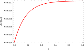
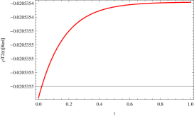
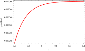
With the expressions of the energy densities (46) and (58), one represents this function in the Figure 555. Now, one can interpret the densities contributions. The density ρ1​(t)subscript𝜌1𝑑\rho_{1}(t) contributes lower than the energy density ρ2​(t)subscript𝜌2𝑑\rho_{2}(t), for the anisotropic expansion of the universe. Indeed, one calculates the diverse contributions of the effective energy densities in (38).
Refer to caption Refer to caption
Figure 5: The graphs illustrating the evolution of the energy density for the linear and non-linear cases (ρ1​(t)subscript𝜌1𝑑\rho_{1}(t) and ρ2​(t)subscript𝜌2𝑑\rho_{2}(t)). The functions are plotted for c1=1subscript𝑐11c_{1}=1,   H0=1subscript𝐻01H_{0}=1    T0=subscript𝑇0absentT_{0}=1    T2=1subscript𝑇21T_{2}=1,   λ=10βˆ’3πœ†superscript103\lambda=10^{-3}\;\; and ΞΊ=0.9996711436381983πœ…0.9996711436381983\kappa=0.9996711436381983.

With (44), (45), (57), (39) and (40), we have the density due to the torsion scalar terms and the density due to the anisotropy.

ρT​(2)​(t)=βˆ’116​π​exp⁑[βˆ’6​H02​κ​e3​H0​t​(κ​e3​H0​t+6​H0​λ)(κ​e3​H0​t+3​H0​λ)2],subscriptπœŒπ‘‡2𝑑116πœ‹6superscriptsubscript𝐻02πœ…superscript𝑒3subscript𝐻0π‘‘πœ…superscript𝑒3subscript𝐻0𝑑6subscript𝐻0πœ†superscriptπœ…superscript𝑒3subscript𝐻0𝑑3subscript𝐻0πœ†2\displaystyle\rho_{T(2)}(t)=-\frac{1}{16\pi}\exp\left[-\frac{6H_{0}^{2}\kappa e^{3H_{0}t}(\kappa e^{3H_{0}t}+6H_{0}\lambda)}{(\kappa e^{3H_{0}t}+3H_{0}\lambda)^{2}}\right], (73)
ρA​(2)​(t)=27​H04​λ28​π​(1+2​T1​exp⁑[βˆ’6​H02​κ​e3​H0​t​(κ​e3​H0​t+6​H0​λ)(κ​e3​H0​t+3​H0​λ)2])(κ​e3​H0​t+3​H0​λ)2.subscript𝜌𝐴2𝑑27superscriptsubscript𝐻04superscriptπœ†28πœ‹12subscript𝑇16superscriptsubscript𝐻02πœ…superscript𝑒3subscript𝐻0π‘‘πœ…superscript𝑒3subscript𝐻0𝑑6subscript𝐻0πœ†superscriptπœ…superscript𝑒3subscript𝐻0𝑑3subscript𝐻0πœ†2superscriptπœ…superscript𝑒3subscript𝐻0𝑑3subscript𝐻0πœ†2\displaystyle\rho_{A(2)}(t)=\frac{27H_{0}^{4}\lambda^{2}}{8\pi}\frac{\left(1+2T_{1}\exp[-\frac{6H_{0}^{2}\kappa e^{3H_{0}t}(\kappa e^{3H_{0}t}+6H_{0}\lambda)}{(\kappa e^{3H_{0}t}+3H_{0}\lambda)^{2}}]\right)}{(\kappa e^{3H_{0}t}+3H_{0}\lambda)^{2}}. (74)

The densities of the linear case are given by

ρT​(1)​(t)=0,subscriptπœŒπ‘‡1𝑑0\displaystyle\rho_{T(1)}(t)=0, (75)
ρA​(1)​(t)=27​H04​λ28​π​(κ​e3​H0​t+3​H0​λ)2.subscript𝜌𝐴1𝑑27superscriptsubscript𝐻04superscriptπœ†28πœ‹superscriptπœ…superscript𝑒3subscript𝐻0𝑑3subscript𝐻0πœ†2\displaystyle\rho_{A(1)}(t)=\frac{27H_{0}^{4}\lambda^{2}}{8\pi(\kappa e^{3H_{0}t}+3H_{0}\lambda)^{2}}. (76)

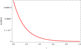
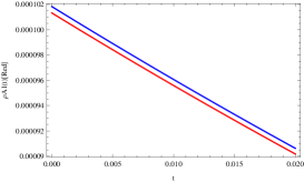
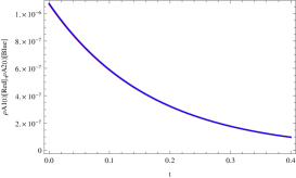
We represent the curves of the energy densities ρA​(1)​(t)subscript𝜌𝐴1𝑑\rho_{A(1)}(t) and ρA​(2)​(t)subscript𝜌𝐴2𝑑\rho_{A(2)}(t) at the left hand side in the Figures 666. We recall that at the left hand side there are two overlapping curves despite of seeming have one. In order to clearly show that there are effectively two different curves, within the same parameters and plotting in the range t∈(0,0.02)𝑑00.02t\in(0,0.02), the curve at the right hand side, it appears clearly that the two curves are distinct. One sees directly that the most important contribution is that of the model 222, i.e, the non-linear in T𝑇T. This is due to the negative contribution of the energy density ρT​(2)subscriptπœŒπ‘‡2\rho_{T(2)}, which is different from zero for the non-linear case (see Figure 777). So, the universe is more anisotropic at the beginning if the term of higher order on the torsion scalar are not considered. This is the main and interesting result obtained here, which is closest to the observational data.

Moreover, the energy densities combine, giving rise to a constant effective energy density, for getting a universe of type de Sitter. The two models do not interact.
Refer to caption Refer to caption
Figure 6: The graphs at the left hand side illustrates the evolution of the energy densities in (74) and (76), for the linear and non-linear cases in the inflationary phase, showing the decaying of the curves toward zero; while, the one at the right hand side exhibits the different between the curves. The functions are plotted for c1=1subscript𝑐11c_{1}=1,   H0=1subscript𝐻01H_{0}=1,    T0=1subscript𝑇01T_{0}=1,    T2=1subscript𝑇21T_{2}=1,   λ=10βˆ’3πœ†superscript103\lambda=10^{-3} and ΞΊ=0.9996711436381983πœ…0.9996711436381983\kappa=0.9996711436381983.
Refer to caption Refer to caption
Figure 7: The graphs illustrating the evolution of the energy densities in (73) and (75), for the linear and non-linear c1=1subscript𝑐11c_{1}=1,   H0=1subscript𝐻01H_{0}=1,    T0=1subscript𝑇01T_{0}=1,    T2=1subscript𝑇21T_{2}=1,   λ=10βˆ’3πœ†superscript103\lambda=10^{-3} and ΞΊ=0.9996711436381983πœ…0.9996711436381983\kappa=0.9996711436381983.

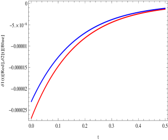
One can see very clearly this result through the figures 888 and 999. We see that the skewness parameter is negative in all two cases, however, lower absolute values for the second. This comes to show us that, due to the contribution of the non-linear terms of the function f​(T)𝑓𝑇f(T), the parameter Ξ΄2​(t)subscript𝛿2𝑑\delta_{2}(t) is more restricted, for small values within the real interval (βˆ’0.16,0.12)0.160.12(-0.16,0.12) [42] than the parameter Ξ΄1​(t)subscript𝛿1𝑑\delta_{1}(t) arising from the linear theory. So, we have the model with non-null f​(T)𝑓𝑇f(T), non-linear case, which is favoured by observational data, compared to the linear case.

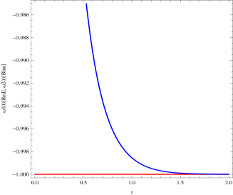
Also, in the same way, the parameter of EoS Ο‰1​(t)subscriptπœ”1𝑑\omega_{1}(t) is negative, but initially less than the case of Ο‰2​(t)subscriptπœ”2𝑑\omega_{2}(t).

Refer to caption
Figure 8: The graphs illustrating the evolution of the skewness parameter for the linear and non-linear cases (Ξ΄1​(t)subscript𝛿1𝑑\delta_{1}(t) and Ξ΄2​(t)subscript𝛿2𝑑\delta_{2}(t)). The functions are plotted for c1=1subscript𝑐11c_{1}=1,   H0=1subscript𝐻01H_{0}=1,    T0=1subscript𝑇01T_{0}=1,    T2=1subscript𝑇21T_{2}=1,   λ=10βˆ’3πœ†superscript103\lambda=10^{-3} and  κ=0.9996711436381983πœ…0.9996711436381983\kappa=0.9996711436381983.
Refer to caption
Figure 9: The graphs illustrating the evolution of the EoS parameters for the linear and non-linear cases (Ο‰1​(t)subscriptπœ”1𝑑\omega_{1}(t) and Ο‰2​(t)subscriptπœ”2𝑑\omega_{2}(t)). The functions are plotted for c1=1subscript𝑐11c_{1}=1,   H0=1subscript𝐻01H_{0}=1,   T0=1subscript𝑇01T_{0}=1,   T2=1subscript𝑇21T_{2}=1,   λ=1πœ†1\lambda=1   and   κ=1πœ…1\kappa=1.

In order to confirm our result, let us define, as in [51], the sum of the skewness parameters

Ξ”1​(t)=2​δ1​(t),Ξ”2​(t)=2​δ2​(t),formulae-sequencesubscriptΞ”1𝑑2subscript𝛿1𝑑subscriptΞ”2𝑑2subscript𝛿2𝑑\displaystyle\Delta_{1}(t)=2\delta_{1}(t)\,,\,\Delta_{2}(t)=2\delta_{2}(t)\,, (77)

which, from the dominant and strong-energy conditions [51], leads to the restriction

βˆ’3≀Δ1,2≀3.3subscriptΞ”123\displaystyle-3\leq\Delta_{1,2}\leq 3\,. (78)

We just have to observe the figure 888 ( multiplying by two), for seeing that both the models obey the restriction (78), i.e, Ξ”1,2≲10βˆ’5less-than-or-similar-tosubscriptΞ”12superscript105\Delta_{1,2}\lesssim 10^{-5}.

We can also observe the magnitude of σ​(t)πœŽπ‘‘\sigma(t), normalized by the average Hubble parameter, as in [52]. The restriction for this value is within the same range (βˆ’3,3)33(-3,3) [52]. By the figure 333, we see that R​(t)=3​σ​(t)/H​(t)≲10βˆ’2𝑅𝑑3πœŽπ‘‘π»π‘‘less-than-or-similar-tosuperscript102R(t)=\sqrt{3}\sigma(t)/H(t)\lesssim 10^{-2}, which confirms the validity of the two models.

We conclude defining the eccentricity as

ey2=[A​(t)B​(t)]2βˆ’1,superscriptsubscript𝑒𝑦2superscriptdelimited-[]𝐴𝑑𝐡𝑑21\displaystyle e_{y}^{2}=\left[\frac{A(t)}{B(t)}\right]^{2}-1\,, (79)

and the contribution of the quadrupole for the anisotropies of cosmic microwave background as being [52]

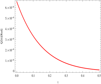
Q2=25​3​ey2.subscript𝑄2253subscriptsuperscript𝑒2𝑦\displaystyle Q_{2}=\frac{2}{5\sqrt{3}}e^{2}_{y}\,. (80)

Using (42), (43) and (80), one gets

Q2=25​3​[c12(ΞΊ/H0+3​λ​eβˆ’3​H0​t)2βˆ’1].subscript𝑄2253delimited-[]superscriptsubscript𝑐12superscriptπœ…subscript𝐻03πœ†superscript𝑒3subscript𝐻0𝑑21\displaystyle Q_{2}=\frac{2}{5\sqrt{3}}\left[\frac{c_{1}^{2}}{\left(\kappa/H_{0}+3\lambda e^{-3H_{0}t}\right)^{2}}-1\right]\,. (81)

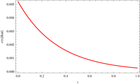
We present the graph of Q2​(t)subscript𝑄2𝑑Q_{2}(t) in the figure 101010. We see that both the models obey the restriction Q2​(t)≲10βˆ’6less-than-or-similar-tosubscript𝑄2𝑑superscript106Q_{2}(t)\lesssim 10^{-6}. Then, theses models are in agreement with the observational data, which restrain to Q2​(t)≲10βˆ’5less-than-or-similar-tosubscript𝑄2𝑑superscript105Q_{2}(t)\lesssim 10^{-5}.

Refer to caption
Figure 10: The graphs illustrating the evolution of the Q2​(t)subscript𝑄2𝑑Q_{2}(t) in (81). The functions are plotted for c1=1subscript𝑐11c_{1}=1,   H0=1subscript𝐻01H_{0}=1,    T0=1subscript𝑇01T_{0}=1,    T2=1subscript𝑇21T_{2}=1,   Ξ»=10βˆ’3πœ†superscript103\lambda=10^{-3} and ΞΊ=0.9996711436381983πœ…0.9996711436381983\kappa=0.9996711436381983.

7 Conclusion

In this work, locally rotationally symmetric Bianchi type-I model is considered in the framework of f​(T)𝑓𝑇f(T) theory of gravity where T𝑇T denotes the torsion scalar. With the corresponding metric, we wrote down the full equations of motion. We extensively performed the generalisation of anisotropic models with torsion and put a special emphasis on the isotropization process. Isotropization is an important aspect in cosmology and needs to receive particular attention, since in it evolution history, universe presents anisotropies at early time and comes becoming isotropic at present time according to the observational data. In this way, we first consider the linear case f​(T)=0𝑓𝑇0f(T)=0, where undertook the exponential expansion for scale factors. Then, we calculated the deviation-free part of the anisotropic EoS and the result reflects an accelerated expansion of the universe with q=βˆ’1π‘ž1q=-1, and a mean Hubble parameter and volume involving with time. Our analysis shows that at the beginning the universe presents unequal scalar factor in the directions xπ‘₯x and y𝑦y (anisotropy), and as the late-time is reached, they become equal (isotropy), reflecting the isotropization process.

Another interesting feature undertaken in this work is the reconstruction scheme of the algebraic function f​(T)𝑓𝑇f(T). We assumed the previous anisotropy expression of the scale factor and search for the action for which this anisotropy is realized. The result shows that the algebraic function is an exponential one. A whole comparison of these results with the linear case ones, as an important and interesting conclusion, is that the universe is more anisotropic at the beginning if the terms of higher order in torsion scalar are not considered. This means that the non-linear model should be favoured by observational data.

Acknowledgement: M. E. Rodrigues thanks a lot PPGF of the UFPA for the hospitality during the elaboration of this work and also CNPq for financial support. I. G. SALAKO thanks ICTP/IMSP for partial financial support.

References

  • [1] S. Perlmutter et al. [SNCP Collaboration], Astrophys. J. 517, 565 (1999); A. G. Riess et al. [SNST Collaboration], Astron. J.116, 1009 (1998).
  • [2] S. Nojiri and S. D. Odintsov, Phys. Rept. 505, 59 (2011); eConf C0602061, 06 (2006) [Int.J. Geom. Meth. Mod. Phys. 4, 115 (2007)] [arXiv:hep-th/0601213].
  • [3] T. P. Sotiriou and V. Faraoni, Rev. Mod. Phys. 82, 451 (2010).
  • [4] A. De Felice and S. Tsujikawa, Living Rev. Rel. 13, 3 (2010).
  • [5] T. Clifton, P. G. Ferreira, A. Padilla and C. Skordis, arXiv:1106.2476 [astro-ph.CO].
  • [6] K. Bamba, C.-Q. Geng, S. Nojiri, S. D. Odintsov, arXiv:0909.4397.
  • [7] M. J. S. Houndjo, M. E. Rodrigues, D. Momeni, R. Myrzakulov .arXiv:1301.4642 [gr-qc].
  • [8] M.E. Rodrigues, M.J.S. Houndjo, D. Momeni, R. Myrzakulov, arXiv:1212.4488.
  • [9] K. Bamba, S. D. Odintsov, L. Sebastiani, S. Zerbini, arXiv:0911.4390.
  • [10] S. Nojiri, S. D. Odintsov, A. Toporensky, P. Tretyakov, arXiv:0912.2488.
  • [11] G. Cognola, E. Elizade, S. Nojiri, S. D. Odintsov and S. Zerbini, Phys. Rev. D 73 084007 (2006) [arxiv:hep-th/0601008].
  • [12] E. Elizalde, R. Myrzakulov, V. V. Obukhov and D. SΓ‘ez-GΓ³mez, Class. Quant. Grav.27 (2010) 095007 [arXiv:1001.3636 [gr-qc]].
  • [13] R. Myrzakulov, D. SΓ‘ez-GΓ³mez and A. Tureanu, Gen. Rel. Grav. 43 (2011) 1671 [arXiv:1009.0902[gr-qc]].
  • [14] A. De Felice and T. Suyama, JCAP 0906, 034 (2009); Phys. Rev. D 80, 083523 (2009); Prog. Theor. Phys. 125, 603 (2011); A. De Felice, J. -M. Gerard and T. Suyama, Phys. Rev. D 82,063526 (2010).
  • [15] A. De Felice and S. Tsujikawa, Phys. Lett. B 675, 1 (2009) [arXiv:0810.5712 [hep-th]].
  • [16] A. De Felice, D. F. Mota and S. Tsujikawa, Phys. Rev. D 81, 023532 (2010) [arXiv:0911.1811 [gr-qc]].
  • [17] A. De Felice and T. Tanaka, Prog. Theor. Phys. 124, 503 (2010).
  • [18] S. Nojiri, S. D. Odintsov, Phys. Lett. B 631 1 (2005) [arxiv:hep-th/0508049]; Phys. Rev. D 68,123512 (2003) [hep-th/0307288].
  • [19] F. G. Alvarenga, M. J. S. Houndjo, A. V. Monwanou and Jean. B. Chabi-Orou,€ J. Mod. Phys.4, 130-139 (2013), arXiv: 1205.4678 [gr-qc].
  • [20] M. J. S. Houndjo, C. E. M. Batista, J. P. Campos and O. F. Piattella,€ Can. J. Phys. 91, 548-553 (2013), [arXiv:1203.6084 [gr-qc]].
  • [21] D. Momeni, M. Jamil and R. Myrzakulov, Euro. Phys. J. C 72, arXiv: 1107.5807[physics.gen-ph].
  • [22] M. J. S. Houndjo and O. F. Piattella€, Int. J. Mod. Phys. D. 21, 1250024 (2012). arXiv: 1111.4275 [gr.qc].
  • [23] M. J. S. Houndjo, Int. J. Mod. Phys. D. 21, 1250003 (2012). arXiv: 1107.3887 [astro-ph.CO].
  • [24] T. Harko, F. S. N. Lobo, S. Nojiri and S. D. Odintsov, Β€Βœf​(R,T)𝑓𝑅𝑇f(R,T) gravity,€ Phys. Rev. D 84 (2011) 024020. [arXiv:1104.2669 [gr-qc]].
  • [25] M. J. S. Houndjo, D. Momeni and R. Myrzakulov, Int. J. Mod. Phys. D 21 (2012) 1250093 [arXiv:1206.3938 [physics.gen-ph]].
  • [26] R. Ferraro and F. Fiorini, Phys. Rev. D 75, 084031 (2007). [arXiv:gr-qc/0610067]
  • [27] G. R. Bengochea, R. Ferraro and , Phys. Rev. D 79, 124019 (2009) [arXiv:0812.1205 [astro-ph]].
  • [28] N. Tamanini and C. G. Boehmer, Phys. Rev. D 86, 044009 (2012), arXiv:1204.4593 [gr-qc].
  • [29] M. H. Daouda, M. E. Rodrigues and M. J. S. Houndjo, Phys. Lett. B 715 (2012) 241 [arXiv:1202.1147 [gr-qc]]; Eur. Phys. J. C 72 (2012) 1893 [arXiv:1111.6575 [gr-qc]]; Eur. Phys. J. C 72 (2012) 1890 [arXiv:1109.0528 [physics.gen-ph]]; Eur. Phys. J. C 71 (2011) 1817 [arXiv:1108.2920 [astro-ph.CO]].
  • [30] M. E. Rodrigues, M. J. S. Houndjo, D. Saez-Gomez and F. Rahaman, Phys. Rev. D 86 (2012) 104059 [arXiv:1209.4859 [gr-qc]].
  • [31] M. Hamani Daouda, M. E. Rodrigues and M. J. S. Houndjo, Eur. Phys. J. C 72 (2012) 1893 [arXiv:1111.6575 [gr-qc]].
  • [32] M. Hamani Daouda, M. E. Rodrigues and M. J. S. Houndjo, Eur. Phys. J. C 72 (2012) 1890 [arXiv:1109.0528 [physics.gen-ph]].
  • [33] M. E. Rodrigues, M. J. S. Houndjo, D. Momeni and R. Myrzakulov, International Journal of Modern Physics D 22, 135004 (2013), arXiv:1302.4372 [physics.gen-ph].
  • [34] M. J. S. Houndjo, D. Momeni, R. Myrzakulov and M. E. Rodrigues,arXiv:1304.1147.
  • [35] M. Hamani Daouda, M. E. Rodrigues and M. J. S. Houndjo, Eur. Phys. J. C 71 (2011) 1817 [arXiv:1108.2920 [astro-ph.CO]].
  • [36] I. G. Salako, M. E. Rodrigues, A. V. Kpadonou, M. J. S. Houndjo, J. Tossa   [arXiv:1307.0730]
  • [37] M. J. S. Houndjo, D. Momeni and R. Myrzakulov, Int. J. Mod. Phys. D 21 (2012) 1250093 [arXiv:1206.3938 [physics.gen-ph]].
  • [38] M. E. Rodrigues, M. H. Daouda and M. J. S. Houndjo, arXiv:1205.0565 [gr-qc].
  • [39] M. R. Setare and M. J. S. Houndjo, Can. J. Phys. 91, 260-267; arXiv:1203.1315 [gr-qc].
  • [40] Carlos R. Fadragas, Genly Leon, Emmanuel N. Saridakis, arXiv:1308.1658 [gr-qc].
  • [41] Michele Fontanini, Mark Trodden, Eric J. West, Phys. Rev. D 80, 123515 (2009); arXiv:0905.3727 [astro-ph.CO].
  • [42] L. Campanelli, P. Cea, G.L. Fogli, A. Marrone, Phys. Rev. D 83, 103503 (2011). arXiv:1012.5596 [astro-ph.CO].
  • [43] Claudia Quercellini, Miguel Quartin and Luca Amendola, PRL 102: 151302 (2009) [arXiv:0809.3675 [astro-ph]].
  • [44] Claudia Quercellini, Luca Amendola, Amedeo Balbi, Paolo Cabella, Miguel Quartin, Physics Reports, 521, 95-134 (2012).
  • [45] L. Baojiu, T. P. Sotiriou, and J.D. Barrow, Phys. Rev. D 83, 064035 (2011); Phys.Rev.D 83:104030 (2011).
  • [46] M. Hamani Daouda, Manuel E. Rodrigues, M. J. S. Houndjo, Eur. Phys. J. C. 71 1817 (2011), arXiv:1108.2920v4 [astro-ph.CO]; Euro. Phys. J. C 72 1890 (2012), arXiv:1109.0528v4 [physics.gen-ph].
  • [47] M. Hamani Daouda, Manuel E. Rodrigues and M. J. S. Houndjo, arXiv:1205.0565v1 [gr-qc].
  • [48] Cemsinan Deliduman and Baris Yapiskan, arXiv:1103.2225 [gr-qc].
  • [49] C. B. Collins and S. W. Hawking, Astrophys. Journal, 180: 317-334 (1973).
  • [50] Cyril Pitrou, Thiago S. Pereira, Jean-Philippe Uzan, JCAP 0804:004 (2008) [arXiv:0801.3596 [astro-ph]].
  • [51] John D. Barrow, Phys.Rev. D 55: 7451-7460 (1997)[arXiv:gr-qc/9701038].
  • [52] Tomi Koivisto and David F. Mota, JCAP 0806: 018 (2008) [arXiv:0801.3676 [astro-ph]].