Peculiar velocity decomposition, redshift space distortion and velocity reconstruction in redshift surveys. II. Dark matter velocity statistics
Abstract
Massive spectroscopic redshift surveys open a promising window to accurately measure peculiar velocity at cosmological distances through redshift space distortion (RSD). In Paper I Zhang et al. (2013) of this series of work, we proposed decomposing peculiar velocity into three eigenmodes (, and ) in order to facilitate the RSD modeling and peculiar velocity reconstruction. In the current paper we measure the dark matter RSD-related statistics of the velocity eigenmodes through a set of N-body simulations. These statistics include the velocity power spectra, correlation functions, one-point probability distribution functions, cumulants, and the damping functions describing the Finger of God effect. We have carried out a number of tests to quantify possible numerical artifacts in these measurements and have confirmed that these numerical artifacts are under control. Our major findings are as follows: (1) The power spectrum measurement shows that these velocity components have distinctly different spatial distribution and redshift evolution, consistent with predictions in Paper I. In particular, we measure the window function . describes the impact of nonlinear evolution on the -density relation. We confirm that the approximation can induce a significant systematic error of in RSD cosmology. We demonstrate that can be accurately described by a simple fitting formula with one or two free parameters. (2) The correlation function measurement shows that the correlation length is , , and Mpc for , , and respectively. These correlation lengths determine where we can treat the velocity fields as spatially uncorrelated. Hence, they are important properties in RSD modeling. (3) The velocity probability distribution functions and cumulants quantify non-Gaussianities of the velocity fields. We confirm speculation in Paper I that is largely Gaussian, but with non-negligible non-Gaussianity. We confirm that is significantly non-Gaussian. We also measure the damping functions. Despite the observed non-Gaussianities, the damping functions and hence the Finger of God effect are all well approximated as Gaussian ones at scales of interest.
pacs:
98.80.-k; 98.80.Es; 98.80.Bp; 95.36.+xI Introduction
Redshift space distortion (RSD) is emerging as a powerful probe of dark energy and gravity at cosmological scales Jackson (1972); Sargent and Turner (1977); Peebles (1980); Kaiser (1987); Peacock and Dodds (1994); Ballinger et al. (1996); Peacock et al. (2001); Tegmark et al. (2002, 2004); Amendola et al. (2005); Linder (2005); Yamamoto et al. (2005); Zhang et al. (2007); Guzzo et al. (2008); Wang (2008); Percival and White (2009); Song and Percival (2009); White et al. (2009); Song (2011); Wang et al. (2010); Blake et al. (2011); Samushia et al. (2012); Blake et al. (2012); Reid et al. (2012a); Tojeiro et al. (2012a); Jain and Zhang (2008); Linder (2008); Reyes et al. (2010); Cai and Bernstein (2012); Gaztañaga et al. (2012); Jennings et al. (2012); Li et al. (2013); Schlegel et al. (2011); Laureijs et al. (2011). However, RSD modeling is highly complicated (e.g., Scoccimarro (2004); Seljak and McDonald (2011); Okumura et al. (2012a, b); Bonoli and Pen (2009); Desjacques and Sheth (2010) and references therein), due to entangled nonlinearities in the velocity and density fields and in the real space-redshift space mapping.
RSD is induced by peculiar motion. Naturally the first step to understand RSD is to understand the peculiar velocity . It turns out that different components of affect RSD in different ways. Motivated by it, we proposed a unique decomposition of into three eigenmodes (Paper I, Zhang et al. (2013)). The three components are not only uniquely defined mathematically, but also have unique physical meanings and have different impacts on RSD. We find that this decomposition indeed facilitates the RSD modeling. It helps us in arriving at a new RSD formula. It also helps us in proposing new approaches to reconstruct three-dimensional peculiar velocity at cosmological distances through spectroscopic redshift surveys.
Paper I outlined the basic methodology, but left most quantitative analysis for future studies. The present paper (Paper II) is the second paper of the series, focusing on the RSD-related dark matter velocity statistics. Future works will extend to the halo velocity statistics and eventually to the galaxy velocity statistics. We will evaluate the accuracy of the proposed RSD formula for dark matter and galaxies. We will also investigate the proposed velocity reconstruction techniques.
This paper is organized as follows. §II briefly describes the three velocity components. §III describes the simulations and the velocity assignment method used for the analysis. Numerical artifacts are quantified through several tests detailed in the Appendix and are proven to be under control. §IV shows the results of relevant velocity statistics. We summarize and discuss in §V.
II Theory basics
Paper I proposed decomposing the velocity into three eigenmodes (, , and ). This decomposition allows us to conveniently derive the leading-order RSD corrections in the redshift space power spectrum. For the dark matter redshift space power spectrum,
Here, . The FOG effect is described by the damping function
| (2) |
We predict in paper I that only contributes to the Finger of God (FOG) effect through . causes both an enhancement () and a damping (). All other terms in Eq. (II) are contributed by . For more details, refer to Paper I. Here we just summarize the basic results of the three velocity components, with terms in Eq. (II) explained.
is irrotational () and is completely correlated with the underlying density field . The relation in Fourier space is
| (3) | |||||
Here, and . is the power spectrum between the field and the field , defined as . We often use the notation , which enters into the ensemble average . If and are vector fields, .
In the limit , for the matter field 111For the galaxy field, in the limit . Refer to paper I for detailed discussions. . Here, is the linear density growth factor. Clearly contains most information of RSD cosmology. Nonlinear evolution causes at small scales to deviate from the linear theory prediction. Such deviation is described by the dimensionless
| (4) |
This definition is slightly different from that in Paper I. But for CDM, in which is scale independent, the two definitions are identical. But in modified gravity models or in models with dark energy fluctuations, is scale dependent. defined in this way, hence, isolates the impact of nonlinear evolution from the scale dependence in linear evolution. We expect in general, even for modified gravity models and models with dark energy fluctuations.
We find that can deviate from unity by at Mpc. It modifies the Kaiser formula (for dark matter RSD) from to . So if the is not taken into account, can be biased low by , as predicted by perturbation theory. A systematic error of such amplitude is severe for stage IV dark energy surveys like BigBOSS/MS-DESI Big , CHIME CHI , Euclid Euc and SKA SKA . In the present paper we will quantify more robustly, through N-body simulations.
causes both large-scale enhancement and small-scale damping in the redshift space clustering. Besides the correction, nonlinearities in induce complicated high order corrections ( and ) to the Kaiser effect in RSD modeling (Paper I). These high-order corrections involve both the velocity and density fields, so quantifying them is beyond the scope of this paper and will be left for future investigation through N-body simulations. In principle, nonlinearities in also complicate the FOG effect.
is also irrotational (). But to the opposite of , it is uncorrelated with the underlying density field (). This velocity component arises from nonlinear evolution. It is the cause of density-velocity stochasticity,
| (5) | |||||
causes both large-scale enhancement and small-scale damping in the redshift space clustering. But notice that the leading-order large-scale enhancement has a angular dependence [Eq. (II)]. It hence differs significantly from the Kaiser effect.
is the curl (rotational) component, satisfying . grows only after orbit crossing occurs. We expect its power to concentrate at small scales. We also expect that, to a good approximation, it only damps the redshift space clustering and only induces the FOG effect.
The present paper aims to quantify the RSD-related statistics of the three velocity components, through simulations. These statistics include
-
•
the power spectra ,
-
•
and in particular the - relation,
-
•
the correlation functions and ,
-
•
, the probability distribution functions (PDFs) of along the axis, and their derived properties such as cumulants and the FOG function .
Here, the subscript denotes the three velocity components.
III N-body simulation and velocity assignment method
Given the involved nonlinearities, N-body simulations are needed to robustly quantify the above velocity statistics. Furthermore, comprehensive tests must be designed and performed to robustly quantify numerical artifacts associated with simulations themselves and numerical artifacts associated with the velocity assignment method.
III.1 N-body simulations
| Name | Mpc | |||
|---|---|---|---|---|
| J1200 | 1200 | 0.045 | ||
| J300 | 300 | 0.045 | ||
| G100 | 100 | 0.044 |
From the structure formation theory, we expect that dominates at linear/large scales while and become important at sufficiently nonlinear/small scales. Given the computation limitation, it would be difficult for a single simulation to robustly evaluate all three components. A natural remedy is to combine large box simulations with small box simulations. Large box simulations help us better understanding the velocity field at large scales , in particular . Small box simulations have high mass and force resolution, so they can probe and more robustly. Combining these results, we can then circumvent the computation limitation and accurately study the statistical properties of the three velocity components.
For this reason, we combine three high-resolution (particle number ) dark matter simulations with box size , , and . For brevity, we will refer to them as J1200, J300, and G100, respectively. The simulations utilize standard CDM cosmology with flat space and Gaussian initial conditions. Simulation specifications are listed in Table 1. The adopted cosmological parameters are identical, expect a slight difference in the baryon density . For the purpose of our work, we can safely neglect this difference. J1200 and J300 are run with a particle-particle-particle-mesh () code (see Jing et al. (2007) for details). G100 is run with Gadget2 Springel et al. (2001); Springel (2005). For J1200 and G100, we analyze four redshift snapshots, respectively, which are of J1200 and of G100. Some output redshifts of J1200 differ from corresponding ones of G100 by . The linear velocity growth rate is , where and is the linear density growth factor. So these differences in result in 222This is a rough estimation based on the approximation and . Under these approximations, we have . in velocity. The major purpose of this paper is to identify the three velocity components and their basic statistics. For this purpose we can safely neglect these redshift differences in the current paper. For brevity we refer to the four snapshots as hereafter. Nevertheless, eventually we need to analyze simulations at identical redshifts. We also need to run many realizations to robustly quantify the velocity statistics. For J300, we only analyze its snapshot since it is mainly used to test our velocity assignment method in the Appendix (Fig. 12).
III.2 The velocity assignment method
It is tricky to properly estimate the volume-weighted velocity field from velocities of inhomogeneously distributed dark matter particles or galaxies (e.g. Bernardeau and van de Weygaert (1996) and references therein). In N-body simulations, we only have limited simulation particles and only have the velocity information at positions of these particles. However, the velocity where there is no particle is not necessarily small/negligible. In contrast, since the velocity is determined by the large-scale matter distribution, velocity in low-density regions/voids can be large and in general non-negligible. This sampling bias is difficult to correct from first principles, especially due to the awkward situation that the velocity and density fields are neither completely correlated nor completely uncorrelated.
We take a simple procedure to estimate the volume weighted velocity field in simulations. For a given grid point, we assign the velocity of its nearest dark matter particle/halo/galaxy to it. We call this method the nearest-particle (NP) method. The probability for a particle’s velocity to be assigned to a grid is inversely proportional to its ambient particle number density , , where denotes the volume it occupies. So the NP velocity assignment method indeed constructs a volume-weighted velocity field 333 J. Koda kindly showed us their ongoing work Koda et al. (2013), which also proposed the NP method. This work also quantified and corrected the alias effect of the NP method. .
We emphasize that this velocity assignment method is different to the widely used nearest-grid-point (NGP) method in constructing the density field. For NGP, each particle looks for its nearest grid point and assigns itself to this grid point. All particles are used in the assignment. But for NP, each grid point looks for its nearest particle and is assigned with the particle velocity. In dense regions, only a fraction of particles are used in the assignment. In underdense regions, some particles are used repeatedly and their velocities are assigned to more than one grid point. In this sense, it does not use all information of particles. A simple remedy is to shift the grids so another set of particles is used for the velocity assignment.
We also emphasize the difference between the NP method and the Voronoi tessellation (VT) method Bernardeau and van de Weygaert (1996). The first step of the VT method is to fill the space with polyhedral cells. Each polyhedron contains only one particle, and it covers all space points who consider this particle to be their nearest particle. The velocity within this polyhedron is assigned to be the velocity of that particle. The next step is to smooth the velocity field over a given window function to obtain the velocities on regular grids. We realize that the NP method is essentially the first step of the VT method. However, unlike the VT method, the NP method does not apply a smoothing. This is to avoid artificial suppression of small-scale random motions, which are real signals of significant impact on the FOG effect. This artificial suppression of small scale velocity components also exists in the widely adopted Delaunay tessellation (DT) method Bernardeau and van de Weygaert (1996); van de Weygaert and Schaap (2009); Pueblas and Scoccimarro (2009). This is the major reason that we do not adopt this method 444The Delaunay Tessellation (DT) velocity assignment utilizes a two-step scheme to get a volume-weighted velocity field: first it produces a Delaunay tessellation by linking the closest 4 particles to form a tetrahedron network. The velocity field inside one tetrahedron is determined through linearly interpolating the velocities at its 4 vertices. Then the velocity field is smoothed over a given window function to obtain the velocities on regular grids. The DT method has been proved to be accurate and reliable at linear and quasi-linear scales (e.g. Bernardeau and van de Weygaert (1996); Pueblas and Scoccimarro (2009); van de Weygaert and Schaap (2009)). However it breaks down at nonlinear regimes where shell-crossings and multi-stream flows occur van de Weygaert and Schaap (2009). In these regions, the linear interpolation tends to underestimate the velocity by averaging velocities with different directions. The smoothing procedure further smoothes out random (but real) motions at small scales. Since most contribution to and comes from nonlinear scales, the DT method could significantly underestimate and . .
The NP method is straightforward to implement. Furthermore, it is robust in a number of aspects, despite its simplicity: (1) In high-density regions, NP does not cause underestimation in the (one-dimensional) velocity dispersion , since it does not average over particle velocities. This is important for RSD study, otherwise, underestimation of will cause underestimation of FOG. (2) It robustly measures , which is of the most importance for RSD cosmology. For the NP velocity assignment, high-density regions are no problem because there are always particles within a grid size. In underdense regions, the typical distance from a given grid point to its nearest particle is , which can be large. But in such regions does not vary strongly, since its typical length of variation is roughly given by [Eq. (3)]. The requirement to robustly sample is then
This condition is not difficult to satisfy for typical simulation specifications today. For example, for our J1200 simulation, Mpc and the above condition is usually satisfied. Notice that and ( at ). An exception is the very underdense regions with . In these regions, our simulation undersamples the field. But these regions are very rare and we do not expect this undersampling to be severe for statistically evaluating the field. (3) The NP method does not use the velocity information of all particles. Nevertheless, the information encoded in unused particles can be captured by shifting the grids and resampling the velocity field, when necessary.
III.3 The velocity decomposition method
After sampling the velocity field on regular grids by the NP method, we proceed to decompose into the three eigenmodes. The velocity decomposition is conveniently operated in Fourier space. First we make the E/B decomposition,
| (7) | |||||
Then we decompose into and [ Eq. (3)] 555The sign of expression being plus or minus depends on the definition of Fourier transform. Our definition for Fourier transform is .,
| (8) | |||||
Here is the Hubble parameter at redshift , and the window function is calculated in advance by . The density field is sampled by the NGP method on the same regular grids as the velocity field. When calculating , we do not correct the shot noise term since it is negligible for our high particle number density simulation. Also we do not correct other numerical artifacts like smoothing and alias effects, which are subdominant to systematic errors induced by the velocity assignment method. Hence, numerical artifacts quantified by our designed tests (Appendix A) receive minor contribution from those in the density field.
III.4 Testing the NP method
In Appendix A we design and carry out several tests to verify the robustness of the NP method for our study.
First we compare the power spectra of the three velocity components between different box sizes, grid numbers, and particle numbers. Discrepancies there diagnose sampling bias. In particular, the NP method becomes exact in the limit . By constructing the velocity field using a fraction of particles and observing its dependence on the particle numbers, we can evaluate its accuracy. If the results converge, we then have confidence of vanishing sampling bias. Detailed comparison is given in Appendix A.
In brief, we find that NP method can construct and fields quite reliably. However, for large box simulations (e.g. J1200), the amplitude is significantly overestimated at all scales due to a shot-noise-like alias effect induced by sparse sampling Pueblas and Scoccimarro (2009). However, tests on small box simulation G100 show reasonable convergence of . So the G100 simulation provides reasonably accurate measure of . Hence, in combination of J1200 and G100, we have reliable measures of all three velocity components.
We also test the NP method against the fiducial velocity field of known statistics as input (§A.2). This test is particularly good at highlighting leakage between the three velocity components. We do find such leakages. We quantify their amplitudes as a function of scales and identify regions where these leakages are under control.
These tests show that, combining J1200 and G100, we can control numerical artifacts and reliably measure all three velocity components. Even better, the impacts of these numerical artifacts on RSD cosmology are further reduced for a number of reasons. First, the majority of cosmological information resides in relatively large scales and especially in . This component is accurately measured. Second, although accurate measurement of is more challenging, its impact on RSD is fully captured by its velocity dispersion (Sec. IV), which can be treated as a free parameter to be fitted against data. Even simpler, Sec. IV will show that setting is already sufficiently accurate for RSD modeling.
IV Statistics of
Understanding the statistical properties of the three velocity components facilitates the RSD modeling and velocity reconstruction (Paper I). For this purpose, we measure the one-point and two-point velocity statistics from simulations. (1) The velocity power spectra () go directly into the redshift space matter power spectrum. They also quantify the scale dependence and redshift evolution of these velocity components. They are useful to understand the physical origins of these velocity components. The window function is a derived quantity of these power spectra. (2) Velocity correlation functions and () quantify the velocity correlation length, . These correlation lengths are crucial in judging at which separation we can treat the velocities at two positions as independent. Basically, if the scale of interest , we can safely ignore the intrinsic clustering of the field. In this limit, we can treat as a random field in RSD modeling, whose impact is fully captured by a damping function . Otherwise, we have to take their intrinsic clustering into account, which contributes extra power to the redshift space clustering. (3) Finally, we will quantify the non-Gaussianities of the velocity fields, through the one-point PDF and the reduced cumulants . These non-Gaussianity measures are highly relevant for modeling , which describes the FOG effect.
IV.1 The velocity power spectrum
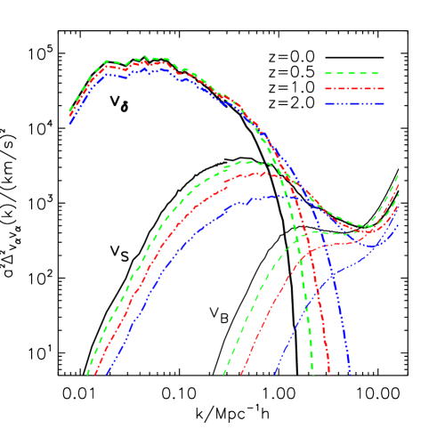
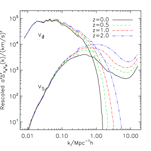
The velocity power spectra at are shown in Fig. 1. These results confirm our speculation in Paper I, based upon the structure formation theory. It shows that is the dominant component at linear and mildly nonlinear scales. Perturbation theory predicts that it evolves linearly at sufficiently large scales, with the linear velocity growth factor
| (9) |
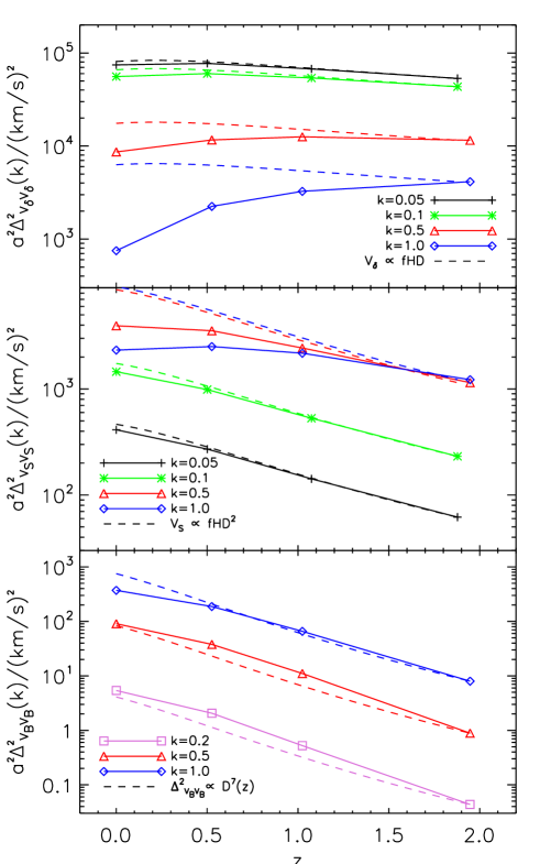
Figures. 2 and 3 verify this linear evolution at Mpc. However, linear perturbation theory quickly loses its predicting power at Mpc. Even at Mpc, impact of nonlinear evolution is visible.
Nonlinear evolution in the velocity and density fields drive to decrease from unity. is one of the most important properties to describe the velocity field, to model RSD, and to reconstruct velocity in spectroscopic surveys. Hence we devote the whole Sec. IV.2 to discuss it.
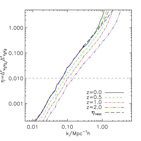
Nonlinear evolution also induces stochasticity in the velocity-density relation and causes the emergence of (Fig. 1). It eventually dominates over at Mpc and . To better show its impact, Fig. 4 plots the ratio . Stage IV dark energy projects such as BigBOSS/MS-DESI, CHIME, Euclid, and SKA can achieve level statistical precision for the velocity measurement through RSD. So once , the component becomes non-negligible in RSD modeling. reaches at Mpc and (Fig. 4). Even at high redshift , at Mpc. These results agree with calculation by high-order perturbation theory (Fig. 1, Paper I). It confirms our conclusion in Paper I that, in general is a non-negligible velocity component, even at scales which are often considered as linear. Its contribution to the redshift space matter power spectrum will be quantitatively studied in future works. Future work will also explore information encoded in . For example, it may be used to probe the environmental dependence of modified gravity theories (Paper I).
Perturbation theory is also useful to understand the redshift evolution of . From the continuity equation,
| (10) |
the leading-order contribution to comes from and . Here, is the sum over contributions of th order density component. To a good approximation, Bernardeau et al. (2002). So both contributions to evolve as . Unlike the case of the density power spectrum, the leading-order contribution to do not have contribution from third-order components (e.g., ) because vanishes at linear order (). So the perturbation theory predicts that
| (11) |
Figures 2 and 3 verify this relation at Mpc. But it quickly loses accuracy toward higher (smaller scales).
Surprisingly, perturbation theory works much better to understand . It predicts [Eq. (9) and 11)]. Figure 4 shows that it works even at Mpc. Another interesting finding to report is the surprisingly simple scale dependence of , despite complexities in shapes of both and (Fig. 1). It is well described by a power law. Over the range Mpc, with (Fig. 4). Whether these behaviors are coincident or generic requires further investigation. If these behaviors are generic, they can be utilized to further reduce degrees of freedom in RSD modeling.
, the curl component, grows only where shell crossing and multistreaming happen. This is the place where perturbation theory, which is based on the single fluid approximation, breaks down. So we lose a powerful tool to understand its behavior. Nevertheless, Pueblas and Scoccimarro (2009) found that . Our results confirm this relation (Fig. 3). Figure 1 shows that grows later than . It is less than of at Mpc. It is subdominant to at Mpc. Our convergence tests presented in the Appendix do not find significant numerical artifacts on measured from the Mpc G100 simulation at Mpc. So the above results should be reliable. We may also expect that the velocity field becomes completely randomized at sufficiently small scales, so . We do find this sign of equipartition at Mpc. However, numerical artifacts at these regimes are non-negligible, as shown in the Appendix. Simulations with resolution higher than G100 are required to study this issue.
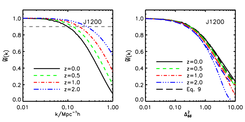
IV.2 The window function
The window function [Eq. (3)] and the normalized one, , are of crucial importance for the following reasons in understanding and reconstructing the velocity field and in improving RSD modeling (Paper I). (1) describes the impact of the nonlinear evolution on the velocity-density relation. (2) quantifies a major systematic error in RSD cosmology. We have shown that the leading term in the redshift space matter power spectrum is . Hence the widely adopted Kaiser formula underestimates by a factor . Perturbation theory predicts a bias at Mpc and (Paper I), much larger than the statistical error associated with stage IV dark energy surveys. (3) behaves as a window function exerting on the density field to reveal the underlying velocity field. This deterministic function can be inferred from RSD in spectroscopic redshift surveys in less model dependent way. So it is essential in three-dimensional peculiar velocity reconstruction in redshift surveys, at cosmological distances.
Figure 5 shows at different redshifts measured in the J1200 simulation. It confirms our theoretical prediction using third-order Eulerian perturbation theory (Paper I), which is applicable at Mpc. As expected, changes from unity at to zero at . As explained in Paper I, quantifies a systematic error in . Since stage IV dark energy surveys have the potential to measure to level accuracy, this -induced systematic error becomes significant, even at relatively high redshift and pretty linear scale Mpc. The situation worsens towards lower redshifts and smaller scales. For example, at . It is already significant for stage III dark energy surveys like BOSS and eBOSS Chuang et al. (2013); Reid et al. (2012b); Tojeiro et al. (2012b). This systematic error may contribute a significant fraction to the tension in between existing measurements and the prediction from Planck cosmology Macaulay et al. (2013).
| Redshift | ||||
|---|---|---|---|---|
| 0.344 | 1.001 | 0.026 | 38 | |
| 0.376 | 1.0 | 0.019 | 54 | |
| 0.416 | 1.001 | 0.012 | 82 | |
| 0.486 | 1.01 | 0.007 | 145 |
We expect the degrees of freedom in is limited. The perturbation theory predicts Bernardeau et al. (2002), for a power law initial power spectrum with power index ,
Here, is the linear matter power spectrum variance and is the nonlinear one. The symbols follow the notation in Bernardeau et al. (2002) and . However, in reality, the power index depends on . So is a function of both and . In this case is often approximated as the effective power index at the nonlinear scale , defined through . Even so, , a function of redshift. On the other hand, the neglected terms of imply a stronger dependence than . These considerations motivate us to propose the following fitting formula:
Notice that we have replaced the linear matter power spectrum with the nonlinear one. Although we still adopt the symbol , it is no longer a prediction from perturbation theory. Instead, it shall be treated as a free function to be fitted against simulation or observation. Nevertheless, from the above argument, we do not expect a strong redshift dependence in .
To check for the above arguments, we plot against (right panel, Fig. 5). Comparing to the - curves in the left panel, we find that the redshift dependence of - curves is greatly reduced. Curves of different redshifts almost overlap with each other at . This behavior suggests that is mainly determined by . Impacts of any other factors should be minor.
![[Uncaptioned image]](/html/1308.0886/assets/x7.png)
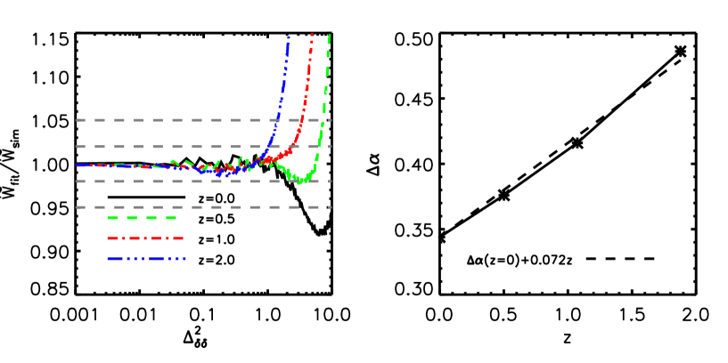
We then obtain the best-fit value of at each redshift. Table 2 lists the best-fit , the associated and reduced . We limit the fitting to , where robust cosmology based on RSD is promising. Furthermore, the proposed fitting formula is not expected to work well at (Fig. 6).
It turns out that the proposed fitting formula works excellently at (Fig. 6). It achieves an accuracy within at scales of interest for RSD cosmology ().
The best-fit varies weakly with redshift. The redshift dependence can be excellently approximated as linear,
| (14) |
with (Fig. 6).
By far we have illustrated the possibility of finding a simple fitting formula to accurately model . We caution that, although the proposed form [Eq. (IV.2)] works very well, it may not necessarily be the best-fitting formula. What we really want to demonstrate here is that has very limited degrees of freedom such that one or two fitting parameters are sufficient to model it to high accuracy. This means that we can efficiently reduce the -induced systematic error without significantly inflating the statistical error in . Whether we can find a more physically motivated and hence more generic and more accurate fitting formula is an issue for further investigation.
IV.3 The velocity correlation function
RSD modeling in Paper I requires information on the velocity correlation function. The correlation function between the th velocity component at position and th velocity component at can be decomposed into two correlation functions and Peebles (1980),
| (15) |
Here is the correlation function of the velocity components along and is the one of velocity components perpendicular to . denote the Cartesian axis. is the pair separation vector.
and do not depend on the choice of coordinate system. The two are not independent. For a potential flow (like and ), we have the textbook result Peebles (1980),
| (16) | |||||
Paper I derives the relation for a curl velocity field like ,
| (17) | |||||
What is relevant for RSD modeling is , assuming the line of sight as the axis. One can easily verify that
| (18) | |||||
One can also prove that
| (19) |
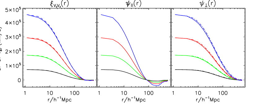
Figure 7 shows the simulated (left column), (middle column) and (right column). It also verifies the above relation (dashed lines in left column). Equations (16) and (17) are also verified against their integral forms [Eq. (16) by dot-dashed lines in right column, Eq. (17) by dotted lines in middle column]:
There are slight deviations in the comparison, likely caused by the simplest trapezoidal rule for integration, or sparse sampling in low- region.
Figure 7 verifies our speculation in Paper I on the correlation lengths of the three velocity components. We see that has the largest correlation length of Mpc, in concordance with the fact that its power spectrum peaks at Mpc. Due to this large correlation length and due to its complete correlation with the density field, its contribution to the redshift space matter power spectrum is the most complicated to model. We refer readers to Paper I for details.
On the contrary, has the smallest Mpc correlation length, which is shorter than scales of interest for RSD cosmology. This motivates us to treat it as an uncorrelated field in our RSD modeling [Eq. (21), paper I]. Its impact on RSD is completely captured by the damping function , which will be quantified later in this paper.
Since a significant fraction of comes from bulk motion, has a correlation length of Mpc, larger than that of . So we have to take into account its self-clustering [e.g., Eq. (25) of paper I].


IV.4 The one-point velocity PDF and cumulants
RSD modeling requires us to quantify the non-Gaussianity of the three velocity components (Paper I). Fig. 8 shows () at different redshifts. For comparison, we also overplot the Gaussian distribution with the same velocity mean (zero) and dispersion. Here, is the corresponding PDF of the velocity component along the -axis.
To better quantify the non-Gaussianity, we calculate the reduced cumulants of the three velocity components, . The calculation is done against the real space velocity components on regular grid points. The real space velocity components are obtained by Inverse Fourier Transforming the Fourier space velocity components on regular gird points. Since the velocity field is symmetrical, . The nonvanishing cumulants are
For Gaussian fields, . But all three velocity components have visible non-Gaussianity ( Fig. 9).
is nearly Gaussian, with at all redshifts. This is consistent with the fact that the dominant contribution comes from linear scales (Fig. 1). However, it may appear to contradict the fact that it is completely correlated with the density field, which is highly nonlinear and non-Gaussian. The reason is that at highly nonlinear scales, and hence it filters away most non-Gaussian contribution.
In contrast, is strongly non-Gaussian (Fig. 9), consistent with the fact that most of its contribution comes from strongly nonlinear and non-Gaussian scales. This result also supports our conclusion that the aliasing effect is subdominant in measured from the G100 simulation, otherwise we may expect a close-to-Gaussian .
The non-Gaussianity of falls somewhere between, with visible departure from Gaussianity in the PDF, and .
An interesting behavior is that, of increase towards lower redshift, while of and decrease (Fig. 9). The increase of non-Gaussianity in indicates that more and more “Gaussian” scales have been converted to be “non-Gaussian” due to the ongoing nonlinear evolution. On the other hand, ongoing virialization in halos and the associated velocity randomization may be responsible for decreasing non-Gaussianity in and .
IV.5 The damping functions
Paper I proves that all three velocity components contribute to the FOG effect. Their contributions are described by the corresponding damping function (Paper I),
The cumulant expansion theorem allows us to express in terms of cumulants (Paper I),
| (21) |
where . is the one-dimensional velocity dispersion,
| (22) |
To the first order, the damping functions take Gaussian form,
| (23) |
It is completely determined by (right panel, Fig. 9).
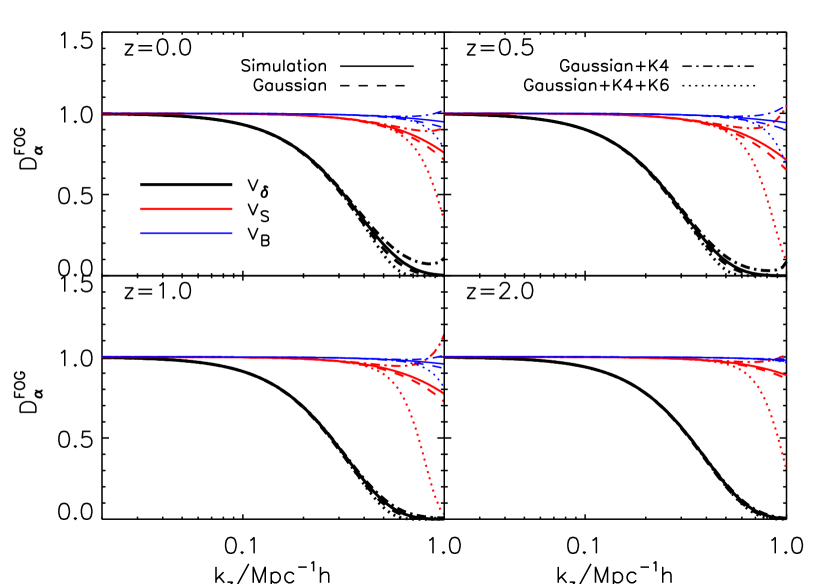
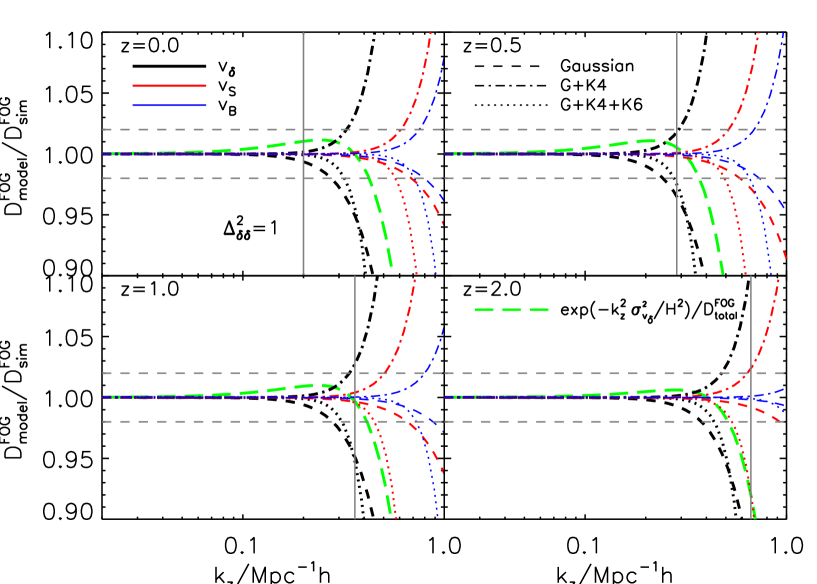
We test the accuracy of Eq. (23) against the exact , calculated from simulations using Eq. (IV.5). Figures 10 and 11 show that Eq. (23) agrees well with the simulation for all three velocity components, for a wide range of . The accuracy is better than where .
Can adding higher-order terms such as and in Eq. (21) improve the modeling accuracy of ? This test is shown in Fig. 10 and Fig. 11. Unfortunately, including or does not necessarily improve the modeling accuracy of . Instead, including these terms often causes unphysical behaviors such as .
We thus conclude that the Gaussian approximation [Eq. (23)] is in practice the optimal approximation of , for all three velocity components. Furthermore, since , to high accuracy we can approximate the overall damping function as
Figure 11 verifies that the last approximation works at accuracy at Mpc and .
The excellent performance of the above Gaussian approximation is very surprising, since much of the literature prefers a Lorentz form (e.g. Peacock and Dodds (1994); Cole et al. (1995); Diaferio and Geller (1996); Bromley et al. (1997)) or more complicated ones (e.g. Kang et al. (2002)). This seems to contradict our findings. The point is that many of these studies infer the damping function by fitting the form against simulations. However, there are ignored high-order corrections inside of the parentheses [refer to Eq. (II); For more details, refer to Paper I]. Ignoring these corrections leads to misinterpretation of FOG. For example, positive high-order corrections can be misinterpreted as a damping function weaker than the Gaussian form. This issue will be further clarified when we quantify the accuracy of the above RSD modeling with simulations.
V Summaries and Discussions
Numerical results presented in the current paper confirm many of our qualitative arguments and speculations in Paper I. (1) They show that dominates over and at Mpc. The field is close to Gaussian, with a correlation length of Mpc. has the largest velocity one-dimension dispersion, km/s at . It not only dominates the large-scale enhancement of redshift space clustering, but also dominates the FOG effect. We also measure a key function and confirm that it can indeed induce underestimation in . We show by an example that has very limited degrees of freedom and can be described by a simple fitting formula accurately. (2) The field is subdominant at Mpc and is negligible at Mpc. It has the smallest velocity dispersion. Due to observed numerical artifacts, we can only obtain the upper limit km/s (). Furthermore, it has the shortest correlation length and can be treated as a random field. Its impact on RSD is fully captured by the damping function . is highly non-Gaussian. However, due to its small amplitude, is well approximated by a Gaussian form at scales of interest. (3) The component is sub-dominant, but non-negligible, at Mpc. km/s at . Its correlation length is of Mpc, so we have to take its clustering into RSD modeling.
There are still many open issues regarding the velocity statistics. Some of them will be addressed in our future works. We just list a few of them here. One immediate question is the halo velocity field. Once we understand it, we can understand the galaxy velocity field with the help of halo model. This piece of information is essential to model the galaxy RSD. Another issue is cosmological dependences of these velocity statistics. An associated question is the information budget in each velocity component, as a function of redshift and scale.
VI Acknowledgements
We thank Jiawei Shao and Yu Yu for useful discussions. This work was supported by the National Science Foundation of China (Grants No. 11025316, No. 11121062, No. 10873035, No. 1133003, No. 10873027, No. 11121062, and No. 11233005), the National Basic Research Program of China (973 Program) under Grant No. 2009CB24901 and the CAS/SAFEA International Partnership Program for Creative Research Teams (KJCX2-YW-T23).
Appendix A Testing the NP method
The NP (Nearest-Particle) method we proposed is simple and straightforward to implement. Despite its simplicity, we argue that it is robust in a number of ways and is hence sufficiently accurate for the statistics presented in this paper. We will run a number of convergence tests to demonstrate its robustness. We will also quantify its accuracy for a number of fiducial velocity fields, which resemble realistic velocity fields.
A.1 The convergence tests
The convergence tests we consider are as follows: (1) Convergence between the three simulations. J1200, J300 and G100 all have particles, but have different box sizes and mass resolutions. By comparing the three simulations, we can estimate the reliable range of the simulated velocity field. (2) Convergence against the grid size. We assign properties of simulation particles to regular grids in order to do Ffast Fourier transformation (FFT). The price to pay is that information at subgrid scales is smoothed out. Furthermore, as an approximated way of sampling the velocity field, it can cause misidentification of different velocity components. For example, finite grids are known to cause spurious Pueblas and Scoccimarro (2009). By varying the grid number and checking for the convergence, we can figure out suitable grid choices and a reliable range of the measured velocity statistics. (3) Sampling bias. The issues addressed in (1) and (2) can be regarded as sampling biases. But throughout the paper we refer to the sampling bias as that caused by the fact that we only have velocity where there are particles. By sampling the velocity field using only a fraction of particles, we amplify this sampling bias. Observing its dependence with respect to the fraction of particles, we can estimate this sampling bias. In particular, if the measured velocity statistics converge when the used fraction of particles is above a certain value, we will have reasonable confidence on the velocity statistics using all particles.
We only show test results at , where numerical artifacts are the most severe. Furthermore, we mainly test the convergence in the power spectrum. The convergence tests can be extended to other statistics.
A.1.1 Comparison between the three simulations
Simulation box size determines the lower limit of reliable range of , while mass resolution determines the upper limit of reliable range of .
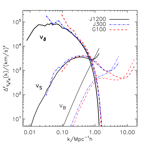
Figure 12 plots () calculated respectively from J1200, J300 and G100. It shows various spurious behaviors and various discrepancies between these simulations. These are manifests of numerical artifacts. In particular, decreases rapidly with increasing resolution from J1200 to G100. This is consistent with the finding in Pueblas and Scoccimarro (2009). Further tests, especially that in Sec. A.2, will identify the origin of this numerical artifact. Figure 12 implies by naive scaling that, simulations of Gpc box size and particles are needed to fully control these numerical artifacts. Although a daunting task, such simulation is within the capability of state of art computation.
Nevertheless, J1200/J300/G100 do converge here and there, where we expect the simulation results to be reliable. Figure 12 (and figures hereafter) implies that, combining these simulations, it is feasible to reliably measure the power spectrum of the three velocity fields in the range of interest (Mpc). In this paper, we combine J1200 at Mpc and G100 at Mpc to measure and . We use G100 to calculate .
For other statistics such as the one-point PDFs, cumulants, and the damping functions, different scales mix and we have difficulty combining these simulations. To address this, we take a simplified approach. Since the power of peaks at /Mpc where J1200 is the most reliable, we only use J1200 to measure statistics of . Both the power of and peak at Mpc where G100 is most reliable, so we use G100 to measure statistics of .
A.1.2 Grid size
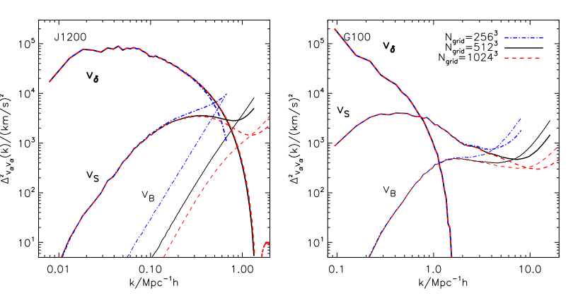
We calculate the power spectrum by assigning particle properties (mass, velocity, etc.) onto regular gird points and performing FFT. A natural convergence test is then against the grid size . Figure 13 shows () calculated in the J1200 and G100 simulations respectively, with . (1) Convergence tests with J1200 show that grid-size-associated numerical artifacts in are negligible at Mpc, for grid size Mpc (). They are negligible at Mpc, for grid size Mpc (). Convergence tests with G100 show that numerical artifacts in associated with grid size are negligible at Mpc, for grid size Mpc (). (2) J1200 and G100 show that grid-size-associated numerical artifacts in are negligible at (, , ), for (, , ). (3) Convergence tests with G100 show that, to reliably measure to Mpc, grid size Mpc is required. To reach Mpc, Mpc is required. We are then able to conclude that, the measured power spectra shown in Fig. 1 are robust against numerical artifacts associated with nonzero grid size (finite grid number).
Nonetheless, we do find significant disagreement between different grid sizes over some ranges in Fig. 13. These are clear manifestation of significant numerical artifacts associated with grid size. The situation is the most severe for . No convergence is found in J1200, meaning that even with Mpc, it is not sufficient to accurately sample the field. Tests with G100 show that Mpc is needed to accurately measure at Mpc.
There are at least three types of numerical artifacts associated with grid size: (1) One is the smoothing effect, suppression of small-scale power caused by the assignment window function (e.g., Jing (2005) and references therein). (2) Another is the alias effect caused by finite grid number. It causes mixture of power among wave vectors Jing (2005). Here is the Nyquist wave number and is the grid size. is the three-dimensional integer vector. These two biases also exist for the matter power spectrum measurement. (3) For the velocity measurement, there is another type of alias effect. It causes mixture between different velocity components Pueblas and Scoccimarro (2009). This effect is especially severe for measurement.
All three types of bias depend on the grid size (number). The assignment window function for the NP method is . Here is the position of the given grid point and is the location of the corresponding nearest particle. Notice that this window function is inhomogeneous. Namely, it is not completely determined by . So the formula of alias effect, derived with the condition in Jing (2005), does not apply here. It is beyond the scope of this paper to derive a general expression of the alias effect. Instead, we work on a limiting case of infinite particle number density (). Under this limit, and . Following Jing (2005), we obtain
| (25) |
Under this limit, the smoothing effect vanishes (the prefactor of the power spectrum at is unity). The alias effect, on one hand, shows as contaminations from modes with to the measure mode. On the other hand, it shows as leakages between different velocity components (, , ). Sec. A.2 will quantify these leakages. Both alias effects contribute to the decreasing of power at small scales in both and (Fig. 13).
These convergence tests show that, by combining J1200/J300/G100 we can safely neglect the smoothing and aliasing caused by nonzero grid size at scale of interest. So we do not attempt to correct for these numerical artifacts. For methods of correcting them, refer to Jing (2005); Pueblas and Scoccimarro (2009); Koda et al. (2013); Cui et al. (2008).
A.1.3 Sampling bias
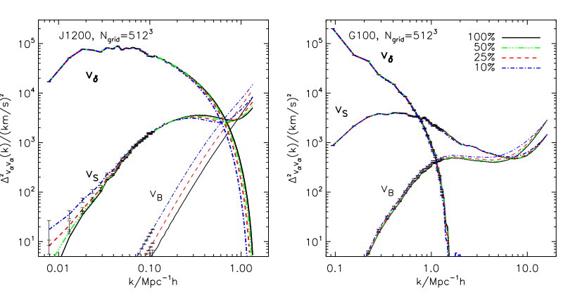

To highlight the sampling bias, we randomly select , , and of the simulation particles and compare the measured velocity power spectra with those of particles (Fig. 14). A complexity is that, the assignment window function of the NP method is particle number density dependent. So reducing the number of particles sampled also changes the alias effect. Hence the numerical artifacts shown in Fig. 14 should be a mixture of sampling bias and alias effect. We do not attempt to separate the two in this paper.
For J1200, the power spectra of and converge at Mpc. At Mpc, the results vary between the four cases (, , , and ). We then know that particles are not sufficient to simulate and at Mpc. However, we do not know if particles are sufficient. The situation for is much worse. The power of decreases with increasing number density at all scales. This again confirms that the measured in J1200 is mainly numerical artifact, instead of real signal.
For G100, convergences are much better, since the sampling bias should decreases rapidly towards higher particle number density. These convergences tell us that sampling bias in a G100 like simulation with particles and /Mpc box is negligible at Mpc for all the three velocity components.
Figure 15 shows correlation functions under the same conditions. It shows that the NP method gives considerably accurate estimations for and , but overestimates . This is consistent with the large discrepancies in at large in Fig. 14. It is hence challenging to accurately simulate . A good thing is that, in our RSD modeling, can be chosen as a free parameter to be fitted or even set as zero. So the inability of accurately simulating is not a severe problem.
A.2 Testing against velocity fields of known statistics
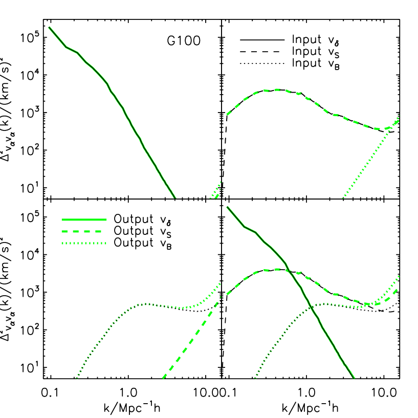
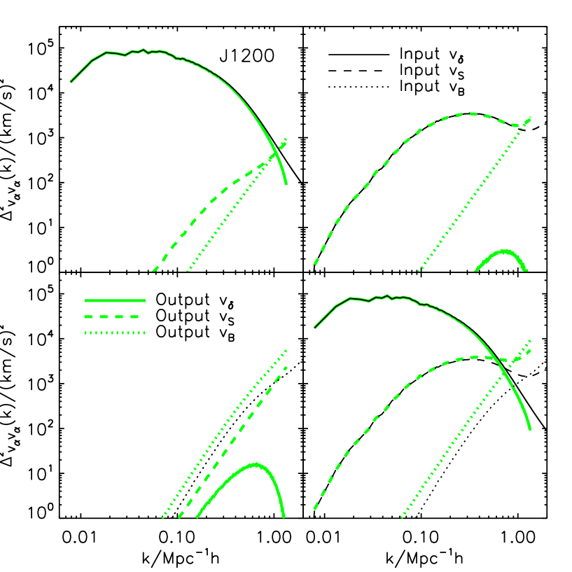
The above convergence tests are good at diagnosing and setting up the lower limit of some numerical artifacts. But they can be blind for other artifacts and can have trouble disentangling various numerical artifacts. A complementary test can be done with a fiducial velocity field of known statistics (in our case the power spectrum). By comparing the measured statistics with the input statistics, errors in the measurement can be quantified straightforwardly. Obviously these errors depend on the fiducial input. So the crucial step for this test is the construction of the input velocity field as realistic as possible. Our proposed velocity decomposition makes this step simpler and more robust. This allows us to perform rigorous tests of the NP method.
First we construct fiducial velocity fields of known statistics on regular grid points. The fiducial is constructed by a combination of measured density field and the best fitted window function in §IV.2, . The fiducial can be generated using the measured power spectra, if we assume Gaussianity. Alternatively, we can directly use the measured fields by the NP method on regular grid points from our simulations. We will adopt this second approach.
Secondly we assign each particle a velocity, which is the velocity of its nearest grid point. Along with the particle positions from the corresponding simulation (J1200/J300/G100), this is the new “simulation” we use to test our NP method. We will assign these velocities to grid points to do the test. By setting some of the velocity components to zero, we can generate up to seven velocity fields. We have tested the following four cases of them. (A) but and ; (B) but and ; (C) , but and ; and (D) , and .
Tests on J1200 are shown in Fig. 16. (1) First we focus on the measurement accuracy in . Test on case A shows that the measured agrees well with the input one at Mpc (top left panel, Fig. 16). Tests on case B and C show that the leakages from and to are negligible. So the measured at Mpc is reliable. This is consistent with the results of convergence tests. (2) For , more careful interpretation should be given. Test on case B shows that the measured agrees well with the input one at Mpc (top right panel, Fig. 16). However, tests on case A and case C show that the leakage and are significant. Case D shows that we should only trust the measurement at Mpc. This is again consistent with findings through the convergence test. (3) Test on case C shows that the measured agrees with the input one, within a factor of 2 (bottom left panel, Fig. 16). However, this result is very misleading. Tests on case A and B shows that most of the output is caused by the leakage and . In other words, measured in the J1200 simulation is mainly noise, instead of real signal. This is consistent with our previous conclusion based on the convergence tests.
Tests on G100 are shown in Fig. 17. By similar argument, we can draw the conclusion that the NP method is accurate to measure and at Mpc. Now the measurement on is significantly improved, since the leakages and are both subdominant at Mpc.
These tests can be used to calibrate errors in the velocity measurement. For example, by adding the power spectra of and in case A to that of measured from the real data, one can improve the measurement of the power spectrum.
References
- Zhang et al. (2013) P. Zhang, J. Pan, and Y. Zheng, Phys. Rev. D 87, 063526 (2013), eprint 1207.2722.
- Jackson (1972) J. C. Jackson, MNRAS 156, 1P (1972).
- Sargent and Turner (1977) W. L. W. Sargent and E. L. Turner, ApJL 212, L3 (1977).
- Peebles (1980) P. J. E. Peebles, The large-scale structure of the universe (1980).
- Kaiser (1987) N. Kaiser, MNRAS 227, 1 (1987).
- Peacock and Dodds (1994) J. A. Peacock and S. J. Dodds, MNRAS 267, 1020 (1994), eprint arXiv:astro-ph/9311057.
- Ballinger et al. (1996) W. E. Ballinger, J. A. Peacock, and A. F. Heavens, MNRAS 282, 877 (1996), eprint arXiv:astro-ph/9605017.
- Peacock et al. (2001) J. A. Peacock, S. Cole, P. Norberg, C. M. Baugh, J. Bland-Hawthorn, T. Bridges, R. D. Cannon, M. Colless, C. Collins, W. Couch, et al., Nature (London) 410, 169 (2001), eprint arXiv:astro-ph/0103143.
- Tegmark et al. (2002) M. Tegmark, A. J. S. Hamilton, and Y. Xu, MNRAS 335, 887 (2002), eprint arXiv:astro-ph/0111575.
- Tegmark et al. (2004) M. Tegmark, M. R. Blanton, M. A. Strauss, F. Hoyle, D. Schlegel, R. Scoccimarro, M. S. Vogeley, D. H. Weinberg, I. Zehavi, A. Berlind, et al., Astrophys. J. 606, 702 (2004), eprint arXiv:astro-ph/0310725.
- Amendola et al. (2005) L. Amendola, C. Quercellini, and E. Giallongo, MNRAS 357, 429 (2005), eprint arXiv:astro-ph/0404599.
- Linder (2005) E. V. Linder, Phys. Rev. D 72, 043529 (2005), eprint arXiv:astro-ph/0507263.
- Yamamoto et al. (2005) K. Yamamoto, B. A. Bassett, and H. Nishioka, Physical Review Letters 94, 051301 (2005), eprint arXiv:astro-ph/0409207.
- Zhang et al. (2007) P. Zhang, M. Liguori, R. Bean, and S. Dodelson, Physical Review Letters 99, 141302 (2007), eprint 0704.1932.
- Guzzo et al. (2008) L. Guzzo, M. Pierleoni, B. Meneux, E. Branchini, O. Le Fèvre, C. Marinoni, B. Garilli, J. Blaizot, G. De Lucia, A. Pollo, et al., Nature (London) 451, 541 (2008), eprint 0802.1944.
- Wang (2008) Y. Wang, JCAP 5, 21 (2008), eprint 0710.3885.
- Percival and White (2009) W. J. Percival and M. White, MNRAS 393, 297 (2009), eprint 0808.0003.
- Song and Percival (2009) Y.-S. Song and W. J. Percival, JCAP 10, 4 (2009), eprint 0807.0810.
- White et al. (2009) M. White, Y.-S. Song, and W. J. Percival, MNRAS 397, 1348 (2009), eprint 0810.1518.
- Song (2011) Y.-S. Song, Phys. Rev. D 83, 103009 (2011), eprint 1009.2753.
- Wang et al. (2010) Y. Wang, W. Percival, A. Cimatti, P. Mukherjee, L. Guzzo, C. M. Baugh, C. Carbone, P. Franzetti, B. Garilli, J. E. Geach, et al., MNRAS 409, 737 (2010), eprint 1006.3517.
- Blake et al. (2011) C. Blake, S. Brough, M. Colless, C. Contreras, W. Couch, S. Croom, T. Davis, M. J. Drinkwater, K. Forster, D. Gilbank, et al., MNRAS 415, 2876 (2011), eprint 1104.2948.
- Samushia et al. (2012) L. Samushia, W. J. Percival, and A. Raccanelli, MNRAS 420, 2102 (2012), eprint 1102.1014.
- Blake et al. (2012) C. Blake, S. Brough, M. Colless, C. Contreras, W. Couch, S. Croom, D. Croton, T. Davis, M. J. Drinkwater, K. Forster, et al., ArXiv e-prints (2012), eprint 1204.3674.
- Reid et al. (2012a) B. A. Reid, L. Samushia, M. White, W. J. Percival, M. Manera, N. Padmanabhan, A. J. Ross, A. G. Sánchez, S. Bailey, D. Bizyaev, et al., ArXiv e-prints (2012a), eprint 1203.6641.
- Tojeiro et al. (2012a) R. Tojeiro, W. J. Percival, J. Brinkmann, J. R. Brownstein, D. Eisenstein, M. Manera, C. Maraston, C. K. McBride, D. Duna, B. Reid, et al., ArXiv e-prints (2012a), eprint 1203.6565.
- Jain and Zhang (2008) B. Jain and P. Zhang, Phys. Rev. D 78, 063503 (2008), eprint 0709.2375.
- Linder (2008) E. V. Linder, Astroparticle Physics 29, 336 (2008), eprint 0709.1113.
- Reyes et al. (2010) R. Reyes, R. Mandelbaum, U. Seljak, T. Baldauf, J. E. Gunn, L. Lombriser, and R. E. Smith, Nature (London) 464, 256 (2010), eprint 1003.2185.
- Cai and Bernstein (2012) Y.-C. Cai and G. Bernstein, MNRAS 422, 1045 (2012), eprint 1112.4478.
- Gaztañaga et al. (2012) E. Gaztañaga, M. Eriksen, M. Crocce, F. J. Castander, P. Fosalba, P. Marti, R. Miquel, and A. Cabré, MNRAS 422, 2904 (2012), eprint 1109.4852.
- Jennings et al. (2012) E. Jennings, C. M. Baugh, B. Li, G.-B. Zhao, and K. Koyama, ArXiv e-prints (2012), eprint 1205.2698.
- Li et al. (2013) B. Li, W. A. Hellwing, K. Koyama, G.-B. Zhao, E. Jennings, and C. M. Baugh, MNRAS 428, 743 (2013), eprint 1206.4317.
- Schlegel et al. (2011) D. Schlegel, F. Abdalla, T. Abraham, C. Ahn, C. Allende Prieto, J. Annis, E. Aubourg, M. Azzaro, S. B. C. Baltay, C. Baugh, et al., ArXiv e-prints (2011), eprint 1106.1706.
- Laureijs et al. (2011) R. Laureijs, J. Amiaux, S. Arduini, J. . Auguères, J. Brinchmann, R. Cole, M. Cropper, C. Dabin, L. Duvet, A. Ealet, et al., ArXiv e-prints (2011), eprint 1110.3193.
- Scoccimarro (2004) R. Scoccimarro, Phys. Rev. D 70, 083007 (2004), eprint arXiv:astro-ph/0407214.
- Seljak and McDonald (2011) U. Seljak and P. McDonald, JCAP 11, 39 (2011), eprint 1109.1888.
- Okumura et al. (2012a) T. Okumura, U. Seljak, P. McDonald, and V. Desjacques, JCAP 2, 10 (2012a), eprint 1109.1609.
- Okumura et al. (2012b) T. Okumura, U. Seljak, and V. Desjacques, JCAP 11, 014 (2012b), eprint 1206.4070.
- Bonoli and Pen (2009) S. Bonoli and U. L. Pen, MNRAS 396, 1610 (2009), eprint 0810.0273.
- Desjacques and Sheth (2010) V. Desjacques and R. K. Sheth, Phys. Rev. D 81, 023526 (2010), eprint 0909.4544.
- (42) BigBoss/MS-DESI, URL http://bigboss.lbl.gov/.
- (43) CHIME, URL http://chime.phas.ubc.ca/.
- (44) Euclid, URL http://www.euclid-ec.org/.
- (45) SKA, URL http://www.skatelescope.org/.
- Jing et al. (2007) Y. P. Jing, Y. Suto, and H. J. Mo, Astrophys. J. 657, 664 (2007), eprint arXiv:astro-ph/0610099.
- Springel et al. (2001) V. Springel, N. Yoshida, and S. D. M. White, New Astronomy 6, 79 (2001), eprint arXiv:astro-ph/0003162.
- Springel (2005) V. Springel, MNRAS 364, 1105 (2005), eprint arXiv:astro-ph/0505010.
- Bernardeau and van de Weygaert (1996) F. Bernardeau and R. van de Weygaert, MNRAS 279, 693 (1996).
- van de Weygaert and Schaap (2009) R. van de Weygaert and W. Schaap, in Data Analysis in Cosmology, edited by V. J. Martínez, E. Saar, E. Martínez-González, and M.-J. Pons-Bordería (2009), vol. 665 of Lecture Notes in Physics, Berlin Springer Verlag, pp. 291–413.
- Pueblas and Scoccimarro (2009) S. Pueblas and R. Scoccimarro, Phys. Rev. D 80, 043504 (2009), eprint 0809.4606.
- Bernardeau et al. (2002) F. Bernardeau, S. Colombi, E. Gaztañaga, and R. Scoccimarro, Physics reports 367, 1 (2002), eprint arXiv:astro-ph/0112551.
- Chuang et al. (2013) C.-H. Chuang, F. Prada, A. J. Cuesta, D. J. Eisenstein, E. Kazin, N. Padmanabhan, A. G. Sanchez, X. Xu, F. Beutler, M. Manera, et al., ArXiv e-prints (2013), eprint 1303.4486.
- Reid et al. (2012b) B. A. Reid, L. Samushia, M. White, W. J. Percival, M. Manera, N. Padmanabhan, A. J. Ross, A. G. Sánchez, S. Bailey, D. Bizyaev, et al., MNRAS 426, 2719 (2012b), eprint 1203.6641.
- Tojeiro et al. (2012b) R. Tojeiro, W. J. Percival, J. Brinkmann, J. R. Brownstein, D. J. Eisenstein, M. Manera, C. Maraston, C. K. McBride, D. Muna, B. Reid, et al., MNRAS 424, 2339 (2012b), eprint 1203.6565.
- Macaulay et al. (2013) E. Macaulay, I. Kathrine Wehus, and H. K. Eriksen, ArXiv e-prints (2013), eprint 1303.6583.
- Cole et al. (1995) S. Cole, K. B. Fisher, and D. H. Weinberg, MNRAS 275, 515 (1995), eprint arXiv:astro-ph/9412062.
- Diaferio and Geller (1996) A. Diaferio and M. J. Geller, Astrophys. J. 467, 19 (1996), eprint arXiv:astro-ph/9602086.
- Bromley et al. (1997) B. C. Bromley, M. S. Warren, and W. H. Zurek, Astrophys. J. 475, 414 (1997), eprint arXiv:astro-ph/9701177.
- Kang et al. (2002) X. Kang, Y. P. Jing, H. J. Mo, and G. Börner, MNRAS 336, 892 (2002), eprint arXiv:astro-ph/0201124.
- Jing (2005) Y. P. Jing, Astrophys. J. 620, 559 (2005), eprint arXiv:astro-ph/0409240.
- Koda et al. (2013) J. Koda, C. Blake, T. Davis, M. Scrimgeour, G. B. Poole, and L. S. Smith, ArXiv e-prints (2013), eprint in preparation.
- Cui et al. (2008) W. Cui, L. Liu, X. Yang, Y. Wang, L. Feng, and V. Springel, Astrophys. J. 687, 738 (2008), eprint 0804.0070.