aainstitutetext: Faculty of Physics, University of Bielefeld, D-33615 Bielefeld, Germanybbinstitutetext: Department of Physics, Norwegian University of Science and Technology,
N-7491 Trondheim, Norway
ccinstitutetext: Department of Physics, Kent State University, Kent OH 44242 USAddinstitutetext: Department of Physics and Helsinki Institute of Physics, P. O. Box 64, FI-00014 University of Helsinki, Finland

Equation of State of hot and dense QCD: Resummed perturbation theory confronts lattice data

Sylvain Mogliacci b    Jens O. Andersen c    Michael Strickland a    Nan Su d    and Aleksi Vuorinen sylvain@physik.uni-bielefeld.de andersen@tf.phys.ntnu.no mstrick6@kent.edu nansu@physik.uni-bielefeld.de aleksi.vuorinen@helsinki.fi
Abstract

We perform a detailed analysis of the predictions of resummed perturbation theory for the pressure and the second-, fourth-, and sixth-order diagonal quark number susceptibilities in a hot and dense quark-gluon plasma. First, we present an exact one-loop calculation of the equation of state within hard-thermal-loop perturbation theory (HTLpt) and compare it to a previous one-loop HTLpt calculation that employed an expansion in the ratios of thermal masses and the temperature. We find that this expansion converges reasonably fast. We then perform a resummation of the existing four-loop weak coupling expression for the pressure, motivated by dimensional reduction. Finally, we compare the exact one-loop HTLpt and resummed dimensional reduction results with state-of-the-art lattice calculations and a recent mass-expanded three-loop HTLpt calculation.

Keywords:
Quark-Gluon Plasma, Resummation
preprint: BI-TP 2013/17arxiv: 1307.8098

1 Introduction

Understanding the behavior of strongly interacting matter subject to extreme conditions is important in many physical contexts such as the study of the early universe and the interiors of compact stars. The determination of the QCD phase diagram has subsequently received considerable attention over the past few decades. On the experimental side, an enormous effort has gone to the creation of the quark-gluon plasma (QGP) in heavy ion collisions, most recently carried out at the Relativistic Heavy Ion Collider (RHIC) of Brookhaven Tannenbaum , and at the Large Hadron Collider (LHC) of CERN Muller . On the theoretical side, both lattice gauge theory and model calculations have been employed to map out the phase diagram of QCD and in particular locate a possible critical end point of a line of first order phase transitions (see e.g. Satz for a review).

Unfortunately, at nonzero quark chemical potentials μfsubscript𝜇𝑓\mu_{f}, lattice Monte Carlo simulations are hampered by the infamous sign problem related to the complex nature of the lattice action, rendering importance sampling techniques inapplicable. One of the proposed ways to circumvent this problem — and thus enter the μ𝜇\muT𝑇T plane — is by Taylor expanding various physical quantities in powers of the ratios μf/Tsubscript𝜇𝑓𝑇\mu_{f}/T and evaluating the coefficients at μf=0subscript𝜇𝑓0\mu_{f}=0. As these derivatives are evaluated at zero density, they can be computed on the lattice using standard techniques. In the case of the pressure, the coefficients are called quark number susceptibilities (QNS), which indeed carry information about the response of the system to nonzero baryon density as well as correlations between different quark flavors.

Let us denote by 𝝁𝝁\bm{\mu} an Nfsubscript𝑁fN_{\mbox{\scriptsize f}} - component vector consisting of the quark chemical potentials for the different flavors, 𝝁(μ1,μ2,,μNf)𝝁subscript𝜇1subscript𝜇2subscript𝜇subscript𝑁f\bm{\mu}\equiv(\mu_{1},\mu_{2},...,\mu_{N_{\mbox{\scriptsize f}}}), with Nfsubscript𝑁fN_{\mbox{\scriptsize f}} being typically 2 or 3 at the relevant energies. We can then define the QNS, χijk(T)subscript𝜒𝑖𝑗𝑘𝑇\chi_{ijk}\left(T\right), simply as derivatives of the pressure p(T,𝝁)𝑝𝑇𝝁p\left(T,\bm{\mu}\right), according to

χijk(T)subscript𝜒𝑖𝑗𝑘𝑇\displaystyle\chi_{ijk}\left(T\right) \displaystyle\equiv i+j+k+p(T,𝝁)μuiμdjμsk|𝝁=0,evaluated-atsuperscript𝑖𝑗𝑘𝑝𝑇𝝁superscriptsubscript𝜇𝑢𝑖superscriptsubscript𝜇𝑑𝑗superscriptsubscript𝜇𝑠𝑘𝝁0\displaystyle\frac{\partial^{i+j+k+...}\;p\left(T,\bm{\mu}\right)}{\partial\mu_{u}^{i}\,\partial\mu_{d}^{j}\,\partial\mu_{s}^{k}\,...}\bigg{|}_{\bm{\mu}=0}\,, (1)

where the indices u,d,s𝑢𝑑𝑠u,\,d,\,s\,... refer to the quark flavors. The determination of the equation of state (EoS) in the μ𝜇\muT𝑇T plane is then limited only by the convergence of the corresponding series in powers of μf/Tsubscript𝜇𝑓𝑇\mu_{f}/T, i.e. ultimately by the magnitudes of the QNS. Recent studies of these quantities on the lattice can be found e.g. in refs. bieleHighT ; biele1 ; biele2 ; bazavov12 ; wuppertalcharge ; chi4 . In addition, lattice studies of two-color QCD with an even number of flavors, which does not suffer from the sign problem, have been performed at high density in refs. HandsNc2_1 ; HandsNc2_2 .

Due to the difficulties in performing lattice simulations far above the pseudo-critical deconfinement transition temperature Tcsubscript𝑇cT_{\mbox{\scriptsize c}} (recalling the crossover nature of the transition at μf=0subscript𝜇𝑓0\mu_{f}=0), it is important to have complementary techniques that can bridge the gap between low and high temperatures. In this context, analytic weak coupling techniques are clearly the method of choice, as they work optimally at asymptotically high temperatures and can be fairly easily continued to the vicinity of the transition region. In recent years, there have been numerous analytic calculations of the chemical potential dependence of the pressure as well as the QNS, using techniques such as unresummed perturbation theory aleksi1 ; aleksi2 ; aleksi3 ; ipp3 , various hard-thermal-loop motivated approaches blaizot1 ; blaizot2 ; mustafa1 ; mustafa2 ; mustafa3 , hard-thermal-loop perturbation theory (HTLpt) baierredlich ; JensMike1 ; sylvain1 ; mikehaque ; Haque1 ; haque , the large-Nfsubscript𝑁fN_{\mbox{\scriptsize f}} limit of QCD ipp1 ; ipp2 , and even the gauge/gravity duality in the context of strongly coupled large-Ncsubscript𝑁cN_{\mbox{\scriptsize c}}\ 𝒩=4𝒩4{\mathcal{N}}=4 Super Yang-Mills theory ads . Finally, similar investigations have also been carried out using various field theoretical PNJL1 ; ModelForQCD2 ; PNJL3 and holographic Jinfeng models of QCD.

In ref. sylvain1 , four of the present authors applied both HTLpt and a resummation scheme motivated by dimensional reduction (DR) to determine the second- and fourth-order diagonal QNS of hot QCD. The calculation involving HTLpt was carried out only to one-loop order, and moreover utilized an expansion in the ratio m/T𝑚𝑇m/T, where m𝑚m represents both the Debye and quark thermal masses of order gT𝑔𝑇gT. A similar technique was recently further employed to two-loop order in refs. mikehaque ; Haque1 as well as to three-loop order in haque , exhibiting sizable devitations from the results of sylvain1 . Motivated by these developments, our aim in the current paper is to continue the work of sylvain1 in three directions:

  • Carry out an exact one-loop HTLpt calculation with no m/T𝑚𝑇m/T-expansion, thereby analyzing the convergence of the expansion and the validity of the corresponding expanded results.

  • Generalize all of our previous results, both within one-loop HTLpt and four-loop DR, to the sixth order quark number susceptibility as well as the chemical potential dependence of the pressure itself, covering also the case of Nf=2subscript𝑁f2N_{\mbox{\scriptsize f}}=2.

  • Perform a careful explicit comparison of our results with state-of-the-art lattice data, and to the three-loop HTLpt results of haque , when possible.

The first of these points is particularly important, because it provides a highly nontrivial quantitative check of one of the crucial analytic approximations used in HTLpt calculations, namely the m/T𝑚𝑇m/T-expansion, which in fact is an essential ingredient in all higher order computations within HTLpt. Its convergence has been studied in scalar ϕ4superscriptitalic-ϕ4\phi^{4} theory to three-loop order motspt with encouraging results; however, to our knowledge, our study is the first calculation to probe such an m/T𝑚𝑇m/T-expansion within QCD.

Our paper is organized as follows. In section 2, we briefly describe hard-thermal-loop perturbation theory and dimensional reduction as two ways of reorganizing perturbative expansions within thermal QCD. We also outline the computation of the exact one-loop and partial four-loop pressures in these two setups, respectively. In section 3, we investigate the convergence of the m/T𝑚𝑇m/T- expansion for the one-loop HTLpt results. In section 4, we compare our results with the three-loop HTLpt calculation haque as well as to lattice data. Finally, in section 5 we draw our conclusions. Nearly all of the computational details have been relegated to the appendices. In appendix A, we first explain our notation, in appendix B, we list the matching coefficients of Electrostatic QCD (EQCD) needed in the derivation of the four-loop EoS within DR, and in appendix C we present a detailed evaluation of the exact one-loop HTLpt pressure. Finally, in appendix D, we provide some computational details regarding the branch cut discontinuities that are encountered in exact HTLpt calculations, and in appendix E, we go through the derivation of the m/T𝑚𝑇m/T- expansion employed in ref. sylvain1 .

We would like to point out that all calculations presented in this paper have been carried out in the limit of vanishing bare quark masses. In the case of our DR calculation, we have explicitly checked that this only affects the results in any noticeable way at the very lowest temperatures shown, where the validity of perturbation theory is in any case questionable. As for HTLpt, a study of the mass dependence of the one-loop quark self-energy and gluon polarization functions has been carried out in Seipt1 , indicating that a similar conclusion should hold also in this case.

2 Resummations in thermal QCD

The (bare) Lagrangian density of massless QCD reads

QCDsubscriptQCD\displaystyle{\cal L}_{\rm QCD} =\displaystyle= 12Tr[GμνGμν]+iψ¯γμDμψ+gf+gh,12Trdelimited-[]subscript𝐺𝜇𝜈superscript𝐺𝜇𝜈𝑖¯𝜓superscript𝛾𝜇subscript𝐷𝜇𝜓subscriptgfsubscriptgh\displaystyle-\frac{1}{2}{\rm Tr}[G_{\mu\nu}\,G^{\mu\nu}]+i\bar{\psi}\gamma^{\mu}D_{\mu}\psi+{\cal L}_{\rm gf}+{\cal L}_{\rm gh}\,, (2)

in which the gluon field strength tensor is defined by Gμν=μAννAμig[Aμ,Aν]superscript𝐺𝜇𝜈superscript𝜇superscript𝐴𝜈superscript𝜈superscript𝐴𝜇𝑖𝑔superscript𝐴𝜇superscript𝐴𝜈G^{\mu\nu}=\partial^{\mu}A^{\nu}-\partial^{\nu}A^{\mu}-ig[A^{\mu},A^{\nu}] and the covariant derivative in the fundamental representation by Dμ=μigAμsuperscript𝐷𝜇superscript𝜇𝑖𝑔superscript𝐴𝜇D^{\mu}=\partial^{\mu}-igA^{\mu}, while the term involving the quark fields ψ𝜓\psi contains an implicit sum over the Nfsubscript𝑁fN_{\mbox{\scriptsize f}} quark flavors. The ghost term ghsubscriptgh{\cal L}_{\rm gh} depends on the gauge-fixing term gfsubscriptgf{\cal L}_{\rm gf}; in the present work, we employ the general covariant gauge, where the latter reads

gfsubscriptgf\displaystyle{\cal L}_{\rm gf} =\displaystyle= 1ξTr[(μAμ)2],1𝜉Trdelimited-[]superscriptsubscript𝜇superscript𝐴𝜇2\displaystyle-\frac{1}{\xi}{\rm Tr}[(\partial_{\mu}A^{\mu})^{2}]\,, (3)

with ξ𝜉\xi standing for the gauge-fixing parameter.

Computing various thermodynamic quantities within entirely unresummed (‘naive’ or diagrammatic) perturbation theory amounts to expanding them in power series organized by even powers of the coupling constant g𝑔g, letting the renormalization of the coupling (and possibly quark masses) cancel the 1/ϵ1italic-ϵ1/\epsilon ultraviolet (UV) divergences encountered.111We work within dimensional regularization, so all of our integrals are defined in d=32ϵ𝑑32italic-ϵd=3-2\epsilon spatial dimensions. This procedure, which amounts to an expansion around an ideal gas of massless quasiparticles, however typically runs into difficulties with physical infrared (IR) divergences already at low loop orders, necessitating some type of a physically motivated resummation of higher-loop Feynman diagrams to be carried out. This may be done in a way, in which one always expands the final n𝑛n-loop result to order g2(n1)superscript𝑔2𝑛1g^{2(n-1)}, dropping all “extra” terms from the result before evaluating it numerically. Such a procedure has, however, been seen to lead to rather poor convergence of different observables, and to this end, several different resummation schemes accounting for some higher order contributions have been proposed (see e.g. blaizot3 ; kraemmer1 ; JensMike2 for reviews).

In the remainder of this section, we will introduce two ways of curing the IR problems encountered in thermal QCD calculations, involving the resummation of certain classes of higher order diagrams. These include firstly hard-thermal-loop perturbation theory, where the expansion point of perturbation theory is shifted to an ideal gas of massive quasiparticles, providing a marked improvement in the convergence properties of weak coupling expansion. At the same time, the physical idea of dimensional reduction can be seen to suggest a highly natural way of including certain higher order contributions to different equilibrium quantities, employing a weak coupling expansion within the effective theory Electrostatic QCD (EQCD). As our presentation will no doubt be rather superficial, we refer the interested reader to the original references Jens2 ; Jens3 ; braaten2 ; Kajantie1 for more details about both of these topics.

2.1 Hard-thermal-loop perturbation theory

Within HTLpt, the reorganization of the perturbative expansion is achieved by writing the Lagrangian density of QCD in the form

HTLptsubscriptHTLpt\displaystyle{\cal L_{\rm HTLpt}} =\displaystyle= (QCD+HTL)|gδg+ΔHTL,evaluated-atsubscriptQCDsubscriptHTL𝑔𝛿𝑔ΔsubscriptHTL\displaystyle\left({\cal L}_{\rm QCD}+{\cal L}_{\rm HTL}\right)\Big{|}_{g\rightarrow\sqrt{\delta}g}+\Delta{\cal L}_{\rm HTL}\,, (4)

where QCDsubscriptQCD{\cal L}_{\rm QCD} is given by (2), HTLsubscriptHTL{\cal L}_{\rm HTL} is an HTL improvement term, and δ𝛿\delta is a formal expansion parameter introduced for bookkeeping purposes. The last term here, ΔHTLΔsubscriptHTL\Delta{\cal L}_{\rm HTL}, finally contains counterterms, which are necessary to cancel UV divergences introduced by the HTLpt reorganization. For QCD with dynamical massless quarks, the gauge invariant HTL improvement term reads

HTLsubscriptHTL\displaystyle{\cal L}_{\rm HTL} =\displaystyle= 12(1δ)mD2Tr(Gμαyαyβ(yD)2yGβμ)121𝛿superscriptsubscript𝑚D2Trsubscript𝐺𝜇𝛼subscriptdelimited-⟨⟩superscript𝑦𝛼superscript𝑦𝛽superscript𝑦𝐷2𝑦subscriptsuperscript𝐺𝜇𝛽\displaystyle-\frac{1}{2}(1-\delta)m_{\mbox{\scriptsize D}}^{2}{\rm Tr}\left(G_{\mu\alpha}\bigg{\langle}\frac{y^{\alpha}y^{\beta}}{(y\cdot D)^{2}}\bigg{\rangle}_{\!\!\!y}G^{\mu}_{\,\ \beta}\right) (5)
+\displaystyle+ (1δ)ifNfmqf2ψ¯fγμyμyDyψf,1𝛿𝑖superscriptsubscript𝑓subscript𝑁fsubscriptsuperscript𝑚2qfsubscript¯𝜓𝑓superscript𝛾𝜇subscriptdelimited-⟨⟩subscript𝑦𝜇𝑦𝐷𝑦subscript𝜓𝑓\displaystyle(1-\delta)i\sum_{f}^{N_{\mbox{\scriptsize f}}}m^{2}_{\mbox{\scriptsize q${}_{f}$}}\bar{\psi}_{f}\gamma^{\mu}\bigg{\langle}\frac{y_{\mu}}{y\cdot D}\bigg{\rangle}_{\!\!\!y}\psi_{f},\ \ \ \ \ \ \

where Dμ=μigAμsuperscript𝐷𝜇superscript𝜇𝑖𝑔superscript𝐴𝜇D^{\mu}=\partial^{\mu}-igA^{\mu} now denotes covariant derivatives in both the adjoint and fundamental representations, y=(1,𝐲^)𝑦1^𝐲y=(1,\hat{\bf y}) is a light-like four-vector, ysubscriptdelimited-⟨⟩𝑦\langle...\rangle_{y} represents an average over the direction of 𝐲^^𝐲\hat{\bf y}, and mDsubscript𝑚Dm_{\mbox{\scriptsize D}} and mqfsubscript𝑚qfm_{\mbox{\scriptsize q${}_{f}$}} are the Debye and quark thermal mass parameters. Note that mqfsubscript𝑚qfm_{\mbox{\scriptsize q${}_{f}$}} carries dependence on the flavor index f, running from 1 to Nfsubscript𝑁fN_{\mbox{\scriptsize f}}.

In HTLpt, physical quantities are first expanded in power series in δ𝛿\delta, then truncated at some order, and finally evaluated after setting δ=1𝛿1\delta=1. At leading order, this gives rise to dressed propagators that incorporate physical effects such as Debye screening and Landau damping. The starting point of HTLpt is thus an ideal gas of massive quasiparticles, which can be seen to be the main reason for its success. At two loops and beyond, the expansion in δ𝛿\delta generates also dressed vertices as well as higher order interaction terms that ensure that there is no overcounting of Feynman diagrams.

If the expansion in δ𝛿\delta is truncated at a finite order, then to complete the evaluation of a given physical observable, one needs a prescription for determining the values of the mass parameters mDsubscript𝑚Dm_{\mbox{\scriptsize D}} and mqfsubscript𝑚qfm_{\mbox{\scriptsize q${}_{f}$}}, on which the result depends. In the case of the pressure, this can be achieved via a variational principle from two-loop order onwards, i.e. extremizing the quantity as a function of mDsubscript𝑚Dm_{\mbox{\scriptsize D}} and mqfsubscript𝑚qfm_{\mbox{\scriptsize q${}_{f}$}}. At one-loop order, the procedure however fails due to the absence of the coupling constant g𝑔g in the result Jens1 . In line with earlier one-loop HTLpt calculations, we thus assign these parameters their leading order weak coupling values, keeping the number of colors Ncsubscript𝑁cN_{\mbox{\scriptsize c}} and flavors Nfsubscript𝑁fN_{\mbox{\scriptsize f}} arbitrary. Thus, our prescription reads

mD2g23[(Nc+Nf2)T2+32π2gμg2],mqf2g216Nc21Nc(T2+μf2π2),formulae-sequencesuperscriptsubscript𝑚D2superscript𝑔23delimited-[]subscript𝑁csubscript𝑁f2superscript𝑇232superscript𝜋2subscript𝑔superscriptsubscript𝜇𝑔2superscriptsubscript𝑚qf2superscript𝑔216superscriptsubscript𝑁c21subscript𝑁csuperscript𝑇2superscriptsubscript𝜇𝑓2superscript𝜋2m_{\mbox{\scriptsize D}}^{2}\equiv\frac{g^{2}}{3}\left[\left(N_{\mbox{\scriptsize c}}+\frac{N_{\mbox{\scriptsize f}}}{2}\right)\,T^{2}+\frac{3}{2\pi^{2}}\sum_{g}\mu_{g}^{2}\right]\,,\quad m_{\mbox{\scriptsize q${}_{f}$}}^{2}\equiv\frac{g^{2}}{16}\,\,\frac{N_{\mbox{\scriptsize c}}^{2}-1}{N_{\mbox{\scriptsize c}}}\,\Bigg{(}T^{2}+\frac{\mu_{f}^{2}}{\pi^{2}}\Bigg{)}\,, (6)

which (together with the quark chemical potentials) we will frequently scale to be dimensionless via

m^DmD2πT,m^qfmqf2πT,μ^fμf2πT.formulae-sequencesubscript^𝑚Dsubscript𝑚D2𝜋𝑇formulae-sequencesubscript^𝑚qfsubscript𝑚qf2𝜋𝑇subscript^𝜇𝑓subscript𝜇𝑓2𝜋𝑇\hat{m}_{\mbox{\scriptsize D}}\equiv\frac{m_{\mbox{\scriptsize D}}}{2\pi T}\,,\quad\hat{m}_{\mbox{\scriptsize q${}_{f}$}}\equiv\frac{m_{\mbox{\scriptsize q${}_{f}$}}}{2\pi T}\,,\quad\hat{\mu}_{f}\equiv\frac{\mu_{f}}{2\pi T}\,. (7)

2.1.1 One-loop HTLpt pressure

Working out the pressure of QCD to one-loop order within the above HTLpt scheme, one arrives at the expression

pHTLpt(T,𝝁)dA[(22ϵ)pT(T,𝝁)+pL(T,𝝁)]+Ncfpqf(T,𝝁)+Δp,subscript𝑝HTLpt𝑇𝝁subscript𝑑Adelimited-[]22italic-ϵsubscript𝑝T𝑇𝝁subscript𝑝L𝑇𝝁subscript𝑁csubscript𝑓subscript𝑝qf𝑇𝝁Δ𝑝p_{\mbox{\scriptsize HTLpt}}\left(T,\bm{\mu}\right)\equiv d_{\mbox{\scriptsize A}}\Big{[}(2-2\epsilon)\ p_{\mbox{\scriptsize T}}\left(T,\bm{\mu}\right)+\ p_{\mbox{\scriptsize L}}\left(T,\bm{\mu}\right)\Big{]}+N_{\mbox{\scriptsize c}}\sum_{f}\ p_{\mbox{\scriptsize q${}_{f}$}}\left(T,\bm{\mu}\right)+\Delta p\,, (8)

where dANc21subscript𝑑Asuperscriptsubscript𝑁c21d_{\mbox{\scriptsize A}}\equiv N_{\mbox{\scriptsize c}}^{2}-1 and the contributions from transverse and longitudinal gluons as well as quarks read respectively

pT(T,𝝁)subscript𝑝T𝑇𝝁\displaystyle p_{\mbox{\scriptsize T}}\left(T,\bm{\mu}\right) =\displaystyle= 12Klog[K2+ΠT(iωn,k)],12subscript𝐾superscript𝐾2subscriptΠT𝑖subscript𝜔𝑛𝑘\displaystyle-\frac{1}{2}\,\hbox{$\sum$}\!\!\!\!\!\!\!\int_{K}\log\Big{[}K^{2}+\Pi_{\mbox{\scriptsize T}}(i\omega_{n},k)\Big{]}\,, (9)
pL(T,𝝁)subscript𝑝L𝑇𝝁\displaystyle p_{\mbox{\scriptsize L}}\left(T,\bm{\mu}\right) =\displaystyle= 12Klog[k2+ΠL(iωn,k)],12subscript𝐾superscript𝑘2subscriptΠL𝑖subscript𝜔𝑛𝑘\displaystyle-\frac{1}{2}\,\hbox{$\sum$}\!\!\!\!\!\!\!\int_{K}\log\Big{[}k^{2}+\Pi_{\mbox{\scriptsize L}}(i\omega_{n},k)\Big{]}\,, (10)
pqf(T,𝝁)subscript𝑝qf𝑇𝝁\displaystyle p_{\mbox{\scriptsize q${}_{f}$}}\left(T,\bm{\mu}\right) =\displaystyle= 2{K}log[AS2(iω~n+μf,k)A02(iω~n+μf,k)],2subscript𝐾superscriptsubscript𝐴S2𝑖subscript~𝜔𝑛subscript𝜇𝑓𝑘superscriptsubscript𝐴02𝑖subscript~𝜔𝑛subscript𝜇𝑓𝑘\displaystyle 2\,\hbox{$\sum$}\!\!\!\!\!\!\!\int_{\{K\}}\log\Big{[}A_{\mbox{\scriptsize S}}^{2}(i\widetilde{\omega}_{n}+\mu_{f},k)-A_{\mbox{\scriptsize 0}}^{2}(i\widetilde{\omega}_{n}+\mu_{f},k)\Big{]}\,, (11)

and where ΔpΔ𝑝\Delta p stands for a counterterm necessary to cancel UV divergences (for our notation of the Matsubara frequencies, consult the appendix A). The transverse gluon self-energy ΠTsubscriptΠT\Pi_{\mbox{\scriptsize T}}, the longitudinal gluon self-energy ΠLsubscriptΠL\Pi_{\mbox{\scriptsize L}}, and the functions ASsubscript𝐴SA_{\mbox{\scriptsize S}} and A0subscript𝐴0A_{\mbox{\scriptsize 0}} are in turn given by the expressions

ΠT(iωn,k)subscriptΠT𝑖subscript𝜔𝑛𝑘\displaystyle\Pi_{\mbox{\scriptsize T}}(i\omega_{n},k) \displaystyle\equiv mD222ϵωn2k2[1ωn2+k2ωn2𝒯K(iωn,k)],superscriptsubscript𝑚D222italic-ϵsuperscriptsubscript𝜔𝑛2superscript𝑘2delimited-[]1subscriptsuperscript𝜔2𝑛superscript𝑘2superscriptsubscript𝜔𝑛2subscript𝒯K𝑖subscript𝜔𝑛𝑘\displaystyle-\frac{m_{\mbox{\scriptsize D}}^{2}}{2-2\epsilon}\frac{\omega_{n}^{2}}{k^{2}}\bigg{[}1-\frac{\omega^{2}_{n}+k^{2}}{\omega_{n}^{2}}{\cal T}_{\mbox{\scriptsize K}}(i\omega_{n},k)\bigg{]}\,, (12)
ΠL(iωn,k)subscriptΠL𝑖subscript𝜔𝑛𝑘\displaystyle\Pi_{\mbox{\scriptsize L}}(i\omega_{n},k) \displaystyle\equiv mD2[1𝒯K(iωn,k)],superscriptsubscript𝑚D2delimited-[]1subscript𝒯K𝑖subscript𝜔𝑛𝑘\displaystyle m_{\mbox{\scriptsize D}}^{2}\Big{[}1-{\cal T}_{\mbox{\scriptsize K}}(i\omega_{n},k)\Big{]}\,, (13)
A0(iω~n+μf,k)subscript𝐴0𝑖subscript~𝜔𝑛subscript𝜇𝑓𝑘\displaystyle A_{\mbox{\scriptsize 0}}(i\widetilde{\omega}_{n}+\mu_{f},k) \displaystyle\equiv iω~n+μfmqf2iω~n+μf𝒯~K(iω~n+μf,k),𝑖subscript~𝜔𝑛subscript𝜇𝑓superscriptsubscript𝑚qf2𝑖subscript~𝜔𝑛subscript𝜇𝑓subscript~𝒯K𝑖subscript~𝜔𝑛subscript𝜇𝑓𝑘\displaystyle i\widetilde{\omega}_{n}+\mu_{f}-\frac{m_{\mbox{\scriptsize q${}_{f}$}}^{2}}{i\widetilde{\omega}_{n}+\mu_{f}}\ \widetilde{{\cal T}}_{\mbox{\scriptsize K}}(i\widetilde{\omega}_{n}+\mu_{f},k)\,, (14)
AS(iω~n+μf,k)subscript𝐴S𝑖subscript~𝜔𝑛subscript𝜇𝑓𝑘\displaystyle A_{\mbox{\scriptsize S}}(i\widetilde{\omega}_{n}+\mu_{f},k) \displaystyle\equiv k+mqf2k[1𝒯~K(iω~n+μf,k)].𝑘superscriptsubscript𝑚qf2𝑘delimited-[]1subscript~𝒯K𝑖subscript~𝜔𝑛subscript𝜇𝑓𝑘\displaystyle k+\frac{m_{\mbox{\scriptsize q${}_{f}$}}^{2}}{k}\Big{[}1-\widetilde{{\cal T}}_{\mbox{\scriptsize K}}(i\widetilde{\omega}_{n}+\mu_{f},k)\Big{]}\,. (15)

In d=32ϵ𝑑32italic-ϵd=3-2\epsilon spatial dimensions, the HTLpt functions 𝒯Ksubscript𝒯K{\cal T}_{\rm K} and 𝒯~Ksubscript~𝒯K\widetilde{{\cal T}}_{\rm K} can finally be written in terms of hypergeometric functions,

𝒯K(iωn,k)subscript𝒯K𝑖subscript𝜔𝑛𝑘\displaystyle{\cal T}_{\mbox{\scriptsize K}}(i\omega_{n},k) \displaystyle\equiv Γ(32ϵ)Γ(32)Γ(1ϵ)01dc(1c2)ϵ(iωn)2(iωn)2k2c2Γ32italic-ϵΓ32Γ1italic-ϵsubscriptsuperscript10d𝑐superscript1superscript𝑐2italic-ϵsuperscript𝑖subscript𝜔𝑛2superscript𝑖subscript𝜔𝑛2superscript𝑘2superscript𝑐2\displaystyle\frac{\Gamma\left(\frac{3}{2}-\epsilon\right)}{\Gamma\left(\frac{3}{2}\right)\Gamma\left(1-\epsilon\right)}\int^{1}_{0}\kern-5.0pt\mathop{{\rm d}\!}\nolimits c\left(1-c^{2}\right)^{-\epsilon}\frac{(i\omega_{n})^{2}}{(i\omega_{n})^{2}-k^{2}c^{2}} (16)
=\displaystyle= F12(12,1;32ϵ;k2(iωn)2),subscriptsubscript𝐹1212132italic-ϵsuperscript𝑘2superscript𝑖subscript𝜔𝑛2\displaystyle{}_{2}F_{1}\left(\frac{1}{2},1;\frac{3}{2}-\epsilon;\frac{k^{2}}{(i\omega_{n})^{2}}\right)\,,
𝒯~K(iω~n+μf,k)subscript~𝒯K𝑖subscript~𝜔𝑛subscript𝜇𝑓𝑘\displaystyle\widetilde{{\cal T}}_{\mbox{\scriptsize K}}(i\widetilde{\omega}_{n}+\mu_{f},k) \displaystyle\equiv Γ(32ϵ)Γ(32)Γ(1ϵ)01dc(1c2)ϵ(iω~n+μf)2(iω~n+μf)2k2c2Γ32italic-ϵΓ32Γ1italic-ϵsubscriptsuperscript10d𝑐superscript1superscript𝑐2italic-ϵsuperscript𝑖subscript~𝜔𝑛subscript𝜇𝑓2superscript𝑖subscript~𝜔𝑛subscript𝜇𝑓2superscript𝑘2superscript𝑐2\displaystyle\frac{\Gamma\left(\frac{3}{2}-\epsilon\right)}{\Gamma\left(\frac{3}{2}\right)\Gamma\left(1-\epsilon\right)}\int^{1}_{0}\kern-5.0pt\mathop{{\rm d}\!}\nolimits c\left(1-c^{2}\right)^{-\epsilon}\frac{(i\widetilde{\omega}_{n}+\mu_{f})^{2}}{(i\widetilde{\omega}_{n}+\mu_{f})^{2}-k^{2}c^{2}} (17)
=\displaystyle= F12(12,1;32ϵ;k2(iω~n+μf)2).subscriptsubscript𝐹1212132italic-ϵsuperscript𝑘2superscript𝑖subscript~𝜔𝑛subscript𝜇𝑓2\displaystyle{}_{2}F_{1}\left(\frac{1}{2},1;\frac{3}{2}-\epsilon;\frac{k^{2}}{(i\widetilde{\omega}_{n}+\mu_{f})^{2}}\right)\,.

In appendix C, we will present a detailed evaluation of the exact one-loop HTLpt pressure using the above expressions. There, we will in particular show that after cancelling all the 1/ϵ1italic-ϵ1/\epsilon divergences upon renormalization, the remaining finite result reads

pHTLpt(T,𝝁)subscript𝑝HTLpt𝑇𝝁\displaystyle p_{\mbox{\scriptsize HTLpt}}\left(T,\bm{\mu}\right) =\displaystyle= dA{mD464π2(logΛ¯mD+Cg)+12π30dω1eβω1ωdkk2(2ϕTϕL)\displaystyle d_{\mbox{\scriptsize A}}\Bigg{\{}\frac{m_{\mbox{\scriptsize D}}^{4}}{64\pi^{2}}\left(\log\frac{\bar{\Lambda}}{m_{\mbox{\scriptsize D}}}+C_{\mbox{\scriptsize g}}\right)+\frac{1}{2\pi^{3}}\int_{\kern-1.75pt\lower 3.5pt\hbox{\mbox{\scriptsize$0$}}}^{\kern-1.75pt\lower-3.5pt\hbox{\mbox{\scriptsize$\infty$}}}\kern-7.5pt\mbox{\normalsize$\mathop{{\rm d}\omega}$}\ \frac{1}{e^{\beta\omega}-1}\int_{\kern-1.75pt\lower 3.5pt\hbox{\mbox{\scriptsize$\omega$}}}^{\kern-1.75pt\lower-3.5pt\hbox{\mbox{\scriptsize$\infty$}}}\kern-7.5pt\mbox{\normalsize$\mathop{{\rm d}k}$}\ k^{2}\bigg{(}2\phi_{\mbox{\scriptsize T}}-\phi_{\mbox{\scriptsize L}}\bigg{)}\,
\displaystyle- T2π20dkk2[2log(1eβωT)+log(1eβωL)]π2T490}\displaystyle\frac{T}{2\pi^{2}}\int_{\kern-1.75pt\lower 3.5pt\hbox{\mbox{\scriptsize$0$}}}^{\kern-1.75pt\lower-3.5pt\hbox{\mbox{\scriptsize$\infty$}}}\kern-7.5pt\mbox{\normalsize$\mathop{{\rm d}k}$}\ k^{2}\bigg{[}2\log\bigg{(}1-e^{-\beta\omega_{\mbox{\scriptsize T}}}\bigg{)}+\log\bigg{(}1-e^{-\beta\omega_{\mbox{\scriptsize L}}}\bigg{)}\bigg{]}-\frac{\pi^{2}\,T^{4}}{90}\Bigg{\}}\ \ \ \ \ \ \
+\displaystyle+ Ncf,s=±1{Cq2mqf4+2T4π2Li4(esβμf)1π30dωωdkk2θqfeβ(ω+sμf)+1\displaystyle N_{\mbox{\scriptsize c}}\sum_{f,\,s=\pm 1}\Bigg{\{}\frac{C_{\mbox{\scriptsize q}}}{2}\ m_{\mbox{\scriptsize q${}_{f}$}}^{4}+\frac{2\ T^{4}}{\pi^{2}}\mbox{Li}_{4}\bigg{(}-e^{s\,\beta\mu_{f}}\bigg{)}-\frac{1}{\pi^{3}}\int_{\kern-1.75pt\lower 3.5pt\hbox{\mbox{\scriptsize$0$}}}^{\kern-1.75pt\lower-3.5pt\hbox{\mbox{\scriptsize$\infty$}}}\kern-7.5pt\mbox{\normalsize$\mathop{{\rm d}\omega}$}\kern-1.49994pt\int_{\kern-1.75pt\lower 3.5pt\hbox{\mbox{\scriptsize$\omega$}}}^{\kern-1.75pt\lower-3.5pt\hbox{\mbox{\scriptsize$\infty$}}}\kern-7.5pt\mbox{\normalsize$\mathop{{\rm d}k}$}\,\frac{k^{2}\,\theta_{\mbox{\scriptsize q${}_{f}$}}}{e^{\beta\left(\omega+s\,\mu_{f}\right)}+1}\,
+\displaystyle+ Tπ20dkk2[log(1+eβ(ωf++sμf))+log(1+eβ(ωf+sμf))]},\displaystyle\frac{T}{\pi^{2}}\int_{\kern-1.75pt\lower 3.5pt\hbox{\mbox{\scriptsize$0$}}}^{\kern-1.75pt\lower-3.5pt\hbox{\mbox{\scriptsize$\infty$}}}\kern-7.5pt\mbox{\normalsize$\mathop{{\rm d}k}$}\ k^{2}\ \bigg{[}\log\bigg{(}1+e^{-\beta\left(\omega_{f_{+}}+s\,\mu_{f}\right)}\bigg{)}+\log\bigg{(}1+e^{-\beta\left(\omega_{f_{-}}+s\,\mu_{f}\right)}\bigg{)}\bigg{]}\Bigg{\}}\,,

where the angles ϕT,LϕT,L(T,𝝁)subscriptitalic-ϕT,Lsubscriptitalic-ϕT,L𝑇𝝁\phi_{\mbox{\scriptsize T,L}}\equiv\phi_{\mbox{\scriptsize T,L}}\left(T,\bm{\mu}\right) and θqfθqf(T,𝝁)subscript𝜃qfsubscript𝜃qf𝑇𝝁\theta_{\mbox{\scriptsize q${}_{f}$}}\equiv\theta_{\mbox{\scriptsize q${}_{f}$}}\left(T,\bm{\mu}\right), as well as the dispersion relations ωT,L,f±ωT,L,f±(T,𝝁)subscript𝜔T,L,f±subscript𝜔T,L,f±𝑇𝝁\omega_{\mbox{\scriptsize T,L,{$f_{\pm}$}}}\equiv\omega_{\mbox{\scriptsize T,L,{$f_{\pm}$}}}\left(T,\bm{\mu}\right) and the constants Cg1.17201subscript𝐶g1.17201C_{\mbox{\scriptsize g}}\approx 1.17201 and Cq0.03653subscript𝐶q0.03653C_{\mbox{\scriptsize q}}\approx-0.03653 are all defined in section C.5. The mass parameters mDmD(T,𝝁)subscript𝑚Dsubscript𝑚D𝑇𝝁m_{\mbox{\scriptsize D}}\equiv m_{\mbox{\scriptsize D}}\left(T,\bm{\mu}\right) and mqfmqf(T,𝝁)subscript𝑚qfsubscript𝑚qf𝑇𝝁m_{\mbox{\scriptsize q${}_{f}$}}\equiv m_{\mbox{\scriptsize q${}_{f}$}}\left(T,\bm{\mu}\right) are in turn given by eq. (6). It should be noted that when expanded in powers of the gauge coupling, this expression will differ from the correct weak coupling expansion of the QCD pressure already at order g2superscript𝑔2g^{2}, even though it does reproduce the correct plasmon term. This issue is automatically taken care of at NLO in the HTLpt expansion. Notice also that unlike in DR, the fundamental expansion parameter of HTLpt is δ𝛿\delta (instead of the coupling g𝑔g), which makes the two schemes different by construction.

2.2 Dimensional reduction

In addition to the HTLpt reorganization of perturbative finite-temperature QCD, there exists another natural framework for including physically important higher order corrections to thermodynamic quantities. It is based on the fact that at high temperatures, the compact temporal direction of the imaginary time formalism shrinks as 1/T1𝑇1/T, rendering the system effectively three-dimensional. Taking advantage of this observation, dubbed dimensional reduction, it can be shown that the dynamics of length scales of order 1/(gT)1𝑔𝑇1/(gT) and larger can be described using a three-dimensional effective theory for the static bosonic field modes, Electrostatic QCD Kajantie1 ; braaten2 . This becomes particularly relevant for the perturbative determination of various thermodynamic quantities, as it is exactly these field modes that are responsible for the IR problems (and the associated poor convergence) of unresummed perturbation theory.

The EQCD Lagrangian can be formally obtained by integrating out the hard degrees of freedom from the full theory, exhibiting thermal masses of order T𝑇T. This leads to a three-dimensional SU(Ncsubscript𝑁cN_{\mbox{\scriptsize c}}) Yang-Mills theory coupled to an adjoint Higgs field A0subscript𝐴0A_{0} that corresponds (at leading order) to the zero Matsubara mode of the four-dimensional temporal gauge field. Up to higher order operators that enter the weak coupling expansion of the pressure beyond 𝒪(g6)𝒪superscript𝑔6{\cal O}(g^{6}) (cf. the δE𝛿subscriptE\delta{\mathcal{L}}_{\mbox{\scriptsize E}} term below), the Lagrangian of EQCD reads222This applies only for Nc3subscript𝑁c3N_{\mbox{\scriptsize c}}\leq 3; beyond this, there are two independent operators quartic in A0subscript𝐴0A_{0}.

EQCDsubscriptEQCD\displaystyle{\mathcal{L}}_{{\mbox{\scriptsize EQCD}}} \displaystyle\equiv 12Tr[Gij2]+Tr[(DiA0)2]+mE2Tr[A02]12Trdelimited-[]superscriptsubscript𝐺𝑖𝑗2Trdelimited-[]superscriptsubscript𝐷𝑖subscript𝐴02superscriptsubscript𝑚E2Trdelimited-[]superscriptsubscript𝐴02\displaystyle\frac{1}{2}\,{\rm Tr}\left[G_{ij}^{2}\right]+{\rm Tr}\!\left[(D_{i}\,A_{0})^{2}\right]+m_{\mbox{\scriptsize E}}^{2}\,{\rm Tr}\left[A_{0}^{2}\right] (19)
+\displaystyle+ iζTr[A03]+λETr[A04]+δE,𝑖𝜁Trdelimited-[]superscriptsubscript𝐴03subscript𝜆ETrdelimited-[]superscriptsubscript𝐴04𝛿subscriptE\displaystyle i\zeta\,{\rm Tr}\left[A_{0}^{3}\right]+\lambda_{\mbox{\scriptsize E}}\,{\rm Tr}\left[A_{0}^{4}\right]+\delta{\mathcal{L}}_{\mbox{\scriptsize E}}\,,

where Disubscript𝐷𝑖D_{i} now denotes the covariant derivative in the adjoint representation and the different parameters can be determined via matching computations in the full theory. Of these constants, the parameter ζ𝜁\zeta is somewhat special, as it is nonvanishing only in the presence of nonzero quark chemical potentials and thus contributes to the finite-density equation of state and the quark number susceptibilities, but not the μf=0subscript𝜇𝑓0\mu_{f}=0 EoS.

EQCD turns out to be an extremely efficient tool not only in organizing high-order perturbative calculations, but also in performing nonperturbative studies of the IR sector of the full theory. In the latter case, it is nevertheless good to recall that this construction explicitly breaks the Z(Ncsubscript𝑁cN_{\mbox{\scriptsize c}}) center symmetry of four-dimensional Yang-Mills theory, which can only be remedied by generalizing the degrees of freedom of the effective theory to coarse grained Wilson loop operators aleksi4 ; deforcrand1 ; zhang1 . For our purposes, this however plays no role, as we are only interested in weak coupling expansions, which in any case involve expanding the functional integral corresponding to the partition function around the trivial Z(Ncsubscript𝑁cN_{\mbox{\scriptsize c}}) vacuum (and moreover, the Z(Ncsubscript𝑁cN_{\mbox{\scriptsize c}}) symmetry is explicitly broken by quarks). In our calculation, EQCD is merely used to remove the IR divergences encoutered in the evaluation of the pressure, as well as to resum an important class of higher order contributions to this quantity. As we will see in the following sections, this has a remarkable effect on the convergence properties of the corresponding weak coupling expansion.

2.2.1 QCD pressure via DR motivated resummation

Using EQCD to account for the contributions of the soft IR sector of QCD, the pressure of the theory obtains the simple form (for details, see e.g. braaten2 ; kajantie3 ; aleksi3 )

pQCD(T,𝝁)pHARD(T,𝝁)+TpSOFT(T,𝝁),subscript𝑝QCD𝑇𝝁subscript𝑝HARD𝑇𝝁𝑇subscript𝑝SOFT𝑇𝝁p_{\mbox{\scriptsize QCD}}\left(T,\bm{\mu}\right)\equiv p_{\mbox{\scriptsize HARD}}\left(T,\bm{\mu}\right)+T\,p_{\mbox{\scriptsize SOFT}}\left(T,\bm{\mu}\right)\,, (20)

where pHARDsubscript𝑝HARDp_{\mbox{\scriptsize HARD}} is available through a strict loop expansion in the four-dimensional theory, while pSOFTsubscript𝑝SOFTp_{\mbox{\scriptsize SOFT}} denotes the (nonperturbative) pressure obtained from the partition function of EQCD. The first of these terms has a simple physical interpretation as the contribution of the hard scale T𝑇T to the pressure and is organized in a power series in even powers of g𝑔g, while the second term contains all contributions from the soft and ultrasoft scales gT𝑔𝑇gT and g2Tsuperscript𝑔2𝑇g^{2}T. Due to the nonperturbative nature of the ultrasoft sector of the theory, the function pSOFTsubscript𝑝SOFTp_{\mbox{\scriptsize SOFT}} does not allow for a diagrammatic evaluation to all loop orders in g𝑔g, but contains fundamentally nonperturbative terms. They enter the quantity at order g6superscript𝑔6g^{6} and must be determined via three-dimensional lattice simulations and a conversion of the results to continuum regularization (see e.g. direnzo1 for details).

At nonzero chemical potentials, the functions pHARDsubscript𝑝HARDp_{\mbox{\scriptsize HARD}} and pSOFTsubscript𝑝SOFTp_{\mbox{\scriptsize SOFT}} have been worked out up to and partially including order g6superscript𝑔6g^{6}, with the only contribution missing from the full 𝒪(g6)𝒪superscript𝑔6{\mathcal{O}}(g^{6}) term originating from the four-loop full theory diagrams needed in pHARDsubscript𝑝HARDp_{\mbox{\scriptsize HARD}} (see gynther1 for the evaluation of some of these integrals and York for some recent progress in the general evaluation of sum-integrals). Following the procedure of mikkoyork , we write these two functions in the forms

pHARD(T,𝝁)T4subscript𝑝HARD𝑇𝝁superscript𝑇4\displaystyle\frac{p_{\mbox{\scriptsize HARD}}\left(T,\bm{\mu}\right)}{T^{4}} =\displaystyle= αE1+g^32αE2+g^34(4π)2(αE3αE2αE714dACAαE5)subscript𝛼E1superscriptsubscript^𝑔32subscript𝛼E2superscriptsubscript^𝑔34superscript4𝜋2subscript𝛼E3subscript𝛼E2subscript𝛼E714subscript𝑑Asubscript𝐶Asubscript𝛼E5\displaystyle\alpha_{\mbox{\scriptsize E1}}+\hat{g}_{3}^{2}\ \alpha_{\mbox{\scriptsize E2}}+\frac{\hat{g}_{3}^{4}}{(4\pi)^{2}}\bigg{(}\alpha_{\mbox{\scriptsize E3}}-\alpha_{\mbox{\scriptsize E2}}\ \alpha_{\mbox{\scriptsize E7}}-\frac{1}{4}d_{\mbox{\scriptsize A}}C_{\mbox{\scriptsize A}}\ \alpha_{\mbox{\scriptsize E5}}\bigg{)}\,
+\displaystyle+ g^36(4π)4[dACA(αE6αE4αE7)dACA3(4332732π2)]logΛ¯4πT+𝒪(g6),superscriptsubscript^𝑔36superscript4𝜋4delimited-[]subscript𝑑Asubscript𝐶Asubscript𝛼E6subscript𝛼E4subscript𝛼E7subscript𝑑Asuperscriptsubscript𝐶A34332732superscript𝜋2¯Λ4𝜋𝑇𝒪superscript𝑔6\displaystyle\frac{\hat{g}_{3}^{6}}{(4\pi)^{4}}\left[d_{\mbox{\scriptsize A}}C_{\mbox{\scriptsize A}}\bigg{(}\alpha_{\mbox{\scriptsize E6}}-\alpha_{\mbox{\scriptsize E4}}\,\alpha_{\mbox{\scriptsize E7}}\bigg{)}-d_{\mbox{\scriptsize A}}C_{\mbox{\scriptsize A}}^{3}\left(\frac{43}{3}-\frac{27}{32}\pi^{2}\right)\right]\log\frac{\bar{\Lambda}}{4\pi T}+{\mathcal{O}}(g^{6})\,,\ \ \ \ \ \
pSOFT(T,𝝁)T3subscript𝑝SOFT𝑇𝝁superscript𝑇3\displaystyle\frac{p_{\mbox{\scriptsize SOFT}}\left(T,\bm{\mu}\right)}{T^{3}} =\displaystyle= m^E312πdAg^32m^E2(4π)2dACA(logΛ¯2Tm^E+34)superscriptsubscript^𝑚E312𝜋subscript𝑑Asuperscriptsubscript^𝑔32superscriptsubscript^𝑚E2superscript4𝜋2subscript𝑑Asubscript𝐶A¯Λ2𝑇subscript^𝑚E34\displaystyle\frac{\hat{m}_{\mbox{\scriptsize E}}^{3}}{12\pi}\ d_{\mbox{\scriptsize A}}-\frac{\hat{g}_{3}^{2}\ \hat{m}_{\mbox{\scriptsize E}}^{2}}{(4\pi)^{2}}\ d_{\mbox{\scriptsize A}}C_{\mbox{\scriptsize A}}\bigg{(}\log\frac{\bar{\Lambda}}{2T\hat{m}_{\mbox{\scriptsize E}}}+\frac{3}{4}\bigg{)}\, (22)
\displaystyle- g^34m^E(4π)3dACA2(8924+π26116log2)superscriptsubscript^𝑔34subscript^𝑚Esuperscript4𝜋3subscript𝑑Asuperscriptsubscript𝐶A28924superscript𝜋261162\displaystyle\frac{\hat{g}_{3}^{4}\ \hat{m}_{\mbox{\scriptsize E}}}{(4\pi)^{3}}\,d_{\mbox{\scriptsize A}}C_{\mbox{\scriptsize A}}^{2}\bigg{(}\frac{89}{24}+\frac{\pi^{2}}{6}-\frac{11}{6}\log 2\bigg{)}\,
+\displaystyle+ g^36(4π)4dA[CA3(434491768π2)logΛ¯2Tm^E+CA3(4312157768π2)logΛ¯2CATg^32\displaystyle\frac{\hat{g}_{3}^{6}}{(4\pi)^{4}}\,d_{\mbox{\scriptsize A}}\Bigg{[}C_{\mbox{\scriptsize A}}^{3}\left(\frac{43}{4}-\frac{491}{768}\pi^{2}\right)\log\frac{\bar{\Lambda}}{2T\hat{m}_{\mbox{\scriptsize E}}}+C_{\mbox{\scriptsize A}}^{3}\left(\frac{43}{12}-\frac{157}{768}\pi^{2}\right)\log\frac{\bar{\Lambda}}{2C_{\mbox{\scriptsize A}}T\hat{g}_{3}^{2}}\ \,
43Nc24Nc(fμ^f)2logΛ¯2Tm^E]+𝒪(g6),\displaystyle\ \ \ \ \ \ \ \ \ \ \ \ -\frac{4}{3}\frac{N_{\mbox{\scriptsize c}}^{2}-4}{N_{\mbox{\scriptsize c}}}\Bigg{(}\,\sum_{f}\hat{\mu}_{f}\,\Bigg{)}^{2}\,\log\frac{\bar{\Lambda}}{2T\hat{m}_{\mbox{\scriptsize E}}}\,\Bigg{]}+{\mathcal{O}}(g^{6})\,,

where CANcsubscript𝐶Asubscript𝑁cC_{\mbox{\scriptsize A}}\equiv N_{\mbox{\scriptsize c}}. In this expression, we have also rescaled the electric screening mass as well as the three-dimensional gauge coupling of EQCD to be dimensionless via (note the factor 2π2𝜋2\pi difference to our HTLpt notation)

m^EmET,g^32g32T,formulae-sequencesubscript^𝑚Esubscript𝑚E𝑇superscriptsubscript^𝑔32superscriptsubscript𝑔32𝑇\hat{m}_{\mbox{\scriptsize E}}\equiv\frac{m_{\mbox{\scriptsize E}}}{T}\,,\quad\hat{g}_{3}^{2}\equiv\frac{g_{3}^{2}}{T}\,, (23)

and have in addition used the result Hart

ζ𝜁\displaystyle\zeta =\displaystyle= g^333π2fμf+𝒪(g^35).superscriptsubscript^𝑔333superscript𝜋2subscript𝑓subscript𝜇𝑓𝒪superscriptsubscript^𝑔35\displaystyle\frac{\hat{g}_{3}^{3}}{3\pi^{2}}\sum_{f}\mu_{f}+{\mathcal{O}}(\hat{g}_{3}^{5})\,. (24)

The matching coefficients αE1αE7subscript𝛼E1subscript𝛼E7\alpha_{\mbox{\scriptsize E1}}-\alpha_{\mbox{\scriptsize E7}} appearing in pHARDsubscript𝑝HARDp_{\mbox{\scriptsize HARD}} depend on μf/Tsubscript𝜇𝑓𝑇\mu_{f}/T, Λ¯/T¯Λ𝑇\bar{\Lambda}/T, as well as various group theory invariants, but are by definition independent of g𝑔g. Of them, the three first ones are defined via the strict weak coupling expansion of the full theory pressure, while the others originate from the relations

m^E2superscriptsubscript^𝑚E2\displaystyle\hat{m}_{\mbox{\scriptsize E}}^{2} =\displaystyle= g2(αE4+αE5ϵ+𝒪(ϵ2))+g4(4π)2(αE6+𝒪(ϵ))+𝒪(g6),superscript𝑔2subscript𝛼E4subscript𝛼E5italic-ϵ𝒪superscriptitalic-ϵ2superscript𝑔4superscript4𝜋2subscript𝛼E6𝒪italic-ϵ𝒪superscript𝑔6\displaystyle g^{2}\Bigl{(}\alpha_{\mbox{\scriptsize E4}}+\alpha_{\mbox{\scriptsize E5}}\epsilon+{\cal O}(\epsilon^{2})\Bigr{)}+\frac{g^{4}}{(4\pi)^{2}}\Bigl{(}\alpha_{\mbox{\scriptsize E6}}+{\cal O}(\epsilon)\Bigr{)}+{\cal O}(g^{6}),\hskip 14.22636pt (25)
g^32superscriptsubscript^𝑔32\displaystyle\hat{g}_{\mbox{\scriptsize 3}}^{2} =\displaystyle= g2+g4(4π)2(αE7+𝒪(ϵ))+𝒪(g6).superscript𝑔2superscript𝑔4superscript4𝜋2subscript𝛼E7𝒪italic-ϵ𝒪superscript𝑔6\displaystyle g^{2}+\frac{g^{4}}{(4\pi)^{2}}\Bigl{(}\alpha_{\mbox{\scriptsize E7}}+{\cal O}(\epsilon)\Bigr{)}+{\cal O}(g^{6})\,. (26)

At μf=0subscript𝜇𝑓0\mu_{f}=0, these constants are available e.g. from kajantie3 (see also Moeller ), while their finite density counterparts can be found from ref. aleksi3 .333During the preparation of v2 of our manuscript, we were informed by the authors of haque that they had discovered an error in one of the coefficients of αE3subscript𝛼E3\alpha_{\mbox{\scriptsize E3}}, quoted in eq. (3.16) of aleksi3 (in the CFTFsubscript𝐶Fsubscript𝑇FC_{\mbox{\scriptsize F}}T_{\mbox{\scriptsize F}} part, one should replace “24(14μ¯2)×()2414superscript¯𝜇2-24(1-4\overline{\mu}^{2})\times(...)\rightarrow24(112μ¯2)×()24112superscript¯𝜇2-24(1-12\overline{\mu}^{2})\times(...)”). This change has been reflected in eq. (42) as well as in all numerical results displayed in the paper at hand. The latter are for convenience listed in appendix B.

It should be noted that in eq. (2.2.1) we have on purpose written both the hard and soft contributions in terms of the EQCD parameters g^3subscript^𝑔3\hat{g}_{3} and m^Esubscript^𝑚E\hat{m}_{\mbox{\scriptsize E}}, anticipating a resummation of higher order contributions; due to this, some terms have been added to pHARDsubscript𝑝HARDp_{\mbox{\scriptsize HARD}} to ensure that when expanded in powers of the four-dimensional coupling, the correct weak coupling expansion will be recovered. The explicit logarithms of the renormalization scale shown in eq. (2.2.1) have been chosen (somewhat arbitrarily) so that they cancel the scale dependence of pSOFTsubscript𝑝SOFTp_{\mbox{\scriptsize SOFT}} at order g6superscript𝑔6g^{6}, cf. mikkoyork . This is in accordance with the fact that our result in any case misses non-logarithmic contributions of order g6superscript𝑔6g^{6}.

The above results provide a straightforward recipe to evaluate the QCD pressure to order g6lngsuperscript𝑔6𝑔g^{6}\ln\,g, but at the same time leave some freedom to deal with the higher order terms. If the final outcome is expanded in powers of the four-dimensional gauge coupling and all contributions of order g6superscript𝑔6g^{6} and higher are thrown away, the resulting expression corresponds to the unresummed weak coupling expansion of the pressure. However, another natural alternative is to consider both pHARDsubscript𝑝HARDp_{\mbox{\scriptsize HARD}} and pSOFTsubscript𝑝SOFTp_{\mbox{\scriptsize SOFT}} functions of the three-dimensional gauge coupling g3subscript𝑔3g_{3} and the electric screening mass mEsubscript𝑚Em_{\mbox{\scriptsize E}}, and to keep these parameters unexpanded in g𝑔g. This leads to a resummed expression for the pressure, which was first suggested in the μf=0subscript𝜇𝑓0\mu_{f}=0 case in ref. blaizot4 and later demonstrated to lead to a dramatic decrease in the renormalization scale dependence (and thus an improvement in the convergence properties) of the quantity in ref. mikkoyork . Just like in ref. sylvain1 , in the present paper we will implement this procedure at nonzero quark chemical potentials — only now for the full finite-density pressure. The resulting expression will be refered to as the ‘DR pressure’ from now on.

3 Mass expansion in HTLpt

In this section, we study the convergence of the m/T𝑚𝑇m/T- expansion of the one-loop HTLpt pressure and quark number susceptibilities, first calculated utilizing the expansion in ref. sylvain1 and generalized to exact HTLpt in the present paper.

3.1 Expressions for the m/T𝑚𝑇m/T- expansion

As will be shown in the appendices of this paper, both the pressure and the QNS can be calculated exactly to one-loop order in HTLpt by combining analytical and numerical techniques. However, at higher-loop orders it turns out that the sum-integrals encountered are very difficult to handle, and hence one must in practice resort to various approximations htlpt2loop . One such approximation, which greatly simplifies the evaluation of the HTLpt sum-integrals, involves expanding the integrands in powers of the ratios of the (Debye and quark thermal) masses and the hard scale T𝑇T. This is expected to be a reasonable approximation at least at high temperatures, as the weak coupling expansions of the thermal masses start at order gT𝑔𝑇g\,T.

Refer to caption
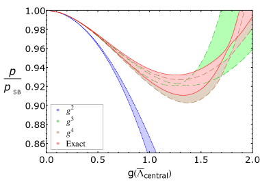
Figure 1: The Nf=3subscript𝑁f3N_{\mbox{\scriptsize f}}=3 zero density normalized pressure plotted as a function of the coupling g(Λ¯central)𝑔subscript¯Λcentralg(\bar{\Lambda}_{\rm central}), evaluated to one-loop order in HTLpt and truncated at orders g2superscript𝑔2g^{2} (blue, dotted lines), g3superscript𝑔3g^{3} (green, dot-dashed), g4superscript𝑔4g^{4} (brown, dashed), and not at all (red, solid).

In the m/T𝑚𝑇m/T- expansion, the one-loop expressions for the pressure as well as the second and fourth-order QNS were first obtained in ref. sylvain1 . These purely analytical results read

pHTLptHigh-T(T,𝝁)superscriptsubscript𝑝HTLptHigh-T𝑇𝝁\displaystyle p_{\mbox{\scriptsize HTLpt}}^{\mbox{\scriptsize\tiny High-T}}\left(T,\bm{\mu}\right) =\displaystyle= dAπ2T445{1+NcdAf(74+30μ^f2+60μ^f4)152m^D2\displaystyle\frac{d_{\mbox{\scriptsize A}}\pi^{2}T^{4}}{45}\Bigg{\{}1+\frac{N_{\mbox{\scriptsize c}}}{d_{\mbox{\scriptsize A}}}\sum_{f}\bigg{(}\frac{7}{4}+30\ \hat{\mu}_{f}^{2}+60\ \hat{\mu}_{f}^{4}\bigg{)}-\frac{15}{2}\hat{m}_{\mbox{\scriptsize D}}^{2}\, (27)
30NcdAf(1+12μ^f2)m^qf2+30m^D330subscript𝑁csubscript𝑑Asubscript𝑓112superscriptsubscript^𝜇𝑓2superscriptsubscript^𝑚qf230superscriptsubscript^𝑚D3\displaystyle\ \ \ \ \ \ \ \ \ \ \ \ -\frac{30\ N_{\mbox{\scriptsize c}}}{d_{\mbox{\scriptsize A}}}\sum_{f}\bigg{(}1+12\ \hat{\mu}_{f}^{2}\bigg{)}\hat{m}_{\mbox{\scriptsize q${}_{f}$}}^{2}+30\ \hat{m}_{\mbox{\scriptsize D}}^{3}\,
+454(γE72+π23+logΛ¯4πT)m^D4454subscript𝛾E72superscript𝜋23¯Λ4𝜋𝑇superscriptsubscript^𝑚D4\displaystyle\ \ \ \ \ \ \ \ \ \ \ \ +\frac{45}{4}\bigg{(}\gamma_{\mbox{\scriptsize\tiny E}}-\frac{7}{2}+\frac{\pi^{2}}{3}+\log\frac{\bar{\Lambda}}{4\,\pi\,T}\bigg{)}\ \hat{m}_{\mbox{\scriptsize D}}^{4}\,
+60NcdA(6π2)fm^qf4+𝒪(m^D6,m^qf6)},\displaystyle\ \ \ \ \ \ \ \ \ \ \ \ +\frac{60\ N_{\mbox{\scriptsize c}}}{d_{\mbox{\scriptsize A}}}\bigg{(}6-\pi^{2}\bigg{)}\sum_{f}\hat{m}_{\mbox{\scriptsize q${}_{f}$}}^{4}+{\cal O}\left(\hat{m}_{\mbox{\scriptsize D}}^{6},\hat{m}_{\mbox{\scriptsize q${}_{f}$}}^{6}\right)\Bigg{\}}\,,
χu2χu2,SBsubscript𝜒u2subscript𝜒u2SB\displaystyle\frac{\chi_{\rm u2}}{\chi_{\rm u2,SB}} =\displaystyle= 13dA8Ncπ2g2+dA(1+Nf2Nc)1/23/Nc8π3g3+dA32π4(1+Nf2Nc)13subscript𝑑A8subscript𝑁csuperscript𝜋2superscript𝑔2subscript𝑑Asuperscript1subscript𝑁f2subscript𝑁c123subscript𝑁c8superscript𝜋3superscript𝑔3subscript𝑑A32superscript𝜋41subscript𝑁f2subscript𝑁c\displaystyle 1-\frac{3\,d_{\mbox{\scriptsize A}}}{8\,N_{\mbox{\scriptsize c}}\,\pi^{2}}\,\,g^{2}+d_{\mbox{\scriptsize A}}\left(1+\frac{N_{\mbox{\scriptsize f}}}{2\,N_{\mbox{\scriptsize c}}}\right)^{1/2}\frac{\sqrt{3/N_{\mbox{\scriptsize c}}}}{8\,\pi^{3}}\,\,\,g^{3}+\frac{d_{\mbox{\scriptsize A}}}{32\,\pi^{4}}\left(1+\frac{N_{\mbox{\scriptsize f}}}{2\,N_{\mbox{\scriptsize c}}}\right) (28)
×[π2372+γE+logΛ¯4πT+dA(6π2)4Nc(2Nc+Nf)]g4+𝒪(g6),absentdelimited-[]superscript𝜋2372subscript𝛾E¯Λ4𝜋𝑇subscript𝑑A6superscript𝜋24subscript𝑁c2subscript𝑁csubscript𝑁fsuperscript𝑔4𝒪superscript𝑔6\displaystyle\ \times\Bigg{[}\frac{\pi^{2}}{3}-\frac{7}{2}+\gamma_{\mbox{\scriptsize\tiny E}}+\log\frac{\bar{\Lambda}}{4\,\pi\,T}+\frac{d_{\mbox{\scriptsize A}}\,\left(6-\pi^{2}\right)}{4\,N_{\mbox{\scriptsize c}}\,\left(2\,N_{\mbox{\scriptsize c}}+N_{\mbox{\scriptsize f}}\right)}\,\Bigg{]}\,g^{4}+{\cal O}(g^{6})\,,
χu4χu4,SBsubscript𝜒u4subscript𝜒u4SB\displaystyle\frac{\chi_{\rm u4}}{\chi_{\rm u4,SB}} =\displaystyle= 13dA8Ncπ2g2+3dANfNc(1+Nf2Nc)1/23/Nc32π3g3+3dA32π413subscript𝑑A8subscript𝑁csuperscript𝜋2superscript𝑔23subscript𝑑Asubscript𝑁fsubscript𝑁csuperscript1subscript𝑁f2subscript𝑁c123subscript𝑁c32superscript𝜋3superscript𝑔33subscript𝑑A32superscript𝜋4\displaystyle 1-\frac{3\,d_{\mbox{\scriptsize A}}}{8\,N_{\mbox{\scriptsize c}}\,\pi^{2}}\,\,g^{2}+3\,d_{\mbox{\scriptsize A}}\,\frac{N_{\mbox{\scriptsize f}}}{N_{\mbox{\scriptsize c}}}\left(1+\frac{N_{\mbox{\scriptsize f}}}{2\,N_{\mbox{\scriptsize c}}}\right)^{-1/2}\frac{\sqrt{3/\,N_{\mbox{\scriptsize c}}}}{32\,\pi^{3}}\,\,g^{3}+\frac{3\,d_{\mbox{\scriptsize A}}}{32\,\pi^{4}} (29)
×(Nf2Nc)[π2372+γE+logΛ¯4πT+dA(6π2)12NcNf]g4+𝒪(g6),absentsubscript𝑁f2subscript𝑁cdelimited-[]superscript𝜋2372subscript𝛾E¯Λ4𝜋𝑇subscript𝑑A6superscript𝜋212subscript𝑁csubscript𝑁fsuperscript𝑔4𝒪superscript𝑔6\displaystyle\ \times\left(\frac{N_{\mbox{\scriptsize f}}}{2\,N_{\mbox{\scriptsize c}}}\right)\Bigg{[}\frac{\pi^{2}}{3}-\frac{7}{2}+\gamma_{\mbox{\scriptsize\tiny E}}+\log\frac{\bar{\Lambda}}{4\,\pi\,T}+\frac{d_{\mbox{\scriptsize A}}\,\left(6-\pi^{2}\right)}{12\,N_{\mbox{\scriptsize c}}\,N_{\mbox{\scriptsize f}}}\,\Bigg{]}\,g^{4}+{\cal O}(g^{6})\,,\ \ \ \ \ \ \ \

the detailed derivation of which we present in appendix E. The mass parameters mDsubscript𝑚Dm_{\mbox{\scriptsize D}} and mqfsubscript𝑚qfm_{\mbox{\scriptsize q${}_{f}$}} are again given by eq. (6).

3.2 Convergence of the m/T𝑚𝑇m/T- expansion

To study the convergence of the mass expansion, we specialize to the Nf=3subscript𝑁f3N_{\mbox{\scriptsize f}}=3 case and inspect the μf=0subscript𝜇𝑓0\mu_{f}=0 pressure as a function of g(Λ¯central)𝑔subscript¯Λcentralg(\bar{\Lambda}_{\rm central}), normalized to the corresponding noninteracting Stefan-Boltzmann result. We note that Λ¯centralsubscript¯Λcentral\bar{\Lambda}_{\rm central} corresponds to the central renormalization scale, as defined in section (4.1). The different bands shown in figure 1 correspond to truncations at different orders in m/Tgsimilar-to𝑚𝑇𝑔m/T\sim g, and are generated by varying the renormalization scale Λ¯¯Λ\bar{\Lambda} by a factor of two around its central value. We see from here that with the exception of the most naive truncation at order g2superscript𝑔2g^{2}, the truncated results are not only in good agreement with each other, but even with the exact untruncated band. For values of g𝑔g relevant for our calculation, the differences between the various bands are of the order of one per cent, which can be considered an extremely positive outcome. Note also that for values of g𝑔g below 1.5, the widths of the bands somewhat surprisingly become larger as we go to higher orders in the m/T𝑚𝑇m/T- expansion.

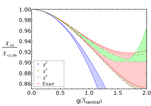
Finally, in figure 2 we perform a similar analysis of the second (left) and fourth (right) order QNS, also normalized to their Stefan-Boltzmann limits. We again see that the g3superscript𝑔3g^{3} and g4superscript𝑔4g^{4} bands are in good agreement with each other as well as with the exact results. We also observe that the agreement between the g4superscript𝑔4g^{4} results and the exact ones are especially good and much faster than for the μf=0subscript𝜇𝑓0\mu_{f}=0 pressure; in particular for the fourth-order QNS, the g4superscript𝑔4g^{4} truncation is seen to almost coincide with the exact band. This excellent convergence of the m/T𝑚𝑇m/T- expansion is in agreement with observations made for the three-loop scalar ϕ4superscriptitalic-ϕ4\phi^{4} theory in ref. motspt . Although it was noted in this work that the convergence slightly worsens as one proceeds to higher loop orders, this gives us some confidence that the m/T𝑚𝑇m/T-expansion is in general a good approximation in HTLpt calculations.
Refer to caption
Refer to caption
Figure 2: The properly normalized Nf=3subscript𝑁f3N_{\mbox{\scriptsize f}}=3 second (left) and fourth (right) order QNS plotted as functions of the coupling g(Λ¯central)𝑔subscript¯Λcentralg(\bar{\Lambda}_{\rm central}) within one-loop HTLpt. The results are also truncated at orders g2superscript𝑔2g^{2} (blue, dotted lines), g3superscript𝑔3g^{3} (green, dot-dashed), g4superscript𝑔4g^{4} (brown, dashed), and not at all (red, solid).

4 Results and comparison with lattice data

In this section, we present our results for the μf0subscript𝜇𝑓0\mu_{f}\neq 0 pressure as well as the associated quark number susceptibilities obtained both from our exact one-loop HTLpt calculation as well as the DR motivated resummation introduced in section 2.2. We then compare these results with state-of-the-art lattice data wuppertalcharge ; bieleHighT ; biele1 ; biele2 ; Borsanyi_delta_P ; handsu6u2 ; gupta as well as a very recent three-loop HTLpt calculation haque . We begin by explaining how various parameters in the DR and HTLpt results are fixed, and then move on to consider first the three- and later the two-flavor case.

4.1 Fixing the parameters

In perturbative calculations at high temperature and zero quark chemical potentials, the renormalization scale Λ¯¯Λ\bar{\Lambda} is typically chosen to be of order Λ¯2πT¯Λ2𝜋𝑇\bar{\Lambda}\approx 2\pi T, dictated by the thermal mass of the lowest nonvanishing (bosonic) Matsubara mode. With high order perturbative results available for a number of quantities, different refinements of this choice are however also possible, based on schemes such as the Fastest Apparent Convergence (FAC) or the Principle of Minimal Sensitivity (PMS). As is customary in recent literature (see e.g. kajantie4 ), we apply in all of our results the FAC scheme to the NLO gauge coupling of EQCD, providing the values Λ¯central=1.445×2πTsubscript¯Λcentral1.4452𝜋𝑇\bar{\Lambda}_{\rm central}=1.445\times 2\pi T for three quark flavors as well as Λ¯central=1.291×2πTsubscript¯Λcentral1.2912𝜋𝑇\bar{\Lambda}_{\rm central}=1.291\times 2\pi T for two flavors.

The most straightforward way to generalize the above setup to nonzero density is to perform the exact same procedure, i.e. solve Λ¯¯Λ\bar{\Lambda} from the equation αE7=0subscript𝛼E70\alpha_{\mbox{\scriptsize E7}}=0, at nonvanishing μfsubscript𝜇𝑓\mu_{f}. This leads to the results

Λ¯centralNf=3superscriptsubscript¯ΛcentralsubscriptNf3\displaystyle\bar{\Lambda}_{\rm central}^{\rm N_{\mbox{\scriptsize f}}=3} =\displaystyle= 0.9344×2πTexp(127f[Ψ(12+iμ^f)+Ψ(12iμ^f)]),0.93442𝜋𝑇127subscript𝑓delimited-[]Ψ12𝑖subscript^𝜇𝑓Ψ12𝑖subscript^𝜇𝑓\displaystyle\frac{0.9344\times 2\pi T}{\exp\left(\frac{1}{27}\sum_{f}\left[\Psi(\frac{1}{2}+i\hat{\mu}_{f})+\Psi(\frac{1}{2}-i\hat{\mu}_{f})\right]\right)}\,, (30)
Λ¯centralNf=2superscriptsubscript¯ΛcentralsubscriptNf2\displaystyle\bar{\Lambda}_{\rm central}^{\rm N_{\mbox{\scriptsize f}}=2} =\displaystyle= 0.9847×2πTexp(129f[Ψ(12+iμ^f)+Ψ(12iμ^f)]),0.98472𝜋𝑇129subscript𝑓delimited-[]Ψ12𝑖subscript^𝜇𝑓Ψ12𝑖subscript^𝜇𝑓\displaystyle\frac{0.9847\times 2\pi T}{\exp\left(\frac{1}{29}\sum_{f}\left[\Psi(\frac{1}{2}+i\hat{\mu}_{f})+\Psi(\frac{1}{2}-i\hat{\mu}_{f})\right]\right)}\,, (31)

where ΨΨ\Psi denotes the digamma function. To assess the sensitivity of our results to the choice of the renormalization scale, we will in addition always vary Λ¯¯Λ\bar{\Lambda} by a factor of two around these central values.

With the running gauge coupling g𝑔g, we follow the standard procedure of working with a two-loop expression in the DR case and a one-loop coupling in LO HTLpt. To determine the value of ΛMS¯subscriptΛ¯MS\Lambda_{\rm\overline{MS}}, we on the other hand take the recent lattice result αs(1.5GeV)=0.326subscript𝛼s1.5GeV0.326\alpha_{\mbox{\scriptsize s}}(1.5\;{\rm GeV})=0.326 runningalpha , and demand that our running coupling agrees with it for Λ¯central=1.5subscript¯Λcentral1.5\bar{\Lambda}_{\rm central}=1.5 GeV. For Nf=3subscript𝑁f3N_{\mbox{\scriptsize f}}=3, this yields the values ΛMS¯=176subscriptΛ¯MS176\Lambda_{\rm\overline{MS}}=176 MeV and 283 MeV for the one- and two-loop couplings, while for Nf=2subscript𝑁f2N_{\mbox{\scriptsize f}}=2, the corresponding results read ΛMS¯=204subscriptΛ¯MS204\Lambda_{\rm\overline{MS}}=204 MeV and 324 MeV. These parameters are also varied by 30 MeV around the central values quoted here.

In the recent three-loop HTLpt results of haque , to which we will compare our calculations below, the authors used two separate renormalization scales ΛgsubscriptΛg\Lambda_{\mbox{\scriptsize g}} and ΛqsubscriptΛq\Lambda_{\mbox{\scriptsize q}} for purely gluonic and fermionic graphs, respectively. They took the central values Λg=2πTsubscriptΛg2𝜋𝑇\Lambda_{\mbox{\scriptsize g}}=2\pi T and Λq=2πT2+μ2/π2subscriptΛq2𝜋superscript𝑇2superscript𝜇2superscript𝜋2\Lambda_{\mbox{\scriptsize q}}=2\pi\sqrt{T^{2}+\mu^{2}/\pi^{2}} and varied both scales by a factor of two in order to estimate the renormalization scale sensitivity of their results. For the gauge coupling, they used a one-loop running with ΛMS¯=176subscriptΛ¯MS176\Lambda_{\rm\overline{MS}}=176 MeV, which for Nf=3subscript𝑁f3N_{\mbox{\scriptsize f}}=3 gives αs(1.5GeV)=0.326subscript𝛼s1.5GeV0.326\alpha_{\mbox{\scriptsize s}}(1.5\;{\rm GeV})=0.326 as well.

4.2 Results for three flavors

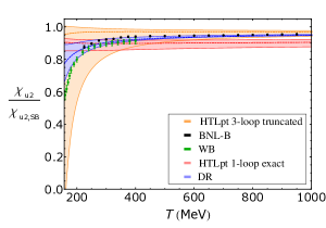
Let us begin the analysis of our results from the quark number susceptibilities in the physically most interesting case of Nf=3subscript𝑁f3N_{\mbox{\scriptsize f}}=3. In figure 3 (left), we display the second order diagonal susceptibility χu2subscript𝜒u2\chi_{\rm u2} normalized to its Stefan-Boltzmann limit χu2,SB=T2subscript𝜒u2SBsuperscript𝑇2\chi_{\rm u2,SB}=T^{2}. The blue band in the figure corresponds to the DR result, obtained by varying the values of both Λ¯¯Λ\bar{\Lambda} and ΛMS¯subscriptΛ¯MS\Lambda_{\rm\overline{MS}} in the ranges explained above, while the red and orange bands are the exact one-loop and truncated three-loop HTLpt results. The thick dashed lines inside the bands correspond to the central values of the renormalization and QCD scales. Finally, we note that the three-loop HTLpt band in fact corresponds to the baryon (and not quark) number susceptibility haque ; however, for the second order susceptibilities the difference between these two quantities should be hardly visible bieleHighT .
Refer to caption

​​​Refer to caption

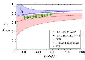
Figure 3: The Nf=3subscript𝑁f3N_{\mbox{\scriptsize f}}=3 second (left) and fourth (right) order diagonal QNS normalized to their respective Stefan-Boltzmann values. The truncated three-loop HTLpt results are from haque and the lattice data are from BNL-Bielefeld (BNL-B) bieleHighT ; biele1 ; biele2 and Wuppertal-Budapest (WB) wuppertalcharge ; chi4 .

The widths of the bands shown indicate that the scale dependence of the DR result is extremely weak, except for the very lowest temperatures. At the same time, the one- and three-loop HTLpt results are also quite close to one another for temperatures above 500 MeV, indicating that the quantity under consideration nicely converges at these temperatures.444Although we do not show it in figure 3 (left), the two-loop HTLpt result for the second-order susceptibility is also quite close to the three-loop HTLpt result for temperatures above 500 MeV mikehaque . In figure 3 (left) we also display lattice results from both the BNL-Bielefeld (BNL-B, black dots) bieleHighT and Wuppertal-Budapest (WB, green dots) wuppertalcharge collaborations. Both sets of data have been continuum extrapolated. We observe that the DR and three-loop HTLpt results are all in good agreement with the two lattice results for temperatures of roughly 500 MeV and higher; at even lower T𝑇T, some differences do, however, occur and it is the resummed DR result that seems to agree better with the lattice data points.
Refer to caption
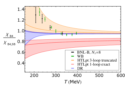
Figure 4: The Nf=3subscript𝑁f3N_{\mbox{\scriptsize f}}=3 fourth order diagonal baryon number susceptibility normalized to its Stefan-Boltzmann value. The truncated three-loop HTLpt results are from haque , and the lattice data from Wuppertal-Budapest (WB) chi4 and BNL-Bielefeld (BNL-B) Bazavov13 .

In figure 3 (right), we next show our results for the fourth order diagonal QNS χu4subscript𝜒u4\chi_{\rm u4} normalized to the corresponding Stefan-Boltzmann limit χu4,SB=6/π2subscript𝜒u4SB6superscript𝜋2\chi_{\rm u4,SB}=6/\pi^{2}. Once again, the thick dashed line in each band corresponds to the central value of the renormalization and QCD scales, while the width of the band indicates the sensitivity of the corresponding result with respect to these parameters. The continuum extrapolated WB lattice data are this time taken from ref. chi4 , while the HISQ Nτ=8subscript𝑁𝜏8N_{\tau}=8 BNL-B results are from refs. biele1 ; biele2 . Our resummed DR and exact one-loop HTLpt results appear to reproduce the qualitative trend of the lattice results for most temperatures, but this time there is a more sizable difference between these two theoretical predictions over the entire temperature range. While for the lowest temperatures the lattice data seem to favor our one-loop HTLpt result, the difference between the lattice points and the DR result is seen to decrease with increasing temperature. It will thus be very interesting to see, how future high-precision lattice data at T=500𝑇500T=500 MeV and higher will affect these conclusions.

Note that figure 3 (right) lacks a band corresponding to the three-loop HTLpt calculation of haque . This is due to the fact that, as pointed out above, at present the three-loop HTLpt results are only available for baryon number susceptibilities, which differ from the quark number ones by off-diagonal contributions, estimated to be non-negligible in this case bieleHighT . To this end, in figure 4 we compare our results for the fourth order baryon number susceptibility χB4subscript𝜒B4\chi_{\mbox{\scriptsize B4}} normalized to the corresponding Stefan-Boltzmann limit χB4,SB=2/(9π2)subscript𝜒B4SB29superscript𝜋2\chi_{\rm B4,SB}=2/(9\pi^{2}), obtained using the resummed DR approach as well as exact one-loop HTLpt, to the three-loop HTLpt result of ref. haque and lattice data from both the Wuppertal-Budapest (WB) chi4 and BNL-Bielefeld (BNL-B) Bazavov13 collaborations. Our notations for the bands and the dashed curves therein are defined as before.
Refer to caption
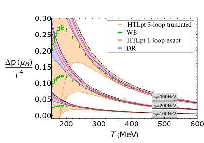
Figure 5: The difference between the Nf=3subscript𝑁f3N_{\mbox{\scriptsize f}}=3 pressure evaluated at nonvanishing chemical potentials and at μf=0subscript𝜇𝑓0\mu_{f}=0. The dashed lines indicate the respective Stefan-Boltzmann limits. The three-loop HTLpt results are again from haque , and the lattice data from Wuppertal-Budapest (WB) Borsanyi_delta_P .

From the figure, we see that the central lines from the resummed DR and three-loop HTLpt results for χB4subscript𝜒B4\chi_{\rm B4} are in good agreement in the entire temperature range shown, and moreover overlap with the lattice data from 350 MeV onwards. The resummed DR result, however, has a smaller band than the three-loop HTLpt result. We also note that the convergence of the successive HTLpt loop approximations for the fourth-order susceptibility is not as good as the convergence found for the second-order susceptibility. This seems to be due to the fact that the fourth-order susceptibility is more sensitive to over-counting which occurs in low loop-order HTLpt. At three-loop order, this over-counting is fixed through order g5superscript𝑔5g^{5}, if the result is perturbatively expanded.

Inspecting next the equation of state itself, in figure 5 we show the difference of the pressure evaluated with nonzero and vanishing quark chemical potentials, which are chosen to be the same for each flavor with μB=100subscript𝜇B100\mu_{\mbox{\scriptsize B}}=100, 200, and 300 MeV. The ‘continuum estimated’ lattice data quoted in this figure are from Borsanyi_delta_P , and are based on an expansion of the pressure up to and including 𝒪(μf2)𝒪superscriptsubscript𝜇𝑓2{\cal O}(\mu_{f}^{2}). The HTLpt and DR results are on the other hand accurate to all orders in μfsubscript𝜇𝑓\mu_{f}, being only restricted by assumptions inherent in the HTLpt and DR resummation schemes; in the latter case, the results have been shown to be valid for all T𝑇T and μfsubscript𝜇𝑓\mu_{f} satisfying πTgμfgreater-than-or-equivalent-to𝜋𝑇𝑔subscript𝜇𝑓\pi T\gtrsim g\mu_{f} ipp3 , which clearly is the case here. As expected based on the earlier analysis of aleksi3 , we observe a good agreement between our results and the lattice data down to temperatures of the order of 250 MeV. Also, it is important to note that both the DR and LO HTLpt results are clearly distinct from the corresponding Stefan-Boltzmann limits, indicated by the dashed black lines in the figure.

4.3 Results for two flavors

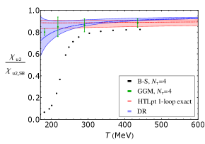
Moving on to the two flavor case, widely studied with lattice methods, we first examine the behavior of the second-order diagonal QNS normalized to its Stefan-Boltzmann limit, displayed in figure 6 (left). As can be seen from here, both of our perturbative bands are now somewhat wider (and reside lower) than in the three flavor case, but their general trends are very similar.555Note that at the moment three-loop HTLpt results are not yet available in the case of two quark flavors. Also shown in this figure are lattice results from the Bielefeld-Swansea collaboration (B-S, black dots) handsu6u2 as well as those by Gavai, Gupta and Majumdar (GGM, green dots) gupta , both of which were computed on Nτ=4subscript𝑁𝜏4N_{\tau}=4 lattices. One issue in transfering the lattice results to physical units is the determination of the critical temperature appropriate for the lattice spacings used. For the results of gupta , the problem is easily resolved, as we may simply use the value Tc=145subscript𝑇c145T_{\mbox{\scriptsize c}}=145 MeV, quoted as the pseudo-critical temperature in the same reference. In the case of the B-S results, obtained using p4-improved staggered fermions, more care must, however, be exercised; here, we have chosen to follow the approach of Peikert ; Peikert2 , which leads to the value Tc=223subscript𝑇c223T_{\mbox{\scriptsize c}}=223 MeV. As neither of these values correspond to the correct pseudo-critical temperature (in the chiral limit, Tc=173subscript𝑇c173T_{\mbox{\scriptsize c}}=173 MeV AbsoluteScale ), and they moreover deviate from it in opposite directions, we urge the reader to take the lattice data points quoted in the figure with some reservation.
Refer to caption

​​​​Refer to caption

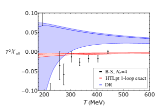
Figure 6: The second-order diagonal QNS normalized to its Stefan-Boltzmann value (left), and the sixth-order diagonal QNS multiplied by T2superscript𝑇2T^{2} (right), both evaluated for Nf=2subscript𝑁f2N_{\mbox{\scriptsize f}}=2. The lattice data sets have been taken from Bielefeld-Swansea (B-S) handsu6u2 as well as from gupta (GGM). Note that both data sets in the left figure in fact do include error bars, even though for the B-S data they are hardly visible.

From figure 6 (left), we see that the agreement between our HTLpt and DR bands is very good over the entire range of temperatures displayed. However, unlike in the three flavor case, the agreement between the perturbative bands and the lattice data of handsu6u2 is clearly not optimal. We suspect that this may well be related to the discrepancy between the results of the two different lattice groups, which itself can be traced back to the difference between the values of Tcsubscript𝑇cT_{\mbox{\scriptsize c}} used in converting the lattice data to physical units. Naively, the perturbative results seem to be in better agreement with gupta , but in the absence of continuum extrapolated lattice results, firm conclusions are difficult to draw.
Refer to caption
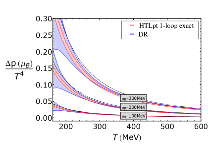
Figure 7: The difference between the pressure evaluated at finite and vanishing chemical potentials, for Nf=2subscript𝑁f2N_{\mbox{\scriptsize f}}=2. The dashed lines denote the Stefan-Boltzmann limits in the three cases considered.

Next, consider the sixth order diagonal QNS χu6subscript𝜒u6\chi_{\rm u6}, which we display in figure 6 (right) together with lattice data again from Bielefeld-Swansea (B-S) handsu6u2 . As we now encounter the first case, where the weak coupling expansion only begins at order g3superscript𝑔3g^{3}, it is not surprising that our exact one-loop HTLpt and DR results are seen to disagree: While the DR band is above zero for most of the relevant temperatures, the one-loop HTLpt result is consistently negative. As noted above, at the moment there are unfortunately no published three-loop HTLpt results available for this quantity; given the good agreement of our resummed DR results with the three-loop HTLpt ones for all other susceptibilities, we however suspect that this will be the case also for the sixth order QNS. This despite the fact that according to figure 6 (right) the non-continuum extrapolated lattice data of handsu6u2 appear to favor our exact one-loop HTLpt results over the DR ones at least at low temperatures.

Finally, in addition to the susceptibilities, we can inspect the behavior of the pressure at nonzero chemical potentials, also for the case of Nf=2subscript𝑁f2N_{\mbox{\scriptsize f}}=2. This is done in figure 7, where in the absence of lattice and three-loop HTLpt results we only display two perturbative bands corresponding to our one-loop HTLpt and four-loop DR calculations. Not surprisingly, the HTLpt and DR results are again in good agreement with each other, though the DR bands widen at low temperatures in a more pronounced way than in the three flavor case. Finally, we notice that both sets of bands again differ from their Stefan-Boltzmann limits in a noticeable way.

5 Conclusions and outlook

In this paper, we have computed the pressure of deconfined quark-gluon plasma at high temperature and nonzero quark number density using two variations of resummed perturbation theory. First, we employed hard-thermal-loop perturbation theory (HTLpt) to derive an exact one-loop result, after which we performed a resummation inspired by dimensional reduction (DR) to its existing unresummed four-loop weak coupling expansion. The computation within HTLpt also included some new technical improvements, as we were able to implement the renormalization procedure of HTLpt in a significantly more straightforward and elegant manner than was done in the original works of Jens2 ; Jens3 , as well as to refine the calculation of a couple of the renormalization constants originally obtained in these references. Finally, we also studied the convergence of the m/T𝑚𝑇m/T-expansion within one-loop HTLpt, observing that the truncated results rapidly converge towards the exact unexpanded ones. This gives us confidence in higher-order calculations within HTLpt mikehaque ; Haque1 ; haque , where the m/T𝑚𝑇m/T-expansion has been used.

After obtaining the pressure as a function of temperature and quark chemical potentials, we derived predictions for the second, fourth and sixth order diagonal quark number susceptibilities (QNS) as well as for the chemical potential dependence of the pressure itself. Agreement between the HTLpt and resummed DR results, as well as between them and lattice data, was consistently observed to be good starting at temperatures below 500 MeV with the sole exception of the sixth order QNS, which we studied for two quark flavors. For this quantity, the weak coupling expansion of which starts only at order g3superscript𝑔3g^{3}, the one-loop HTLpt and resummed DR predictions were seen to be in clear disagreement. At the moment, no continuum extrapolated lattice data exist for this observable, but the available Nτ=4subscript𝑁𝜏4N_{\tau}=4 data of the Bielefeld-Swansea collaboration handsu6u2 appear to favor the one-loop HTLpt prediction for most temperatures. However, given the good agreement between our DR resummation and three-loop HTLpt for the other susceptibilities, we have reasons to believe that the forthcoming three-loop HTLpt htlptforth and our present DR results will be in agreement for this quantity as well.

In summary, our results can be taken as an indication that for temperatures above 250-500 MeV (somewhat dependent on the quantity under study), the behavior of quark number susceptibilities and the chemical potential dependence of the pressure can be accurately described via resummed perturbation theory. This is an important observation for two separate reasons. First, it indicates that at least the fermionic sector of QCD appears to allow a description in terms of weakly interacting quasiparticles not only at asymptotically high energy density, but already in a regime that can be reached in modern colliders. Secondly and perhaps even more importantly, one should recall that the methods employed in our calculation work well even at very large values of the ratio μf/Tsubscript𝜇𝑓𝑇\mu_{f}/T, implying that our results extend to a region of the QCD phase diagram, where no other first principles method is available. We are indeed hopeful that the perturbative results discussed in this paper — in particular those based on our DR resummation and the recent three-loop HTLpt calculation of haque — will turn out to be of practical phenomenological use in the eventual analysis of heavy ion data from the FAIR facility of GSI, whose goal is to probe the finite-density regime of the QCD phase diagram.

Acknowledgements.
We are grateful to Szabolcs Borsányi, Gergely Endrődi, Pietro Giudice, Simon Hands, Najmul Haque, Frithjof Karsch, Igor Kondrashuk, Edwin Laermann, Mikko Laine, Munshi Mustafa, Péter Petreczky, Anton Rebhan, Kari Rummukainen, Christian Schmidt, Sayantan Sharma, and Mathias Wagner for useful discussions. We would also like to thank Szabolcs Borsányi and Frithjof Karsch for providing us with their latest lattice data. S.M. and A.V. were supported by the Sofja Kovalevskaja program and N.S. by the Postdoctoral Research Fellowship of the Alexander von Humboldt Foundation. M.S. was supported in part by the DOE Grant No. DE-SC0004104.

Appendix A Notation

In the imaginary time formalism of thermal field theory, the four-momentum K=(K0,𝐤)𝐾subscript𝐾0𝐤K=(K_{0},{\bf k}) is Euclidean, K2=K02+𝐤2superscript𝐾2superscriptsubscript𝐾02superscript𝐤2K^{2}=K_{0}^{2}+{\bf k}^{2}. The norm of the spatial component of this momentum is denoted by k|𝐤|𝑘𝐤k\equiv\left|{\bf k}\right|, while its temporal component is discrete,

K0subscript𝐾0\displaystyle K_{0} =\displaystyle= ωn,(bosons),subscript𝜔𝑛bosons\displaystyle\omega_{n}\;,\hskip 56.9055pt({\rm bosons})\;, (32)
K0subscript𝐾0\displaystyle K_{0} =\displaystyle= ω~niμf,(fermions),subscript~𝜔𝑛𝑖subscript𝜇𝑓fermions\displaystyle\tilde{\omega}_{n}-i\mu_{f}\;,\hskip 28.45274pt({\rm fermions})\;, (33)

where ωn=2nπTsubscript𝜔𝑛2𝑛𝜋𝑇\omega_{n}=2n\pi T and ω~n=(2n+1)πTsubscript~𝜔𝑛2𝑛1𝜋𝑇\tilde{\omega}_{n}=(2n+1)\pi T, with n𝑛n an integer. Here μfsubscript𝜇𝑓\mu_{f} is the quark chemical potential of the flavor f𝑓f. We define the dimensionally regularized sum-integrals by

Ksubscript𝐾\displaystyle\hbox{$\sum$}\!\!\!\!\!\!\!\int_{K} =\displaystyle= (Λ¯2eγE4π)ϵTωnd32ϵ𝐤(2π)32ϵ,superscriptsuperscript¯Λ2superscript𝑒subscript𝛾E4𝜋italic-ϵ𝑇subscriptsubscript𝜔𝑛superscriptd32italic-ϵ𝐤superscript2𝜋32italic-ϵ\displaystyle\left(\frac{\bar{\Lambda}^{2}\,e^{\gamma_{\mbox{\scriptsize\tiny E}}}}{4\pi}\right)^{\epsilon}T\sum_{\omega_{n}}\int\kern-5.0pt\frac{\mathop{{\rm d}^{3-2\epsilon}\!}\nolimits{\bf k}}{(2\pi)^{3-2\epsilon}}\;, (34)
{K}subscript𝐾\displaystyle\hbox{$\sum$}\!\!\!\!\!\!\!\int_{\{K\}} =\displaystyle= (Λ¯2eγE4π)ϵTω~nd32ϵ𝐤(2π)32ϵ,superscriptsuperscript¯Λ2superscript𝑒subscript𝛾E4𝜋italic-ϵ𝑇subscriptsubscript~𝜔𝑛superscriptd32italic-ϵ𝐤superscript2𝜋32italic-ϵ\displaystyle\left(\frac{\bar{\Lambda}^{2}\,e^{\gamma_{\mbox{\scriptsize\tiny E}}}}{4\pi}\right)^{\epsilon}T\sum_{\tilde{\omega}_{n}}\int\kern-5.0pt\frac{\mathop{{\rm d}^{3-2\epsilon}\!}\nolimits{\bf k}}{(2\pi)^{3-2\epsilon}}\;, (35)

and from here onwards will abbreviate the integral over the three-momenta by

𝐤subscript𝐤\displaystyle\int_{\bf k} \displaystyle\equiv (Λ¯2eγE4π)ϵd32ϵ𝐤(2π)32ϵ.superscriptsuperscript¯Λ2superscript𝑒subscript𝛾E4𝜋italic-ϵsuperscriptd32italic-ϵ𝐤superscript2𝜋32italic-ϵ\displaystyle\left(\frac{\bar{\Lambda}^{2}\,e^{\gamma_{\mbox{\scriptsize\tiny E}}}}{4\pi}\right)^{\epsilon}\int\kern-5.0pt\frac{\mathop{{\rm d}^{3-2\epsilon}\!}\nolimits{\bf k}}{(2\pi)^{3-2\epsilon}}\;. (36)

Throughout our work, we use the modified minimal subtraction scheme MS¯¯MS{\overline{\mbox{{\mbox{\scriptsize MS}}}}} of dimensional regularization in d=32ϵ𝑑32italic-ϵd=3-2\epsilon dimensions, where the renormalization scale Λ¯¯Λ\bar{\Lambda} is related to the minimal subtraction (MS) one via Λ¯24πΛ2exp(γE)superscript¯Λ24𝜋superscriptΛ2subscript𝛾E\bar{\Lambda}^{2}\equiv 4\pi\Lambda^{2}\exp\left(-\gamma_{\mbox{\scriptsize\tiny E}}\right), with γE0.577216subscript𝛾E0.577216\gamma_{\mbox{\scriptsize\tiny E}}\approx 0.577216 the Euler-Mascheroni constant. Finally, the dimensionalities of the fermion and gluon representations of the SU(Ncsubscript𝑁cN_{\mbox{\scriptsize c}}) group are denoted by dF=NcNfsubscript𝑑Fsubscript𝑁csubscript𝑁fd_{\mbox{\scriptsize F}}=N_{\mbox{\scriptsize c}}N_{\mbox{\scriptsize f}} and dA=Nc21subscript𝑑Asuperscriptsubscript𝑁c21d_{\mbox{\scriptsize A}}=N_{\mbox{\scriptsize c}}^{2}-1, while some further group theory constants, needed in appendix B, read CA=Ncsubscript𝐶Asubscript𝑁cC_{\mbox{\scriptsize A}}=N_{\mbox{\scriptsize c}}, CF=dA/(2Nc)subscript𝐶Fsubscript𝑑A2subscript𝑁cC_{\mbox{\scriptsize F}}=d_{\mbox{\scriptsize A}}/(2N_{\mbox{\scriptsize c}}) as well as TF=Nf/2subscript𝑇Fsubscript𝑁f2T_{\mbox{\scriptsize F}}=N_{\mbox{\scriptsize f}}/2.

Appendix B Matching coefficients of EQCD

The matching constants of EQCD, defined in section 2.2, all have analytical expressions as functions of the ratios μ^fμf/(2πT)subscript^𝜇𝑓subscript𝜇𝑓2𝜋𝑇\hat{\mu}_{f}\equiv\mu_{f}/(2\pi T), derived in ref. aleksi1 . They are expressed in terms of derivatives of the generalized Riemann Zeta function, ζ(n,z)nζ(n,z)superscript𝜁𝑛𝑧subscript𝑛𝜁𝑛𝑧\zeta^{\prime}(n,z)\equiv\partial_{n}\zeta(n,z) and the digamma function Ψ(z)=Γ(z)/Γ(z)Ψ𝑧superscriptΓ𝑧Γ𝑧\Psi(z)=\Gamma^{\prime}(z)/\Gamma(z), appearing in the combinations

(n,μ1,μ2)𝑛subscript𝜇1subscript𝜇2\displaystyle\aleph(n,\mu_{1},\mu_{2}) \displaystyle\equiv (n,μ1+μ2),𝑛subscript𝜇1subscript𝜇2\displaystyle\aleph(n,\mu_{1}+\mu_{2})\,, (37)
(n,μ)𝑛𝜇\displaystyle\aleph(n,\mu) \displaystyle\equiv ζ(n,1/2iμ^)+(1)n+1ζ(n,1/2+iμ^),superscript𝜁𝑛12𝑖^𝜇superscript1𝑛1superscript𝜁𝑛12𝑖^𝜇\displaystyle\zeta^{\prime}(-n,1/2-i\ \hat{\mu})+(-1)^{n+1}\zeta^{\prime}(-n,1/2+i\ \hat{\mu})\,, (38)
(μ)𝜇\displaystyle\aleph(\mu) \displaystyle\equiv Ψ(1/2iμ^)+Ψ(1/2+iμ^),Ψ12𝑖^𝜇Ψ12𝑖^𝜇\displaystyle\Psi(1/2-i\ \hat{\mu})+\Psi(1/2+i\ \hat{\mu})\;, (39)

where n𝑛n is a non-negative integer and μ^^𝜇\hat{\mu} is real. The explicit expressions read

αE1subscript𝛼E1\displaystyle\alpha_{\mbox{\scriptsize E1}} =\displaystyle= π245Nff{dA+dF(74+30μ^f2+60μ^f4)},superscript𝜋245subscript𝑁fsubscript𝑓subscript𝑑Asubscript𝑑F7430superscriptsubscript^𝜇𝑓260superscriptsubscript^𝜇𝑓4\displaystyle\frac{\pi^{2}}{45\,N_{\mbox{\scriptsize f}}}\ \sum_{f}\bigg{\{}d_{\mbox{\scriptsize A}}+d_{\mbox{\scriptsize F}}\bigg{(}\frac{7}{4}+30\ \hat{\mu}_{f}^{2}+60\ \hat{\mu}_{f}^{4}\bigg{)}\bigg{\}}\,, (40)
αE2subscript𝛼E2\displaystyle\alpha_{\mbox{\scriptsize E2}} =\displaystyle= dA144Nff{CA+TF2(1+12μ^f2)(5+12μ^f2)},subscript𝑑A144subscript𝑁fsubscript𝑓subscript𝐶Asubscript𝑇F2112superscriptsubscript^𝜇𝑓2512superscriptsubscript^𝜇𝑓2\displaystyle-\ \frac{d_{\mbox{\scriptsize A}}}{144\,N_{\mbox{\scriptsize f}}}\ \sum_{f}\bigg{\{}C_{\mbox{\scriptsize A}}+\frac{T_{\mbox{\scriptsize F}}}{2}\bigg{(}1+12\ \hat{\mu}_{f}^{2}\bigg{)}\bigg{(}5+12\ \hat{\mu}_{f}^{2}\bigg{)}\bigg{\}}\,, (41)
αE3subscript𝛼E3\displaystyle\alpha_{\mbox{\scriptsize E3}} =\displaystyle= dA144Nff{CA2(1943logΛ¯4πT+1165+4γE383ζ(3)ζ(3)+2203ζ(1)ζ(1))\displaystyle\frac{d_{\mbox{\scriptsize A}}}{144\,N_{\mbox{\scriptsize f}}}\sum_{f}\Bigg{\{}C_{\mbox{\scriptsize A}}^{2}\bigg{(}\frac{194}{3}\log\frac{\bar{\Lambda}}{4\pi T}+\frac{116}{5}+4\gamma_{\mbox{\scriptsize\tiny E}}-\frac{38}{3}\frac{\zeta^{\prime}(-3)}{\zeta(-3)}+\frac{220}{3}\frac{\zeta^{\prime}(-1)}{\zeta(-1)}\bigg{)}\, (42)
+CATF[(1693+600μ^f2528μ^f4)logΛ¯4πT+112160+8γE\displaystyle\ \ \ \ \ \ \ \ \ \ \ +C_{\mbox{\scriptsize A}}\ T_{\mbox{\scriptsize F}}\bigg{[}\bigg{(}\frac{169}{3}+600\ \hat{\mu}_{f}^{2}-528\ \hat{\mu}_{f}^{4}\bigg{)}\log\frac{\bar{\Lambda}}{4\pi T}+\frac{1121}{60}+8\gamma_{\mbox{\scriptsize\tiny E}}\,
+2(127+48γE)μ^f2+43(11+156μ^f2)ζ(1)ζ(1)644μ^f4212748subscript𝛾Esuperscriptsubscript^𝜇𝑓24311156superscriptsubscript^𝜇𝑓2superscript𝜁1𝜁1644superscriptsubscript^𝜇𝑓4\displaystyle\ \ \ \ \ \ \ \ \ \ \ +2\,\bigg{(}127+48\gamma_{\mbox{\scriptsize\tiny E}}\bigg{)}\ \hat{\mu}_{f}^{2}+\frac{4}{3}\bigg{(}11+156\ \hat{\mu}_{f}^{2}\bigg{)}\frac{\zeta^{\prime}(-1)}{\zeta(-1)}-644\ \hat{\mu}_{f}^{4}\,
+26815ζ(3)ζ(3)+24(52(3,μf)+4iμ^f(0,μf)\displaystyle\ \ \ \ \ \ \ \ \ \ \ +\frac{268}{15}\frac{\zeta^{\prime}(-3)}{\zeta(-3)}+24\bigg{(}52\ \aleph(3,\mu_{f})+4\ i\ \hat{\mu}_{f}\ \aleph(0,\mu_{f})\,
+144iμ^f(2,μf)+(1792μ^f2)(1,μf))]\displaystyle\ \ \ \ \ \ \ \ \ \ \ +144\ i\ \hat{\mu}_{f}\ \aleph(2,\mu_{f})+\bigg{(}17-92\ \hat{\mu}_{f}^{2}\bigg{)}\ \aleph(1,\mu_{f})\bigg{)}\bigg{]}\ \ \ \ \ \ \ \ \ \ \,
+CFTF[34(1+4μ^f2)(35+332μ^f2)24(112μ^f2)ζ(1)ζ(1)\displaystyle\ \ \ \ \ \ \ \ \ \ \ +C_{\mbox{\scriptsize F}}\,T_{\mbox{\scriptsize F}}\bigg{[}\frac{3}{4}\bigg{(}1+4\ \hat{\mu}_{f}^{2}\bigg{)}\bigg{(}35+332\ \hat{\mu}_{f}^{2}\bigg{)}-24\bigg{(}1-12\ \hat{\mu}_{f}^{2}\bigg{)}\frac{\zeta^{\prime}(-1)}{\zeta(-1)}\,
144(12iμ^f(2,μf)2(1+8μ^f2)(1,μf)\displaystyle\ \ \ \ \ \ \ \ \ \ \ -144\,\bigg{(}12\ i\ \hat{\mu}_{f}\ \aleph(2,\mu_{f})-2\bigg{(}1+8\ \hat{\mu}_{f}^{2}\bigg{)}\ \aleph(1,\mu_{f})\,
iμ^f(1+4μ^f2)(0,μf))]\displaystyle\ \ \ \ \ \ \ \ \ \ \ -\ i\ \hat{\mu}_{f}\bigg{(}1+4\ \hat{\mu}_{f}^{2}\bigg{)}\ \aleph(0,\mu_{f})\bigg{)}\bigg{]}\,
+TF2[43(1+12μ^f2)(5+12μ^f2)logΛ¯4πT+13+4γE\displaystyle\ \ \ \ \ \ \ \ \ \ \ +T_{\mbox{\scriptsize F}}^{2}\bigg{[}\frac{4}{3}\bigg{(}1+12\ \hat{\mu}_{f}^{2}\bigg{)}\bigg{(}5+12\ \hat{\mu}_{f}^{2}\bigg{)}\log\frac{\bar{\Lambda}}{4\pi T}+\frac{1}{3}+4\,\gamma_{\mbox{\scriptsize\tiny E}}\,
+8(7+12γE)μ^f2+112μ^f4323(1+12μ^f2)ζ(1)ζ(1)8712subscript𝛾Esuperscriptsubscript^𝜇𝑓2112superscriptsubscript^𝜇𝑓4323112superscriptsubscript^𝜇𝑓2superscript𝜁1𝜁1\displaystyle\ \ \ \ \ \ \ \ \ \ \ +8\,\bigg{(}7+12\gamma_{\mbox{\scriptsize\tiny E}}\bigg{)}\ \hat{\mu}_{f}^{2}+112\ \hat{\mu}_{f}^{4}-\frac{32}{3}\bigg{(}1+12\ \hat{\mu}_{f}^{2}\bigg{)}\frac{\zeta^{\prime}(-1)}{\zeta(-1)}\,
6415ζ(3)ζ(3)96(8(3,μf)+12iμ^f(2,μf)\displaystyle\ \ \ \ \ \ \ \ \ \ \ -\frac{64}{15}\,\frac{\zeta^{\prime}(-3)}{\zeta(-3)}-96\bigg{(}8\ \aleph(3,\mu_{f})+12\ i\ \hat{\mu}_{f}\ \aleph(2,\mu_{f})\,
2(1+2μ^f2)(1,μf)iμ^f(0,μf))]\displaystyle\ \ \ \ \ \ \ \ \ \ \ -2\,(1+2\ \hat{\mu}_{f}^{2})\,\aleph(1,\mu_{f})-\ i\ \hat{\mu}_{f}\ \aleph(0,\mu_{f})\bigg{)}\bigg{]}\,
+288TF2Nfg{2(1+γE)μ^f2μ^g2(3,μf,μg)(3,μf,μg)\displaystyle\ \ \ \ \ \ \ \ \ \ \ +\frac{288\,T_{\mbox{\scriptsize F}}^{2}}{N_{\mbox{\scriptsize f}}}\,\sum_{g}\bigg{\{}2\ \bigg{(}1+\gamma_{\mbox{\scriptsize\tiny E}}\bigg{)}\ \hat{\mu}_{f}^{2}\ \hat{\mu}_{g}^{2}-\,\aleph(3,\mu_{f},\mu_{g})-\,\aleph(3,\mu_{f},-\mu_{g})\,
+4μ^g2(1,μf)4iμ^f((2,μf,μg)+(2,μf,μg))4superscriptsubscript^𝜇𝑔21subscript𝜇𝑓4𝑖subscript^𝜇𝑓2subscript𝜇𝑓subscript𝜇𝑔2subscript𝜇𝑓subscript𝜇𝑔\displaystyle\ \ \ \ \ \ \ \ \ \ \ \ \ \ \ \ \ \ \ \ \ \ +4\ \hat{\mu}_{g}^{2}\ \aleph(1,\mu_{f})-4\ i\ \hat{\mu}_{f}\bigg{(}\aleph(2,\mu_{f},\mu_{g})+\aleph(2,\mu_{f},-\mu_{g})\bigg{)}\,
+(μ^f+μ^g)2(1,μf,μg)+4iμ^fμ^g2(0,μf)superscriptsubscript^𝜇𝑓subscript^𝜇𝑔21subscript𝜇𝑓subscript𝜇𝑔4𝑖subscript^𝜇𝑓superscriptsubscript^𝜇𝑔20subscript𝜇𝑓\displaystyle\ \ \ \ \ \ \ \ \ \ \ \ \ \ \ \ \ \ \ \ \ \ +\bigg{(}\ \hat{\mu}_{f}+\ \hat{\mu}_{g}\bigg{)}^{2}\aleph(1,\mu_{f},\mu_{g})+4\ i\ \hat{\mu}_{f}\ \hat{\mu}_{g}^{2}\ \aleph(0,\mu_{f})\,
+(μ^fμ^g)2(1,μf,μg)}},\displaystyle\ \ \ \ \ \ \ \ \ \ \ \ \ \ \ \ \ \ \ \ \ \ +\bigg{(}\ \hat{\mu}_{f}-\ \hat{\mu}_{g}\bigg{)}^{2}\aleph(1,\mu_{f},-\mu_{g})\bigg{\}}\Bigg{\}}\,,
αE4subscript𝛼E4\displaystyle\alpha_{\mbox{\scriptsize E4}} =\displaystyle= 13Nff{CA+TF(1+12μ^f2)},13subscript𝑁fsubscript𝑓subscript𝐶Asubscript𝑇F112superscriptsubscript^𝜇𝑓2\displaystyle\frac{1}{3\,N_{\mbox{\scriptsize f}}}\ \sum_{f}\bigg{\{}C_{\mbox{\scriptsize A}}+T_{\mbox{\scriptsize F}}\bigg{(}1+12\ \hat{\mu}_{f}^{2}\bigg{)}\bigg{\}}\,, (43)
αE5subscript𝛼E5\displaystyle\alpha_{\mbox{\scriptsize E5}} =\displaystyle= 13Nff{2CA(logΛ¯4πT+ζ(1)ζ(1))\displaystyle\frac{1}{3\,N_{\mbox{\scriptsize f}}}\ \sum_{f}\bigg{\{}2\ C_{\mbox{\scriptsize A}}\bigg{(}\log\frac{\bar{\Lambda}}{4\pi T}+\frac{\zeta^{\prime}(-1)}{\zeta(-1)}\bigg{)}\, (44)
+TF[(1+12μ^f2)(2logΛ¯4πT+1)+24(1,μf)]},\displaystyle\ \ \ \ \ \ \ \ \ +T_{\mbox{\scriptsize F}}\bigg{[}\bigg{(}1+12\ \hat{\mu}_{f}^{2}\bigg{)}\bigg{(}2\ \log\frac{\bar{\Lambda}}{4\pi T}+1\bigg{)}+24\ \aleph(1,\mu_{f})\bigg{]}\bigg{\}}\,,
αE6subscript𝛼E6\displaystyle\alpha_{\mbox{\scriptsize E6}} =\displaystyle= 19Nff{CA2(22logeγEΛ¯4πT+5)18CFTF(1+12μ^f2)\displaystyle\frac{1}{9\,N_{\mbox{\scriptsize f}}}\ \sum_{f}\bigg{\{}C_{\mbox{\scriptsize A}}^{2}\bigg{(}22\ \log\frac{e^{\gamma_{\mbox{\scriptsize\tiny E}}}\bar{\Lambda}}{4\pi T}+5\bigg{)}-18\,C_{\mbox{\scriptsize F}}\,T_{\mbox{\scriptsize F}}\bigg{(}1+12\ \hat{\mu}_{f}^{2}\bigg{)}\, (45)
+CATF[2(7+132μ^f2)logeγEΛ¯4πT+9+132μ^f2+8γE+4(μf)]subscript𝐶Asubscript𝑇Fdelimited-[]27132superscriptsubscript^𝜇𝑓2superscript𝑒subscript𝛾E¯Λ4𝜋𝑇9132superscriptsubscript^𝜇𝑓28subscript𝛾E4subscript𝜇𝑓\displaystyle\ \ \ \ \ \ \ \ \ +C_{\mbox{\scriptsize A}}\,T_{\mbox{\scriptsize F}}\bigg{[}2\,\bigg{(}7+132\ \hat{\mu}_{f}^{2}\bigg{)}\log\frac{e^{\gamma_{\mbox{\scriptsize\tiny E}}}\bar{\Lambda}}{4\pi T}+9+132\ \hat{\mu}_{f}^{2}+8\gamma_{\mbox{\scriptsize\tiny E}}+4\ \aleph(\mu_{f})\bigg{]}\,
4TF2(1+12μ^f2)(2logΛ¯4πT1(μf))},\displaystyle\ \ \ \ \ \ \ \ \ -4\,T_{\mbox{\scriptsize F}}^{2}\bigg{(}1+12\ \hat{\mu}_{f}^{2}\bigg{)}\bigg{(}2\log\frac{\bar{\Lambda}}{4\pi T}-1-\aleph(\mu_{f})\bigg{)}\bigg{\}}\,,
αE7subscript𝛼E7\displaystyle\alpha_{\mbox{\scriptsize E7}} =\displaystyle= 13Nff{CA(22logeγEΛ¯4πT+1)4TF(2logΛ¯4πT(μf))}.13subscript𝑁fsubscript𝑓subscript𝐶A22superscript𝑒subscript𝛾E¯Λ4𝜋𝑇14subscript𝑇F2¯Λ4𝜋𝑇subscript𝜇𝑓\displaystyle\frac{1}{3\,N_{\mbox{\scriptsize f}}}\sum_{f}\bigg{\{}C_{\mbox{\scriptsize A}}\bigg{(}22\log\frac{e^{\gamma_{\mbox{\scriptsize\tiny E}}}\bar{\Lambda}}{4\pi T}+1\bigg{)}-4\ T_{\mbox{\scriptsize F}}\bigg{(}2\log\frac{\bar{\Lambda}}{4\pi T}-\aleph(\mu_{f})\bigg{)}\bigg{\}}\;. (46)

To accurately evaluate the pressure for arbitrary values of the chemical potentials μfsubscript𝜇𝑓\mu_{f}, one needs to use the full expressions of the \aleph functions. If one is interested in calculating the QNS at vanishing chemical potential, it is however more practical to work with expressions already expanded in powers of μ^fsubscript^𝜇𝑓\hat{\mu}_{f}. These expressions are given by

(μi)subscript𝜇𝑖\displaystyle\aleph(\mu_{i}) =\displaystyle= 2(γE+log4)+14ζ(3)μ^i262ζ(5)μ^i4+254ζ(7)μ^i62subscript𝛾E414𝜁3superscriptsubscript^𝜇𝑖262𝜁5superscriptsubscript^𝜇𝑖4254𝜁7superscriptsubscript^𝜇𝑖6\displaystyle-2\bigg{(}\gamma_{\mbox{\scriptsize\tiny E}}+\log 4\bigg{)}+14\ \zeta(3)\ \hat{\mu}_{i}^{2}-62\ \zeta(5)\ \hat{\mu}_{i}^{4}+254\ \zeta(7)\ \hat{\mu}_{i}^{6}\, (47)
\displaystyle- 1022ζ(9)μ^i8+4094ζ(11)μ^i10+𝒪(μ^i12),1022𝜁9superscriptsubscript^𝜇𝑖84094𝜁11superscriptsubscript^𝜇𝑖10𝒪superscriptsubscript^𝜇𝑖12\displaystyle 1022\ \zeta(9)\ \hat{\mu}_{i}^{8}+4094\ \zeta(11)\ \hat{\mu}_{i}^{10}+{\cal O}\bigg{(}\hat{\mu}_{i}^{12}\bigg{)}\,,
i(0,μi)𝑖0subscript𝜇𝑖\displaystyle-i\ \aleph(0,\mu_{i}) =\displaystyle= 2μ^i(γE+log4)143ζ(3)μ^i3+625ζ(5)μ^i52547ζ(7)μ^i72subscript^𝜇𝑖subscript𝛾E4143𝜁3superscriptsubscript^𝜇𝑖3625𝜁5superscriptsubscript^𝜇𝑖52547𝜁7superscriptsubscript^𝜇𝑖7\displaystyle 2\ \hat{\mu}_{i}\Big{(}\gamma_{\mbox{\scriptsize\tiny E}}+\log 4\Big{)}-\frac{14}{3}\ \zeta(3)\ \hat{\mu}_{i}^{3}+\frac{62}{5}\ \zeta(5)\ \hat{\mu}_{i}^{5}-\frac{254}{7}\ \zeta(7)\ \hat{\mu}_{i}^{7}\, (48)
+\displaystyle+ 10229ζ(9)μ^i9+𝒪(μ^i11),10229𝜁9superscriptsubscript^𝜇𝑖9𝒪superscriptsubscript^𝜇𝑖11\displaystyle\frac{1022}{9}\ \zeta(9)\ \hat{\mu}_{i}^{9}+{\cal O}\bigg{(}\hat{\mu}_{i}^{11}\bigg{)}\,,
(1,μi)1subscript𝜇𝑖\displaystyle\aleph(1,\mu_{i}) =\displaystyle= ζ(1)log212+(log41+γE)μ^i276ζ(3)μ^i4superscript𝜁121241subscript𝛾Esuperscriptsubscript^𝜇𝑖276𝜁3superscriptsubscript^𝜇𝑖4\displaystyle-\zeta^{\prime}(-1)-\frac{\log 2}{12}+\bigg{(}\log 4-1+\gamma_{\mbox{\scriptsize\tiny E}}\bigg{)}\ \hat{\mu}_{i}^{2}-\frac{7}{6}\ \zeta(3)\ \hat{\mu}_{i}^{4}\, (49)
+\displaystyle+ 3115ζ(5)μ^i612728ζ(7)μ^i8+51145ζ(9)μ^i10+𝒪(μ^i12),3115𝜁5superscriptsubscript^𝜇𝑖612728𝜁7superscriptsubscript^𝜇𝑖851145𝜁9superscriptsubscript^𝜇𝑖10𝒪superscriptsubscript^𝜇𝑖12\displaystyle\frac{31}{15}\ \zeta(5)\ \hat{\mu}_{i}^{6}-\frac{127}{28}\ \zeta(7)\ \hat{\mu}_{i}^{8}+\frac{511}{45}\ \zeta(9)\ \hat{\mu}_{i}^{10}+{\cal O}\bigg{(}\hat{\mu}_{i}^{12}\bigg{)}\,,
i(2,μi)𝑖2subscript𝜇𝑖\displaystyle-i\ \aleph(2,\mu_{i}) =\displaystyle= 112(1+log4+24ζ(1))μ^i13(2γE3+log16)μ^i31121424superscript𝜁1subscript^𝜇𝑖132subscript𝛾E316superscriptsubscript^𝜇𝑖3\displaystyle\frac{1}{12}\Big{(}1+\log 4+24\ \zeta^{\prime}(-1)\Big{)}\ \hat{\mu}_{i}-\frac{1}{3}\Big{(}2\ \gamma_{\mbox{\scriptsize\tiny E}}-3+\log 16\Big{)}\ \hat{\mu}_{i}^{3}\, (50)
+\displaystyle+ 715ζ(3)μ^i562105ζ(5)μ^i7+127126ζ(7)μ^i9+𝒪(μ^i11),715𝜁3superscriptsubscript^𝜇𝑖562105𝜁5superscriptsubscript^𝜇𝑖7127126𝜁7superscriptsubscript^𝜇𝑖9𝒪superscriptsubscript^𝜇𝑖11\displaystyle\frac{7}{15}\ \zeta(3)\ \hat{\mu}_{i}^{5}-\frac{62}{105}\ \zeta(5)\ \hat{\mu}_{i}^{7}+\frac{127}{126}\ \zeta(7)\ \hat{\mu}_{i}^{9}+{\cal O}\bigg{(}\hat{\mu}_{i}^{11}\bigg{)}\,,
(3,μi)3subscript𝜇𝑖\displaystyle\aleph(3,\mu_{i}) =\displaystyle= 1480(log2840ζ(3))+124(5+log64+72ζ(1))μ^i214802840superscript𝜁312456472superscript𝜁1superscriptsubscript^𝜇𝑖2\displaystyle\frac{1}{480}\Big{(}\log 2-840\ \zeta^{\prime}(-3)\Big{)}+\frac{1}{24}\Big{(}5+\log 64+72\ \zeta^{\prime}(-1)\Big{)}\ \hat{\mu}_{i}^{2}\, (51)
\displaystyle- 112(6γE11+log4096)μ^i4+730ζ(3)μ^i631140ζ(5)μ^i81126subscript𝛾E114096superscriptsubscript^𝜇𝑖4730𝜁3superscriptsubscript^𝜇𝑖631140𝜁5superscriptsubscript^𝜇𝑖8\displaystyle\frac{1}{12}\Big{(}6\ \gamma_{\mbox{\scriptsize\tiny E}}-11+\log 4096\Big{)}\ \hat{\mu}_{i}^{4}+\frac{7}{30}\ \zeta(3)\ \hat{\mu}_{i}^{6}-\frac{31}{140}\ \zeta(5)\ \hat{\mu}_{i}^{8}\,
+\displaystyle+ 127420ζ(7)μ^i10+𝒪(μ^i12),127420𝜁7superscriptsubscript^𝜇𝑖10𝒪superscriptsubscript^𝜇𝑖12\displaystyle\frac{127}{420}\ \zeta(7)\ \hat{\mu}_{i}^{10}+{\cal O}\bigg{(}\hat{\mu}_{i}^{12}\bigg{)}\,,
(1,μi,μj)1subscript𝜇𝑖subscript𝜇𝑗\displaystyle\aleph(1,\mu_{i},\mu_{j}) =\displaystyle= 2ζ(1)+(γE1)(μ^i+μ^j)2ζ(3)6(μ^i+μ^j)42superscript𝜁1subscript𝛾E1superscriptsubscript^𝜇𝑖subscript^𝜇𝑗2𝜁36superscriptsubscript^𝜇𝑖subscript^𝜇𝑗4\displaystyle 2\ \zeta^{\prime}(-1)+\bigg{(}\gamma_{\mbox{\scriptsize\tiny E}}-1\bigg{)}\ \left(\hat{\mu}_{i}+\hat{\mu}_{j}\right)^{2}-\frac{\zeta(3)}{6}\ \left(\hat{\mu}_{i}+\hat{\mu}_{j}\right)^{4}\, (52)
+\displaystyle+ ζ(5)15(μ^i+μ^j)6ζ(7)28(μ^i+μ^j)8𝜁515superscriptsubscript^𝜇𝑖subscript^𝜇𝑗6𝜁728superscriptsubscript^𝜇𝑖subscript^𝜇𝑗8\displaystyle\frac{\zeta(5)}{15}\ \left(\hat{\mu}_{i}+\hat{\mu}_{j}\right)^{6}-\frac{\zeta(7)}{28}\ \left(\hat{\mu}_{i}+\hat{\mu}_{j}\right)^{8}\,
+\displaystyle+ ζ(9)45(μ^i+μ^j)10+𝒪(μ^i12,μ^j12),𝜁945superscriptsubscript^𝜇𝑖subscript^𝜇𝑗10𝒪superscriptsubscript^𝜇𝑖12superscriptsubscript^𝜇𝑗12\displaystyle\frac{\zeta(9)}{45}\ \left(\hat{\mu}_{i}+\hat{\mu}_{j}\right)^{10}+{\cal O}\bigg{(}\hat{\mu}_{i}^{12},\hat{\mu}_{j}^{12}\bigg{)}\,,
i(2,μi,μj)𝑖2subscript𝜇𝑖subscript𝜇𝑗\displaystyle-i\ \aleph(2,\mu_{i},\mu_{j}) =\displaystyle= (4ζ(1)+16)(μ^i+μ^j)+(123γE)(μ^i+μ^j)34superscript𝜁116subscript^𝜇𝑖subscript^𝜇𝑗123subscript𝛾Esuperscriptsubscript^𝜇𝑖subscript^𝜇𝑗3\displaystyle-\bigg{(}4\ \zeta^{\prime}(-1)+\frac{1}{6}\bigg{)}\left(\hat{\mu}_{i}+\hat{\mu}_{j}\right)+\bigg{(}1-\frac{2}{3}\gamma_{\mbox{\scriptsize\tiny E}}\bigg{)}\left(\hat{\mu}_{i}+\hat{\mu}_{j}\right)^{3}\, (53)
+\displaystyle+ ζ(3)15(μ^i+μ^j)52ζ(5)105(μ^i+μ^j)7𝜁315superscriptsubscript^𝜇𝑖subscript^𝜇𝑗52𝜁5105superscriptsubscript^𝜇𝑖subscript^𝜇𝑗7\displaystyle\frac{\zeta(3)}{15}\ \left(\hat{\mu}_{i}+\hat{\mu}_{j}\right)^{5}-\frac{2\ \zeta(5)}{105}\left(\hat{\mu}_{i}+\hat{\mu}_{j}\right)^{7}\,
+\displaystyle+ ζ(7)126(μ^i+μ^j)9+𝒪(μ^i11,μ^j11),𝜁7126superscriptsubscript^𝜇𝑖subscript^𝜇𝑗9𝒪superscriptsubscript^𝜇𝑖11superscriptsubscript^𝜇𝑗11\displaystyle\frac{\zeta(7)}{126}\left(\hat{\mu}_{i}+\hat{\mu}_{j}\right)^{9}+{\cal O}\bigg{(}\hat{\mu}_{i}^{11},\hat{\mu}_{j}^{11}\bigg{)}\,,
(3,μi,μj)3subscript𝜇𝑖subscript𝜇𝑗\displaystyle\aleph(3,\mu_{i},\mu_{j}) =\displaystyle= 2ζ(3)(6ζ(1)+512)(μ^i+μ^j)22superscript𝜁36superscript𝜁1512superscriptsubscript^𝜇𝑖subscript^𝜇𝑗2\displaystyle 2\ \zeta^{\prime}(-3)-\bigg{(}6\ \zeta^{\prime}(-1)+\frac{5}{12}\bigg{)}\left(\hat{\mu}_{i}+\hat{\mu}_{j}\right)^{2}\, (54)
+\displaystyle+ (1112γE2)(μ^i+μ^j)4+ζ(3)30(μ^i+μ^j)61112subscript𝛾E2superscriptsubscript^𝜇𝑖subscript^𝜇𝑗4𝜁330superscriptsubscript^𝜇𝑖subscript^𝜇𝑗6\displaystyle\bigg{(}\frac{11}{12}-\frac{\gamma_{\mbox{\scriptsize\tiny E}}}{2}\bigg{)}\left(\hat{\mu}_{i}+\hat{\mu}_{j}\right)^{4}+\frac{\zeta(3)}{30}\left(\hat{\mu}_{i}+\hat{\mu}_{j}\right)^{6}\,
\displaystyle- ζ(5)140(μ^i+μ^j)8+ζ(7)420(μ^i+μ^j)10+𝒪(μ^i12,μ^j12).𝜁5140superscriptsubscript^𝜇𝑖subscript^𝜇𝑗8𝜁7420superscriptsubscript^𝜇𝑖subscript^𝜇𝑗10𝒪superscriptsubscript^𝜇𝑖12superscriptsubscript^𝜇𝑗12\displaystyle\frac{\zeta(5)}{140}\left(\hat{\mu}_{i}+\hat{\mu}_{j}\right)^{8}+\frac{\zeta(7)}{420}\left(\hat{\mu}_{i}+\hat{\mu}_{j}\right)^{10}+{\cal O}\bigg{(}\hat{\mu}_{i}^{12},\hat{\mu}_{j}^{12}\bigg{)}\,.\ \ \ \ \ \ \

Note that all of these results can be found in a Mathematica file named DREoS.nb, which is available at mathfile .

Appendix C Computing the exact one-loop HTLpt pressure

In this section, we will provide details concerning the evaluation of the exact one-loop HTLpt pressure pHTLptsubscript𝑝HTLptp_{\mbox{\scriptsize HTLpt}}, defined in eq. (8). This includes a detailed treatment of the contributions pTsubscript𝑝Tp_{\mbox{\scriptsize T}}, pLsubscript𝑝Lp_{\mbox{\scriptsize L}}, and pqfsubscript𝑝qfp_{\mbox{\scriptsize q${}_{f}$}}, respectively given by eqs. (9), (10), and (11).

C.1 Transverse gluon contribution

Let us begin from the transverse gluon contribution pTsubscript𝑝Tp_{\mbox{\scriptsize T}}, which is given by eq. (9). We first rewrite the sum in this expression as

pTsubscript𝑝T\displaystyle p_{\mbox{\scriptsize T}} =\displaystyle= 12Klog(k2)12T𝐤n0log[k2+ωn2+ΠT(iωn,k)k2],12subscript𝐾superscript𝑘212𝑇subscript𝐤subscript𝑛0superscript𝑘2superscriptsubscript𝜔𝑛2subscriptΠT𝑖subscript𝜔𝑛𝑘superscript𝑘2\displaystyle-\frac{1}{2}\hbox{$\sum$}\!\!\!\!\!\!\!\int_{K}\log(k^{2})-\frac{1}{2}T\int_{\bf k}\sum_{n\neq 0}\log\left[\frac{k^{2}+\omega_{n}^{2}+\Pi_{\mbox{\scriptsize T}}(i\omega_{n},k)}{k^{2}}\right]\;, (55)

where we have used the fact that ΠT(0,k)=0subscriptΠT0𝑘0\Pi_{\mbox{\scriptsize T}}(0,k)=0 to drop the n=0𝑛0n=0 contribution in the second term. The first term on the right-hand side of eq. (55) also vanishes as a scale free integral in dimensional regularization. Next, we then use the familiar contour trick to write the sum over Matsubara frequencies as a contour integral in the complex energy plane. This is shown in figure 8, where the contour C𝐶C encloses the points ω=iωn𝜔𝑖subscript𝜔𝑛\omega=i\omega_{n} with n0𝑛0n\neq 0, and leads to the result

pTsubscript𝑝T\displaystyle p_{\mbox{\scriptsize T}} =\displaystyle= 12T𝐤n0log[k2+ωn2+ΠT(iωn,k)k2]12𝑇subscript𝐤subscript𝑛0superscript𝑘2superscriptsubscript𝜔𝑛2subscriptΠT𝑖subscript𝜔𝑛𝑘superscript𝑘2\displaystyle-\frac{1}{2}T\,\int_{\bf k}\sum_{n\neq 0}\log\left[\frac{k^{2}+\omega_{n}^{2}+\Pi_{\mbox{\scriptsize T}}(i\omega_{n},k)}{k^{2}}\right] (56)
=\displaystyle= 14𝐤Cdω2πilog[k2ω2+ΠT(ω,k)k2]coth(βω2).14subscript𝐤subscriptcontour-integral𝐶dω2πisuperscript𝑘2superscript𝜔2subscriptΠT𝜔𝑘superscript𝑘2hyperbolic-cotangent𝛽𝜔2\displaystyle-\frac{1}{4}\,\int_{\bf k}\oint_{\lower 1.75pt\hbox{$\mbox{\tiny$C$}$}}\kern-2.5pt\mbox{\Large$\frac{\mathop{{\rm d}\omega}}{2\pi i}$}\kern 0.0pt\mbox{}\log\left[\frac{k^{2}-\omega^{2}+\Pi_{\mbox{\scriptsize T}}(\omega,k)}{k^{2}}\right]\,\coth\left(\frac{\beta\,\omega}{2}\right)\,.

The integrand in eq. (56) has branch cuts that we choose to run from -\infty to ωT(k)subscript𝜔T𝑘-\omega_{\mbox{\scriptsize T}}(k) and from +ωT(k)subscript𝜔T𝑘+\omega_{\mbox{\scriptsize T}}(k) to ++\infty, where ωT(k)subscript𝜔T𝑘\omega_{\mbox{\scriptsize T}}(k) is the quasiparticle dispersion relation for the transverse gluons. This dispersion relation satisfies

k2ωT2+ΠT(ωT,k)=0.superscript𝑘2superscriptsubscript𝜔T2subscriptΠTsubscript𝜔T𝑘0k^{2}-\omega_{\mbox{\scriptsize T}}^{2}+\Pi_{\mbox{\scriptsize T}}(\omega_{\mbox{\scriptsize T}},k)=0\;. (57)
Refer to caption
Figure 8: The contours C𝐶C and CTsubscript𝐶TC_{\mbox{\scriptsize T}} used to evaluate the transverse gluon contribution of the one-loop HTLpt pressure, as well as the corresponding branch cuts. See main text for details.

The integrand also has a remaining branch cut that we choose to run from k𝑘-k to +k𝑘+k, due to the function ΠT(ω,k)subscriptΠT𝜔𝑘\Pi_{\mbox{\scriptsize T}}(\omega,k). The contour C𝐶C can then be deformed into a contour CTsubscript𝐶TC_{\mbox{\scriptsize T}} that wraps around the branch cuts, as shown in figure 8. Thus we can write

pTsubscript𝑝T\displaystyle p_{\mbox{\scriptsize T}} =\displaystyle= 14𝐤CTdω2πilog[k2ω2+ΠT(ω,k)k2]coth(βω2).14subscript𝐤subscriptcontour-integralsubscript𝐶Tdω2πisuperscript𝑘2superscript𝜔2subscriptΠT𝜔𝑘superscript𝑘2hyperbolic-cotangent𝛽𝜔2\displaystyle-\frac{1}{4}\,\int_{\bf k}\oint_{\lower 1.75pt\hbox{$\mbox{\tiny$C_{\mbox{\scriptsize T}}$}$}}\kern-2.5pt\mbox{\Large$\frac{\mathop{{\rm d}\omega}}{2\pi i}$}\kern 0.0pt\mbox{}\log\left[\frac{k^{2}-\omega^{2}+\Pi_{\mbox{\scriptsize T}}(\omega,k)}{k^{2}}\right]\,\coth\left(\frac{\beta\,\omega}{2}\right)\;. (58)

The contribution from the branch cut that runs from ω=k𝜔𝑘\omega=-k to ω=+k𝜔𝑘\omega=+k is identified with the Landau damping part of pTsubscript𝑝Tp_{\mbox{\scriptsize T}}, and reads after the collapse of CTsubscript𝐶TC_{\mbox{\scriptsize T}}

pTLdsubscript𝑝subscriptTLd\displaystyle p_{{\mbox{\scriptsize T}}_{\mbox{\scriptsize Ld}}} \displaystyle\equiv 𝐤0kdω{Discarctan[mD222ϵk2ω2k2Im{F12(12,1;32ϵ;k2ω2)}k2ω2+mD222ϵω2k2[1+k2ω2ω2Re{F12(12,1;32ϵ;k2ω2)}]]\displaystyle-\int_{\bf k}\!\int_{\kern-1.75pt\lower 3.5pt\hbox{\mbox{\scriptsize$0$}}}^{\kern-1.75pt\lower-3.5pt\hbox{\mbox{\scriptsize$k$}}}\kern-5.0pt\mbox{\normalsize$\mathop{{\rm d}\omega}$}\ \!\Bigg{\{}\!{\rm Disc}\ \!\!\arctan\!\!\left[\frac{\frac{m_{\mbox{\scriptsize D}}^{2}}{2-2\epsilon}\frac{k^{2}-\omega^{2}}{k^{2}}\ \rm{Im}\ {\left\{{}_{2}F_{1}\left(\mbox{$\frac{1}{2},1;\frac{3}{2}-\epsilon;\frac{k^{2}}{\omega^{2}}$}\right)\right\}}}{k^{2}-\omega^{2}+\frac{m_{\mbox{\scriptsize D}}^{2}}{2-2\epsilon}\frac{\omega^{2}}{k^{2}}\left[1+\frac{k^{2}-\omega^{2}}{\omega^{2}}\ \rm{Re}\ {\left\{{}_{2}F_{1}\left(\mbox{$\frac{1}{2},1;\frac{3}{2}-\epsilon;\frac{k^{2}}{\omega^{2}}$}\right)\right\}}\right]}\right] (59)
×12π[1eβω1+12]},\displaystyle\hskip 227.62204pt\times\frac{1}{2\,\pi}\,\bigg{[}\frac{1}{e^{\beta\omega}-1}+\frac{1}{2}\bigg{]}\Bigg{\}}\;,

where the symbol DiscDisc{\rm Disc}\ stands for the discontinuity of the arctan\arctan function accross the positive part of the cut. More precisely, regarding the negative part, we have performed the change of variable ωω𝜔𝜔\omega\rightarrow-\omega, treating the corresponding discontinuity in the same fashion as for the positive part, and used the relation

12(1eβω11eβω1)=1eβω1+12,121superscript𝑒𝛽𝜔11superscript𝑒𝛽𝜔11superscript𝑒𝛽𝜔112\frac{1}{2}\left(\frac{1}{e^{\beta\omega}-1}-\frac{1}{e^{-\beta\omega}-1}\right)=\frac{1}{e^{\beta\omega}-1}+\frac{1}{2}\,, (60)

in such a way that the sum of both positive and negative parts factorizes to eq. (59). We give more details on this discontinuity in appendix D.

The contribution from the cuts running from -\infty to ωT(k)subscript𝜔T𝑘-\omega_{\mbox{\scriptsize T}}(k) and from +ωT(k)subscript𝜔T𝑘+\omega_{\mbox{\scriptsize T}}(k) to ++\infty is identified with the quasiparticle contribution to pTsubscript𝑝Tp_{\mbox{\scriptsize T}}, and reads after the collapse of CTsubscript𝐶TC_{\mbox{\scriptsize T}}

pTqpsubscript𝑝subscriptTqp\displaystyle p_{{\mbox{\scriptsize T}}_{\mbox{\scriptsize qp}}} \displaystyle\equiv 𝐤{12ωT(k)+Tlog(1eβωT)},subscript𝐤12subscript𝜔T𝑘𝑇1superscript𝑒𝛽subscript𝜔T\displaystyle-\int_{\bf k}\,\,\bigg{\{}\frac{1}{2}\omega_{\mbox{\scriptsize T}}(k)+T\,\log\left(1-e^{-\beta\omega_{\mbox{\scriptsize T}}}\right)\bigg{\}}\,, (61)

where for the time being, we consider the dispersion relation ωT(k)subscript𝜔T𝑘\omega_{\mbox{\scriptsize T}}(k) in d=32ϵ𝑑32italic-ϵd=3-2\epsilon dimensions.
In order to compute the corresponding discontinuities, we proceeded in a similar way as for the Landau damping contribution. We first made the change of variable ωω𝜔𝜔\omega\rightarrow-\omega, which allowed to treat only the positive part of the cuts. Then, we collapsed the contour onto the branch cut, noticing that the log\log function has this time a discontinuity which reduces to the rather simple form of 2πi2𝜋𝑖-2\pi i across the branch cut. Finally, we analytically performed the ω𝜔\omega-integration, using whenever it is needed a convergence factor for which we refer to ref. Jens2 . As a matter of fact, this integration gives a factor 11-1 and therefore compensates the sign of the discontinuity itself.

Finally, the transverse gluon contribution obtains the form

pT=pTqp+pTLd.subscript𝑝Tsubscript𝑝subscriptTqpsubscript𝑝subscriptTLd\displaystyle p_{\mbox{\scriptsize T}}=p_{{\mbox{\scriptsize T}}_{\mbox{\scriptsize qp}}}+p_{{\mbox{\scriptsize T}}_{\mbox{\scriptsize Ld}}}\;. (62)

C.2 Longitudinal gluon contribution

We next consider the longitudinal part pLsubscript𝑝Lp_{\mbox{\scriptsize L}} given by eq. (10). Isolating the contribution from the n=0𝑛0n=0 mode, we obtain

pLsubscript𝑝L\displaystyle p_{\mbox{\scriptsize L}} =\displaystyle= 12T𝐤n0log[k2+ΠL(iωn,k)]12T𝐤log[k2+mD2].12𝑇subscript𝐤subscript𝑛0superscript𝑘2subscriptΠL𝑖subscript𝜔𝑛𝑘12𝑇subscript𝐤superscript𝑘2superscriptsubscript𝑚D2\displaystyle-\frac{1}{2}T\int_{\bf k}\,\sum_{n\neq 0}\log\left[k^{2}+\Pi_{\mbox{\scriptsize L}}(i\omega_{n},k)\right]-\frac{1}{2}T\int_{\bf k}\,\log\left[k^{2}+m_{\mbox{\scriptsize D}}^{2}\right]\;. (63)

Using the residue theorem, we rewrite these two terms as a contour integral that encircles the points ω=iωn𝜔𝑖subscript𝜔𝑛\omega=i\omega_{n} with n0𝑛0n\neq 0. This is shown in figure 9, and the result is

pLsubscript𝑝L\displaystyle p_{\mbox{\scriptsize L}} =\displaystyle= 14𝐤Cdω2πilog[k2+ΠL(ω,k)k2+mD2]coth(βω2).14subscript𝐤subscriptcontour-integral𝐶dω2πisuperscript𝑘2subscriptΠL𝜔𝑘superscript𝑘2superscriptsubscript𝑚D2hyperbolic-cotangent𝛽𝜔2\displaystyle-\frac{1}{4}\int_{\bf k}\,\oint_{\lower 1.75pt\hbox{$\mbox{\tiny$C$}$}}\kern-2.5pt\mbox{\Large$\frac{\mathop{{\rm d}\omega}}{2\pi i}$}\kern 0.0pt\mbox{}\log\left[\frac{k^{2}+\Pi_{\mbox{\scriptsize L}}(\omega,k)}{k^{2}+m_{\mbox{\scriptsize D}}^{2}}\right]\,\coth\left(\frac{\beta\,\omega}{2}\right)\;. (64)

The integrand has branch cuts that we choose to run from ωL(k)subscript𝜔L𝑘-\omega_{\mbox{\scriptsize L}}(k) to +ωL(k)subscript𝜔L𝑘+\omega_{\mbox{\scriptsize L}}(k), where ωL(k)subscript𝜔L𝑘\omega_{\mbox{\scriptsize L}}(k) is the quasiparticle dispersion relation for the longitudinal gluons. This dispersion relation satisfies the equation

0k2+ΠL(ωL,k).0superscript𝑘2subscriptΠLsubscript𝜔L𝑘0\equiv k^{2}+\Pi_{\mbox{\scriptsize L}}(\omega_{\mbox{\scriptsize L}},k)\;. (65)

The integrand also has another cut chosen to run from k𝑘-k to +k𝑘+k, due to the function ΠL(ω,k)subscriptΠL𝜔𝑘\Pi_{\mbox{\scriptsize L}}(\omega,k). The contour C𝐶C can then be deformed into a contour CLsubscript𝐶LC_{\mbox{\scriptsize L}} that wraps around the branch cuts, as shown in figure 9.
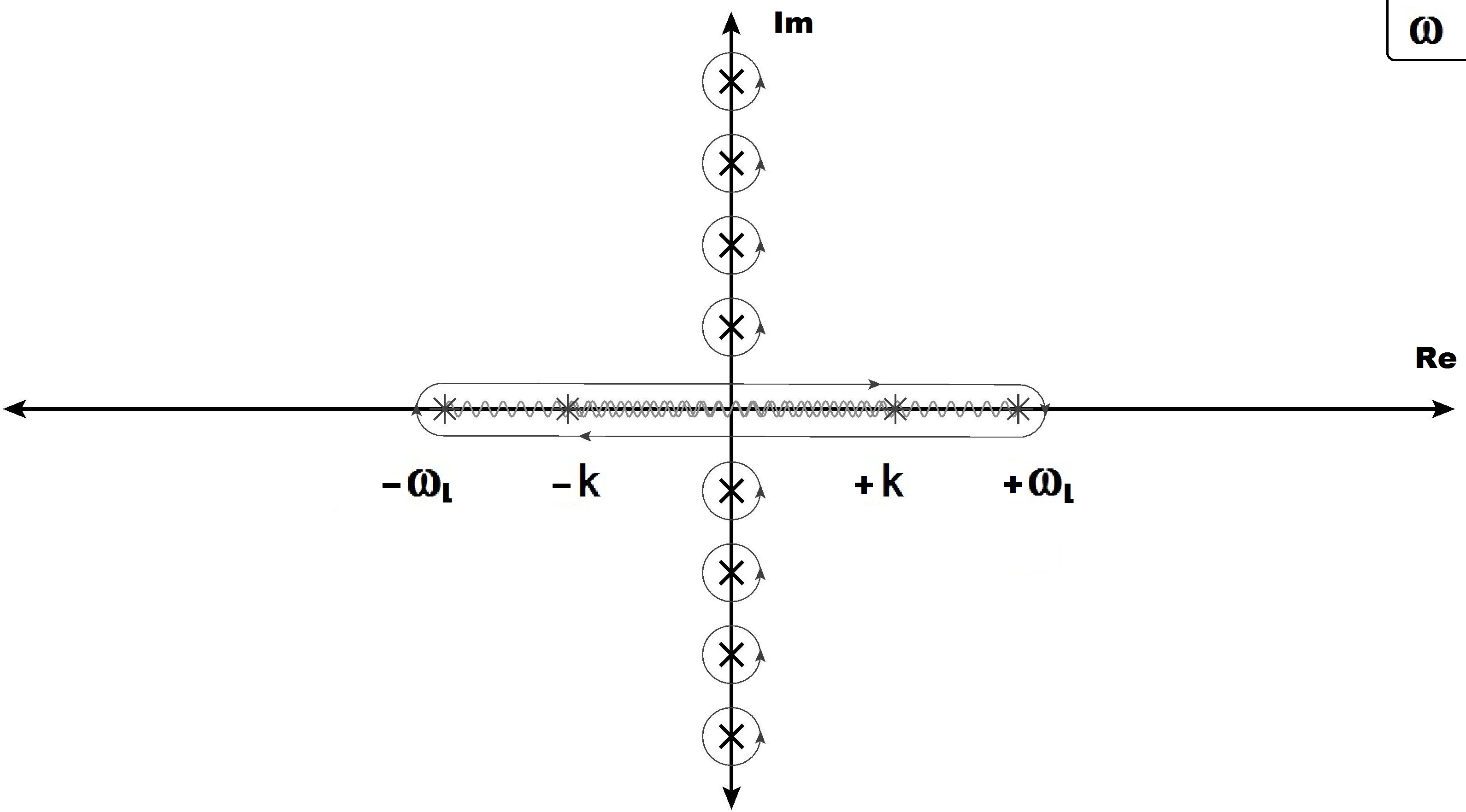
Refer to caption
Figure 9: Contours C,CL𝐶subscript𝐶LC,\,C_{\mbox{\scriptsize L}} and branch cuts of the longitudinal gluon contribution. See main text for details.

The contributions from the cuts are identified with the Landau damping part and the quasiparticle part, respectively. In analogy with the transverse gluon contribution, one finds

pLpLqp+pLLd,subscript𝑝Lsubscript𝑝subscriptLqpsubscript𝑝subscriptLLdp_{\mbox{\scriptsize L}}\equiv p_{{\mbox{\scriptsize L}}_{\mbox{\scriptsize qp}}}+p_{{\mbox{\scriptsize L}}_{\mbox{\scriptsize Ld}}}\,, (66)

with

pLqpsubscript𝑝subscriptLqp\displaystyle p_{{\mbox{\scriptsize L}}_{\mbox{\scriptsize qp}}} =\displaystyle= 𝐤{12(ωL(k)k)+Tlog(1eβωL1eβk)},subscript𝐤12subscript𝜔L𝑘𝑘𝑇1superscript𝑒𝛽subscript𝜔L1superscript𝑒𝛽𝑘\displaystyle-\int_{\bf k}\,\,\bigg{\{}\frac{1}{2}\left(\omega_{\mbox{\scriptsize L}}(k)-k\right)+T\,\log\left(\frac{1-e^{-\beta\omega_{\mbox{\scriptsize L}}}}{1-e^{-\beta k}}\right)\bigg{\}}\,, (67)

and

pLLdsubscript𝑝subscriptLLd\displaystyle p_{{\mbox{\scriptsize L}}_{\mbox{\scriptsize Ld}}} =\displaystyle= 𝐤0kdω{Discarctan[mD2Im{F12(12,1;32ϵ;k2ω2)}k2+mD2mD2Re{F12(12,1;32ϵ;k2ω2)}]\displaystyle\int_{\bf k}\,\int_{\kern-1.75pt\lower 3.5pt\hbox{\mbox{\scriptsize$0$}}}^{\kern-1.75pt\lower-3.5pt\hbox{\mbox{\scriptsize$k$}}}\kern-5.0pt\mbox{\normalsize$\mathop{{\rm d}\omega}$}\ \left\{{\rm Disc}\ \arctan\left[\frac{m_{\mbox{\scriptsize D}}^{2}\ \rm{Im}\ {\left\{{}_{2}F_{1}\left(\mbox{$\frac{1}{2},1;\frac{3}{2}-\epsilon;\frac{k^{2}}{\omega^{2}}$}\right)\right\}}}{k^{2}+m_{\mbox{\scriptsize D}}^{2}-m_{\mbox{\scriptsize D}}^{2}\ \rm{Re}\ {\left\{{}_{2}F_{1}\left(\mbox{$\frac{1}{2},1;\frac{3}{2}-\epsilon;\frac{k^{2}}{\omega^{2}}$}\right)\right\}}}\right]\right. (68)
×12π[1eβω1+12]..},\displaystyle\hskip 227.62204pt\,\times\left.\frac{1}{2\,\pi}\bigg{[}\frac{1}{e^{\beta\omega}-1}+\frac{1}{2}\bigg{]}\Bigg{.}\Bigg{.}\right\}\,,\ \ \ \ \ \ \ \ \ \

where both discontinuities are actually of the same type as for pTLdsubscript𝑝subscriptTLdp_{{\mbox{\scriptsize T}}_{\mbox{\scriptsize Ld}}}, and are therefore handled in a similar manner. Considering the Landau damping discontinuity, we also give details in appendix D. The dispersion relation is again considered in d=32ϵ𝑑32italic-ϵd=3-2\epsilon dimensions.

C.3 Quark contribution

Finally, let us consider the quark contribution which is given by eq. (11). As usual, by means of the contour trick, adding and subtracting the contribution to the pressure from an ideal gas of massless quarks leads to

pqfsubscript𝑝qf\displaystyle p_{\mbox{\scriptsize q${}_{f}$}} =\displaystyle= 2{K}log[k2+(ω~niμf)2]2subscript𝐾superscript𝑘2superscriptsubscript~𝜔𝑛𝑖subscript𝜇𝑓2\displaystyle 2\,\hbox{$\sum$}\!\!\!\!\!\!\!\int_{\{K\}}\log\Big{[}k^{2}+(\widetilde{\omega}_{n}-i\mu_{f})^{2}\Big{]} (69)
+2𝐤Tnlog[AS2(iω~n+μf,k)A02(iω~n+μf,k)k2(iω~n+μf)2]2subscript𝐤𝑇subscript𝑛superscriptsubscript𝐴S2𝑖subscript~𝜔𝑛subscript𝜇𝑓𝑘superscriptsubscript𝐴02𝑖subscript~𝜔𝑛subscript𝜇𝑓𝑘superscript𝑘2superscript𝑖subscript~𝜔𝑛subscript𝜇𝑓2\displaystyle\ \ \ \ \ +2\int_{\bf k}\,T\,\sum_{n}\log\left[\frac{A_{\mbox{\scriptsize S}}^{2}(i\widetilde{\omega}_{n}+\mu_{f},k)-A_{\mbox{\scriptsize 0}}^{2}(i\widetilde{\omega}_{n}+\mu_{f},k)}{k^{2}-(i\widetilde{\omega}_{n}+\mu_{f})^{2}}\right]\;
=\displaystyle= π2T445(74+30μ^f2+60μ^f4)superscript𝜋2superscript𝑇4457430superscriptsubscript^𝜇𝑓260superscriptsubscript^𝜇𝑓4\displaystyle\frac{\pi^{2}T^{4}}{45}\left(\frac{7}{4}+30\hat{\mu}_{f}^{2}+60\hat{\mu}_{f}^{4}\right)
+𝐤Cdω2πilog[AS2(ω,k)A02(ω,k)k2ω2]tanh(β(ωμf)2),subscript𝐤subscriptcontour-integral𝐶dω2πisuperscriptsubscript𝐴S2𝜔𝑘superscriptsubscript𝐴02𝜔𝑘superscript𝑘2superscript𝜔2𝛽𝜔subscript𝜇𝑓2\displaystyle\ \ \ \ \ +\int_{\bf k}\,\oint_{\lower 1.75pt\hbox{$\mbox{\tiny$C$}$}}\kern-2.5pt\mbox{\Large$\frac{\mathop{{\rm d}\omega}}{2\pi i}$}\kern 0.0pt\mbox{}\log\left[\frac{A_{\mbox{\scriptsize S}}^{2}(\omega,k)-A_{\mbox{\scriptsize 0}}^{2}(\omega,k)}{k^{2}-\omega^{2}}\right]\,\tanh\left(\frac{\beta\,(\omega-\mu_{f})}{2}\right)\,,

where the contour C𝐶C is shown in figure 10, and the flavor index f runs from 1 to Nfsubscript𝑁fN_{\mbox{\scriptsize f}}. The integrand has cuts starting at ±ωf±(k)plus-or-minussubscript𝜔subscript𝑓plus-or-minus𝑘\pm\omega_{\mbox{\scriptsize\tiny$f_{\pm}$}}(k), where ωf±(k)subscript𝜔subscript𝑓plus-or-minus𝑘\omega_{\mbox{\scriptsize\tiny$f_{\pm}$}}(k) are the quasiparticle dispersion relations for quarks and plasminos, satisfying

0A0(ωf±,k)AS(ωf±,k).0minus-or-plussubscript𝐴0subscript𝜔subscript𝑓plus-or-minus𝑘subscript𝐴Ssubscript𝜔subscript𝑓plus-or-minus𝑘0\equiv A_{\mbox{\scriptsize 0}}(\omega_{\mbox{\scriptsize\tiny$f_{\pm}$}},k)\mp A_{\mbox{\scriptsize S}}(\omega_{\mbox{\scriptsize\tiny$f_{\pm}$}},k)\;. (70)

The integrand has another set of cuts starting at ±kplus-or-minus𝑘\pm k. We choose the cuts to run from the branch points as shown in figure 10.
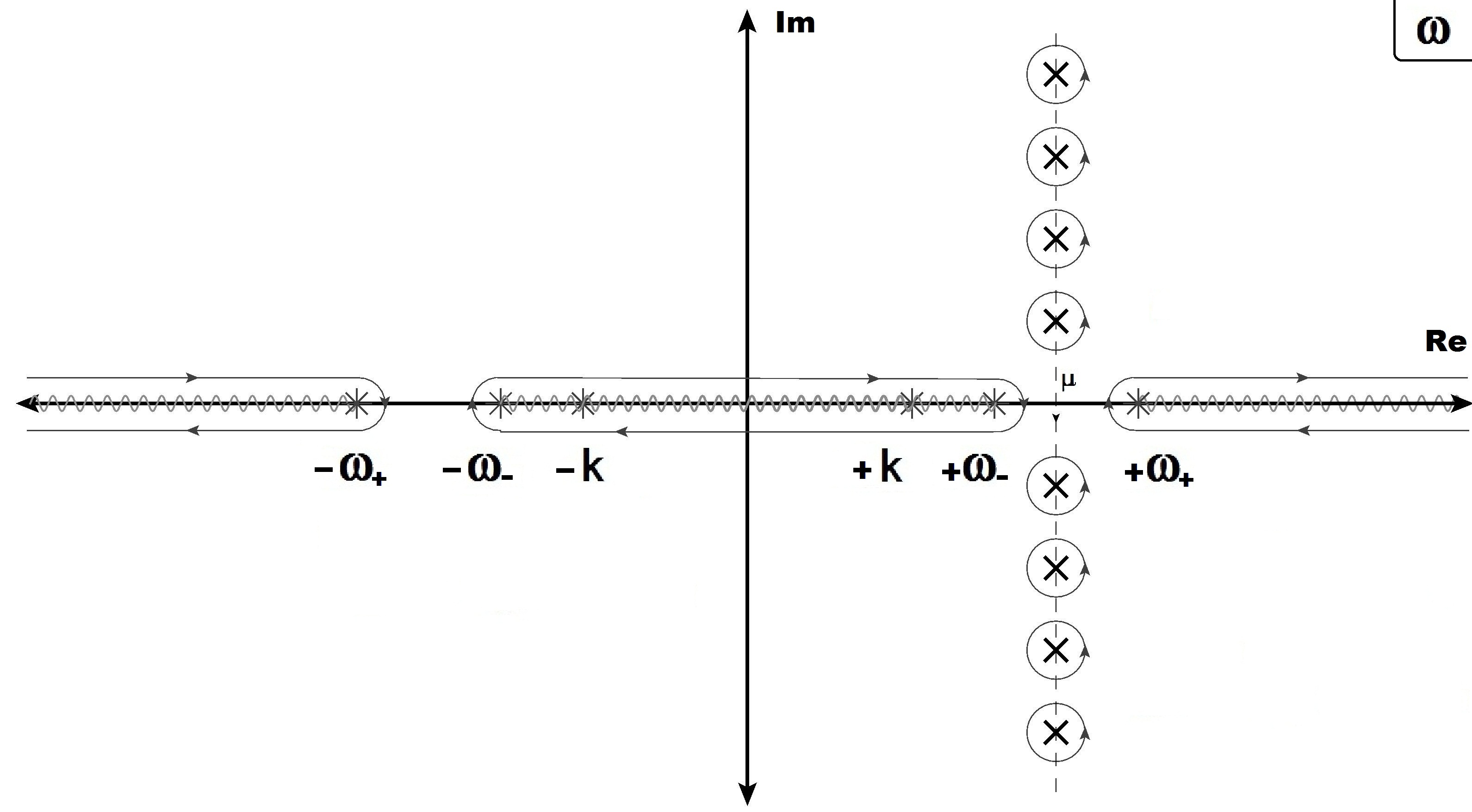
Refer to caption
Figure 10: Contours C,Cq𝐶subscript𝐶qC,\,C_{\mbox{\scriptsize q}} and branch cuts of the quark contribution. See main text for details.

The contour is finally deformed to wrap around the cuts and gives Cqsubscript𝐶qC_{\mbox{\scriptsize q}}. After collapsing it onto the branch cuts, the quark contribution to the pressure can be written as

pqfpqqpf+pqLdf,subscript𝑝qfsubscript𝑝subscriptqsubscriptqp𝑓subscript𝑝subscriptqsubscriptLd𝑓p_{\mbox{\scriptsize q${}_{f}$}}\equiv p_{{\mbox{\scriptsize q}}_{{\mbox{\scriptsize qp}}_{f}}}+p_{{\mbox{\scriptsize q}}_{{\mbox{\scriptsize Ld}}_{f}}}\,, (71)

with

pqqpfsubscript𝑝subscriptqsubscriptqp𝑓\displaystyle p_{{\mbox{\scriptsize q}}_{{\mbox{\scriptsize qp}}_{f}}} =\displaystyle= 2𝐤{Tlog(1+eβ(ωf++μf))+Tlog(1+eβ(ωf+μf))\displaystyle 2\int_{\bf k}\,\,\bigg{\{}T\,\log\left(1+e^{-\beta\left(\omega_{f_{+}}+\mu_{f}\right)}\right)+T\,\log\left(1+e^{-\beta\left(\omega_{f_{+}}-\mu_{f}\right)}\right) (72)
+Tlog(1+eβ(ωf+μf)1+eβ(k+μf))+Tlog(1+eβ(ωfμf)1+eβ(kμf))}\displaystyle\ \ \ \ \ \ \ \ \ +T\,\log\left(\frac{1+e^{-\beta\left(\omega_{f_{-}}+\mu_{f}\right)}}{1+e^{-\beta(k+\mu_{f})}}\right)+T\,\log\left(\frac{1+e^{-\beta\left(\omega_{f_{-}}-\mu_{f}\right)}}{1+e^{-\beta(k-\mu_{f})}}\right)\bigg{\}}
+\displaystyle+ 2𝐤{ωf+(k)+(ωf(k)k)},2subscript𝐤subscript𝜔subscript𝑓𝑘subscript𝜔subscript𝑓𝑘𝑘\displaystyle 2\int_{\bf k}\,\,\bigg{\{}\omega_{f_{+}}(k)+\left(\omega_{f_{-}}(k)-k\right)\bigg{\}}\,,

and

pqLdfsubscript𝑝subscriptqsubscriptLd𝑓\displaystyle p_{{\mbox{\scriptsize q}}_{{\mbox{\scriptsize Ld}}_{f}}} =\displaystyle= 1π𝐤0kdω{Discθqf,ϵ[1eβ(ω+μf)+1+1eβ(ωμf)+11]},1𝜋subscript𝐤superscriptsubscript0𝑘d𝜔Discsubscript𝜃qf,ϵdelimited-[]1superscript𝑒𝛽𝜔subscript𝜇𝑓11superscript𝑒𝛽𝜔subscript𝜇𝑓11\displaystyle\frac{1}{\pi}\int_{\bf k}\,\int_{\kern-1.75pt\lower 3.5pt\hbox{\mbox{\scriptsize$0$}}}^{\kern-1.75pt\lower-3.5pt\hbox{\mbox{\scriptsize$k$}}}\kern-5.0pt\mbox{\normalsize$\mathop{{\rm d}\omega}$}\ \left\{{\rm Disc}\ \theta_{\mbox{\scriptsize q${}_{f}$,$\epsilon$}}\,\bigg{[}\frac{1}{e^{\beta(\omega+\mu_{f})}+1}+\frac{1}{e^{\beta(\omega-\mu_{f})}+1}-1\bigg{]}\right\}\;, (73)

where θqf,ϵarctan[Ξf,ϵ]subscript𝜃qf,ϵsubscriptΞf,ϵ\theta_{\mbox{\scriptsize q${}_{f}$,$\epsilon$}}\equiv\arctan\left[\Xi_{\mbox{\scriptsize$f$,$\epsilon$}}\right], with its argument defined as

Ξf,ϵsubscriptΞf,ϵabsent\displaystyle\Xi_{\mbox{\scriptsize$f$,$\epsilon$}}\equiv (74)
mqf4k2[2Im{F12(12,1;32ϵ;k2ω2)}+k2ω2ω2Im{F12(12,1;32ϵ;k2ω2)2}]k2ω2+2mqf2+mqf4k2[12Re{F12(12,1;32ϵ;k2ω2)}k2ω2ω2Re{F12(12,1;32ϵ;k2ω2)2}].superscriptsubscript𝑚subscript𝑞𝑓4superscript𝑘2delimited-[]2ImsubscriptsubscriptF1212132italic-ϵsuperscript𝑘2superscript𝜔2superscriptk2superscript𝜔2superscript𝜔2ImsubscriptsubscriptF12superscript12132italic-ϵsuperscript𝑘2superscript𝜔22superscript𝑘2superscript𝜔22superscriptsubscript𝑚subscript𝑞𝑓2superscriptsubscript𝑚subscript𝑞𝑓4superscript𝑘2delimited-[]12ResubscriptsubscriptF1212132italic-ϵsuperscript𝑘2superscript𝜔2superscriptk2superscript𝜔2superscript𝜔2ResubscriptsubscriptF12superscript12132italic-ϵsuperscript𝑘2superscript𝜔22\displaystyle\frac{\frac{m_{q_{\mbox{\tiny$f$}}}^{4}}{k^{2}}\left[2\ \rm{Im}\ {\left\{{}_{2}F_{1}\left(\mbox{$\frac{1}{2},1;\frac{3}{2}-\epsilon;\frac{k^{2}}{\omega^{2}}$}\right)\right\}}+\frac{k^{2}-\omega^{2}}{\omega^{2}}\ \rm{Im}\ {\left\{{}_{2}F_{1}\left(\mbox{$\frac{1}{2},1;\frac{3}{2}-\epsilon;\frac{k^{2}}{\omega^{2}}$}\right)^{2}\right\}}\right]}{k^{2}-\omega^{2}+2m_{q_{\mbox{\tiny$f$}}}^{2}+\frac{m_{q_{\mbox{\tiny$f$}}}^{4}}{k^{2}}\,\left[1-2\,\rm{Re}\ {\left\{{}_{2}F_{1}\left(\mbox{$\frac{1}{2},1;\frac{3}{2}-\epsilon;\frac{k^{2}}{\omega^{2}}$}\right)\right\}}-\frac{k^{2}-\omega^{2}}{\omega^{2}}\,\rm{Re}\ {\left\{{}_{2}F_{1}\left(\mbox{$\frac{1}{2},1;\frac{3}{2}-\epsilon;\frac{k^{2}}{\omega^{2}}$}\right)^{2}\right\}}\right]}\;.\ \ \ \ \

The subscript ϵitalic-ϵ\epsilon stands to remind that these quantities are considered in d=32ϵ𝑑32italic-ϵd=3-2\epsilon dimensions, as for the dispersion relations. Again, both discontinuities are of the same type as for pTLdsubscript𝑝subscriptTLdp_{{\mbox{\scriptsize T}}_{\mbox{\scriptsize Ld}}} and pLLdsubscript𝑝subscriptLLdp_{{\mbox{\scriptsize L}}_{\mbox{\scriptsize Ld}}}, and have to be handled in a similar manner. We refer to appendix D for more details about the Landau damping discontinuity.

C.4 Renormalization

The expressions for pTsubscript𝑝Tp_{\mbox{\scriptsize T}}, pLsubscript𝑝Lp_{\mbox{\scriptsize L}}, and pqfsubscript𝑝qfp_{\mbox{\scriptsize q${}_{f}$}} given by eqs. (59), (61), (67), (68), (72), and (73) are UV divergent and are regulated by using dimensional regularization in d=32ϵ𝑑32italic-ϵd=3-2\epsilon dimensions. Some of the divergences are explicitly independent of temperature and chemical potentials, while others depend on the temperature and the chemical potentials via the Bose-Einstein and Fermi-Dirac distribution functions. The strategy will be to first calculate the divergences of the temperature and chemical potential dependent terms, and then calculate the terms that are explicitly independent of (T,𝝁)𝑇𝝁(T,\,{\bm{\mu}}), by taking the limits T0𝑇0T\rightarrow 0 and 𝝁0𝝁0{\bm{\mu}}\rightarrow 0.

We first consider the second term in eqs. (67). This term is finite and we therefore just keep it as it stands. The next term is the temperature dependent piece of the Landau damping contribution in eq. (68), and reads

12π𝐤0kdω{Discarctan[mD2Im{F12(12,1;32ϵ;k2ω2)}k2+mD2mD2Re{F12(12,1;32ϵ;k2ω2)}]1eβω1..}.\displaystyle\frac{1}{2\,\pi}\int_{\bf k}\,\int_{\kern-1.75pt\lower 3.5pt\hbox{\mbox{\scriptsize$0$}}}^{\kern-1.75pt\lower-3.5pt\hbox{\mbox{\scriptsize$k$}}}\kern-5.0pt\mbox{\normalsize$\mathop{{\rm d}\omega}$}\ \left\{{\rm Disc}\ \arctan\left[\frac{m_{\mbox{\scriptsize D}}^{2}\ \rm{Im}\ {\left\{{}_{2}F_{1}\left(\mbox{$\frac{1}{2},1;\frac{3}{2}-\epsilon;\frac{k^{2}}{\omega^{2}}$}\right)\right\}}}{k^{2}+m_{\mbox{\scriptsize D}}^{2}-m_{\mbox{\scriptsize D}}^{2}\ \rm{Re}\ {\left\{{}_{2}F_{1}\left(\mbox{$\frac{1}{2},1;\frac{3}{2}-\epsilon;\frac{k^{2}}{\omega^{2}}$}\right)\right\}}}\right]\,\,\frac{1}{e^{\beta\omega}-1}\Bigg{.}\Bigg{.}\right\}\;.\ \ \ \ \ \ \ \ \ \ (75)

In ref. Jens2 , this term was analyzed with the integrand directly in d=3𝑑3d=3 dimensions, and it was shown that UV divergences appear for k𝑘k\rightarrow\infty with ω𝜔\omega fixed. A similar analysis can be carried out here (i.e. in d=32ϵ𝑑32italic-ϵd=3-2\epsilon dimensions), by noticing that

DiscIm{F12(12,1;32ϵ;k2ω2)}DiscImsubscriptsubscriptF1212132italic-ϵsuperscript𝑘2superscript𝜔2\displaystyle{\rm Disc}\ \rm{Im}\ {\left\{{}_{2}F_{1}\left(\mbox{$\frac{1}{2},1;\frac{3}{2}-\epsilon;\frac{k^{2}}{\omega^{2}}$}\right)\right\}} =kω fixedω fixed𝑘\displaystyle\underset{\underset{\mbox{\tiny$\omega$ fixed}}{k\longrightarrow\infty}}{=}  4Γ(32ϵ)Γ(32)Γ(1ϵ)ωk+𝒪(ω2k2).4Γ32italic-ϵΓ32Γ1italic-ϵ𝜔𝑘𝒪superscript𝜔2superscript𝑘2\displaystyle-\,4\,\,\frac{\Gamma\left(\frac{3}{2}-\epsilon\right)\,\Gamma\left(\frac{3}{2}\right)}{\Gamma\left(1-\epsilon\right)}\,\frac{\omega}{k}+{\cal O}\left(\frac{\omega^{2}}{k^{2}}\right)\;. (76)

We refer to appendix D for details on the computation of the branch cut discontinuity of the imaginary part of this hypergeometric function, in its assymptotic expansion.

By Taylor expanding the integrand in eq. (75) around k=+𝑘k=+\infty, using eq. (76), we obtain an integral which contains the relevant UV divergences in three dimensions, and reads

𝒟LLdsubscript𝒟subscriptLLd\displaystyle\mathcal{D}_{{\mbox{\scriptsize L}}_{\mbox{\scriptsize Ld}}} \displaystyle\equiv 2mD2πΓ(32ϵ)Γ(32)Γ(1ϵ)𝐤0kdω{ωk31eβω1..}.\displaystyle-\frac{2\,m_{\mbox{\scriptsize D}}^{2}}{\pi}\,\,\frac{\Gamma\left(\frac{3}{2}-\epsilon\right)\Gamma\left(\frac{3}{2}\right)}{\Gamma\left(1-\epsilon\right)}\int_{\bf k}\,\int_{\kern-1.75pt\lower 3.5pt\hbox{\mbox{\scriptsize$0$}}}^{\kern-1.75pt\lower-3.5pt\hbox{\mbox{\scriptsize$k$}}}\kern-5.0pt\mbox{\normalsize$\mathop{{\rm d}\omega}$}\ \left\{\frac{\omega}{k^{3}}\,\,\frac{1}{e^{\beta\omega}-1}\Bigg{.}\Bigg{.}\right\}\;. (77)

This integral can be easily evaluated, and the result through 𝒪(ϵ0)𝒪superscriptitalic-ϵ0{\cal O}\left(\epsilon^{0}\right) is

𝒟LLdsubscript𝒟subscriptLLd\displaystyle\mathcal{D}_{{\mbox{\scriptsize L}}_{\mbox{\scriptsize Ld}}} =\displaystyle= mD2T248[1ϵ+2log(Λ2πT)+2ζ(1)ζ(1)+𝒪(ϵ)].superscriptsubscript𝑚D2superscript𝑇248delimited-[]1italic-ϵ2Λ2𝜋𝑇2superscript𝜁1𝜁1𝒪italic-ϵ\displaystyle\frac{m_{\mbox{\scriptsize D}}^{2}\,T^{2}}{48}\,\left[\frac{1}{\epsilon}+2\log\left(\frac{\Lambda}{2\pi T}\right)+2\,\,\frac{\zeta^{\prime}\left(-1\right)}{\zeta\left(-1\right)}+{\cal O}\left(\epsilon\right)\right]\;. (78)

Similarly, the temperature dependent term from the transverse gluon contribution (59) is

12π𝐤0kdω{Discarctan[mD222ϵk2ω2k2Im{F12(12,1;32ϵ;k2ω2)}k2ω2+mD222ϵω2k2[1+k2ω2ω2Re{F12(12,1;32ϵ;k2ω2)}]]\displaystyle-\frac{1}{2\,\pi}\int_{\bf k}\,\int_{\kern-1.75pt\lower 3.5pt\hbox{\mbox{\scriptsize$0$}}}^{\kern-1.75pt\lower-3.5pt\hbox{\mbox{\scriptsize$k$}}}\kern-5.0pt\mbox{\normalsize$\mathop{{\rm d}\omega}$}\ \left\{{\rm Disc}\ \arctan\left[\frac{\frac{m_{\mbox{\scriptsize D}}^{2}}{2-2\epsilon}\frac{k^{2}-\omega^{2}}{k^{2}}\ \rm{Im}\ {\left\{{}_{2}F_{1}\left(\mbox{$\frac{1}{2},1;\frac{3}{2}-\epsilon;\frac{k^{2}}{\omega^{2}}$}\right)\right\}}}{k^{2}-\omega^{2}+\frac{m_{\mbox{\scriptsize D}}^{2}}{2-2\epsilon}\frac{\omega^{2}}{k^{2}}\left[1+\frac{k^{2}-\omega^{2}}{\omega^{2}}\ \rm{Re}\ {\left\{{}_{2}F_{1}\left(\mbox{$\frac{1}{2},1;\frac{3}{2}-\epsilon;\frac{k^{2}}{\omega^{2}}$}\right)\right\}}\right]}\right]\right.
×[1eβω1]..}.\displaystyle\hskip 227.62204pt\,\left.\times\bigg{[}\frac{1}{e^{\beta\omega}-1}\bigg{]}\Bigg{.}\Bigg{.}\right\}\;. (79)

This leads to the integral

𝒟TLdsubscript𝒟subscriptTLd\displaystyle\mathcal{D}_{{\mbox{\scriptsize T}}_{\mbox{\scriptsize Ld}}} \displaystyle\equiv mD2πΓ(32ϵ)Γ(32)(1ϵ)Γ(1ϵ)𝐤0kdω{ωk31eβω1..},\displaystyle\frac{m_{\mbox{\scriptsize D}}^{2}}{\pi}\,\,\frac{\Gamma\left(\frac{3}{2}-\epsilon\right)\Gamma\left(\frac{3}{2}\right)}{(1-\epsilon)\,\Gamma\left(1-\epsilon\right)}\int_{\bf k}\,\int_{\kern-1.75pt\lower 3.5pt\hbox{\mbox{\scriptsize$0$}}}^{\kern-1.75pt\lower-3.5pt\hbox{\mbox{\scriptsize$k$}}}\kern-5.0pt\mbox{\normalsize$\mathop{{\rm d}\omega}$}\ \left\{\frac{\omega}{k^{3}}\,\,\frac{1}{e^{\beta\omega}-1}\Bigg{.}\Bigg{.}\right\}\,, (80)

which through 𝒪(ϵ0)𝒪superscriptitalic-ϵ0{\cal O}\left(\epsilon^{0}\right) reads

𝒟TLdsubscript𝒟subscriptTLd\displaystyle\mathcal{D}_{{\mbox{\scriptsize T}}_{\mbox{\scriptsize Ld}}} =\displaystyle= mD2T296[1ϵ+1+2log(Λ2πT)+2ζ(1)ζ(1)+𝒪(ϵ)].superscriptsubscript𝑚D2superscript𝑇296delimited-[]1italic-ϵ12Λ2𝜋𝑇2superscript𝜁1𝜁1𝒪italic-ϵ\displaystyle-\frac{m_{\mbox{\scriptsize D}}^{2}\,T^{2}}{96}\,\left[\frac{1}{\epsilon}+1+2\log\left(\frac{\Lambda}{2\pi\,T}\right)+2\,\,\frac{\zeta^{\prime}\left(-1\right)}{\zeta\left(-1\right)}+{\cal O}\left(\epsilon\right)\right]\;. (81)

We notice that the divergences in eqs. (78) and (81) cancel in the combination

dA[(22ϵ)𝒟TLd+𝒟LLd]=𝒪(ϵ),subscript𝑑Adelimited-[]22italic-ϵsubscript𝒟subscriptTLdsubscript𝒟subscriptLLd𝒪italic-ϵd_{\mbox{\scriptsize A}}\Big{[}(2-2\epsilon)\ \mathcal{D}_{{\mbox{\scriptsize T}}_{\mbox{\scriptsize Ld}}}+\mathcal{D}_{{\mbox{\scriptsize L}}_{\mbox{\scriptsize Ld}}}\Big{]}={\cal O}\left(\epsilon\right)\;, (82)

which is actually the one given by eq. (8). Hence, there is no need for adding and subtracting an integral for the Landau damping divergent pieces in pTsubscript𝑝Tp_{\mbox{\scriptsize T}} and pLsubscript𝑝Lp_{\mbox{\scriptsize L}}, in order to renormalize the result for the gluon Landau damping contribution.

Let us finally discuss the quark terms given by eqs. (72) and (73). In eq. (72), the only divergent term involves the dispersion relation ωf+(k)subscript𝜔subscript𝑓𝑘\omega_{f_{+}}(k) and is independent of T𝑇T and 𝝁𝝁\bm{\mu}. Thus, we will deal with it later. In eq. (73), there are no divergent terms, even when k𝑘k\rightarrow\infty with fixed ω𝜔\omega, since the expansion of eq. (C.3) starts to contribute at 𝒪(mqf2ω/k3)𝒪superscriptsubscript𝑚subscript𝑞𝑓2𝜔superscript𝑘3{\cal O}({m_{q_{f}}^{2}{\omega}/k^{3}}) instead of 𝒪(ω/k)𝒪𝜔𝑘{\cal O}({\omega/k}).

The fact that all the temperature dependent divergences cancel, and that there is no divergence dependent on the quark chemical potentials, allows us to write the one-loop pressure as follows

pHTLpt(T,𝝁)subscript𝑝HTLpt𝑇𝝁\displaystyle p_{\mbox{\scriptsize HTLpt}}\left(T,\bm{\mu}\right) =\displaystyle= dA{(22ϵ)T𝐤log(1eβωT)T𝐤log(1eβωL1eβk)+pL\displaystyle d_{\mbox{\scriptsize A}}\Bigg{\{}-(2-2\epsilon)\,T\int_{\bf k}\log\bigg{(}1-e^{-\beta\omega_{\mbox{\scriptsize T}}}\bigg{)}-\,T\int_{\bf k}\log\bigg{(}\frac{1-e^{-\beta\omega_{\mbox{\scriptsize L}}}}{1-e^{-\beta\,k}}\bigg{)}+\ p^{\star}_{\mbox{\scriptsize L}} (83)
+(22ϵ)pT12π𝐤0kdω[(22ϵ)DiscϕT,ϵDiscϕL,ϵ]1eβω1}\displaystyle\ \ \ \ +\ (2-2\epsilon)\,p^{\star}_{\mbox{\scriptsize T}}-\frac{1}{2\,\pi}\int_{\bf k}\,\int_{\kern-1.75pt\lower 3.5pt\hbox{\mbox{\scriptsize$0$}}}^{\kern-1.75pt\lower-3.5pt\hbox{\mbox{\scriptsize$k$}}}\kern-5.0pt\mbox{\normalsize$\mathop{{\rm d}\omega}$}\ \bigg{[}(2-2\epsilon)\,{\rm Disc}\ \phi_{{\mbox{\scriptsize T}},\epsilon}-{\rm Disc}\ \phi_{{\mbox{\scriptsize L}},\epsilon}\bigg{]}\,\,\frac{1}{e^{\beta\omega}-1}\Bigg{\}}
+\displaystyle+ Ncf,s=±1{2T𝐤log[1+eβ(ωf++sμf)]+2T𝐤log[1+eβ(ωf+sμf)1eβ(k+sμf)]\displaystyle N_{\mbox{\scriptsize c}}\sum_{f,\,s=\pm 1}\Bigg{\{}2\,T\int_{\bf k}\log\bigg{[}1+e^{-\beta\left(\omega_{f_{+}}+s\,\mu_{f}\right)}\bigg{]}+2\,T\int_{\bf k}\log\left[\frac{1+e^{-\beta\left(\omega_{f_{-}}+s\,\mu_{f}\right)}}{1-e^{-\beta\left(k+s\,\mu_{f}\right)}}\right]
+pqf2+1π𝐤0kdωDiscθqf,ϵ[1eβ(ω+sμf)+1]}+Δp,\displaystyle\ \ \ \ \ \ \ \ \ +\ \frac{p^{\star}_{\mbox{\scriptsize q${}_{f}$}}}{2}+\frac{1}{\pi}\,\int_{\bf k}\,\int_{\kern-1.75pt\lower 3.5pt\hbox{\mbox{\scriptsize$0$}}}^{\kern-1.75pt\lower-3.5pt\hbox{\mbox{\scriptsize$k$}}}\kern-5.0pt\mbox{\normalsize$\mathop{{\rm d}\omega}$}\ \,\,{\rm Disc}\ \theta_{\mbox{\scriptsize q${}_{f}$,$\epsilon$}}\left[\frac{1}{{e^{\beta\left(\omega+s\,\mu_{f}\right)}+1}}\right]\Bigg{\}}+\Delta p\;,

where the subscript ϵitalic-ϵ\epsilon in ϕT,ϵsubscriptitalic-ϕTitalic-ϵ\phi_{{\mbox{\scriptsize T}},\epsilon} and ϕL,ϵsubscriptitalic-ϕLitalic-ϵ\phi_{{\mbox{\scriptsize L}},\epsilon} serves to remind us that these angles, respectively corresponding to the arctan\arctan functions in eqs. (59) and (68), are considered in d=32ϵ𝑑32italic-ϵd=3-2\epsilon dimensions. Note also that the dispersion relations are still in d=32ϵ𝑑32italic-ϵd=3-2\epsilon dimensions.

The terms pTsubscriptsuperscript𝑝Tp^{\star}_{\mbox{\scriptsize T}}, pLsubscriptsuperscript𝑝Lp^{\star}_{\mbox{\scriptsize L}}, and pqfsubscriptsuperscript𝑝qfp^{\star}_{\mbox{\scriptsize q${}_{f}$}} are the terms from pTsubscript𝑝Tp_{\mbox{\scriptsize T}}, pLsubscript𝑝Lp_{\mbox{\scriptsize L}}, and pqfsubscript𝑝qfp_{\mbox{\scriptsize q${}_{f}$}} that are explicitly independent of T𝑇T and 𝝁𝝁{\bm{\mu}}. They contain all the UV divergences. Moreover, pLsubscriptsuperscript𝑝Lp^{\star}_{\mbox{\scriptsize L}} also contains the finite contribution coming from the integral over (ωL(k)k)/2subscript𝜔L𝑘𝑘2(\omega_{\mbox{\scriptsize L}}(k)-k)/2, and pqfsubscriptsuperscript𝑝qfp^{\star}_{\mbox{\scriptsize q${}_{f}$}} contains the finite contribution coming from the integral over (ωf(k)k)subscript𝜔subscript𝑓𝑘𝑘(\omega_{f_{-}}(k)-k), since both are explicitly temperature and chemical potential independent. We need therefore to compute them.

In the limit T0𝑇0T\rightarrow 0, the transverse gluon term pTsubscript𝑝Tp_{\mbox{\scriptsize T}} approaches pTsubscriptsuperscript𝑝Tp^{\star}_{\mbox{\scriptsize T}} and can be expressed as an integral over continuous Euclidean energy, which we denote ωEsubscript𝜔E\omega_{\mbox{\scriptsize E}}. We find

pT=14π+dωE𝐤log[k2+ωE2+ΠT(iωE,k)].subscriptsuperscript𝑝T14𝜋superscriptsubscriptdsubscript𝜔Esubscript𝐤superscript𝑘2superscriptsubscript𝜔E2subscriptΠT𝑖subscript𝜔E𝑘p^{\star}_{\mbox{\scriptsize T}}=-\frac{1}{4\,\pi}\int_{\kern-1.75pt\lower 3.5pt\hbox{\mbox{\scriptsize$-\infty$}}}^{\kern-1.75pt\lower-3.5pt\hbox{\mbox{\scriptsize$+\infty$}}}\kern-7.5pt\mbox{\normalsize$\mathop{{\rm d}\omega_{\mbox{\scriptsize E}}}$}\int_{\bf k}\,\log\Big{[}k^{2}+\omega_{\mbox{\scriptsize E}}^{2}+\Pi_{\mbox{\scriptsize T}}(i\omega_{\mbox{\scriptsize E}},k)\Big{]}\,. (84)

It is then convenient to rescale the Euclidean energy as ωEkωEsubscript𝜔E𝑘subscript𝜔E\omega_{\mbox{\scriptsize E}}\rightarrow k\,\omega_{\mbox{\scriptsize E}}. This yields

pT=12π0dωE𝐤klog[(1+ωE2)k2+ΠT(iωE,1)].subscriptsuperscript𝑝T12𝜋superscriptsubscript0dsubscript𝜔Esubscript𝐤𝑘1superscriptsubscript𝜔E2superscript𝑘2subscriptΠT𝑖subscript𝜔E1p^{\star}_{\mbox{\scriptsize T}}=-\frac{1}{2\,\pi}\int_{\kern-1.75pt\lower 3.5pt\hbox{\mbox{\scriptsize$0$}}}^{\kern-1.75pt\lower-3.5pt\hbox{\mbox{\scriptsize$\infty$}}}\kern-7.5pt\mbox{\normalsize$\mathop{{\rm d}\omega_{\mbox{\scriptsize E}}}$}\int_{\bf k}\,k\log\Big{[}(1+\omega_{\mbox{\scriptsize E}}^{2})\,k^{2}+\Pi_{\mbox{\scriptsize T}}(i\omega_{\mbox{\scriptsize E}},1)\Big{]}\,. (85)

Similarly, the rescaled expressions for the longitudinal gluon contribution (10) and the quark contribution (11), taking the limit 𝝁0𝝁0{\bm{\mu}}\rightarrow 0, are

pLsubscriptsuperscript𝑝L\displaystyle p^{\star}_{\mbox{\scriptsize L}} =\displaystyle= 12π0dωE𝐤klog[k2+ΠL(iωE,1)],12𝜋superscriptsubscript0dsubscript𝜔Esubscript𝐤𝑘superscript𝑘2subscriptΠL𝑖subscript𝜔E1\displaystyle-\frac{1}{2\,\pi}\int_{\kern-1.75pt\lower 3.5pt\hbox{\mbox{\scriptsize$0$}}}^{\kern-1.75pt\lower-3.5pt\hbox{\mbox{\scriptsize$\infty$}}}\kern-7.5pt\mbox{\normalsize$\mathop{{\rm d}\omega_{\mbox{\scriptsize E}}}$}\int_{\bf k}\,k\,\log\Big{[}k^{2}+\Pi_{\mbox{\scriptsize L}}(i\omega_{\mbox{\scriptsize E}},1)\Big{]}\,, (86)
pqfsubscriptsuperscript𝑝qf\displaystyle p^{\star}_{\mbox{\scriptsize q${}_{f}$}} =\displaystyle= 2π0dωE𝐤klog[(1+mqf2k2{11+iωE𝒯~K(iωE,1)iωE})\displaystyle\frac{2}{\pi}\int_{\kern-1.75pt\lower 3.5pt\hbox{\mbox{\scriptsize$0$}}}^{\kern-1.75pt\lower-3.5pt\hbox{\mbox{\scriptsize$\infty$}}}\kern-7.5pt\mbox{\normalsize$\mathop{{\rm d}\omega_{\mbox{\scriptsize E}}}$}\int_{\bf k}\,k\,\log\left[\left(1+\frac{m_{\mbox{\scriptsize q${}_{f}$}}^{2}}{k^{2}}\,\left\{\frac{1}{1+i\,\omega_{\mbox{\scriptsize E}}}-\frac{\widetilde{{\cal T}}_{\mbox{\scriptsize K}}(i\omega_{\mbox{\scriptsize E}},1)}{i\,\omega_{\mbox{\scriptsize E}}}\right\}\right)\right. (87)
×(1+mqf2k2{11iωE+𝒯~K(iωE,1)iωE})].\displaystyle\ \ \ \ \ \ \ \ \ \ \ \ \ \ \ \ \ \ \ \ \ \ \ \ \ \ \ \times\left.\left(1+\frac{m_{\mbox{\scriptsize q${}_{f}$}}^{2}}{k^{2}}\,\left\{\frac{1}{1-i\,\omega_{\mbox{\scriptsize E}}}+\frac{\widetilde{{\cal T}}_{\mbox{\scriptsize K}}(i\omega_{\mbox{\scriptsize E}},1)}{i\,\omega_{\mbox{\scriptsize E}}}\right\}\right)\right]\,.

For the latter, notice that before rescaling, we added and subtracted a log(k2+ωE2)superscript𝑘2superscriptsubscript𝜔E2\log\left(k^{2}+\omega_{\mbox{\scriptsize E}}^{2}\right) term to the main logarithm in eq. (87). The added piece is computed directly and vanishes thanks to dimensional regularization. The subtracted one is combined with the main log\log for convenience during manipulations of its argument. Integrating over k𝑘k, we obtain

pTsubscriptsuperscript𝑝T\displaystyle p^{\star}_{\mbox{\scriptsize T}} =\displaystyle= eγEϵΛ¯2ϵ16π5/2Γ(2ϵ)Γ(ϵ2)Γ(32ϵ)0dωE(ΠT(iωE,1)1+ωE2)2ϵ,superscript𝑒subscript𝛾Eitalic-ϵsuperscript¯Λ2italic-ϵ16superscript𝜋52Γ2italic-ϵΓitalic-ϵ2Γ32italic-ϵsuperscriptsubscript0dsubscript𝜔EsuperscriptsubscriptΠT𝑖subscript𝜔E11superscriptsubscript𝜔E22italic-ϵ\displaystyle\frac{e^{\gamma_{\mbox{\scriptsize\tiny E}}\epsilon}\,\bar{\Lambda}^{2\epsilon}}{16\,\pi^{5/2}}\,\,\frac{\Gamma\left(2-\epsilon\right)\Gamma\left(\epsilon-2\right)}{\Gamma\left(\frac{3}{2}-\epsilon\right)}\int_{\kern-1.75pt\lower 3.5pt\hbox{\mbox{\scriptsize$0$}}}^{\kern-1.75pt\lower-3.5pt\hbox{\mbox{\scriptsize$\infty$}}}\kern-7.5pt\mbox{\normalsize$\mathop{{\rm d}\omega_{\mbox{\scriptsize E}}}$}\,\left(\frac{\Pi_{\mbox{\scriptsize T}}(i\omega_{\mbox{\scriptsize E}},1)}{1+\omega_{\mbox{\scriptsize E}}^{2}}\right)^{2-\epsilon}\,, (88)
pLsubscriptsuperscript𝑝L\displaystyle p^{\star}_{\mbox{\scriptsize L}} =\displaystyle= eγEϵΛ¯2ϵ16π5/2Γ(2ϵ)Γ(ϵ2)Γ(32ϵ)0dωE(ΠL(iωE,1))2ϵ,superscript𝑒subscript𝛾Eitalic-ϵsuperscript¯Λ2italic-ϵ16superscript𝜋52Γ2italic-ϵΓitalic-ϵ2Γ32italic-ϵsuperscriptsubscript0dsubscript𝜔EsuperscriptsubscriptΠL𝑖subscript𝜔E12italic-ϵ\displaystyle\frac{e^{\gamma_{\mbox{\scriptsize\tiny E}}\epsilon}\,\bar{\Lambda}^{2\epsilon}}{16\,\pi^{5/2}}\,\,\frac{\Gamma\left(2-\epsilon\right)\Gamma\left(\epsilon-2\right)}{\Gamma\left(\frac{3}{2}-\epsilon\right)}\int_{\kern-1.75pt\lower 3.5pt\hbox{\mbox{\scriptsize$0$}}}^{\kern-1.75pt\lower-3.5pt\hbox{\mbox{\scriptsize$\infty$}}}\kern-7.5pt\mbox{\normalsize$\mathop{{\rm d}\omega_{\mbox{\scriptsize E}}}$}\,\bigg{(}\Pi_{\mbox{\scriptsize L}}(i\omega_{\mbox{\scriptsize E}},1)\bigg{)}^{2-\epsilon}\,, (89)
pqfsubscriptsuperscript𝑝qf\displaystyle p^{\star}_{\mbox{\scriptsize q${}_{f}$}} =\displaystyle= mqf42ϵeγEϵΛ¯2ϵ4π5/2Γ(2ϵ)Γ(ϵ2)Γ(32ϵ)superscriptsubscript𝑚qf42italic-ϵsuperscript𝑒subscript𝛾Eitalic-ϵsuperscript¯Λ2italic-ϵ4superscript𝜋52Γ2italic-ϵΓitalic-ϵ2Γ32italic-ϵ\displaystyle-\,m_{\mbox{\scriptsize q${}_{f}$}}^{4-2\epsilon}\,\frac{e^{\gamma_{\mbox{\scriptsize\tiny E}}\epsilon}\,\bar{\Lambda}^{2\epsilon}}{4\,\pi^{5/2}}\,\,\frac{\Gamma\left(2-\epsilon\right)\Gamma\left(\epsilon-2\right)}{\Gamma\left(\frac{3}{2}-\epsilon\right)} (90)
×\displaystyle\times 0dωE[(11+iωE𝒯~K(iωE,1)iωE)2ϵ+(11iωE+𝒯~K(iωE,1)iωE)2ϵ].superscriptsubscript0dsubscript𝜔Edelimited-[]superscript11𝑖subscript𝜔Esubscript~𝒯K𝑖subscript𝜔E1𝑖subscript𝜔E2italic-ϵsuperscript11𝑖subscript𝜔Esubscript~𝒯K𝑖subscript𝜔E1𝑖subscript𝜔E2italic-ϵ\displaystyle\ \int_{\kern-1.75pt\lower 3.5pt\hbox{\mbox{\scriptsize$0$}}}^{\kern-1.75pt\lower-3.5pt\hbox{\mbox{\scriptsize$\infty$}}}\kern-7.5pt\mbox{\normalsize$\mathop{{\rm d}\omega_{\mbox{\scriptsize E}}}$}\,\Bigg{[}\left(\frac{1}{1+i\,\omega_{\mbox{\scriptsize E}}}-\frac{\widetilde{{\cal T}}_{\mbox{\scriptsize K}}(i\omega_{\mbox{\scriptsize E}},1)}{i\,\omega_{\mbox{\scriptsize E}}}\right)^{2-\epsilon}+\,\left(\frac{1}{1-i\,\omega_{\mbox{\scriptsize E}}}+\frac{\widetilde{{\cal T}}_{\mbox{\scriptsize K}}(i\omega_{\mbox{\scriptsize E}},1)}{i\,\omega_{\mbox{\scriptsize E}}}\right)^{2-\epsilon}\Bigg{]}\;.\ \ \ \

At this point, we recall that we are only interested in calculating the poles in ϵitalic-ϵ\epsilon analytically. Each integral above is multiplied by a factor Γ(ϵ2)Γitalic-ϵ2\Gamma(\epsilon-2), which has a simple pole in ϵitalic-ϵ\epsilon, and since the integrals are finite in d=3𝑑3d=3, it is sufficient to expand the integrand to order ϵitalic-ϵ\epsilon only. This yields

(ΠT(iωE,1)1+ωE2)2ϵ=(ΠT(0)(iωE,1)1+ωE2)2(ΠT(0)(iωE,1)1+ωE2)2superscriptsubscriptΠT𝑖subscript𝜔E11superscriptsubscript𝜔E22italic-ϵsuperscriptsuperscriptsubscriptΠT0𝑖subscript𝜔E11superscriptsubscript𝜔E22superscriptsuperscriptsubscriptΠT0𝑖subscript𝜔E11superscriptsubscript𝜔E22\displaystyle\left(\frac{\Pi_{\mbox{\scriptsize T}}(i\omega_{\mbox{\scriptsize E}},1)}{1+\omega_{\mbox{\scriptsize E}}^{2}}\right)^{2-\epsilon}=\,\left(\frac{\Pi_{\mbox{\scriptsize T}}^{{}^{\mbox{\tiny$(0)$}}}(i\omega_{\mbox{\scriptsize E}},1)}{1+\omega_{\mbox{\scriptsize E}}^{2}}\right)^{2}-\left(\frac{\Pi_{\mbox{\scriptsize T}}^{{}^{\mbox{\tiny$(0)$}}}(i\omega_{\mbox{\scriptsize E}},1)}{1+\omega_{\mbox{\scriptsize E}}^{2}}\right)^{2} (91)
×{log(ΠT(0)(iωE,1)1+ωE2)2ΠT(1)(iωE,1)ΠT(0)(iωE,1)}ϵ,absentsuperscriptsubscriptΠT0𝑖subscript𝜔E11superscriptsubscript𝜔E22superscriptsubscriptΠT1𝑖subscript𝜔E1superscriptsubscriptΠT0𝑖subscript𝜔E1italic-ϵ\displaystyle\hskip 184.9429pt\times\left\{\log\bigg{(}\frac{\Pi_{\mbox{\scriptsize T}}^{{}^{\mbox{\tiny$(0)$}}}(i\omega_{\mbox{\scriptsize E}},1)}{1+\omega_{\mbox{\scriptsize E}}^{2}}\bigg{)}-\frac{2\,\Pi_{\mbox{\scriptsize T}}^{{}^{\mbox{\tiny$(1)$}}}(i\omega_{\mbox{\scriptsize E}},1)}{\Pi_{\mbox{\scriptsize T}}^{{}^{\mbox{\tiny$(0)$}}}(i\omega_{\mbox{\scriptsize E}},1)}\right\}\,\epsilon\,,
(ΠL(iωE,1))2ϵ=(ΠL(0)(iωE,1))2(ΠL(0)(iωE,1))2superscriptsubscriptΠL𝑖subscript𝜔E12italic-ϵsuperscriptsuperscriptsubscriptΠL0𝑖subscript𝜔E12superscriptsuperscriptsubscriptΠL0𝑖subscript𝜔E12\displaystyle\bigg{(}\Pi_{\mbox{\scriptsize L}}(i\omega_{\mbox{\scriptsize E}},1)\bigg{)}^{2-\epsilon}=\,\bigg{(}\Pi_{\mbox{\scriptsize L}}^{{}^{\mbox{\tiny$(0)$}}}(i\omega_{\mbox{\scriptsize E}},1)\bigg{)}^{2}-\bigg{(}\Pi_{\mbox{\scriptsize L}}^{{}^{\mbox{\tiny$(0)$}}}(i\omega_{\mbox{\scriptsize E}},1)\bigg{)}^{2} (92)
×{log(ΠL(0)(iωE,1))2ΠL(1)(iωE,1)ΠL(0)(iωE,1)}ϵ,absentsuperscriptsubscriptΠL0𝑖subscript𝜔E12superscriptsubscriptΠL1𝑖subscript𝜔E1superscriptsubscriptΠL0𝑖subscript𝜔E1italic-ϵ\displaystyle\hskip 177.82971pt\times\left\{\log\bigg{(}\Pi_{\mbox{\scriptsize L}}^{{}^{\mbox{\tiny$(0)$}}}(i\omega_{\mbox{\scriptsize E}},1)\bigg{)}-\frac{2\,\Pi_{\mbox{\scriptsize L}}^{{}^{\mbox{\tiny$(1)$}}}(i\omega_{\mbox{\scriptsize E}},1)}{\Pi_{\mbox{\scriptsize L}}^{{}^{\mbox{\tiny$(0)$}}}(i\omega_{\mbox{\scriptsize E}},1)}\right\}\,\epsilon\,,
(11±iωE𝒯~K(iωE,1)iωE)2ϵ=(11±iωE±i𝒯~K(0)(iωE,1)ωE)2(11±iωE±i𝒯~K(0)(iωE,1)ωE)2superscriptminus-or-plus1plus-or-minus1𝑖subscript𝜔Esubscript~𝒯K𝑖subscript𝜔E1𝑖subscript𝜔E2italic-ϵsuperscriptplus-or-minus1plus-or-minus1𝑖subscript𝜔E𝑖subscriptsuperscript~𝒯0K𝑖subscript𝜔E1subscript𝜔E2superscriptplus-or-minus1plus-or-minus1𝑖subscript𝜔E𝑖subscriptsuperscript~𝒯0K𝑖subscript𝜔E1subscript𝜔E2\displaystyle\left(\frac{1}{1\pm i\,\omega_{\mbox{\scriptsize E}}}\mp\frac{\widetilde{{\cal T}}_{\mbox{\scriptsize K}}(i\omega_{\mbox{\scriptsize E}},1)}{i\,\omega_{\mbox{\scriptsize E}}}\right)^{2-\epsilon}=\left(\frac{1}{1\pm i\,\omega_{\mbox{\scriptsize E}}}\pm\frac{i\,\widetilde{{\cal T}}^{{}^{\mbox{\tiny$(0)$}}}_{\mbox{\scriptsize K}}(i\omega_{\mbox{\scriptsize E}},1)}{\omega_{\mbox{\scriptsize E}}}\right)^{2}-\left(\frac{1}{1\pm i\,\omega_{\mbox{\scriptsize E}}}\pm\frac{i\,\widetilde{{\cal T}}^{{}^{\mbox{\tiny$(0)$}}}_{\mbox{\scriptsize K}}(i\omega_{\mbox{\scriptsize E}},1)}{\omega_{\mbox{\scriptsize E}}}\right)^{2}\hskip 41.25641pt (93)
×{log(11±iωE±i𝒯~K(0)(iωE,1)ωE)2i𝒯~K(1)(iωE,1)ωE1±iωE±i𝒯~K(0)(iωE,1)}ϵ,absentminus-or-plusplus-or-minus1plus-or-minus1𝑖subscript𝜔E𝑖subscriptsuperscript~𝒯0K𝑖subscript𝜔E1subscript𝜔E2𝑖subscriptsuperscript~𝒯1K𝑖subscript𝜔E1plus-or-minussubscript𝜔Eplus-or-minus1𝑖subscript𝜔E𝑖subscriptsuperscript~𝒯0K𝑖subscript𝜔E1italic-ϵ\displaystyle\hskip 149.37697pt\times\left\{\log\left(\frac{1}{1\pm i\,\omega_{\mbox{\scriptsize E}}}\pm\frac{i\,\widetilde{{\cal T}}^{{}^{\mbox{\tiny$(0)$}}}_{\mbox{\scriptsize K}}(i\omega_{\mbox{\scriptsize E}},1)}{\omega_{\mbox{\scriptsize E}}}\right)\mp\frac{2\,i\,\widetilde{{\cal T}}^{{}^{\mbox{\tiny$(1)$}}}_{\mbox{\scriptsize K}}(i\omega_{\mbox{\scriptsize E}},1)}{\frac{\omega_{\mbox{\scriptsize E}}}{1\pm\,i\,\omega_{\mbox{\scriptsize E}}}\pm\,i\,\widetilde{{\cal T}}^{{}^{\mbox{\tiny$(0)$}}}_{\mbox{\scriptsize K}}(i\omega_{\mbox{\scriptsize E}},1)}\right\}\,\epsilon\,\,,

where the superscripts in ΠT,L(0),ΠT,L(1)superscriptsubscriptΠT,L0superscriptsubscriptΠT,L1\Pi_{\mbox{\scriptsize T,L}}^{{}^{\mbox{\tiny$(0)$}}},\,\Pi_{\mbox{\scriptsize T,L}}^{{}^{\mbox{\tiny$(1)$}}} or 𝒯~K(0),𝒯~K(1)subscriptsuperscript~𝒯0Ksubscriptsuperscript~𝒯1K\widetilde{{\cal T}}^{{}^{\mbox{\tiny$(0)$}}}_{\mbox{\scriptsize K}},\,\widetilde{{\cal T}}^{{}^{\mbox{\tiny$(1)$}}}_{\mbox{\scriptsize K}} denote the order of derivative with respect to ϵitalic-ϵ\epsilon, before setting ϵitalic-ϵ\epsilon to zero at the end. In the last equation, we notice that the sum of the first term with its complex conjugate vanishes, so that there will be no pole coming from the quark contribution.

Accounting for the proper degrees of freedom, one gets after integration over ωEsubscript𝜔E\omega_{\mbox{\scriptsize E}}

(22ϵ)pT22italic-ϵsubscriptsuperscript𝑝T\displaystyle(2-2\epsilon)\,p^{\star}_{\mbox{\scriptsize T}} =\displaystyle= mD464π2{log25656(1ϵ+72log2+logΛ¯2mD2)+2κTπ},superscriptsubscript𝑚D464superscript𝜋2256561italic-ϵ722superscript¯Λ2superscriptsubscript𝑚D22subscript𝜅T𝜋\displaystyle\frac{m_{\mbox{\scriptsize D}}^{4}}{64\,\pi^{2}}\,\bigg{\{}\frac{\log 256-5}{6}\,\left(\frac{1}{\epsilon}+\frac{7}{2}-\log 2+\log\frac{\bar{\Lambda}^{2}}{m_{\mbox{\scriptsize D}}^{2}}\right)+\frac{2\,\kappa_{\mbox{\scriptsize T}}}{\pi}\bigg{\}}\,, (94)
pLsubscriptsuperscript𝑝L\displaystyle p^{\star}_{\mbox{\scriptsize L}} =\displaystyle= mD464π2{4log163(1ϵ+522log2+logΛ¯2mD2)+4κLπ},superscriptsubscript𝑚D464superscript𝜋241631italic-ϵ5222superscript¯Λ2superscriptsubscript𝑚D24subscript𝜅L𝜋\displaystyle\frac{m_{\mbox{\scriptsize D}}^{4}}{64\,\pi^{2}}\,\bigg{\{}\frac{4-\log 16}{3}\,\left(\frac{1}{\epsilon}+\frac{5}{2}-2\,\log 2+\log\frac{\bar{\Lambda}^{2}}{m_{\mbox{\scriptsize D}}^{2}}\right)+\frac{4\,\kappa_{\mbox{\scriptsize L}}}{\pi}\bigg{\}}\,, (95)
pqfsubscriptsuperscript𝑝qf\displaystyle p^{\star}_{\mbox{\scriptsize q${}_{f}$}} =\displaystyle= mqf4{κq+κq4π3},superscriptsubscript𝑚qf4subscript𝜅qsuperscriptsubscript𝜅q4superscript𝜋3\displaystyle m_{\mbox{\scriptsize q${}_{f}$}}^{4}\,\bigg{\{}\frac{\kappa_{\mbox{\scriptsize q}}+\kappa_{\mbox{\scriptsize q}}^{\star}}{4\,\pi^{3}}\bigg{\}}\,, (96)

where κTsubscript𝜅T\kappa_{\mbox{\scriptsize T}}, κLsubscript𝜅L\kappa_{\mbox{\scriptsize L}}, and κqsubscript𝜅q\kappa_{\mbox{\scriptsize q}} are defined in section C.5. According to eqs. (94)–(96), we see that the counterterm needed to cancel the UV divergences of the pressure is

ΔpdAmD4128π2ϵ.Δ𝑝subscript𝑑Asuperscriptsubscript𝑚D4128superscript𝜋2italic-ϵ\Delta p\equiv-\,d_{\mbox{\scriptsize A}}\,\frac{m_{\mbox{\scriptsize D}}^{4}}{128\,\pi^{2}\,\epsilon}\;. (97)

C.5 Renormalized one-loop HTLpt pressure

Writing eq. (83) using eqs. (94)–(97), and taking the limit ϵ0italic-ϵ0\epsilon\rightarrow 0, we obtain the renormalized result for the one-loop HTLpt pressure, which reads

pHTLpt(T,𝝁)subscript𝑝HTLpt𝑇𝝁\displaystyle p_{\mbox{\scriptsize HTLpt}}\left(T,\bm{\mu}\right) =\displaystyle= dA{mD464π2(logΛ¯mD+Cg)+12π30dω1eβω1ωdkk2(2ϕTϕL)\displaystyle d_{\mbox{\scriptsize A}}\Bigg{\{}\frac{m_{\mbox{\scriptsize D}}^{4}}{64\pi^{2}}\left(\log\frac{\bar{\Lambda}}{m_{\mbox{\scriptsize D}}}+C_{\mbox{\scriptsize g}}\right)+\frac{1}{2\pi^{3}}\int_{\kern-1.75pt\lower 3.5pt\hbox{\mbox{\scriptsize$0$}}}^{\kern-1.75pt\lower-3.5pt\hbox{\mbox{\scriptsize$\infty$}}}\kern-7.5pt\mbox{\normalsize$\mathop{{\rm d}\omega}$}\ \frac{1}{e^{\beta\omega}-1}\int_{\kern-1.75pt\lower 3.5pt\hbox{\mbox{\scriptsize$\omega$}}}^{\kern-1.75pt\lower-3.5pt\hbox{\mbox{\scriptsize$\infty$}}}\kern-7.5pt\mbox{\normalsize$\mathop{{\rm d}k}$}\ k^{2}\bigg{(}2\phi_{\mbox{\scriptsize T}}-\phi_{\mbox{\scriptsize L}}\bigg{)}\,
T2π20dkk2[2log(1eβωT)+log(1eβωL)]π2T490}\displaystyle\ \ \ \ -\frac{T}{2\pi^{2}}\int_{\kern-1.75pt\lower 3.5pt\hbox{\mbox{\scriptsize$0$}}}^{\kern-1.75pt\lower-3.5pt\hbox{\mbox{\scriptsize$\infty$}}}\kern-7.5pt\mbox{\normalsize$\mathop{{\rm d}k}$}\ k^{2}\bigg{[}2\log\bigg{(}1-e^{-\beta\omega_{\mbox{\scriptsize T}}}\bigg{)}+\log\bigg{(}1-e^{-\beta\omega_{\mbox{\scriptsize L}}}\bigg{)}\bigg{]}-\frac{\pi^{2}\,T^{4}}{90}\Bigg{\}}\ \ \ \ \
+\displaystyle+ Ncf,s=±1{Cq2mqf4+2T4π2Li4(esβμf)1π30dωωdkk2θqfeβ(ω+sμf)+1\displaystyle N_{\mbox{\scriptsize c}}\sum_{f,\,s=\pm 1}\Bigg{\{}\frac{C_{\mbox{\scriptsize q}}}{2}\ m_{\mbox{\scriptsize q${}_{f}$}}^{4}+\frac{2\ T^{4}}{\pi^{2}}\mbox{Li}_{4}\bigg{(}-e^{s\,\beta\mu_{f}}\bigg{)}-\frac{1}{\pi^{3}}\int_{\kern-1.75pt\lower 3.5pt\hbox{\mbox{\scriptsize$0$}}}^{\kern-1.75pt\lower-3.5pt\hbox{\mbox{\scriptsize$\infty$}}}\kern-7.5pt\mbox{\normalsize$\mathop{{\rm d}\omega}$}\kern-1.49994pt\int_{\kern-1.75pt\lower 3.5pt\hbox{\mbox{\scriptsize$\omega$}}}^{\kern-1.75pt\lower-3.5pt\hbox{\mbox{\scriptsize$\infty$}}}\kern-7.5pt\mbox{\normalsize$\mathop{{\rm d}k}$}\,\frac{k^{2}\,\theta_{\mbox{\scriptsize q${}_{f}$}}}{e^{\beta\left(\omega+s\,\mu_{f}\right)}+1}\,
+Tπ20dkk2[log(1+eβ(ωf++sμf))+log(1+eβ(ωf+sμf))]},\displaystyle\ \ \ \ \ \ \ +\frac{T}{\pi^{2}}\int_{\kern-1.75pt\lower 3.5pt\hbox{\mbox{\scriptsize$0$}}}^{\kern-1.75pt\lower-3.5pt\hbox{\mbox{\scriptsize$\infty$}}}\kern-7.5pt\mbox{\normalsize$\mathop{{\rm d}k}$}\ k^{2}\ \bigg{[}\log\bigg{(}1+e^{-\beta\left(\omega_{f_{+}}+s\,\mu_{f}\right)}\bigg{)}+\log\bigg{(}1+e^{-\beta\left(\omega_{f_{-}}+s\,\mu_{f}\right)}\bigg{)}\bigg{]}\Bigg{\}}\,,

for which the angles ϕT,Lsubscriptitalic-ϕT,L\phi_{\mbox{\scriptsize T,L}} and θqfsubscript𝜃qf\theta_{\mbox{\scriptsize q${}_{f}$}}, the dispersion relations ωT,L,f±subscript𝜔T,L,f±\omega_{\mbox{\scriptsize T,L,{$f_{\pm}$}}}, and the constants Cg1.17201subscript𝐶g1.17201C_{\mbox{\scriptsize g}}\approx 1.17201 and Cq0.03653subscript𝐶q0.03653C_{\mbox{\scriptsize q}}\approx-0.03653 are listed below. The mass parameters mD(T,𝝁)subscript𝑚D𝑇𝝁m_{\mbox{\scriptsize D}}\left(T,\bm{\mu}\right) and mqf(T,𝝁)subscript𝑚qf𝑇𝝁m_{\mbox{\scriptsize q${}_{f}$}}\left(T,\bm{\mu}\right) are given by the prescription in eq. (6), and we refer to appendix D for details about the ϵ0italic-ϵ0\epsilon\rightarrow 0 limit on the branch cut discontinuities of the Landau damping angles.

In order to numerically evaluate the exact one-loop HTLpt pressure at finite temperature and quark chemical potentials, one needs the angles ϕTsubscriptitalic-ϕT\phi_{\mbox{\scriptsize T}}, ϕLsubscriptitalic-ϕL\phi_{\mbox{\scriptsize L}} and θqfsubscript𝜃qf\theta_{\mbox{\scriptsize q${}_{f}$}} which are given by the following expressions

ϕTsubscriptitalic-ϕT\displaystyle\phi_{\mbox{\scriptsize T}} =\displaystyle= arctan[π4mD2ωk3(k2ω2)k2ω2+mD22ω2k2[1+k2ω22kωlog(k+ωkω)]],𝜋4superscriptsubscript𝑚D2𝜔superscript𝑘3superscript𝑘2superscript𝜔2superscript𝑘2superscript𝜔2superscriptsubscript𝑚D22superscript𝜔2superscript𝑘2delimited-[]1superscript𝑘2superscript𝜔22𝑘𝜔𝑘𝜔𝑘𝜔\displaystyle\arctan\left[\frac{\frac{\pi}{4}m_{\mbox{\scriptsize D}}^{2}\frac{\omega}{k^{3}}(k^{2}-\omega^{2})}{k^{2}-\omega^{2}+\frac{m_{\mbox{\scriptsize D}}^{2}}{2}\frac{\omega^{2}}{k^{2}}\Big{[}1+\frac{k^{2}-\omega^{2}}{2k\omega}\log\left(\frac{k+\omega}{k-\omega}\right)\Big{]}}\right]\,, (99)
ϕLsubscriptitalic-ϕL\displaystyle\phi_{\mbox{\scriptsize L}} =\displaystyle= arctan[π2mD2ωkk2+mD2[1ω2klog(k+ωkω)]],𝜋2superscriptsubscript𝑚D2𝜔𝑘superscript𝑘2superscriptsubscript𝑚D2delimited-[]1𝜔2𝑘𝑘𝜔𝑘𝜔\displaystyle\arctan\left[\frac{\frac{\pi}{2}m_{\mbox{\scriptsize D}}^{2}\frac{\omega}{k}}{k^{2}+m_{\mbox{\scriptsize D}}^{2}\Big{[}1-\frac{\omega}{2k}\log\left(\frac{k+\omega}{k-\omega}\right)\Big{]}}\right]\,, (100)
θqfsubscript𝜃qf\displaystyle\theta_{\mbox{\scriptsize q${}_{f}$}} =\displaystyle= arctan[πmqf4k2[ωk+k2ω22k2log(k+ωkω)]k2ω2+2mqf2+mqf4k2[1ωklog(k+ωkω)k2ω24k2[log(k+ωkω)2π2]]].\displaystyle\arctan\left[\frac{\frac{\pi m_{\mbox{\scriptsize q${}_{f}$}}^{4}}{k^{2}}\Big{[}\frac{\omega}{k}+\frac{k^{2}-\omega^{2}}{2k^{2}}\log\left(\frac{k+\omega}{k-\omega}\right)\Big{]}}{k^{2}-\omega^{2}+2m_{\mbox{\scriptsize q${}_{f}$}}^{2}+\frac{m_{\mbox{\scriptsize q${}_{f}$}}^{4}}{k^{2}}\bigg{[}1-\frac{\omega}{k}\log\Big{(}\frac{k+\omega}{k-\omega}\Big{)}-\frac{k^{2}-\omega^{2}}{4k^{2}}\bigg{[}\log\Big{(}\frac{k+\omega}{k-\omega}\Big{)}^{2}-\pi^{2}\bigg{]}\bigg{]}}\right]\,.\hskip 27.50003pt (101)

Furthermore, one also needs the dispersion relations for ωTsubscript𝜔T\omega_{\mbox{\scriptsize T}}, ωLsubscript𝜔L\omega_{\mbox{\scriptsize L}}, and ωf±subscript𝜔subscript𝑓plus-or-minus\omega_{f_{\pm}} in d=3𝑑3d=3 dimensions, which are the solutions to the following transcendental equations

ωT2superscriptsubscript𝜔T2\displaystyle\omega_{\mbox{\scriptsize T}}^{2} =\displaystyle= k2+12mD2ωT2k2[1ωT2k22ωTklog(ωT+kωTk)],superscript𝑘212superscriptsubscript𝑚D2superscriptsubscript𝜔T2superscript𝑘2delimited-[]1superscriptsubscript𝜔T2superscript𝑘22subscript𝜔T𝑘subscript𝜔T𝑘subscript𝜔T𝑘\displaystyle k^{2}+\frac{1}{2}m_{\mbox{\scriptsize D}}^{2}\frac{\omega_{\mbox{\scriptsize T}}^{2}}{k^{2}}\left[1-\frac{\omega_{\mbox{\scriptsize T}}^{2}-k^{2}}{2\,\omega_{\mbox{\scriptsize T}}k}\log\left(\frac{\omega_{\mbox{\scriptsize T}}+k}{\omega_{\mbox{\scriptsize T}}-k}\right)\right]\,, (102)
00\displaystyle 0 =\displaystyle= k2+mD2[1ωL2klog(ωL+kωLk)],superscript𝑘2superscriptsubscript𝑚D2delimited-[]1subscript𝜔L2𝑘subscript𝜔L𝑘subscript𝜔L𝑘\displaystyle k^{2}+m_{\mbox{\scriptsize D}}^{2}\left[1-\frac{\omega_{\mbox{\scriptsize L}}}{2k}\log\left(\frac{\omega_{\mbox{\scriptsize L}}+k}{\omega_{\mbox{\scriptsize L}}-k}\right)\right]\,, (103)
00\displaystyle 0 =\displaystyle= ωf±kmqf22k[(1ωf±k)log(ωf±+kωf±k)±2].minus-or-plussubscript𝜔subscript𝑓plus-or-minus𝑘superscriptsubscript𝑚qf22𝑘delimited-[]plus-or-minusminus-or-plus1subscript𝜔subscript𝑓plus-or-minus𝑘subscript𝜔subscript𝑓plus-or-minus𝑘subscript𝜔subscript𝑓plus-or-minus𝑘2\displaystyle\omega_{f_{\pm}}\mp k-\frac{m_{\mbox{\scriptsize q${}_{f}$}}^{2}}{2k}\left[\left(1\mp\frac{\omega_{f_{\pm}}}{k}\right)\log\left(\frac{\omega_{f_{\pm}}+k}{\omega_{f_{\pm}}-k}\right)\pm 2\right]\,. (104)

Finally, the constants Cgsubscript𝐶gC_{\mbox{\scriptsize g}} and Cqsubscript𝐶qC_{\mbox{\scriptsize q}} are given by

Cgsubscript𝐶g\displaystyle C_{\mbox{\scriptsize g}} =\displaystyle= 2κTπ+4κLπ+112[5+(log2563)log4]1.17201,2subscript𝜅T𝜋4subscript𝜅L𝜋112delimited-[]5256341.17201\displaystyle\frac{2\ \kappa_{\mbox{\scriptsize T}}}{\pi}+\frac{4\ \kappa_{\mbox{\scriptsize L}}}{\pi}+\frac{1}{12}\bigg{[}5+\Big{(}\log 256-3\Big{)}\log 4\bigg{]}\ \approx 1.17201\,, (105)
Cqsubscript𝐶q\displaystyle C_{\mbox{\scriptsize q}} =\displaystyle= κq+κq4π30.03653,subscript𝜅qsuperscriptsubscript𝜅q4superscript𝜋30.03653\displaystyle\frac{\kappa_{\mbox{\scriptsize q}}+\kappa_{\mbox{\scriptsize q}}^{\star}}{4\pi^{3}}\approx-0.03653\,, (106)

where κT0.082875subscript𝜅T0.082875\kappa_{\mbox{\scriptsize T}}\approx 0.082875, κL0.320878subscript𝜅L0.320878\kappa_{\mbox{\scriptsize L}}\approx 0.320878, and κq+κq4.53025subscript𝜅qsuperscriptsubscript𝜅q4.53025\kappa_{\mbox{\scriptsize q}}+\kappa_{\mbox{\scriptsize q}}^{\star}\approx-4.53025 are defined as

κTsubscript𝜅T\displaystyle\kappa_{\mbox{\scriptsize T}} =\displaystyle= 0dωE[ωE(π2arctan(ωE))ωE21+ωE2]2superscriptsubscript0dsubscript𝜔Esuperscriptdelimited-[]subscript𝜔E𝜋2subscript𝜔Esuperscriptsubscript𝜔E21superscriptsubscript𝜔E22\displaystyle-\int_{\kern-1.75pt\lower 3.5pt\hbox{\mbox{\scriptsize$0$}}}^{\kern-1.75pt\lower-3.5pt\hbox{\mbox{\scriptsize$\infty$}}}\kern-7.5pt\mbox{\normalsize$\mathop{{\rm d}\omega_{\mbox{\scriptsize E}}}$}\bigg{[}\omega_{\mbox{\scriptsize E}}\Big{(}\frac{\pi}{2}-\arctan\left(\omega_{\mbox{\scriptsize E}}\right)\Big{)}-\frac{\omega_{\mbox{\scriptsize E}}^{2}}{1+\omega_{\mbox{\scriptsize E}}^{2}}\bigg{]}^{2}
×[2F1(0,0;1;0)2(12,1;32;1ωE2)ωE(π2arctan(ωE))ωE21+ωE2+log[ωE(π2arctan(ωE))ωE21+ωE2]],absentdelimited-[]2subscriptsuperscriptsubscript𝐹100102121321superscriptsubscript𝜔E2subscript𝜔E𝜋2subscript𝜔Esuperscriptsubscript𝜔E21superscriptsubscript𝜔E2subscript𝜔E𝜋2subscript𝜔Esuperscriptsubscript𝜔E21superscriptsubscript𝜔E2\displaystyle\ \ \ \ \ \ \ \ \ \ \ \times\left[\frac{2\ \ {}_{2}F_{1}^{{}^{\mbox{\tiny$(0,0;1;0)$}}}\left(\frac{1}{2},1;\frac{3}{2};-\frac{1}{\omega_{\mbox{\scriptsize E}}^{2}}\right)}{\omega_{\mbox{\scriptsize E}}\Big{(}\frac{\pi}{2}-\arctan\left(\omega_{\mbox{\scriptsize E}}\right)\Big{)}-\frac{\omega_{\mbox{\scriptsize E}}^{2}}{1+\omega_{\mbox{\scriptsize E}}^{2}}}+\log\left[\omega_{\mbox{\scriptsize E}}\Big{(}\frac{\pi}{2}-\arctan\left(\omega_{\mbox{\scriptsize E}}\right)\Big{)}-\frac{\omega_{\mbox{\scriptsize E}}^{2}}{1+\omega_{\mbox{\scriptsize E}}^{2}}\right]\right]\,,
κLsubscript𝜅L\displaystyle\kappa_{\mbox{\scriptsize L}} =\displaystyle= 0dωE[1+ωE(arctan(ωE)π2)]2superscriptsubscript0dsubscript𝜔Esuperscriptdelimited-[]1subscript𝜔Esubscript𝜔E𝜋22\displaystyle\int_{\kern-1.75pt\lower 3.5pt\hbox{\mbox{\scriptsize$0$}}}^{\kern-1.75pt\lower-3.5pt\hbox{\mbox{\scriptsize$\infty$}}}\kern-7.5pt\mbox{\normalsize$\mathop{{\rm d}\omega_{\mbox{\scriptsize E}}}$}\bigg{[}1+\omega_{\mbox{\scriptsize E}}\Big{(}\arctan\left(\omega_{\mbox{\scriptsize E}}\right)-\frac{\pi}{2}\Big{)}\bigg{]}^{2}
×[2F1(0,0;1;0)2(12,1;32;1ωE2)1+ωE(arctan(ωE)π2)log[1+ωE(arctan(ωE)π2)]],absentdelimited-[]2subscriptsuperscriptsubscript𝐹100102121321superscriptsubscript𝜔E21subscript𝜔Esubscript𝜔E𝜋21subscript𝜔Esubscript𝜔E𝜋2\displaystyle\ \ \ \ \ \ \ \ \,\times\left[\frac{2\ \ {}_{2}F_{1}^{{}^{\mbox{\tiny$(0,0;1;0)$}}}\left(\frac{1}{2},1;\frac{3}{2};-\frac{1}{\omega_{\mbox{\scriptsize E}}^{2}}\right)}{1+\omega_{\mbox{\scriptsize E}}\Big{(}\arctan\left(\omega_{\mbox{\scriptsize E}}\right)-\frac{\pi}{2}\Big{)}}-\log\left[1+\omega_{\mbox{\scriptsize E}}\Big{(}\arctan\left(\omega_{\mbox{\scriptsize E}}\right)-\frac{\pi}{2}\Big{)}\right]\right]\,,
κqsubscript𝜅q\displaystyle\kappa_{\mbox{\scriptsize q}} =\displaystyle= 0dωE[i(arctan(ωE)π2)11+iωE]2superscriptsubscript0dsubscript𝜔Esuperscriptdelimited-[]𝑖subscript𝜔E𝜋211𝑖subscript𝜔E2\displaystyle\int_{\kern-1.75pt\lower 3.5pt\hbox{\mbox{\scriptsize$0$}}}^{\kern-1.75pt\lower-3.5pt\hbox{\mbox{\scriptsize$\infty$}}}\kern-7.5pt\mbox{\normalsize$\mathop{{\rm d}\omega_{\mbox{\scriptsize E}}}$}\left[i\,\bigg{(}\arctan\left(\omega_{\mbox{\scriptsize E}}\right)-\frac{\pi}{2}\bigg{)}-\frac{1}{1+i\,\omega_{\mbox{\scriptsize E}}}\right]^{2}
×[log[i(π2arctan(ωE))+11+iωE]+2iF1(0,0;1;0)2(12,1;32;1ωE2)ωE1+iωEiωE(arctan(ωE)π2)].absentdelimited-[]𝑖𝜋2subscript𝜔E11𝑖subscript𝜔E2𝑖subscriptsuperscriptsubscript𝐹100102121321superscriptsubscript𝜔E2subscript𝜔E1𝑖subscript𝜔E𝑖subscript𝜔Esubscript𝜔E𝜋2\displaystyle\ \ \ \ \ \ \ \ \ \times\left[\log\left[i\,\bigg{(}\frac{\pi}{2}-\arctan\left(\omega_{\mbox{\scriptsize E}}\right)\bigg{)}+\frac{1}{1+i\,\omega_{\mbox{\scriptsize E}}}\right]+\frac{2\,i\,\,\,{}_{2}F_{1}^{{}^{\mbox{\tiny$(0,0;1;0)$}}}\left(\frac{1}{2},1;\frac{3}{2};-\frac{1}{\omega_{\mbox{\scriptsize E}}^{2}}\right)}{\frac{\omega_{\mbox{\scriptsize E}}}{1+i\,\omega_{\mbox{\scriptsize E}}}-i\,\omega_{\mbox{\scriptsize E}}\,\bigg{(}\arctan\left(\omega_{\mbox{\scriptsize E}}\right)-\frac{\pi}{2}\bigg{)}}\right]\;.

Notice that the present derivative of the hypergeometric function has the following real-valued representation

F1(0,0;1;0)2(12,1;32;1ωE2)subscriptsuperscriptsubscript𝐹100102121321superscriptsubscript𝜔E2\displaystyle{}_{2}F_{1}^{{}^{\mbox{\tiny$(0,0;1;0)$}}}\left(\mbox{\small$\frac{1}{2},1;\frac{3}{2};-\frac{1}{\omega_{\mbox{\scriptsize E}}^{2}}$}\right) =\displaystyle= ωE(π2arctan(ωE))(2log4)ωElog2arg(iωE+1iωE1)subscript𝜔E𝜋2subscript𝜔E24subscript𝜔E2𝑖subscript𝜔E1𝑖subscript𝜔E1\displaystyle\omega_{\mbox{\scriptsize E}}\bigg{(}\frac{\pi}{2}-\arctan(\omega_{\mbox{\scriptsize E}})\bigg{)}\bigg{(}2-\log 4\bigg{)}-\omega_{\mbox{\scriptsize E}}\,\log 2\,\arg\left(\frac{i\omega_{\mbox{\scriptsize E}}+1}{i\omega_{\mbox{\scriptsize E}}-1}\right) (110)
+\displaystyle+ ωE2[Im{Li2(21+iωE)}Im{Li2(21iωE)}].subscript𝜔E2delimited-[]ImsubscriptLi221isubscript𝜔EImsubscriptLi221isubscript𝜔E\displaystyle\frac{\omega_{\mbox{\scriptsize E}}}{2}\left[\rm{Im}\ {\Big{\{}\mbox{Li}_{2}\left(\frac{2}{1+i\omega_{\mbox{\scriptsize E}}}\right)\Big{\}}}-\rm{Im}\ {\Big{\{}\mbox{Li}_{2}\left(\frac{2}{1-i\omega_{\mbox{\scriptsize E}}}\right)\Big{\}}}\right]\,.

Appendix D Branch cut discontinuities

In this appendix, we give more details on the computations related to the branch cut discontinuities of the Landau damping contributions to the exact one-loop HTLpt pressure, i.e.  related to eqs. (59), (68), and (73), as well as to eq. (76). First of all, we explicitly write the discontinuity of the hypergeometric function which is involved in the relevant arctan\arctan functions. To this end, let us define a notation, namely the superscripts /direct-sumsymmetric-difference\oplus/\ominus, which will denote a function approaching the real axis from above/below, i.e.  for which the complex variable ω𝜔\omega satisfies Imω0±Im𝜔superscript0plus-or-minus\rm{Im}\ {\omega}\rightarrow 0^{\pm}.

Then, provided that Re(k)>Re(ω)Re𝑘Re𝜔{\rm{Re}}\,(k)>{\rm{Re}}\,(\omega), which is the case along the Landau damping cuts, we write the branch cut discontinuity of the hypergeometric function as

DiscF12(12,1;32ϵ;k2ω2)Discsubscriptsubscript𝐹1212132italic-ϵsuperscript𝑘2superscript𝜔2\displaystyle{\rm Disc}\ {}_{2}F_{1}\left(\mbox{\small$\frac{1}{2},1;\frac{3}{2}-\epsilon;\frac{k^{2}}{\omega^{2}}$}\right) \displaystyle\equiv F12(12,1;32ϵ;k2ω2)F12(12,1;32ϵ;k2ω2),subscriptsuperscriptsubscript𝐹1direct-sum212132italic-ϵsuperscript𝑘2superscript𝜔2subscriptsuperscriptsubscript𝐹1symmetric-difference212132italic-ϵsuperscript𝑘2superscript𝜔2\displaystyle{}_{2}F_{1}^{\oplus}\left(\mbox{\small$\frac{1}{2},1;\frac{3}{2}-\epsilon;\frac{k^{2}}{\omega^{2}}$}\right)-{}_{2}F_{1}^{\ominus}\left(\mbox{\small$\frac{1}{2},1;\frac{3}{2}-\epsilon;\frac{k^{2}}{\omega^{2}}$}\right)\,, (111)

with

F12(12,1;32ϵ;k2ω2)subscriptsuperscriptsubscript𝐹1direct-sum212132italic-ϵsuperscript𝑘2superscript𝜔2\displaystyle{}_{2}F_{1}^{\oplus}\left(\mbox{\small$\frac{1}{2},1;\frac{3}{2}-\epsilon;\frac{k^{2}}{\omega^{2}}$}\right) \displaystyle\equiv F12(12,1;32ϵ;k2ω2),subscriptsubscript𝐹1212132italic-ϵsuperscript𝑘2superscript𝜔2\displaystyle{}_{2}F_{1}\left(\mbox{\small$\frac{1}{2},1;\frac{3}{2}-\epsilon;\frac{k^{2}}{\omega^{2}}$}\right)\,, (112)
F12(12,1;32ϵ;k2ω2)subscriptsuperscriptsubscript𝐹1symmetric-difference212132italic-ϵsuperscript𝑘2superscript𝜔2\displaystyle{}_{2}F_{1}^{\ominus}\left(\mbox{\small$\frac{1}{2},1;\frac{3}{2}-\epsilon;\frac{k^{2}}{\omega^{2}}$}\right) \displaystyle\equiv e2iπϵF12(12,1;32ϵ;k2ω2)superscript𝑒2𝑖𝜋italic-ϵsubscriptsubscript𝐹1212132italic-ϵsuperscript𝑘2superscript𝜔2\displaystyle e^{2i\pi\epsilon}\,{}_{2}F_{1}\left(\mbox{\small$\frac{1}{2},1;\frac{3}{2}-\epsilon;\frac{k^{2}}{\omega^{2}}$}\right) (113)
+\displaystyle+ 2iπeiπϵΓ(32ϵ)Γ(1ϵ)Γ(12ϵ)Γ(1+ϵ)F12(12,1;1+ϵ;ω2k2ω2).2𝑖𝜋superscript𝑒𝑖𝜋italic-ϵΓ32italic-ϵΓ1italic-ϵΓ12italic-ϵΓ1italic-ϵsubscriptsubscript𝐹121211italic-ϵsuperscript𝜔2superscript𝑘2superscript𝜔2\displaystyle\frac{2i\pi\,e^{i\pi\epsilon}\,\Gamma\left(\frac{3}{2}-\epsilon\right)}{\Gamma\left(1-\epsilon\right)\Gamma\left(\frac{1}{2}-\epsilon\right)\Gamma\left(1+\epsilon\right)}\,\,{}_{2}F_{1}\left(\mbox{\small$\frac{1}{2},1;1+\epsilon;\frac{\omega^{2}-k^{2}}{\omega^{2}}$}\right)\,.

We also notice that in the limit ϵ0italic-ϵ0\epsilon\rightarrow 0, these functions reduce to

F12(12,1;32;k2ω2)subscriptsuperscriptsubscript𝐹1direct-sum212132superscript𝑘2superscript𝜔2\displaystyle{}_{2}F_{1}^{\oplus}\left(\mbox{\small$\frac{1}{2},1;\frac{3}{2};\frac{k^{2}}{\omega^{2}}$}\right) =\displaystyle= ωkarctanh(kω)=ωkarctanh(ωk)iπω2k𝜔𝑘arctanh𝑘𝜔𝜔𝑘arctanh𝜔𝑘𝑖𝜋𝜔2𝑘\displaystyle\frac{\omega}{k}\,\text{arctanh}\left(\frac{k}{\omega}\right)=\frac{\omega}{k}\,\text{arctanh}\left(\frac{\omega}{k}\right)-\frac{i\pi\,\omega}{2k}\, (114)
=\displaystyle= ω2klog(k+ωkω)iπω2k,𝜔2𝑘𝑘𝜔𝑘𝜔𝑖𝜋𝜔2𝑘\displaystyle\frac{\omega}{2\,k}\,\log\left(\frac{k+\omega}{k-\omega}\right)-\frac{i\pi\,\omega}{2k}\,,
F12(12,1;32;k2ω2)subscriptsuperscriptsubscript𝐹1symmetric-difference212132superscript𝑘2superscript𝜔2\displaystyle{}_{2}F_{1}^{\ominus}\left(\mbox{\small$\frac{1}{2},1;\frac{3}{2};\frac{k^{2}}{\omega^{2}}$}\right) =\displaystyle= ωkarctanh(kω)+iπωk=ωkarctanh(ωk)+iπω2k𝜔𝑘arctanh𝑘𝜔𝑖𝜋𝜔𝑘𝜔𝑘arctanh𝜔𝑘𝑖𝜋𝜔2𝑘\displaystyle\frac{\omega}{k}\,\text{arctanh}\left(\frac{k}{\omega}\right)+\frac{i\pi\,\omega}{k}=\frac{\omega}{k}\,\text{arctanh}\left(\frac{\omega}{k}\right)+\frac{i\pi\,\omega}{2k}\, (115)
=\displaystyle= ω2klog(k+ωkω)+iπω2k,𝜔2𝑘𝑘𝜔𝑘𝜔𝑖𝜋𝜔2𝑘\displaystyle\frac{\omega}{2\,k}\,\log\left(\frac{k+\omega}{k-\omega}\right)+\frac{i\pi\,\omega}{2k}\,,

where in the last two equalities for each function, we have made use of the fact that k>ω𝑘𝜔k>\omega, making the logarithm real valued.

Now, let us explicitly write down the discontinuities of the Landau damping angles in d=32ϵ𝑑32italic-ϵd=3-2\epsilon dimensions. The discontinuity in eq. (59) reads

DiscϕT,ϵDiscsubscriptitalic-ϕTitalic-ϵ\displaystyle{\rm Disc}\ \phi_{{\mbox{\scriptsize T}},\epsilon} \displaystyle\equiv Discarctan[mD222ϵk2ω2k2Im{F12(12,1;32ϵ;k2ω2)}k2ω2+mD222ϵω2k2[1+k2ω2ω2Re{F12(12,1;32ϵ;k2ω2)}]]Discsuperscriptsubscript𝑚D222italic-ϵsuperscript𝑘2superscript𝜔2superscript𝑘2ImsubscriptsubscriptF1212132italic-ϵsuperscript𝑘2superscript𝜔2superscript𝑘2superscript𝜔2superscriptsubscript𝑚D222italic-ϵsuperscript𝜔2superscript𝑘2delimited-[]1superscript𝑘2superscript𝜔2superscript𝜔2ResubscriptsubscriptF1212132italic-ϵsuperscript𝑘2superscript𝜔2\displaystyle{\rm Disc}\ \arctan\left[\frac{\frac{m_{\mbox{\scriptsize D}}^{2}}{2-2\epsilon}\frac{k^{2}-\omega^{2}}{k^{2}}\ \rm{Im}\ {\left\{{}_{2}F_{1}\left(\mbox{$\frac{1}{2},1;\frac{3}{2}-\epsilon;\frac{k^{2}}{\omega^{2}}$}\right)\right\}}}{k^{2}-\omega^{2}+\frac{m_{\mbox{\scriptsize D}}^{2}}{2-2\epsilon}\frac{\omega^{2}}{k^{2}}\left[1+\frac{k^{2}-\omega^{2}}{\omega^{2}}\ \rm{Re}\ {\left\{{}_{2}F_{1}\left(\mbox{$\frac{1}{2},1;\frac{3}{2}-\epsilon;\frac{k^{2}}{\omega^{2}}$}\right)\right\}}\right]}\right]\, (116)
=\displaystyle= arctan[mD222ϵk2ω2k2Im{F12(12,1;32ϵ;k2ω2)}k2ω2+mD222ϵω2k2[1+k2ω2ω2Re{F12(12,1;32ϵ;k2ω2)}]]superscriptsubscript𝑚D222italic-ϵsuperscript𝑘2superscript𝜔2superscript𝑘2ImsubscriptsuperscriptsubscriptF1direct-sum212132italic-ϵsuperscript𝑘2superscript𝜔2superscript𝑘2superscript𝜔2superscriptsubscript𝑚D222italic-ϵsuperscript𝜔2superscript𝑘2delimited-[]1superscript𝑘2superscript𝜔2superscript𝜔2ResubscriptsuperscriptsubscriptF1direct-sum212132italic-ϵsuperscript𝑘2superscript𝜔2\displaystyle\arctan\left[\frac{\frac{m_{\mbox{\scriptsize D}}^{2}}{2-2\epsilon}\frac{k^{2}-\omega^{2}}{k^{2}}\ \rm{Im}\ {\left\{{}_{2}F_{1}^{\oplus}\left(\mbox{$\frac{1}{2},1;\frac{3}{2}-\epsilon;\frac{k^{2}}{\omega^{2}}$}\right)\right\}}}{k^{2}-\omega^{2}+\frac{m_{\mbox{\scriptsize D}}^{2}}{2-2\epsilon}\frac{\omega^{2}}{k^{2}}\left[1+\frac{k^{2}-\omega^{2}}{\omega^{2}}\ \rm{Re}\ {\left\{{}_{2}F_{1}^{\oplus}\left(\mbox{$\frac{1}{2},1;\frac{3}{2}-\epsilon;\frac{k^{2}}{\omega^{2}}$}\right)\right\}}\right]}\right]\,
\displaystyle- arctan[mD222ϵk2ω2k2Im{F12(12,1;32ϵ;k2ω2)}k2ω2+mD222ϵω2k2[1+k2ω2ω2Re{F12(12,1;32ϵ;k2ω2)}]].superscriptsubscript𝑚D222italic-ϵsuperscript𝑘2superscript𝜔2superscript𝑘2ImsubscriptsuperscriptsubscriptF1symmetric-difference212132italic-ϵsuperscript𝑘2superscript𝜔2superscript𝑘2superscript𝜔2superscriptsubscript𝑚D222italic-ϵsuperscript𝜔2superscript𝑘2delimited-[]1superscript𝑘2superscript𝜔2superscript𝜔2ResubscriptsuperscriptsubscriptF1symmetric-difference212132italic-ϵsuperscript𝑘2superscript𝜔2\displaystyle\arctan\left[\frac{\frac{m_{\mbox{\scriptsize D}}^{2}}{2-2\epsilon}\frac{k^{2}-\omega^{2}}{k^{2}}\ \rm{Im}\ {\left\{{}_{2}F_{1}^{\ominus}\left(\mbox{$\frac{1}{2},1;\frac{3}{2}-\epsilon;\frac{k^{2}}{\omega^{2}}$}\right)\right\}}}{k^{2}-\omega^{2}+\frac{m_{\mbox{\scriptsize D}}^{2}}{2-2\epsilon}\frac{\omega^{2}}{k^{2}}\left[1+\frac{k^{2}-\omega^{2}}{\omega^{2}}\ \rm{Re}\ {\left\{{}_{2}F_{1}^{\ominus}\left(\mbox{$\frac{1}{2},1;\frac{3}{2}-\epsilon;\frac{k^{2}}{\omega^{2}}$}\right)\right\}}\right]}\right]\,.

In the same way, one can explicitly write the discontinuity in eq. (68) as

DiscϕL,ϵDiscsubscriptitalic-ϕLitalic-ϵ\displaystyle{\rm Disc}\ \phi_{{\mbox{\scriptsize L}},\epsilon} \displaystyle\equiv Discarctan[mD2Im{F12(12,1;32ϵ;k2ω2)}k2+mD2mD2Re{F12(12,1;32ϵ;k2ω2)}]Discsuperscriptsubscript𝑚D2ImsubscriptsubscriptF1212132italic-ϵsuperscript𝑘2superscript𝜔2superscript𝑘2superscriptsubscript𝑚D2superscriptsubscript𝑚D2ResubscriptsubscriptF1212132italic-ϵsuperscript𝑘2superscript𝜔2\displaystyle{\rm Disc}\ \arctan\left[\frac{m_{\mbox{\scriptsize D}}^{2}\ \rm{Im}\ {\left\{{}_{2}F_{1}\left(\mbox{$\frac{1}{2},1;\frac{3}{2}-\epsilon;\frac{k^{2}}{\omega^{2}}$}\right)\right\}}}{k^{2}+m_{\mbox{\scriptsize D}}^{2}-m_{\mbox{\scriptsize D}}^{2}\ \rm{Re}\ {\left\{{}_{2}F_{1}\left(\mbox{$\frac{1}{2},1;\frac{3}{2}-\epsilon;\frac{k^{2}}{\omega^{2}}$}\right)\right\}}}\right]\, (117)
=\displaystyle= arctan[mD2Im{F12(12,1;32ϵ;k2ω2)}k2+mD2mD2Re{F12(12,1;32ϵ;k2ω2)}]superscriptsubscript𝑚D2ImsubscriptsuperscriptsubscriptF1direct-sum212132italic-ϵsuperscript𝑘2superscript𝜔2superscript𝑘2superscriptsubscript𝑚D2superscriptsubscript𝑚D2ResubscriptsuperscriptsubscriptF1direct-sum212132italic-ϵsuperscript𝑘2superscript𝜔2\displaystyle\arctan\left[\frac{m_{\mbox{\scriptsize D}}^{2}\ \rm{Im}\ {\left\{{}_{2}F_{1}^{\oplus}\left(\mbox{$\frac{1}{2},1;\frac{3}{2}-\epsilon;\frac{k^{2}}{\omega^{2}}$}\right)\right\}}}{k^{2}+m_{\mbox{\scriptsize D}}^{2}-m_{\mbox{\scriptsize D}}^{2}\ \rm{Re}\ {\left\{{}_{2}F_{1}^{\oplus}\left(\mbox{$\frac{1}{2},1;\frac{3}{2}-\epsilon;\frac{k^{2}}{\omega^{2}}$}\right)\right\}}}\right]\,
\displaystyle- arctan[mD2Im{F12(12,1;32ϵ;k2ω2)}k2+mD2mD2Re{F12(12,1;32ϵ;k2ω2)}],superscriptsubscript𝑚D2ImsubscriptsuperscriptsubscriptF1symmetric-difference212132italic-ϵsuperscript𝑘2superscript𝜔2superscript𝑘2superscriptsubscript𝑚D2superscriptsubscript𝑚D2ResubscriptsuperscriptsubscriptF1symmetric-difference212132italic-ϵsuperscript𝑘2superscript𝜔2\displaystyle\arctan\left[\frac{m_{\mbox{\scriptsize D}}^{2}\ \rm{Im}\ {\left\{{}_{2}F_{1}^{\ominus}\left(\mbox{$\frac{1}{2},1;\frac{3}{2}-\epsilon;\frac{k^{2}}{\omega^{2}}$}\right)\right\}}}{k^{2}+m_{\mbox{\scriptsize D}}^{2}-m_{\mbox{\scriptsize D}}^{2}\ \rm{Re}\ {\left\{{}_{2}F_{1}^{\ominus}\left(\mbox{$\frac{1}{2},1;\frac{3}{2}-\epsilon;\frac{k^{2}}{\omega^{2}}$}\right)\right\}}}\right]\,,

and the discontinuity in eq. (73) as

Discθqf,ϵDiscsubscript𝜃qf,ϵ\displaystyle{\rm Disc}\ \theta_{\mbox{\scriptsize q${}_{f}$,$\epsilon$}} \displaystyle\equiv Discarctan[Ξf,ϵ]=arctan[Ξf,ϵ]arctan[Ξf,ϵ],DiscsubscriptΞf,ϵsubscriptsuperscriptΞdirect-sumf,ϵsubscriptsuperscriptΞsymmetric-differencef,ϵ\displaystyle{\rm Disc}\ \arctan\left[\Xi_{\mbox{\scriptsize$f$,$\epsilon$}}\right]=\arctan\left[\Xi^{\oplus}_{\mbox{\scriptsize$f$,$\epsilon$}}\right]-\arctan\left[\Xi^{\ominus}_{\mbox{\scriptsize$f$,$\epsilon$}}\right]\,, (118)

with Ξf,ϵ/subscriptsuperscriptΞdirect-sumabsentsymmetric-differencef,ϵ\Xi^{\oplus/\ominus}_{\mbox{\scriptsize$f$,$\epsilon$}} defined by

Ξf,ϵ/subscriptsuperscriptΞdirect-sumabsentsymmetric-differencef,ϵabsent\displaystyle\Xi^{\oplus/\ominus}_{\mbox{\scriptsize$f$,$\epsilon$}}\equiv (119)
mqf4k2[2Im{F1/2(12,1;32ϵ;k2ω2)}+k2ω2ω2Im{F1/2(12,1;32ϵ;k2ω2)2}]k2ω2+2mqf2+mqf4k2[12Re{F1/2(12,1;32ϵ;k2ω2)}k2ω2ω2Re{F1/2(12,1;32ϵ;k2ω2)2}].superscriptsubscript𝑚subscript𝑞𝑓4superscript𝑘2delimited-[]2ImsubscriptsuperscriptsubscriptF1direct-sumabsentsymmetric-difference212132italic-ϵsuperscript𝑘2superscript𝜔2superscriptk2superscript𝜔2superscript𝜔2ImsubscriptsuperscriptsubscriptF1direct-sumabsentsymmetric-difference2superscript12132italic-ϵsuperscript𝑘2superscript𝜔22superscript𝑘2superscript𝜔22superscriptsubscript𝑚subscript𝑞𝑓2superscriptsubscript𝑚subscript𝑞𝑓4superscript𝑘2delimited-[]12ResubscriptsuperscriptsubscriptF1direct-sumabsentsymmetric-difference212132italic-ϵsuperscript𝑘2superscript𝜔2superscriptk2superscript𝜔2superscript𝜔2ResubscriptsuperscriptsubscriptF1direct-sumabsentsymmetric-difference2superscript12132italic-ϵsuperscript𝑘2superscript𝜔22\displaystyle\frac{\frac{m_{q_{\mbox{\tiny$f$}}}^{4}}{k^{2}}\left[2\ \rm{Im}\ {\left\{{}_{2}F_{1}^{\oplus/\ominus}\left(\mbox{$\frac{1}{2},1;\frac{3}{2}-\epsilon;\frac{k^{2}}{\omega^{2}}$}\right)\right\}}+\frac{k^{2}-\omega^{2}}{\omega^{2}}\ \rm{Im}\ {\left\{{}_{2}F_{1}^{\oplus/\ominus}\left(\mbox{$\frac{1}{2},1;\frac{3}{2}-\epsilon;\frac{k^{2}}{\omega^{2}}$}\right)^{2}\right\}}\right]}{k^{2}-\omega^{2}+2m_{q_{\mbox{\tiny$f$}}}^{2}+\frac{m_{q_{\mbox{\tiny$f$}}}^{4}}{k^{2}}\,\left[1-2\,\rm{Re}\ {\left\{{}_{2}F_{1}^{\oplus/\ominus}\left(\mbox{$\frac{1}{2},1;\frac{3}{2}-\epsilon;\frac{k^{2}}{\omega^{2}}$}\right)\right\}}-\frac{k^{2}-\omega^{2}}{\omega^{2}}\,\rm{Re}\ {\left\{{}_{2}F_{1}^{\oplus/\ominus}\left(\mbox{$\frac{1}{2},1;\frac{3}{2}-\epsilon;\frac{k^{2}}{\omega^{2}}$}\right)^{2}\right\}}\right]}\,.

Consequently, with the help of eqs. (114) and (115), we see that in the limit of three dimensions, i.e. for ϵ0italic-ϵ0\epsilon\rightarrow 0, these discontinuities reduce to

DiscϕT,ϵDiscsubscriptitalic-ϕTitalic-ϵ\displaystyle{\rm Disc}\ \phi_{{\mbox{\scriptsize T}},\epsilon} ϵ0superscriptitalic-ϵ0\displaystyle{\stackrel{{\scriptstyle\epsilon\rightarrow 0}}{{\longrightarrow}}} 2arctan[π4mD2ωk3(k2ω2)k2ω2+mD22ω2k2[1+k2ω22kωlog(k+ωkω)]],2𝜋4superscriptsubscript𝑚D2𝜔superscript𝑘3superscript𝑘2superscript𝜔2superscript𝑘2superscript𝜔2superscriptsubscript𝑚D22superscript𝜔2superscript𝑘2delimited-[]1superscript𝑘2superscript𝜔22𝑘𝜔𝑘𝜔𝑘𝜔\displaystyle-2\,\arctan\left[\frac{\frac{\pi}{4}m_{\mbox{\scriptsize D}}^{2}\frac{\omega}{k^{3}}(k^{2}-\omega^{2})}{k^{2}-\omega^{2}+\frac{m_{\mbox{\scriptsize D}}^{2}}{2}\frac{\omega^{2}}{k^{2}}\Big{[}1+\frac{k^{2}-\omega^{2}}{2k\omega}\log\left(\frac{k+\omega}{k-\omega}\right)\Big{]}}\right]\,, (120)
DiscϕT,ϵDiscsubscriptitalic-ϕTitalic-ϵ\displaystyle{\rm Disc}\ \phi_{{\mbox{\scriptsize T}},\epsilon} ϵ0superscriptitalic-ϵ0\displaystyle{\stackrel{{\scriptstyle\epsilon\rightarrow 0}}{{\longrightarrow}}} 2arctan[π2mD2ωkk2+mD2[1ω2klog(k+ωkω)]],2𝜋2superscriptsubscript𝑚D2𝜔𝑘superscript𝑘2superscriptsubscript𝑚D2delimited-[]1𝜔2𝑘𝑘𝜔𝑘𝜔\displaystyle-2\,\arctan\left[\frac{\frac{\pi}{2}m_{\mbox{\scriptsize D}}^{2}\frac{\omega}{k}}{k^{2}+m_{\mbox{\scriptsize D}}^{2}\Big{[}1-\frac{\omega}{2k}\log\left(\frac{k+\omega}{k-\omega}\right)\Big{]}}\right]\,, (121)
Discθqf,ϵDiscsubscript𝜃qf,ϵ\displaystyle{\rm Disc}\ \theta_{\mbox{\scriptsize q${}_{f}$,$\epsilon$}} ϵ0superscriptitalic-ϵ0\displaystyle{\stackrel{{\scriptstyle\epsilon\rightarrow 0}}{{\longrightarrow}}} 22\displaystyle-2\,
×\displaystyle\times arctan[πmqf4k2[ωk+k2ω22k2log(k+ωkω)]k2ω2+2mqf2+mqf4k2[1ωklog(k+ωkω)k2ω24k2[log(k+ωkω)2π2]]].\displaystyle\arctan\left[\frac{\frac{\pi m_{\mbox{\scriptsize q${}_{f}$}}^{4}}{k^{2}}\Big{[}\frac{\omega}{k}+\frac{k^{2}-\omega^{2}}{2k^{2}}\log\left(\frac{k+\omega}{k-\omega}\right)\Big{]}}{k^{2}-\omega^{2}+2m_{\mbox{\scriptsize q${}_{f}$}}^{2}+\frac{m_{\mbox{\scriptsize q${}_{f}$}}^{4}}{k^{2}}\bigg{[}1-\frac{\omega}{k}\log\Big{(}\frac{k+\omega}{k-\omega}\Big{)}-\frac{k^{2}-\omega^{2}}{4k^{2}}\bigg{[}\log\Big{(}\frac{k+\omega}{k-\omega}\Big{)}^{2}-\pi^{2}\bigg{]}\bigg{]}}\right]\,.

In addition, since the discontinuity and the imaginary part commute with each other, we can rewrite eq. (76) as

DiscIm{F12(12,1;32ϵ;k2ω2)}=ImDisc{F12(12,1;32ϵ;k2ω2)}.DiscImsubscriptsubscriptF1212132italic-ϵsuperscript𝑘2superscript𝜔2ImDiscsubscriptsubscriptF1212132italic-ϵsuperscript𝑘2superscript𝜔2{\rm Disc}\ \rm{Im}\ {\left\{{}_{2}F_{1}\left(\mbox{$\frac{1}{2},1;\frac{3}{2}-\epsilon;\frac{k^{2}}{\omega^{2}}$}\right)\right\}}=\rm{Im}\ {{\rm Disc}\ \left\{{}_{2}F_{1}\left(\mbox{$\frac{1}{2},1;\frac{3}{2}-\epsilon;\frac{k^{2}}{\omega^{2}}$}\right)\right\}}\,. (123)

Therefore, using eqs. (112) and (113), it is easy to see that once we expand this expression around k𝑘k\rightarrow\infty, with ω𝜔\omega fixed, we get

DiscIm{F12(12,1;32ϵ;k2ω2)}DiscImsubscriptsubscriptF1212132italic-ϵsuperscript𝑘2superscript𝜔2\displaystyle{\rm Disc}\ \rm{Im}\ {\left\{{}_{2}F_{1}\left(\mbox{$\frac{1}{2},1;\frac{3}{2}-\epsilon;\frac{k^{2}}{\omega^{2}}$}\right)\right\}} =kω fixedω fixed𝑘\displaystyle\underset{\underset{\mbox{\tiny$\omega$ fixed}}{k\longrightarrow\infty}}{=}  4Γ(32ϵ)Γ(32)Γ(1ϵ)ωk+𝒪(ω3k3).4Γ32italic-ϵΓ32Γ1italic-ϵ𝜔𝑘𝒪superscript𝜔3superscript𝑘3\displaystyle-\,4\,\,\frac{\Gamma\left(\frac{3}{2}-\epsilon\right)\,\Gamma\left(\frac{3}{2}\right)}{\Gamma\left(1-\epsilon\right)}\,\frac{\omega}{k}+{\cal O}\left(\frac{\omega^{3}}{k^{3}}\right)\;. (124)

Appendix E Mass expansion of the one-loop HTLpt pressure

In this appendix, we will expand the one-loop HTLpt pressure in powers of mD/Tgsimilar-tosubscript𝑚D𝑇𝑔m_{\mbox{\scriptsize D}}/T\sim g and mqf/Tgsimilar-tosubscript𝑚qf𝑇𝑔m_{\mbox{\scriptsize q${}_{f}$}}/T\sim g, and compute the needed sum-integrals.

E.1 Separation of scales

At zero quark chemical potentials, there are two momentum scales in the sum-integrals, namely the hard scale 2πT2𝜋𝑇2\pi T, and the soft scale given by mDsubscript𝑚Dm_{\mbox{\scriptsize D}} as well as mqfsubscript𝑚qfm_{\mbox{\scriptsize q${}_{f}$}}. The hard region encompasses all fermionic momenta K=((2n+1)πT,𝐤)𝐾2𝑛1𝜋𝑇𝐤K=((2n+1)\pi T,{\bf k}) as well as bosonic momenta K=(2nπT,𝐤)𝐾2𝑛𝜋𝑇𝐤K=(2n\pi T,{\bf k}) with n0𝑛0n\neq 0 and even the n=0𝑛0n=0 mode when k𝑘k is of order T𝑇T. The soft region on the other hand corresponds to bosonic momenta with n=0𝑛0n=0 and k𝑘k at most of order gT𝑔𝑇g\,T. At finite chemical potentials, this picture clearly remains unaltered, as the new hard scale μfsubscript𝜇𝑓\mu_{f} only enters explicitly the fermionic momenta, or the bosonic ones via the soft scale mDsubscript𝑚Dm_{\mbox{\scriptsize D}}.

The soft scale contributions to the HTLpt pressure reads

pHTLptHigh-T,(s)superscriptsubscript𝑝HTLptHigh-T,(s)\displaystyle p_{\mbox{\scriptsize HTLpt}}^{\mbox{\scriptsize\tiny High-T,(s)}} =\displaystyle= (22ϵ)dAT2𝐤log(k2)dAT2𝐤log(k2+mD2),22italic-ϵsubscript𝑑A𝑇2subscript𝐤superscript𝑘2subscript𝑑A𝑇2subscript𝐤superscript𝑘2superscriptsubscript𝑚D2\displaystyle-(2-2\epsilon)\frac{d_{\mbox{\scriptsize A}}\,T}{2}\int_{\bf k}\log(k^{2})-\frac{d_{\mbox{\scriptsize A}}\,T}{2}\int_{\bf k}\log\Big{(}k^{2}+m_{\mbox{\scriptsize D}}^{2}\Big{)}\;, (125)

where we have used ΠT(0,𝐤)=0subscriptΠT0𝐤0\Pi_{\mbox{\scriptsize T}}(0,{\bf k})=0 and ΠL(0,𝐤)=mD2subscriptΠL0𝐤superscriptsubscript𝑚D2\Pi_{\mbox{\scriptsize L}}(0,{\bf k})=m_{\mbox{\scriptsize D}}^{2}. The first integral here vanishes in dimensional regularization, as it is scale free. The second integral is dominated by momenta of order mDsubscript𝑚Dm_{\mbox{\scriptsize D}}, and directly yields the soft contribution to the pressure braaten1 .

Next, we move on to the hard scale contributions. Assuming T𝑇T to be large enough so that the ratios mD/Tsubscript𝑚D𝑇m_{\mbox{\scriptsize D}}/T and mqf/Tsubscript𝑚qf𝑇m_{\mbox{\scriptsize q${}_{f}$}}/T are parametrically small, we straightforwardly expand the encountered sum-integrals in powers of these quantities. This yields

pHTLptHigh-T,(h)superscriptsubscript𝑝HTLptHigh-T,(h)\displaystyle p_{\mbox{\scriptsize HTLpt}}^{\mbox{\scriptsize\tiny High-T,(h)}} =\displaystyle= (1ϵ)dAKlog(K2)+2Ncf{K}log(K2)1italic-ϵsubscript𝑑Asubscript𝐾superscript𝐾22subscript𝑁csubscript𝑓subscript𝐾superscript𝐾2\displaystyle-(1-\epsilon)\,d_{\mbox{\scriptsize A}}\,\hbox{$\sum$}\!\!\!\!\!\!\!\int_{K}\log\left(K^{2}\right)+2\,N_{\mbox{\scriptsize c}}\,\sum_{f}\ \hbox{$\sum$}\!\!\!\!\!\!\!\int_{\{{K\}}}\log\left(K^{2}\right) (126)
\displaystyle- dAmD22K1K2+4Ncfmqf2{K}1K2subscript𝑑Asuperscriptsubscript𝑚D22subscript𝐾1superscript𝐾24subscript𝑁csubscript𝑓superscriptsubscript𝑚qf2subscript𝐾1superscript𝐾2\displaystyle\frac{d_{\mbox{\scriptsize A}}\,m_{\mbox{\scriptsize D}}^{2}}{2}\,\hbox{$\sum$}\!\!\!\!\!\!\!\int_{K}\frac{1}{K^{2}}+4\,N_{\mbox{\scriptsize c}}\,\sum_{f}m_{\mbox{\scriptsize q${}_{f}$}}^{2}\,\hbox{$\sum$}\!\!\!\!\!\!\!\int_{\{K\}}\frac{1}{K^{2}}
+\displaystyle+ dAmD488ϵK[1(K2)22k2K2(64ϵ)𝒯K(k2)2+2𝒯Kk2K2+(32ϵ)(𝒯K)2(k2)2]subscript𝑑Asuperscriptsubscript𝑚D488italic-ϵsubscript𝐾delimited-[]1superscriptsuperscript𝐾222superscript𝑘2superscript𝐾264italic-ϵsubscript𝒯Ksuperscriptsuperscript𝑘222subscript𝒯Ksuperscript𝑘2superscript𝐾232italic-ϵsuperscriptsubscript𝒯K2superscriptsuperscript𝑘22\displaystyle\frac{d_{\mbox{\scriptsize A}}\,m_{\mbox{\scriptsize D}}^{4}}{8-8\epsilon}\,\hbox{$\sum$}\!\!\!\!\!\!\!\int_{K}\left[\frac{1}{\left(K^{2}\right)^{2}}-\frac{2}{k^{2}\,K^{2}}-(6-4\epsilon)\frac{{\cal T}_{\mbox{\scriptsize K}}}{\left(k^{2}\right)^{2}}+\frac{2\,{\cal T}_{\mbox{\scriptsize K}}}{k^{2}\,K^{2}}+(3-2\epsilon)\frac{({\cal T}_{\mbox{\scriptsize K}})^{2}}{\left(k^{2}\right)^{2}}\right]
\displaystyle- 2Ncfmqf4{K}[2(K2)21k2K2+2𝒯~Kk2K2(𝒯~K)2k2(ω~niμf)2],2subscript𝑁csubscript𝑓superscriptsubscript𝑚qf4subscript𝐾delimited-[]2superscriptsuperscript𝐾221superscript𝑘2superscript𝐾22subscript~𝒯Ksuperscript𝑘2superscript𝐾2superscriptsubscript~𝒯K2superscript𝑘2superscriptsubscript~𝜔𝑛𝑖subscript𝜇𝑓2\displaystyle 2\,N_{\mbox{\scriptsize c}}\,\sum_{f}\,m_{\mbox{\scriptsize q${}_{f}$}}^{4}\,\hbox{$\sum$}\!\!\!\!\!\!\!\int_{\{K\}}\left[\frac{2}{\left(K^{2}\right)^{2}}-\frac{1}{k^{2}\,K^{2}}+\frac{2\,\widetilde{{\cal T}}_{\mbox{\scriptsize K}}}{k^{2}\,K^{2}}-\frac{(\widetilde{{\cal T}}_{\mbox{\scriptsize K}})^{2}}{k^{2}\,\left(\widetilde{\omega}_{n}-i\mu_{f}\right)^{2}}\right]\,,

implying that the m/T𝑚𝑇m/T- expansion of the one-loop HTLpt pressure is formally given by the sum of eqs. (125) and (126) as well as the counterterm ΔpΔ𝑝\Delta p of eq. (97), as

pHTLptHigh-TpHTLptHigh-T,(s)+pHTLptHigh-T,(h)+Δp.subscriptsuperscript𝑝High-THTLptsuperscriptsubscript𝑝HTLptHigh-T,(s)superscriptsubscript𝑝HTLptHigh-T,(h)Δ𝑝p^{\mbox{\scriptsize\tiny High-$T$}}_{\mbox{\scriptsize HTLpt}}\equiv p_{\mbox{\scriptsize HTLpt}}^{\mbox{\scriptsize\tiny High-T,(s)}}\,+\,p_{\mbox{\scriptsize HTLpt}}^{\mbox{\scriptsize\tiny High-T,(h)}}\,+\,\Delta p\;. (127)

E.2 HTL master sum-integrals

Next, we will provide details of the evaluation of the one-loop sum-integrals that appear in the mass expansion of the pressure above. The most general forms of one-loop HTLpt sum-integrals encountered at any order of the mass expansion are

w,lu,msubscriptsuperscript𝑢𝑚𝑤𝑙\displaystyle\mathcal{I}^{u,m}_{w,\,l} \displaystyle\equiv K[(ωn)u(𝒯K)m(k2)w(K2)l],subscript𝐾delimited-[]superscriptsubscript𝜔𝑛𝑢superscriptsubscript𝒯K𝑚superscriptsuperscript𝑘2𝑤superscriptsuperscript𝐾2𝑙\displaystyle\hbox{$\sum$}\!\!\!\!\!\!\!\int_{K}\left[\frac{\left(\omega_{n}\right)^{u}\,({\cal T}_{\mbox{\scriptsize K}})^{m}}{\left(k^{2}\right)^{w}\,\left(K^{2}\right)^{l}}\right]\,, (128)
~w,lu,msubscriptsuperscript~𝑢𝑚𝑤𝑙\displaystyle\widetilde{\mathcal{I}}^{u,m}_{w,\,l} \displaystyle\equiv {K}[(ω~niμf)u(𝒯~K)m(k2)w(K2)l],subscript𝐾delimited-[]superscriptsubscript~𝜔𝑛𝑖subscript𝜇𝑓𝑢superscriptsubscript~𝒯K𝑚superscriptsuperscript𝑘2𝑤superscriptsuperscript𝐾2𝑙\displaystyle\hbox{$\sum$}\!\!\!\!\!\!\!\int_{\{K\}}\left[\frac{\left(\widetilde{\omega}_{n}-i\mu_{f}\right)^{u}\,(\widetilde{{\cal T}}_{\mbox{\scriptsize K}})^{m}}{\left(k^{2}\right)^{w}\,\left(K^{2}\right)^{l}}\right]\,, (129)

where the HTL functions 𝒯Ksubscript𝒯K{\cal T}_{\mbox{\scriptsize K}} and 𝒯~Ksubscript~𝒯K\widetilde{{\cal T}}_{\mbox{\scriptsize K}} are defined in eqs. (16) and (17).

In the case m=0𝑚0m=0, the sum-integrals simplify significantly, as the HTL functions do not appear in the integrands. They can then be straightforwardly evaluated by first integrating over spatial momenta in 32ϵ32italic-ϵ3-2\epsilon dimensions, thus expressing the resulting sum in terms of the Riemann Zeta function or its generalized form. Consequently, we obtain

w,lu,0subscriptsuperscript𝑢0𝑤𝑙\displaystyle\mathcal{I}^{u,0}_{w,\,l} =\displaystyle= eγEϵ(Λ¯4πT)2ϵ[(2πT)4+u2(l+w)(2π)3][Γ(32ϵw)Γ(ϵ32+w+l)Γ(1ϵ)Γ(22ϵ)Γ(l)]superscript𝑒subscript𝛾Eitalic-ϵsuperscript¯Λ4𝜋𝑇2italic-ϵdelimited-[]superscript2𝜋𝑇4𝑢2𝑙𝑤superscript2𝜋3delimited-[]Γ32italic-ϵ𝑤Γitalic-ϵ32𝑤𝑙Γ1italic-ϵΓ22italic-ϵΓ𝑙\displaystyle e^{\gamma_{\mbox{\scriptsize\tiny E}}\epsilon}\left(\frac{\bar{\Lambda}}{4\pi T}\right)^{2\epsilon}\left[\frac{\left(2\pi T\right)^{4+u-2(l+w)}}{(2\pi)^{3}}\right]\left[\frac{\Gamma\left(\frac{3}{2}-\epsilon-w\right)\Gamma\left(\epsilon-\frac{3}{2}+w+l\right)\Gamma\left(1-\epsilon\right)}{\Gamma\left(2-2\epsilon\right)\Gamma(l)}\right] (130)
×[(1+(1)u)ζ(2ϵ3u+2l+2w)],absentdelimited-[]1superscript1𝑢𝜁2italic-ϵ3𝑢2𝑙2𝑤\displaystyle\ \ \ \ \ \ \ \ \ \ \ \ \ \ \ \ \ \ \ \ \ \times\bigg{[}\big{(}1+(-1)^{u}\big{)}\,\zeta\Big{(}2\epsilon-3-u+2l+2w\Big{)}\bigg{]}\,,
~w,lu,0subscriptsuperscript~𝑢0𝑤𝑙\displaystyle\widetilde{\mathcal{I}}^{u,0}_{w,\,l} =\displaystyle= eγEϵ(Λ¯4πT)2ϵ[(2πT)4+u2(l+w)(2π)3][Γ(32ϵw)Γ(ϵ32+w+l)Γ(1ϵ)Γ(22ϵ)Γ(l)]superscript𝑒subscript𝛾Eitalic-ϵsuperscript¯Λ4𝜋𝑇2italic-ϵdelimited-[]superscript2𝜋𝑇4𝑢2𝑙𝑤superscript2𝜋3delimited-[]Γ32italic-ϵ𝑤Γitalic-ϵ32𝑤𝑙Γ1italic-ϵΓ22italic-ϵΓ𝑙\displaystyle e^{\gamma_{\mbox{\scriptsize\tiny E}}\epsilon}\left(\frac{\bar{\Lambda}}{4\pi T}\right)^{2\epsilon}\left[\frac{\left(2\pi T\right)^{4+u-2(l+w)}}{(2\pi)^{3}}\right]\left[\frac{\Gamma\left(\frac{3}{2}-\epsilon-w\right)\Gamma\left(\epsilon-\frac{3}{2}+w+l\right)\Gamma\left(1-\epsilon\right)}{\Gamma\left(2-2\epsilon\right)\Gamma(l)}\right] (131)
×[ζ(2ϵ3u+2l+2w;12iμf2πT)\displaystyle\ \ \ \ \ \ \ \ \ \ \ \ \ \ \ \ \ \ \ \ \ \times\left[\zeta\Big{(}2\epsilon-3-u+2l+2w\,;\frac{1}{2}-\frac{i\mu_{f}}{2\pi T}\Big{)}\right.
+(1)uζ(2ϵ3u+2l+2w;12+iμf2πT)].\displaystyle\ \ \ \ \ \ \ \ \ \ \ \ \ \ \ \ \ \ \ \ \ \ \ \ \ \ \ \ \ \ \left.+\,(-1)^{u}\,\,\zeta\Big{(}2\epsilon-3-u+2l+2w\,;\frac{1}{2}+\frac{i\mu_{f}}{2\pi T}\Big{)}\right]\,.

Finally, the specific sum-integrals needed read

Klog(K2)subscript𝐾superscript𝐾2\displaystyle\hbox{$\sum$}\!\!\!\!\!\!\!\int_{K}\log(K^{2}) =\displaystyle= π2T445(Λ¯4πT)2ϵ[1+𝒪(ϵ)],superscript𝜋2superscript𝑇445superscript¯Λ4𝜋𝑇2italic-ϵdelimited-[]1𝒪italic-ϵ\displaystyle-\frac{\pi^{2}T^{4}}{45}\left(\frac{\bar{\Lambda}}{4\pi T}\right)^{2\epsilon}\bigg{[}1+{\cal O}(\epsilon)\bigg{]}\;, (132)
{K}log(K2)subscript𝐾superscript𝐾2\displaystyle\hbox{$\sum$}\!\!\!\!\!\!\!\int_{\{K\}}\log(K^{2}) =\displaystyle= 7π2360(Λ¯4πT)2ϵ[T4+30μf2T27π2+15μf47π4+𝒪(ϵ)],7superscript𝜋2360superscript¯Λ4𝜋𝑇2italic-ϵdelimited-[]superscript𝑇430superscriptsubscript𝜇𝑓2superscript𝑇27superscript𝜋215superscriptsubscript𝜇𝑓47superscript𝜋4𝒪italic-ϵ\displaystyle\frac{7\pi^{2}}{360}\left(\frac{\bar{\Lambda}}{4\pi T}\right)^{2\epsilon}\left[T^{4}+\frac{30\mu_{f}^{2}T^{2}}{7\pi^{2}}+\frac{15\mu_{f}^{4}}{7\pi^{4}}+{\cal O}(\epsilon)\right]\;, (133)
0,10,0subscriptsuperscript0001\displaystyle{\cal I}^{0,0}_{0,1} =\displaystyle= 112(Λ¯4πT)2ϵ[T2+𝒪(ϵ)],112superscript¯Λ4𝜋𝑇2italic-ϵdelimited-[]superscript𝑇2𝒪italic-ϵ\displaystyle\frac{1}{12}\left(\frac{\bar{\Lambda}}{4\pi T}\right)^{2\epsilon}\bigg{[}T^{2}+{\cal O}(\epsilon)\bigg{]}\;, (134)
~0,10,0subscriptsuperscript~0001\displaystyle{\cal\widetilde{I}}^{0,0}_{0,1} =\displaystyle= 124(Λ¯4πT)2ϵ[T2+3μf2π2+𝒪(ϵ)]124superscript¯Λ4𝜋𝑇2italic-ϵdelimited-[]superscript𝑇23superscriptsubscript𝜇𝑓2superscript𝜋2𝒪italic-ϵ\displaystyle-\frac{1}{24}\left(\frac{\bar{\Lambda}}{4\pi T}\right)^{2\epsilon}\left[T^{2}+\frac{3\mu_{f}^{2}}{\pi^{2}}+{\cal O}(\epsilon)\right] (135)
0,20,0subscriptsuperscript0002\displaystyle{\cal I}^{0,0}_{0,2} =\displaystyle= 1(4π)2(Λ¯4πT)2ϵ[1ϵ+2γE+𝒪(ϵ)],1superscript4𝜋2superscript¯Λ4𝜋𝑇2italic-ϵdelimited-[]1italic-ϵ2subscript𝛾𝐸𝒪italic-ϵ\displaystyle\frac{1}{(4\pi)^{2}}\left(\frac{\bar{\Lambda}}{4\pi T}\right)^{2\epsilon}\left[\frac{1}{\epsilon}+2\gamma_{E}+{\cal O}(\epsilon)\right]\;, (136)
~0,20,0subscriptsuperscript~0002\displaystyle{\cal\widetilde{I}}^{0,0}_{0,2} =\displaystyle= 1(4π)2(Λ¯4πT)2ϵ[1ϵΨ(12+iμf2πT)Ψ(12iμf2πT)+𝒪(ϵ)],1superscript4𝜋2superscript¯Λ4𝜋𝑇2italic-ϵdelimited-[]1italic-ϵΨ12𝑖subscript𝜇𝑓2𝜋𝑇Ψ12𝑖subscript𝜇𝑓2𝜋𝑇𝒪italic-ϵ\displaystyle\frac{1}{(4\pi)^{2}}\left(\frac{\bar{\Lambda}}{4\pi T}\right)^{2\epsilon}\left[\frac{1}{\epsilon}-\Psi\left(\frac{1}{2}+\frac{i\mu_{f}}{2\pi T}\right)-\Psi\left(\frac{1}{2}-\frac{i\mu_{f}}{2\pi T}\right)+{\cal O}(\epsilon)\right]\,, (137)
1,10,0subscriptsuperscript0011\displaystyle{\cal I}^{0,0}_{1,1} =\displaystyle= 2(4π)2(Λ¯4πT)2ϵ[1ϵ+2γE+2+𝒪(ϵ)],2superscript4𝜋2superscript¯Λ4𝜋𝑇2italic-ϵdelimited-[]1italic-ϵ2subscript𝛾𝐸2𝒪italic-ϵ\displaystyle\frac{2}{(4\pi)^{2}}\left(\frac{\bar{\Lambda}}{4\pi T}\right)^{2\epsilon}\left[\frac{1}{\epsilon}+2\gamma_{E}+2+{\cal O}(\epsilon)\right]\;, (138)
~1,10,0subscriptsuperscript~0011\displaystyle{\cal\widetilde{I}}^{0,0}_{1,1} =\displaystyle= 2(4π)2(Λ¯4πT)2ϵ[1ϵ+2Ψ(12+iμf2πT)Ψ(12iμf2πT)+𝒪(ϵ)].2superscript4𝜋2superscript¯Λ4𝜋𝑇2italic-ϵdelimited-[]1italic-ϵ2Ψ12𝑖subscript𝜇𝑓2𝜋𝑇Ψ12𝑖subscript𝜇𝑓2𝜋𝑇𝒪italic-ϵ\displaystyle\frac{2}{(4\pi)^{2}}\left(\frac{\bar{\Lambda}}{4\pi T}\right)^{2\epsilon}\left[\frac{1}{\epsilon}+2-\Psi\left(\frac{1}{2}+\frac{i\mu_{f}}{2\pi T}\right)-\Psi\left(\frac{1}{2}-\frac{i\mu_{f}}{2\pi T}\right)+{\cal O}(\epsilon)\right]\;.\ \ \ \ \ \ \ \ \ (139)

For m0𝑚0m\neq 0, the master sum-integrals are harder to evaluate, with the difficulty being the angular average in the HTL functions, given by eqs. (16) and (17). The HTL functions give rise to terms like 1/[(ωn2+k2)(ωn2+c2k2)]1delimited-[]superscriptsubscript𝜔𝑛2superscript𝑘2superscriptsubscript𝜔𝑛2superscript𝑐2superscript𝑘21/[(\omega_{n}^{2}+k^{2})(\omega_{n}^{2}+c^{2}k^{2})], and in this case one cannot simply rescale the variable k𝑘k. However, one can use a simple decomposition to separate the denominator which is c𝑐c-dependent from the c𝑐c-independent one,

1(ωn2+k2)(ωn2+c2k2)=1k2(c21)[1(ωn2+k2)1(ωn2+c2k2)],1superscriptsubscript𝜔𝑛2superscript𝑘2superscriptsubscript𝜔𝑛2superscript𝑐2superscript𝑘21superscript𝑘2superscript𝑐21delimited-[]1superscriptsubscript𝜔𝑛2superscript𝑘21superscriptsubscript𝜔𝑛2superscript𝑐2superscript𝑘2\frac{1}{(\omega_{n}^{2}+k^{2})(\omega_{n}^{2}+c^{2}k^{2})}=\frac{1}{k^{2}\,(c^{2}-1)}\left[\frac{1}{(\omega_{n}^{2}+k^{2})}-\frac{1}{(\omega_{n}^{2}+c^{2}k^{2})}\right]\;, (140)

after which it is easy to rescale each term. Based on this observation, we have developed an iterative and systematic algorithm which for a given m0𝑚0m\neq 0 allows for analytic representations of the solutions to the sum-integrals (128) and (129) in terms of sum-integrals with m=0𝑚0m=0, providing that l𝑙l is a positive integer.

In order to obtain the pressure to order g5superscript𝑔5g^{5} in the mass expansion, we need the master integrals for m=1𝑚1m=1 and m=2𝑚2m=2, of which we will here consider the m=1𝑚1m=1 case. Here, the difficult term in the master sum-integrals is proportional to 1/[(ωn2+k2)l(ωn2+c2k2)]1delimited-[]superscriptsuperscriptsubscript𝜔𝑛2superscript𝑘2𝑙superscriptsubscript𝜔𝑛2superscript𝑐2superscript𝑘21/[(\omega_{n}^{2}+k^{2})^{l}(\omega_{n}^{2}+c^{2}k^{2})]. Using eq. (140) l𝑙l times, we can write this term as

1(ωn2+k2)l(ωn2+c2k2)=(1c2)l(k2)l(ωn2+c2k2)r=1l[(1c2)r(k2)r(ωn2+k2)lr+1].1superscriptsuperscriptsubscript𝜔𝑛2superscript𝑘2𝑙superscriptsubscript𝜔𝑛2superscript𝑐2superscript𝑘2superscript1superscript𝑐2𝑙superscriptsuperscript𝑘2𝑙superscriptsubscript𝜔𝑛2superscript𝑐2superscript𝑘2superscriptsubscript𝑟1𝑙delimited-[]superscript1superscript𝑐2𝑟superscriptsuperscript𝑘2𝑟superscriptsuperscriptsubscript𝜔𝑛2superscript𝑘2𝑙𝑟1\frac{1}{(\omega_{n}^{2}+k^{2})^{l}(\omega_{n}^{2}+c^{2}k^{2})}=\frac{(1-c^{2})^{-l}}{(k^{2})^{l}(\omega_{n}^{2}+c^{2}k^{2})}-\sum_{r=1}^{l}\left[\frac{(1-c^{2})^{-r}}{(k^{2})^{r}\,(\omega_{n}^{2}+k^{2})^{l-r+1}}\right]\,. (141)

The master integrals in eqs. (128) and  (129) with m=1𝑚1m=1 can then, after a convenient rescaling kk/c𝑘𝑘𝑐k\rightarrow k/c, be written in the form

𝒥𝒥subscriptsuperscriptsubscript𝒥subscriptsuperscriptsuperscriptsubscriptsubscript𝒥subscriptsuperscript\mathbfcal{I}^{u,1}_{w,\,l}=\mathcal{J}_{w,l}\,\,\mathbfcal{I}^{u+2,0}_{w+l,\,1}-\sum_{r=1}^{l}\left[\mathcal{J}_{r}\,\,\mathbfcal{I}^{u+2,0}_{w+r,\,l-r+1}\right]\,, (142)

where the symbol \mathbfcal{I} stands either for the bosonic sum-integral \mathcal{I} or the fermionic one ~~\widetilde{\mathcal{I}}, and where we have defined

𝒥w,lsubscript𝒥𝑤𝑙\displaystyle\mathcal{J}_{w,l} \displaystyle\equiv Γ(32ϵ)Γ(32)Γ(1ϵ)01dcc2ϵ3+2(l+w)(1c2)l+ϵ=Γ(32ϵ)Γ(1ϵl)Γ(ϵ1+l+w)Γ(12)Γ(w)Γ(1ϵ),Γ32italic-ϵΓ32Γ1italic-ϵsubscriptsuperscript10d𝑐superscript𝑐2italic-ϵ32𝑙𝑤superscript1superscript𝑐2𝑙italic-ϵΓ32italic-ϵΓ1italic-ϵ𝑙Γitalic-ϵ1𝑙𝑤Γ12Γ𝑤Γ1italic-ϵ\displaystyle\frac{\Gamma\left(\frac{3}{2}-\epsilon\right)}{\Gamma\left(\frac{3}{2}\right)\Gamma\left(1-\epsilon\right)}\int^{1}_{0}\kern-5.0pt\mathop{{\rm d}\!}\nolimits c\ \frac{c^{2\epsilon-3+2(l+w)}}{(1-c^{2})^{l+\epsilon}}=\frac{\Gamma\left(\frac{3}{2}-\epsilon\right)\Gamma\left(1-\epsilon-l\right)\Gamma\left(\epsilon-1+l+w\right)}{\Gamma\left(\frac{1}{2}\right)\,\Gamma\left(w\right)\Gamma\left(1-\epsilon\right)}\,,\ \ \ \ \ \ \ \ \ (143)

and

𝒥rΓ(32ϵ)Γ(32)Γ(1ϵ)01dc(1c2)(r+ϵ)=Γ(32ϵ)Γ(1ϵr)Γ(1ϵ)Γ(32ϵr).subscript𝒥𝑟Γ32italic-ϵΓ32Γ1italic-ϵsubscriptsuperscript10d𝑐superscript1superscript𝑐2𝑟italic-ϵΓ32italic-ϵΓ1italic-ϵ𝑟Γ1italic-ϵΓ32italic-ϵ𝑟\mathcal{J}_{r}\equiv\frac{\Gamma\left(\frac{3}{2}-\epsilon\right)}{\Gamma\left(\frac{3}{2}\right)\Gamma\left(1-\epsilon\right)}\int^{1}_{0}\kern-5.0pt\mathop{{\rm d}\!}\nolimits c\ (1-c^{2})^{-(r+\epsilon)}=\frac{\Gamma\left(\frac{3}{2}-\epsilon\right)\Gamma\left(1-\epsilon-r\right)}{\Gamma\left(1-\epsilon\right)\Gamma\left(\frac{3}{2}-\epsilon-r\right)}\,. (144)

The specific sum-integrals needed are finally

2,00,1superscriptsubscript2001\displaystyle{\cal I}_{2,0}^{0,1} =\displaystyle= 1(4π)2(Λ¯4πT)2ϵ[1ϵ+2γE+log4+𝒪(ϵ)],1superscript4𝜋2superscript¯Λ4𝜋𝑇2italic-ϵdelimited-[]1italic-ϵ2subscript𝛾𝐸4𝒪italic-ϵ\displaystyle-\frac{1}{(4\pi)^{2}}\left(\frac{\bar{\Lambda}}{4\pi T}\right)^{2\epsilon}\left[\frac{1}{\epsilon}+2\gamma_{E}+\log 4+{\cal O}(\epsilon)\right]\;, (145)
~1,10,1superscriptsubscript~1101\displaystyle{\cal\widetilde{I}}_{1,1}^{0,1} =\displaystyle= 2(4π)2(Λ¯4πT)2ϵ[log2{1ϵ+log2Ψ(12+iμf2πT)Ψ(12iμf2πT)}\displaystyle\frac{2}{(4\pi)^{2}}\left(\frac{\bar{\Lambda}}{4\pi T}\right)^{2\epsilon}\left[\log 2\left\{\frac{1}{\epsilon}+\log 2-\Psi\left(\frac{1}{2}+\frac{i\mu_{f}}{2\pi T}\right)-\Psi\left(\frac{1}{2}-\frac{i\mu_{f}}{2\pi T}\right)\right\}\right.\, (146)
+π26+𝒪(ϵ)],\displaystyle\ \ \ \ \ \ \ \ \ \ \ \ \ \ \ \ \ \ \ \ \ \ \ \left.+\frac{\pi^{2}}{6}+{\cal O}(\epsilon)\right]\;,
1,10,1superscriptsubscript1101\displaystyle{\cal I}_{1,1}^{0,1} =\displaystyle= 2(4π)2(Λ¯4πT)2ϵ[log2ϵ+π26+2γElog2+log22+𝒪(ϵ)],2superscript4𝜋2superscript¯Λ4𝜋𝑇2italic-ϵdelimited-[]2italic-ϵsuperscript𝜋262subscript𝛾𝐸2superscript22𝒪italic-ϵ\displaystyle\frac{2}{(4\pi)^{2}}\left(\frac{\bar{\Lambda}}{4\pi T}\right)^{2\epsilon}\left[\frac{\log 2}{\epsilon}+\frac{\pi^{2}}{6}+2\gamma_{E}\log 2+\log^{2}2+{\cal O}(\epsilon)\right]\;, (147)
2,00,2superscriptsubscript2002\displaystyle{\cal I}_{2,0}^{0,2} =\displaystyle= 23(4π)2(Λ¯4πT)2ϵ[1+2log2ϵ+2γE(1+2log2)43+223log2\displaystyle-\frac{2}{3(4\pi)^{2}}\left(\frac{\bar{\Lambda}}{4\pi T}\right)^{2\epsilon}\left[\frac{1+2\log 2}{\epsilon}+2\gamma_{E}\left(1+2\log 2\right)-\frac{4}{3}+\frac{22}{3}\log 2\right.\, (148)
+2log22+𝒪(ϵ)],\displaystyle\ \ \ \ \ \ \ \ \ \ \ \ \ \ \ \ \ \ \ \ \ \ \ \ \ \ +2\log^{2}2+{\cal O}(\epsilon)\bigg{]}\;,
~1,02,2superscriptsubscript~1022\displaystyle{\cal\widetilde{I}}_{1,0}^{\,-2,2} =\displaystyle= 4log2(4π)2(Λ¯4πT)2ϵ[1ϵ+log2Ψ(12+iμf2πT)Ψ(12iμf2πT)+𝒪(ϵ)].42superscript4𝜋2superscript¯Λ4𝜋𝑇2italic-ϵdelimited-[]1italic-ϵ2Ψ12𝑖subscript𝜇𝑓2𝜋𝑇Ψ12𝑖subscript𝜇𝑓2𝜋𝑇𝒪italic-ϵ\displaystyle\frac{4\log 2}{(4\pi)^{2}}\left(\frac{\bar{\Lambda}}{4\pi T}\right)^{2\epsilon}\left[\frac{1}{\epsilon}+\log 2-\Psi\left(\frac{1}{2}+\frac{i\mu_{f}}{2\pi T}\right)-\Psi\left(\frac{1}{2}-\frac{i\mu_{f}}{2\pi T}\right)+{\cal O}(\epsilon)\right]\;.\ \ \ \ \ \ (149)

Finally, we would like to note that unfortunately the above method is not straightforwardly applicable to the case of two-loop HTL sum-integrals. We, however, suspect that the problem may be circumvented by means of Mellin-Barnes transformations Sylvain2 .

References

  • (1) M. J. Tannenbaum, Highlights from BNL-RHIC, [arXiv:1201.5900].
  • (2) B. Müller, J. Schukraft and B. Wyslouch, First Results from Pb+Pb collisions at the LHC, Ann. Rev. Nucl. Part. Sci. 62 (2012) 361 [arXiv:1202.3233].
  • (3) H. Satz, The Quark-Gluon Plasma: A Short Introduction, Nucl. Phys. A 862-863 (2011) 4 [arXiv:1101.3937].
  • (4) A. Bazavov et al. (HotQCD Collaboration), Fluctuations and Correlations of net baryon number, electric charge, and strangeness: A comparison of lattice QCD results with the hadron resonance gas model, Phys. Rev. D 86 (2012) 034509 [arXiv:1203.0784].
  • (5) A. Bazavov, H. -T. Ding, P. Hegde, F. Karsch, C. Miao, S. Mukherjee, P. Petreczky and C. Schmidt et al., Quark number susceptibilities at high temperatures, [arXiv:1309.2317].
  • (6) C. Schmidt, QCD bulk thermodynamics and conserved charge fluctuations with HISQ fermions, J. Phys. Conf. Ser. 432 (2013) 012013v [arXiv:1212.4283].
  • (7) C. Schmidt, Baryon number and charge fluctuations from lattice QCD, Nucl. Phys. A 904-905 (2013) 865c [arXiv:1212.4278].
  • (8) S. Borsányi, Z. Fodor, S. D. Katz, S. Krieg, C. Ratti, and K. Szabó, Fluctuations of conserved charges at finite temperature from lattice QCD, JHEP 01 (2012) 138 [arXiv:1112.4416].
  • (9) S. Borsányi, Thermodynamics of the QCD transition from lattice, Nucl. Phys. A 904-905 (2013) 270c [arXiv:1210.6901].
  • (10) S. Hands, P. Kenny, S. Kim and J. -I. Skullerud, Lattice Study of Dense Matter with Two Colors and Four Flavors, Eur. Phys. J. A 47 (2011) 60 [arXiv:1101.4961].
  • (11) S. Cotter, P. Giudice, S. Hands and J. -I. Skullerud, Towards the phase diagram of dense two-color matter, Phys. Rev. D 87 (2013) 034507 [arXiv:1210.4496].
  • (12) A. Vuorinen, The Pressure of QCD at finite temperatures and chemical potentials, Phys. Rev. D 68 (2003) 054017 [hep-ph/0305183].
  • (13) A. Vuorinen, Quark number susceptibilities of hot QCD up to g6lngsuperscript𝑔6𝑔g^{6}\,\ln\,g, Phys. Rev. D 67 (2003) 074032 [hep-ph/0212283].
  • (14) A. Vuorinen, The Pressure of QCD at finite temperatures and chemical potentials, Phys. Rev. D 68 (2003) 054017 [hep-ph/0305183].
  • (15) A. Ipp, K. Kajantie, A. Rebhan and A. Vuorinen, The Pressure of deconfined QCD for all temperatures and quark chemical potentials, Phys. Rev. D 74 (2006) 045016 [hep-ph/0604060].
  • (16) J. -P. Blaizot, E. Iancu , and A. Rebhan, Quark number susceptibilities from HTL resummed thermodynamics, Phys. Lett. B 523 (2001) 143 [hep-ph/0110369].
  • (17) J. -P. Blaizot, E. Iancu, and A. Rebhan, Comparing different hard thermal loop approaches to quark number susceptibilities, Eur. Phys. J. C 27 (2003) 433 [hep-ph/0206280].
  • (18) P. Chakraborty, M. G. Mustafa, and M. H. Thoma, Quark number susceptibility in hard thermal loop approximation, Eur. Phys. J. C 23 (2002) 591 [hep-ph/0111022].
  • (19) P. Chakraborty, M. G. Mustafa, and M. H. Thoma, Quark number susceptibility, thermodynamic sum rule, and hard thermal loop approximation, Phys. Rev. D 68 (2003) 085012 [hep-ph/0303009].
  • (20) N. Haque, M. G. Mustafa, and M. H. Thoma, Conserved Density Fluctuation and Temporal Correlation Function in HTL Perturbation Theory, Phys. Rev. D 84 (2011) 054009 [arXiv:1103.3394].
  • (21) R. Baier and K. Redlich, Hard thermal loop resummed pressure of a degenerate quark gluon plasma, Phys. Rev. Lett. 84 2100 (2000) [hep-ph/9908372].
  • (22) J. O. Andersen and M. Strickland, The Equation of state for dense QCD and quark stars, Phys. Rev. D 66 (2002) 105001 [hep-ph/0206196].
  • (23) J. O. Andersen, S. Mogliacci, N. Su, and A. Vuorinen, Quark number susceptibilities from resummed perturbation theory, Phys. Rev. D 87 (2013) 074003 [arXiv:1210.0912].
  • (24) N. Haque, M. G. Mustafa, and M. Strickland, Quark Number Susceptibilities from Two-Loop Hard Thermal Loop Perturbation Theory, JHEP 07 (2013) 184 [arXiv:1302.3228].
  • (25) N. Haque, M. G. Mustafa and M. Strickland, Two-loop HTL pressure at finite temperature and chemical potential, Phys. Rev. D 87 (2013) 105007 [arXiv:1212.1797].
  • (26) N. Haque, J. O. Andersen, M. G. Mustafa, M. Strickland, and N. Su, Three-loop HTLpt Pressure and Susceptibilities at Finite Temperature and Density, [arXiv:1309.3968].
  • (27) A. Ipp and A. K. Rebhan, Thermodynamics of large Nfsubscript𝑁𝑓N_{f} QCD at finite chemical potential, JHEP 06 (2003) 032 [hep-ph/0305030].
  • (28) A. Ipp, A. K. Rebhan, and A. Vuorinen, Perturbative QCD at nonzero chemical potential: Comparison with the large Nfsubscript𝑁𝑓N_{f} limit and apparent convergence, Phys. Rev. D 69 (2004) 077901 [hep-ph/0311200].
  • (29) J. Casalderrey-Solana and D. Mateos, Off-diagonal Flavour Susceptibilities from AdS/CFT, JHEP 08 (2012) 165 [arXiv:1202.2533].
  • (30) A. Bhattacharyya, P. Deb, A. Lahiri and R. Ray, Susceptibilities with multi-quark interactions in PNJL model, Phys. Rev. D 82 (2010) 114028 [arXiv:1008.0768].
  • (31) D. -k. He, X. -x. Ruan, Y. Jiang, W. -M. Sun and H. -S. Zong, A model study of quark-number susceptibility at finite chemical potential and temperature, Phys. Lett. B 680 (2009) 432.
  • (32) C. Ratti, S. Roessner and W. Weise, Quark number susceptibilities: Lattice QCD versus PNJL model, Phys. Lett. B 649 (2007) 57 [hep-ph/0701091].
  • (33) S. Shi and J. Liao, Conserved Charge Fluctuations and Susceptibilities in Strongly Interacting Matter, JHEP 1306 (2013) 104 [arXiv:1304.7752].
  • (34) J. O Andersen and M. Strickland, Mass expansions of screened perturbation theory, Phys. Rev. D 64 (2001) 105012 [hep-ph/0105214].
  • (35) D. Seipt, M. Bluhm and B. Kampfer, Quark mass dependence of thermal excitations in QCD in one-loop approximation, J. Phys. G 36 045003 (2009) [arXiv:0810.3803].
  • (36) J. -P. Blaizot, E. Iancu and A. Rebhan, Thermodynamics of the high temperature quark gluon plasma, In Hwa, R.C. (ed.) et al.: Quark gluon plasma, 60-122 [hep-ph/0303185].
  • (37) U. Kraemmer and A. Rebhan, Advances in perturbative thermal field theory, Rept. Prog. Phys. 67 (2004) 351 [hep-ph/0310337].
  • (38) J. O. Andersen and M. Strickland, Resummation in hot field theories, Annals Phys. 317 (2005) 281 [hep-ph/0404164].
  • (39) J. O. Andersen, E. Braaten and M. Strickland, Hard thermal loop resummation of the thermodynamics of a hot gluon plasma, Phys. Rev. D 61 (2000) 014017 [hep-ph/9905337].
  • (40) J. O. Andersen, E. Braaten and M. Strickland, Hard thermal loop resummation of the free energy of a hot quark-gluon plasma, Phys. Rev. D 61 (2000) 074016 [hep-ph/9908323].
  • (41) K. Kajantie, M. Laine, K. Rummukainen and M. E. Shaposhnikov, Generic rules for high temperature dimensional reduction and their application to the standard model, Nucl. Phys. B 458 (1996) 90 [hep-ph/9508379].
  • (42) E. Braaten and A. Nieto, Effective field theory approach to high temperature thermodynamics, Phys. Rev. D 51 (1995) 6990 [hep-ph/9501375].
  • (43) J. O. Andersen, L. E. Leganger, M. Strickland, and N. Su, Three-loop HTL QCD thermodynamics, JHEP 08 (2011) 053 [arXiv:1103.2528].
  • (44) A. Vuorinen and L. G. Yaffe, Z(3)-symmetric effective theory for SU(3) Yang-Mills theory at high temperature, Phys. Rev. D 74 (2006) 025011 [hep-ph/0604100].
  • (45) P. de Forcrand, A. Kurkela and A. Vuorinen, Center-Symmetric Effective Theory for High-Temperature SU(2) Yang-Mills Theory, Phys. Rev. D 77 (2008) 125014 [arXiv:0801.1566].
  • (46) T. Zhang, T. Brauner, A. Kurkela and A. Vuorinen, Two-color QCD via dimensional reduction, JHEP 02 (2012) 139 [arXiv:1112.2983].
  • (47) K. Kajantie, M. Laine, K. Rummukainen and Y. Schröder, The Pressure of hot QCD up to g6ln(1/g)superscript𝑔61𝑔g^{6}\ln(1/g), Phys. Rev. D 67 (2003) 105008 [hep-ph/0211321].
  • (48) F. Di Renzo, M. Laine, V. Miccio, Y. Schröder and C. Torrero, The Leading non-perturbative coefficient in the weak-coupling expansion of hot QCD pressure, JHEP 07 (2006) 026 [hep-ph/0605042].
  • (49) A. Gynther, A. Kurkela and A. Vuorinen, The Nf3superscriptsubscript𝑁𝑓3N_{f}^{3} g6superscript𝑔6g^{6} term in the pressure of hot QCD, Phys. Rev. D 80 (2009) 096002 [arXiv:0909.3521].
  • (50) Y. Schröder, A fresh look on three-loop sum-integrals, JHEP 1208 (2012) 095 [arXiv:1207.5666].
  • (51) M. Laine and Y. Schröder, Quark mass thresholds in QCD thermodynamics, Phys. Rev. D 73 (2006) 085009 [hep-ph/0603048].
  • (52) A. Hart, M. Laine and O. Philipsen, Static correlation lengths in QCD at high temperatures and finite densities, Nucl. Phys. B 586 (2000) 443 [hep-ph/0004060].
  • (53) J. Möller and Y. Schröder, Three-loop matching coefficients for hot QCD: Reduction and gauge independence, JHEP 1208 (2012) 025 [arXiv:1207.1309].
  • (54) J. -P. Blaizot, E. Iancu and A. Rebhan, On the apparent convergence of perturbative QCD at high temperature, Phys. Rev. D 68 (2003) 025011 [hep-ph/0303045].
  • (55) J. O. Andersen, E. Braaten, E. Petitgirard, and M. Strickland, HTL perturbation theory to two loops, Phys. Rev. D 66 (2002) 085016 [hep-ph/0205085].
  • (56) S. Borsányi, G. Endrődi, Z. Fodor, S. D. Katz, S. Krieg, C. Ratti and K. K. Szabó, QCD equation of state at nonzero chemical potential: continuum results with physical quark masses at order μ2superscript𝜇2\mu^{2}, JHEP 08 (2012) 053 [arXiv:1204.6710]; the error bars of the data are from private communication.
  • (57) C. R. Allton, M. Doring, S. Ejiri, S. J. Hands, O. Kaczmarek, F. Karsch, E. Laermann and K. Redlich, Thermodynamics of two flavor QCD to sixth order in quark chemical potential, Phys. Rev. D 71 (2005) 054508 [hep-lat/0501030].
  • (58) R. V. Gavai, S. Gupta and P. Majumdar, Susceptibilities and screening masses in two flavor QCD, Phys. Rev. D 65 (2002) 054506 [hep-lat/0110032].
  • (59) K. Kajantie, M. Laine, K. Rummukainen, M. E. Shaposhnikov, 3-D SU(N) + adjoint Higgs theory and finite temperature QCD, Nucl. Phys. B 503 (1997) 357 [hep-ph/9704416].
  • (60) A. Bazavov, N. Brambilla, X. Garcia, P. Petreczky, J. Soto, and A. Vairo, Determination of αssubscript𝛼𝑠\alpha_{s} from the QCD static energy, Phys. Rev. D 86 (2012) 11403 [arXiv:1205.6155].
  • (61) A. Bazavov, H. -T. Ding, P. Hegde, O. Kaczmarek, F. Karsch, E. Laermann, Y. Maezawa and S. Mukherjee et al., Strangeness at High Temperatures: From Hadrons to Quarks, Phys. Rev. Lett. 111 (2013) 082301 [arXiv:1304.7220].
  • (62) N. Haque, J. O. Andersen, M. G. Mustafa, M. Strickland, and N. Su, in preparation.
  • (63) F. Karsch, E. Laermann and A. Peikert, The Pressure in two flavor, (2+1)-flavor and three flavor QCD, Phys. Lett. B 478 (2000) 447 [hep-lat/0002003].
  • (64) A. Peikert, PhD dissertation: QCD thermodynamics with 2+1212+1 quark flavours in lattice simulations, Bielefeld, May 2000.
  • (65) F. Karsch, E. Laermann and A. Peikert, Quark mass and flavor dependence of the QCD phase transition, Nucl. Phys. B 605 (2001) 579 [hep-lat/0012023].
  • (66) www.physik.uni-bielefeld.de/similar-to\simvuorinen/DREoS.nb
  • (67) E. Braaten and E. Petitgirard, Solution to the three loop ΦΦ\Phi-derivable approximation for massless scalar thermodynamics, Phys. Rev. D 65 085039 (2002) [hep-ph/0107118].
  • (68) I. Kondrashuk, S. Mogliacci, and Y. Schröder, in preparation.